distributed metric calibration of ad-hoc camera networksrjradke/papers/radketosn06.pdf ·...

Distributed Metric Calibration of Ad-Hoc CameraNetworks

DHANYA DEVARAJAN, RICHARD J. RADKE and HAEYONG CHUNG

Rensselaer Polytechnic Institute

We discuss how to automatically obtain the metric calibration of an ad-hoc network of cameraswith no centralized processor. We model the set of uncalibrated cameras as nodes in a commu-nication network, and propose a distributed algorithm in which each camera performs a local,robust bundle adjustment over the camera parameters and scene points of its neighbors in anoverlay “vision graph”. We analyze the performance of the algorithm on both simulated and realdata, and show that the distributed algorithm results in a fairer allocation of messages per nodewhile achieving comparable calibration accuracy to centralized bundle adjustment.

Categories and Subject Descriptors: I.4.1 [Image Processing And Computer Vision]: Dig-itization and Image Capture—camera calibration, imaging geometry; I.4.8 [Image ProcessingAnd Computer Vision]: Scene Analysis—sensor fusion; I.2.10 [Artificial Intelligence]: Vi-sion and Scene Understanding—3D/stereo scene analysis

General Terms: Algorithms, Measurement, Performance

Additional Key Words and Phrases: camera calibration, metric reconstruction, distributed algo-rithms, sensor networks, bundle adjustment, structure from motion

1. INTRODUCTION

Existing computer vision research on integrating images from a large number ofcameras generally assumes that the images are all available at a powerful, centralprocessor that may have a priori partial knowledge of the cameras’ configuration. Incontrast, we are motivated by computer vision problems in large (e.g. outdoor) ad-hoc camera sensor networks, in which processing is decentralized and each camerahas little a priori knowledge about its relationship to other cameras or its envi-ronment. Such networks will be essential for 21st century military, environmental,and surveillance applications [Akyildiz et al. 2002], but pose many challenges totraditional computer vision. In a typical scenario, camera nodes are distributedthroughout an environment (e.g. a building or a battlefield) and their initial posi-tions and orientations are unknown. The nodes are unsupervised after deployment,

This paper has been accepted for publication in ACM Transactions on Sensor Net-works, in press as of April 2006. Author’s addresses: D. Devarajan, R. Radke, and H. Chung,Department of Electrical, Computer, and Systems Engineering, Rensselaer Polytechnic Institute,110 8th Street, Troy, NY 12180. Please address correspondence to R. Radke. This work wassupported in part by the US National Science Foundation, under the award IIS-0237516.Permission to make digital/hard copy of all or part of this material without fee for personalor classroom use provided that the copies are not made or distributed for profit or commercialadvantage, the ACM copyright/server notice, the title of the publication, and its date appear, andnotice is given that copying is by permission of the ACM, Inc. To copy otherwise, to republish,to post on servers, or to redistribute to lists requires prior specific permission and/or a fee.c© 2006 ACM 0000-0000/2006/0000-0001 $5.00

ACM Journal Name, Vol. 0, No. 0, 05 2006, Pages 1–24.

2 · Dhanya Devarajan et al.

and generally have no knowledge about the topology of the broader network [Estrinet al. 2001]. Such networks must have the ability to self-calibrate using only obser-vations of their environment in order to perform various higher-level vision taskssuch as event detection, object tracking, volume reconstruction, change detection,or navigation. Moreover, as in any sensor network, the network must cope withpower limitations and short-range antennas that restrict the amount and distanceof communication between the nodes.

Calibration of a fixed configuration of cameras is an active area of computervision research, and good results are achievable when the images are all accessi-ble to a powerful, central processor. In contrast, here we model a set of uncali-brated cameras as nodes in a communication network, and propose a distributedalgorithm for estimating networked camera calibration parameters in which eachcamera only communicates with other cameras that image some of the same scenepoints. Viewed another way, we describe a sensor localization problem for cameranetworks and address it using structure-from-motion techniques from the computervision literature. We analyze the performance of the distributed calibration al-gorithm using examples that model real-world camera networks, and discuss itsmessaging behavior compared to a centralized calibration scheme. We show thatthe distributed algorithm achieves a high-accuracy result using about the samenumber of messages as in the centralized case, but distributes these messages morefairly across the nodes.

The paper is organized as follows. Section 2 reviews the type and method ofcalibration for existing multicamera networks at research institutions today. Section3 describes our distributed, metric reconstruction algorithm, and Section 4 analyzesthe performance of the algorithm on both simulated and real datasets, in terms ofboth calibration accuracy and messaging overhead. We conclude in Section 5. Ashorter, earlier version of this work appeared in the 2004 Workshop on BroadbandAdvanced Sensor Networks (BASENETS ’04) [Devarajan and Radke 2004].

2. PRIOR WORK

This paper concentrates largely on issues related to computer vision, as opposed toexplicitly modeling the physical layer of the communication network. We work atthe level of abstraction of the messages that are passed between nodes, and analyzeour algorithms with respect to the number of messages per node that are requiredfor camera calibration. We implicitly make several assumptions based on activeresearch problems with good preliminary solutions in the wireless networking com-munity. For example, we assume that nodes that are able to directly communicatecan automatically determine that they are neighbors. In a real sensor network, theselinks are formed by radio, infrared, or optical communication [Akyildiz et al. 2002;Priyantha et al. 2000]. If each node knows its one-hop neighbors, we assume that amessage from one specific node to another can be delivered efficiently (i.e. withoutbroadcasting to the entire network) [Blazevic et al. 2001; Capkun et al. 2001; Chuet al. 2002; Niculescu and Nath 2003]. Finally, we assume that data communicationbetween nodes has a much higher cost (e.g. in terms of power consumption) thandata processing within a node [Pottie and Kaiser 2000], so that messaging shouldbe kept to a minimum.ACM Journal Name, Vol. 0, No. 0, 05 2006.

Distributed Metric Calibration of Ad-Hoc Camera Networks · 3

In the remainder of this section we discuss prior work related to multi-cameracalibration and active vision networks. While there has been a substantial amountof work for 1-, 2-, and 3-camera systems where the cameras share roughly the samepoint of view, we are primarily interested in relatively wide-baseline settings wherethe number of cameras is large and the cameras have very different perspectives.

2.1 Multicamera Systems

Systems comprising a large number of cameras are generally contained in highly-controlled laboratory environments, such as the Virtualized Reality project atCarnegie Mellon University [Kanade et al. 1997] and similar stage areas at theUniversity of California at San Diego [Moezzi et al. 1997] and the University ofMaryland [Davis et al. 1999]. Such systems are typically carefully calibrated usingtest objects of known geometry and an accurate initial estimate of the cameras’ po-sitions and orientations. For example, Horster et al [Horster et al. 2005] describeda system for calibrating an in-room multi-camera system using reference imagesdisplayed on multiple flat-panel displays.

There are relatively more systems in which a single camera acquires many imagesof a static scene from different locations (e.g. [Gortler et al. 1996; Levoy et al. 2000]),but the cameras in such situations are generally closely spaced. Notable cases inwhich many images are acquired from widely spaced positions of a single camerainclude [Debevec et al. 1998] and [Teller et al. 2001]. However, in these cases, roughcalibration of the cameras was available a priori, from an explicit model of the 3-Dscene or from GPS receivers.

From the networking side, various researchers have explored the idea of a VisualSensor Network (VSN), in which each node has an image or video sequence thatis to be shared/combined/interpreted by other nodes [Choi et al. 2004; Obraczkaet al. 2002; Wu and Abouzeid 2004a; 2004b]. However, most of these discussionshave not exploited the full potential of the state of the art in computer vision.

2.2 Multicamera Calibration

Typically, a camera is described by two sets of parameters: internal and external.Internal parameters include the focal length, the position of the principal point,and the skew. The external parameters describe the position of the camera in aworld coordinate system using a rotation matrix and a translation vector. Theclassical problem of determining the rigid motion relating a pair of cameras is well-understood [Tsai 1992]; the parameter estimation usually requires a set of featurepoint correspondences in both images. When no points with known 3-D locationsin the world coordinate frame are available, the cameras can be calibrated up toa similarity transformation [Hartley and Zisserman 2000]. N -camera calibrationcan be accomplished by minimizing a nonlinear cost function of the camera param-eters and a collection of unknown 3-D scene points projecting to matched imagecorrespondences; this process is called bundle adjustment [Triggs et al. 2000].

Several algorithms have been proposed for calibration of image sequences throughthe estimation of fundamental matrices [Zhang and Shan 2001] or trifocal tensors[Fitzgibbon and Zisserman 1998] between nearby images. However, such methodsoperate only on closely-spaced, explicitly ordered sequences of images, as might beobtained from a video camera, and are designed to obtain a good initial estimate

ACM Journal Name, Vol. 0, No. 0, 05 2006.


for bundle adjustment to be undertaken at a central processor.[Antone and Teller 2002] and [Sharp et al. 2002] both considered calibration of

a number of unordered views related by a graph similar to the vision graph wedescribe in Section 3 below. [Schaffalitzky and Zisserman 2002] described an auto-matic clustering method for a set of unordered images from different perspectives,which corresponds to constructing a vision graph containing several complete sub-graphs. [Rahimi et al. 2004] described a centralized method to simultaneouslytrack an object and calibrate an indoor camera network. Their algorithm requiredprior knowledge of the motion dynamics of the object, and only considered non-overlapping images. [Sinha et al. 2004] used dynamic silhouettes for the centralizedcalibration of a camera network. We emphasize that unlike these methods, we ex-plicitly model the underlying communication network, and analyze the performanceof the vision algorithm with respect to both calibration accuracy and messagingoverhead. [Choi et al. 2004] described a distributed calibration algorithm usingan approach similar to ours. However, they used a few anchor nodes equippedwith GPS to fix absolute position, and a checkerboard test object inserted into theenvironment for calibration purposes.

3. DISTRIBUTED METRIC CALIBRATION

We model a camera network with two undirected graphs: a communication graphand a vision graph. Figure 1 illustrates the idea with a hypothetical network often nodes. Figure 1a shows a snapshot of the locations and orientations of thecameras. Figure 1b illustrates a possible communication graph for the network;an edge appears between two cameras in this graph if they have one-hop directcommunication, a common abstraction in wireless ad-hoc networks [Haas et al.2002]. The communication graph is mostly determined by the locations of the nodesand the topography of the environment; in a wireless setting, the instantaneouspower each node can expend towards communication is also a factor.

Figure 1c illustrates the vision graph for the network; an edge appears betweentwo cameras in this graph if they observe some of the same scene points fromdifferent perspectives. We note that the presence of an edge in the communicationgraph does not imply the presence of the same edge in the vision graph, since thecameras may be pointed in different directions (for example, cameras A and C).Conversely, an edge can connect two cameras in the vision graph despite a lack ofphysical proximity between them (for example, cameras C and F). Several examplesof communication and vision graphs for realistic camera networks are illustrated inSection 4.

It is preferable that the vision graph be estimated automatically, rather thanconstructed manually [Sharp et al. 2002] or specified a priori [Antone and Teller2002]. Arcs in the vision graph can be automatically established by detectingand matching corresponding features between images; we discuss one approachto this problem in Section 3.5. While we consider the static case here, vision andcommunication graphs in real sensor-networking applications would be dynamic dueto the changing presence, position and orientation of each camera in the network,as well as time-varying channel conditions.ACM Journal Name, Vol. 0, No. 0, 05 2006.


A B

C D E F

G H J

K

A B

C D E F

G H J

K

A B

C D E F

G H J

K

(a)

(b) (c)

Communication graph Vision graph

Fig. 1. (a) A snapshot of the instantaneous state of a camera network, indicating the fields ofview of ten cameras. (b) One possible associated communication graph. (c) The associated visiongraph. Note that the presence of an edge in one graph does not imply its presence in the othergraph.

In our approach, each camera node calibrates itself independently based on infor-mation shared by cameras adjacent to it in the vision graph. This local calibrationwould allow cameras that image part of the same scene to exchange and interpretvisual information necessary for a higher-level task, such as tracking or estimatingthe shape of a target that moves through the field of cameras, without requiringany single node to know the global configuration of the entire network. The resultof the calibration will be that each camera has an estimate of 1) its own location,orientation, and focal length, 2) the corresponding parameters for each of its neigh-bors in the vision graph, and 3) the 3D positions of the scene points correspondingto the image features it has matched with its neighbors. It is important to ob-tain the reconstruction in a metric framework, where the recovered geometry ofthe cameras/scene differs from the truth only by an unknown rotation, translation,and scale.

We now discuss the calibration process in more detail. Good general referenceson cameras and calibration that go deeply into the issues below are [Hartley andZisserman 2000; Faugeras et al. 2001].



u11 u

22

X1

u21 u

12

f1 f2

X2

P1

P2

Fig. 2. Notation and geometry of the imaging system.

3.1 Notation and Problem Statement

We assume that the vision graph contains M nodes, each representing a perspectivecamera described by a 3× 4 matrix Pi:

Pi = KiRTi [I3×3 − Ci] . (1)

Here, Ri ∈ SO(3) and Ci ∈ R3 are the rotation matrix and optical center comprisingthe external camera parameters. Ki is the intrinsic parameter matrix, given by

Ki =

fiαx s px

0 fiαy py

0 0 1

where fi is the focal length, αx and αy represent the width and height of eachpixel, s is the skew, and [px, py] is the principal point. In this paper, we assumethat Ki can be written as diag(fi, fi, 1). The simplification is justified for the realcameras we studied in Section 4.2, and is a reasonable assumption for standardfocusing and zooming cameras [Pollefeys et al. 1998]. We also note that one canalways make the principal point of the camera the image origin by recentering, andthat the pixel sizes and skew are frequently known or can be easily estimated priorto deployment [Heyden and Astrom 1999; Clarke and Fryer 1998]. However, themathematics below is easily generalizable to a camera with a generic K matrix.

Each camera images some subset of a set of N points X1, X2, . . . , XN ∈ R3.This subset for camera i is described by Vi ⊂ 1, . . . , N. The projection of Xj

onto Pi is given by uij ∈ R2 for j ∈ Vi:

λij

[uij

1

]= Pi

[Xj

1

], (2)

where λij is called the projective depth [Sturm and Triggs 1996]. This imageformation process is illustrated in Figure 2.



Arcs in the vision graph are formed when two cameras share a sufficient numberof points (i.e. they jointly image a sufficiently large part of the environment). Thisprocess is discussed further in Section 3.5. We define an indicator function χij

where χij = 1 if a vision graph edge exists between nodes i and j. Each nodethen forms a cluster Ci on which the local calibration is performed. Initially, thiscluster is formed as Ci = j|χij = 1. However, nodes that share only a fewcorresponding points with node i are removed from the cluster in order to ensure aminimum nucleus of corresponding points seen by all cameras in the cluster. Theneighborhood sufficiency criteria that determine whether calibration at a node ismathematically viable are described in Section 3.3.

At each node i, the local calibration results in an estimate of the local cameraparameters P i

i as well as the camera parameters of i’s neighbors, P ij , j ∈ Ci. The

3D scene points reconstructed at i are given by Xik, which are estimates of all

points seen by at least three cameras in the cluster. In general, our primary interestis in the recovery of the cameras’ positions, orientations, and focal lengths, whichwould be needed for subsequent vision tasks on the network.

3.2 Local Calibration

Here, we describe the local calibration problem at node i. We denote P1, . . . , Pmas the cameras in i’s cluster, where m = |i, Ci|. Similarly, we denote X1, . . . , Xnas the nucleus of 3D points used for calibration, where n = |Xk|k ∈

⋂j∈i,C(i) Vj|.

Node i must estimate the camera parameters P as well as the unknown scene pointsX using only the 2D image correspondences uij , i = 1, . . . , m, j = 1, . . . , n. Thisproblem is called “structure from motion” in the computer vision community.

Taking into account all the image projections of the nucleus points, (2) can bewritten as

W =

λ11u11 λ12u12 · · · λ1nu1n

λ21u21 λ22u22 · · · λ2nu2n

......

. . ....

λm1um1 λm2um2 · · · λmnumn

=

P1

P2

...Pm

(Xh

1 Xh2 · · · Xh

n

).

Here, Xh denotes X represented in homogeneous coordinates, i.e. Xh = [XT , 1]T .Sturm and Triggs [Sturm and Triggs 1996; Triggs 1996] suggested a factorization

method that recovers the projective depths as well as the structure and motion pa-rameters from the above equation. They used relationships between fundamentalmatrices and epipolar lines in order to recover the projective depths λij . Once theprojective depths are recovered, the camera matrices and scene point positions arerecovered by SVD factorization of the best rank-4 approximation to the measure-



ment matrix W :

W ≈ U3m×4Σ4×4V4×n

=(U3m×4

√Σ

)(√ΣV4×n

)

=

P1

P2

...Pm

3m×4

(Xh

1 Xh2 · · · Xh

n

)4×n

.

However, there is substantial ambiguity in this projective reconstruction, since(PH−1

)(HX

)= PX.

for any 4×4 nonsingular matrix H. This means that while some geometric proper-ties of the reconstructed configuration will be correct compared to the truth (e.g. theorder of 3D points lying along a straight line), others will not (e.g. the angles be-tween lines/planes or the relative lengths of line segments). In order to make thereconstruction useful (i.e. to recover the correct configuration up to an unknownrotation, translation, and scale), we need to estimate the matrix H that turns theprojective factorization into a metric factorization, so that

PiH−1 = KiR

Ti [I3×3 − Ci] .

and Ki is in the correct form (e.g. diagonal). This H can be estimated usingproperties of projective geometry that are too complicated to fully describe here.The key concept is that there exists a special 4 × 4 symmetric rank-3 matrix Ω∗

called the absolute dual quadric that satisfies the equation

PiΩ∗PTi ∝ KiK

Ti

for every camera i. Since Pi is obtained from the projective factorization and wehave assumed a diagonal form for each (unknown) Ki, each camera puts four linearconstraints on the elements of Ω∗. Once Ω∗ is estimated, the desired matrix H canbe extracted by factoring

Ω∗ = Hdiag1, 1, 1, 0HT .

Detailed descriptions of metric-from-projective recovery based on this approachare given in [Seo et al. 2001] and [Pollefeys et al. 1998; Pollefeys et al. 2002]. Theresulting reconstruction is related to the true camera/scene configuration by anunknown similarity transform that cannot be estimated without additional infor-mation about the scene.

Once an initial estimate of the camera/scene geometry is obtained, the localcalibration result can be improved by using a nonlinear minimization scheme calledbundle adjustment [Triggs et al. 2000]. If ujk represents the projection of Xi

k ontoP i

j , then the cost function that is minimized at each cluster i is given by

minP i

j ,j∈i,CiXi

k,k∈∩Vj

∑

j

∑

k

(ujk − ujk)T Σ−1jk (ujk − ujk) (3)



where Σjk is the 2×2 covariance matrix associated with the noise in the image pointujk. The quantity inside the sum is called the Mahalanobis distance between ujk

and ujk. The minimization is taken over the 3D points in the nucleus as well as thefocal lengths, rotation matrix parameters and the translation vectors of all camerasin the cluster. Furthermore, points that are seen by at least three cameras but werenot in the nucleus are reconstructed by triangulation [Andersson and Betsis 1995].While triangulation is mathematically possible with a minimum of two calibratedcameras, this can be very unstable depending on the camera/scene configuration.A second bundle adjustment is then performed over all the reconstructed pointsand the camera parameters to refine the estimate.

At this point, each camera has an estimate of its relative location and orientationwith respect to its neighbors. While the entire camera network could be explicitlybrought to the same common coordinate system by estimating and applying chainsof similarity transformations [Umeyama 1991], this is not strictly necessary forneighboring cameras to trade visual information, since each camera should have agood estimate of its position and orientation in its neighbors’ coordinate systems.

3.3 Neighborhood Sufficiency

The minimum cluster and nucleus size required for viable calibration depend on thenumber of parameters to be estimated at each node [Pollefeys et al. 1998; Pollefeyset al. 2002]. In our experiments, we use a minimum cluster size of 3 cameras anda nucleus of at least 8 corresponding points. We use 3 cameras per cluster as aminimum since we found that metric calibration does not always result in stableresults with fewer cameras. Similarly, we use 8 nucleus points as a minimum sincethe projective factorization is not mathematically possible with fewer points. Wenote that even if the sufficiency conditions are not met at node i, it can still obtainestimates of its camera parameters from one or more of its neighbors j ∈ C(i).3.4 Outlier Rejection

As is true for many computer vision algorithms, camera calibration is sensitiveto the presence of outliers in the feature correspondences. Outliers can arise whenimages are noisy or contain repetitive patterns (e.g. windows in buildings). Thoughthe focus of the current paper is on the calibration procedure, we still need to ensurethat the correspondences presented to the algorithm are as accurate as possible.For this purpose, we perform outlier rejection in two stages. First, we removecorrespondences that are grossly inconsistent with the epipolar geometry for eachimage pair [Hartley and Zisserman 2000] using the RANSAC robust estimationalgorithm [Fischler and Bolles 1981], though we note that several other approachesfor rejecting outliers have been proposed (e.g. [Zhang et al. 1995; Garcia and Solanas2004]).

Second, to account for more subtle outliers that remain and may disturb theprojective-to-metric factorization process, we use a second RANSAC-type algorithmbased on reprojection errors, as follows.

(1) Choose a minimal set of 8 correspondences.(2) Obtain a metric reconstruction using these matches as described above.(3) Triangulate the remaining points using the calibrated cameras.



(4) Calculate the reprojection error of each point (i.e. the inner term in (3) withΣ = I2×2).

(5) Repeat (1)-(4) K times to achieve a desired probability of obtaining at leastone minimal set containing only inliers.

(6) Select the set of camera parameters that gave the minimum total reprojectionerror.

(7) Remove points for which the reprojection error is greater than 3σ, where σ isthe assumed standard deviation of the error in pixel locations.

(8) Re-estimate the calibration parameters from the set of inliers.

For our experiments with real images, we used K = 1000 trials, corresponding toan estimated outlier probability of 0.05 and a desired likelihood of success of 0.99.

3.5 Obtaining the Vision Graph

While our emphasis on this paper is on the distributed calibration algorithm, wecannot ignore the critical initial step of establishing the vision graph, which involvesaccurately detecting multi-image correspondences. This is a difficult problem incomputer vision, even in the centralized case, especially when the underlying cam-eras are far apart. Here, we summarize an algorithm we have found to work wellin practice.

First, we automatically locate a large number of feature points in each imageusing two methods: a multiscale Harris-Laplace detector [Mikolajczyk and Schmid2004] (which generally finds corners), and a scale- and orientation-invariant key-point detector [Lowe 2004] (which generally finds high-contrast blobs). Each de-tector is well-suited to finding features that can be reliably and robustly extractedfrom different views of the same scene. Typically, thousands of features are gener-ated for each image. Each feature point is described with a 128-dimensional SIFTdescriptor [Lowe 2004], formed from orientation histograms of gradient images cen-tered at the point. This descriptor has been shown to be robust to orientation,affine distortion, and illumination changes [Mikolajczyk and Schmid 2003].

Once the features in each image are obtained, putative matches between eachimage pair are formed by determining, for each feature in the first image, thenearest neighbor (in the sense of Euclidean distance between descriptors) in thesecond image. If the descriptor-distance ratio of the nearest neighbor to that of thesecond-best match is below a threshold, the feature correspondence is accepted asa putative match [Lowe 2004]. This scheme reduces the number of false matchesthat could otherwise be generated by scenes with many repetitive structures.

Next, we perform outlier rejection as described in Section 3.4. The matchesthat remain after this process are extremely reliable, but there may be too few ofthem upon which to base the camera calibration algorithm. Accordingly, we growadditional matches based on the robustly-estimated epipolar geometry to increasethe number of matches. That is, for each feature in the first image, we searchalong the corresponding epipolar line in the second image to find the best match.If the descriptor distance is below a threshold, the match is accepted. This feature-growing scheme typically results in an order-of-magnitude increase in the numberof correct matches while keeping the number of false matches near zero.ACM Journal Name, Vol. 0, No. 0, 05 2006.


This approach to feature correspondence is much the same as the methods de-scribed in [Hartley and Zisserman 2000; Schaffalitzky and Zisserman 2001], and itis important to note that such methods are fundamentally centralized and network-unaware. However, we have also developed a power-aware algorithm for estimatingthe vision graph in which each node broadcasts a fixed-length feature digest to thenetwork to establish putative vision graph edges, followed by variable-length mes-saging along putative edges to refine correspondences. The details of this methodwill be described in a future submission, since the focus here is on calibration. Analternate method for distributed feature matching was proposed in [Avidan et al.2004], which used a probabilistic argument based on random graphs to analyze thepropagation of wide-baseline stereo matching results obtained for a small numberof image pairs to the remaining cameras.

3.6 Algorithm Summary

In summary, the overall algorithm at each node operates as follows, assuming thatthe vision graph has been established (Section 3.5).

(1) Form a local calibration cluster from adjacent cameras in the vision graphsatisfying the neighborhood sufficiency conditions (Section 3.3), i.e. each clustermust have a minimum of 3 nodes with 8 common scene points.

(2) Use RANSAC to remove outlier correspondences in the nucleus (Section 3.4).

(3) Obtain a robust metric reconstruction based on projective factorization, esti-mation of the dual absolute quadric, and further outlier rejection (Sections 3.2and 3.4).

(4) Bundle adjust using the initial estimate obtained above (Section 3.2).

(5) Triangulate the non-nucleus scene points and bundle adjust over all recoveredpoints (Section 3.2).

If the calibration process at a node fails at any point above, this node can simplycheck if one its neighbors in the vision graph has an estimate of the necessaryparameters and borrow these. In a practical situation, calibration simply may notbe possible for nodes that are unluckily pointed (e.g. at the sky or a featurelesswall, or at a region not imaged by any other cameras in the network). In suchcases, there may be nothing to do but wait for new overlapping cameras to join thenetwork, or to use the unfortunate camera as a communication relay.

4. EXPERIMENTS

We studied the algorithm’s performance for both simulated and real datasets, interms of both performance on the calibration task and analysis of message-passingon the underlying communication graph.

First, we describe the calibration performance metrics. For the simulated ex-periments, we can directly compare the calibration parameters estimated using thedistributed algorithm to ground truth. The scene points reconstructed by eachcamera are aligned via a similarity transformation to the ground-truth coordinatesystem before comparison. The error metrics between real and estimated focal



lengths, camera centers, camera orientations and scene points are computed as:

d(f, f) = |f − f |/f (4)d(C, C) = ‖C − C‖ (5)d(R, R) = 2

√1− cos θ (6)

d(X, X) = ‖X − X‖ (7)

where θ in (6) is the relative angle of rotation between the rotation matrices R andR. We can also compute the RMS image reprojection error measured in pixels,defined as

uerr =√

1T

∑

j

∑

k

(ujk − ujk)T (ujk − ujk), (8)

where T is the total number of matched image points. Finally, we can computethe Mahalanobis error, defined as the reprojection error divided by the estimatedstandard deviation of noise in the image correspondences, to give a relative measureof performance.

The same types of quantitative comparisons for the camera parameter and scenepoint estimates are usually difficult or infeasible to obtain for real imagery of out-door scenes, as in our second experiment below; we can only judge the results basedon reprojection errors and empirical observations of the quality of the recoveredcameras/structure.

Second, we analyze the communication cost of the distributed communicationscheme in terms of the number of messages that must be handled (i.e. sent or re-ceived) by each node, compared to a centralized calibration scheme. While thecalibration algorithm described above passes messages along edges of the visiongraph, messages are actually delivered via a series of hops along edges of the un-derlying communication graph. In the distributed case, each node sends a list ofits features to each of its neighbors in the vision graph, which forms the inputto the local calibration processes. In the centralized case, all nodes communicatetheir features to a designated sink node (we chose the node with maximum degree),which computes the global calibration using bundle adjustment and sends the re-sults back to each node in the network. Since the focus here is on calibration, we donot include the cost of vision graph formation in the communication cost analysis.

We model all the nodes as equipped with identical communication systems andequal-range antennas. We say that an edge exists in the vision graph if the camerasimage at least 8 common scene points, while an edge appears in the communicationgraph if the cameras are at most r meters apart. For simplicity we assume that thecommunication cost for both transmission and reception of messages is the same.For each experiment, we generated a family of communication graphs based onvarying the antenna range r. We set the minimum r as the range below whichthe communication graph is disconnected, and increase r until the communicationgraph is fully connected. We calculate the shortest path between two nodes usingDijkstra’s algorithm [Cormen et al. 2001], choosing randomly between all pathswith the shortest length. We record the number of times each node is used eitherfor transmission or reception of message signals during both calibration processes,since nodes connected to links that handle more messages will consume more powerACM Journal Name, Vol. 0, No. 0, 05 2006.


(a)

5 10 15 20 25 30 35 400

5

10

15

20

25

30

Node id

Num

ber

of s

cene

poi

nts

(%)

Number of points in field of view Number of points in nucleus

(b)

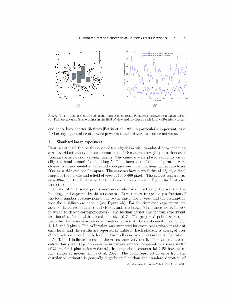
Fig. 3. (a) The field of view of each of the simulated cameras. Focal lengths have been exaggerated.(b) The percentage of scene points in the field of view and nucleus at each local calibration cluster.

and hence have shorter lifetimes [Estrin et al. 1999], a particularly important issuefor battery-operated or otherwise power-constrained wireless sensor networks.

4.1 Simulated image experiment

First, we studied the performance of the algorithm with simulated data modelinga real-world situation. The scene consisted of 40 cameras surveying four simulated(opaque) structures of varying heights. The cameras were placed randomly on anelliptical band around the “buildings”. The dimensions of the configuration werechosen to closely model a real-world configuration. The buildings had square bases20m on a side and are 2m apart. The cameras have a pixel size of 12µm, a focallength of 1000 pixels and a field of view of 600×600 pixels. The nearest camera wasat ≈ 88m and the farthest at ≈ 110m from the scene center. Figure 3a illustratesthe setup.

A total of 4000 scene points were uniformly distributed along the walls of thebuildings and captured by the 40 cameras. Each camera images only a fraction ofthe total number of scene points due to the finite field of view and the assumptionthat the buildings are opaque (see Figure 3b). For the simulated experiment, weassume the correspondences and vision graph are known (since there are no imagesin which to detect correspondences). The median cluster size for this experimentwas found to be 4, with a maximum size of 7. The projected points were thenperturbed by zero-mean Gaussian random noise with standard deviations of 0, 0.5,1, 1.5, and 2 pixels. The calibration was estimated for seven realizations of noise ateach level, and the results are reported in Table I. Each statistic is averaged overall realizations at each noise level and over all cameras/points in the configuration.

As Table I indicates, most of the errors were very small. The cameras are lo-calized fairly well (e.g. 45 cm error in camera centers compared to a scene widthof 220m, for 1 pixel noise variance). In comparison, commercial GPS have accu-racy ranges in meters [Bajaj et al. 2002]. The point reprojection error from thedistributed estimate is generally slightly smaller than the standard deviation of



Table I. Summary of the calibration errors for the simulated experiment, measured using themetrics in (4)-(8). The width of the scene in the experiment was 220m.

Noise Cerr Xerr uerr Mahal. cputimeσ

Method(cm)

Rerr ferr (cm) (pix) err (min)

Distributed 24.2 0.056 0.0025 21.9 0.39 0.79 300.5

Centralized 20.8 0.039 0.0020 15.0 0.46 0.96 427

Distributed 45.3 0.075 0.0052 23.3 0.76 0.76 541

Centralized 43.9 0.100 0.0031 20.2 0.83 0.83 433

Distributed 82.6 0.10 0.0091 25.8 1.15 0.77 831.5

Centralized 75.1 0.12 0.0059 27.2 1.14 0.81 449

Distributed 120.1 0.12 0.012 37.9 1.53 0.76 1862

Centralized 117.9 0.14 0.010 41.9 1.11 0.80 443

the noise (i.e. the Mahalanobis error is less than 1), as desired, and this relativemeasure of performance is roughly constant as the noise increases.

We also compared the distributed algorithm against centralized bundle adjust-ment, to determine if central bundling can create a substantial improvement. Toinitialize the centralized estimate, we registered all the cameras’ structure to acommon frame, averaged the multiple estimates of each scene point, and chosethe camera estimate that gave the lowest reprojection error. Importantly, Table Idemonstrates that the average accuracy of the distributed algorithm is about thesame as centralized bundle adjustment; for example, the error in camera centerlocalization for the distributed case is at most 8cm more than the error in thecentralized case (compared to an overall scene width of 220m). However, the dis-tributed estimate is computed much more quickly than the centralized estimate,as evidenced by the last column in Table I, which compares the average Matlabcputime required for each method and noise level (note that the centralized tim-ings do not include the time required to obtain the initial estimate). While thecentralized bundle adjustment takes roughly the same amount of time, regardlessof the noise level, the distributed algorithm is faster at lower noise levels. Whilethe distributed timings represent the total cputime required to estimate the struc-ture and camera parameters at all nodes, in practice, these computations wouldbe executed in parallel by all nodes independently, so the actual time required forcalibration would be substantially less than what Table I suggests. A major reasonfor the speed difference between the distributed and centralized algorithms is thatthe centralized bundle adjustment problem is an optimization over approximately9000 parameters, whereas each local bundle adjustment problem in the distributedscheme has an average of 1589 parameters (2423 in the worst case).

Figures 4a and 4b show the ground-truth configuration and the recovered con-figuration, respectively, for one noise realization with 1 pixel noise variance. Thequality of the shape recovery is evident. We emphasize that the only data used toobtain this result were the positions of matching points in the images taken by thecameras.

Figure 5a illustrates the communication graph for the simulated experiment, withan antenna range of 37m (the lowest range for which the communication graph isconnected). Figure 5b illustrates the vision graph. While there are many edgesACM Journal Name, Vol. 0, No. 0, 05 2006.


(a) (b)

Fig. 4. (a) Ground truth structure and camera positions for the simulated experiment. (b)Recovered structure and camera positions for a noise perturbation of 1 pixel. Focal lengths havebeen exaggerated.

1

2

3

4

5 6

7 8

91011121314

1516

17

18

19

20

21

22

23

24

2526

2728

29 30 31 32 3334

3536

37

38

39

40

(a)

1

2

3

4

5 6

7 8

91011121314

1516

17

18

19

20

21

22

23

24

2526

2728

29 30 31 32 3334

3536

37

38

39

40

(b)

Fig. 5. (a) Communication graph and (b) vision graph for the simulated experiment. The picturedcommunication graph was generated using an antenna range of 37m (the minimally connectedcase).

shared between the two graphs, there are also many edges in the vision graphthat require multiple hops to accomplish in the communication graph. Figure 6shows the number of messages handled at each node for the centralized (Figure6a) and distributed (Figure 6b) calibration algorithms, for the same antenna rangevalue of 37m. The total number of messages handled is comparable in both cases(766 for centralized vs. 748 for distributed). However, there is a relatively fairerutilization of the nodes in the distributed algorithm compared to the centralizedalgorithm (i.e. the centralized message distribution has a heavier tail). Nodes thatare frequently used will have lower lifetime due to the power consumed in sendingand receiving messages; the failure of such nodes would be catastrophic for thecentralized algorithm. On the other hand, failure of a node in the distributed caseis relatively less costly, since the calibration is maintained in a distributed stateacross the network.



0 10 20 30 40 50 600

2

4

6

8

10

12

14

16

Number of messages

Nod

e fr

eque

ncy

Total number of messages =766

(a)

0 10 20 30 40 50 600

2

4

6

8

10

12

14

16

Number of messages

Nod

e fr

eque

ncy


(b)

Fig. 6. Histogram of messages per node in the communication graph. (a) centralized calibrationvs. (b) distributed calibration in the simulated experiment, for an antenna range of 37m. Thecost for sending and receiving messages is assumed to be the same. The centralized messagedistribution has a much heavier tail than the distributed case.

40 60 80 100 120 140 160 180 200 2200

10

20

30

40

50

60

70

80

90

100

Antenna Range

Max

imum

mes

sage

s pe

r no

de

Centralized schemeDistributed scheme

Fig. 7. Maximum number of messages handled per node as a function of increasing antenna range,in the centralized (dashed line) and distributed (solid line) cases in the simulated example. Thedistributed algorithm always required a smaller worst-case number of messages per node.

Figure 7 shows the maximum number of messages handled by any node in thenetwork during the calibration algorithms as a function of increasing antenna range.In both cases, increasing the range makes the communication graph more connected.A more connected network generally places higher communication requirements onthe sink node for the centralized case.1 However, the maximum usage of any node

1Increasing the antenna range also increases the power required to send the messages, which wedo not model here.



1 2 3 4 5

6 7 8 9 10

11 12 13 14 15

A AD B BCE BCDE

ACD ACD B EFH EFHJ

G GHIJ FGHI IJ IJ

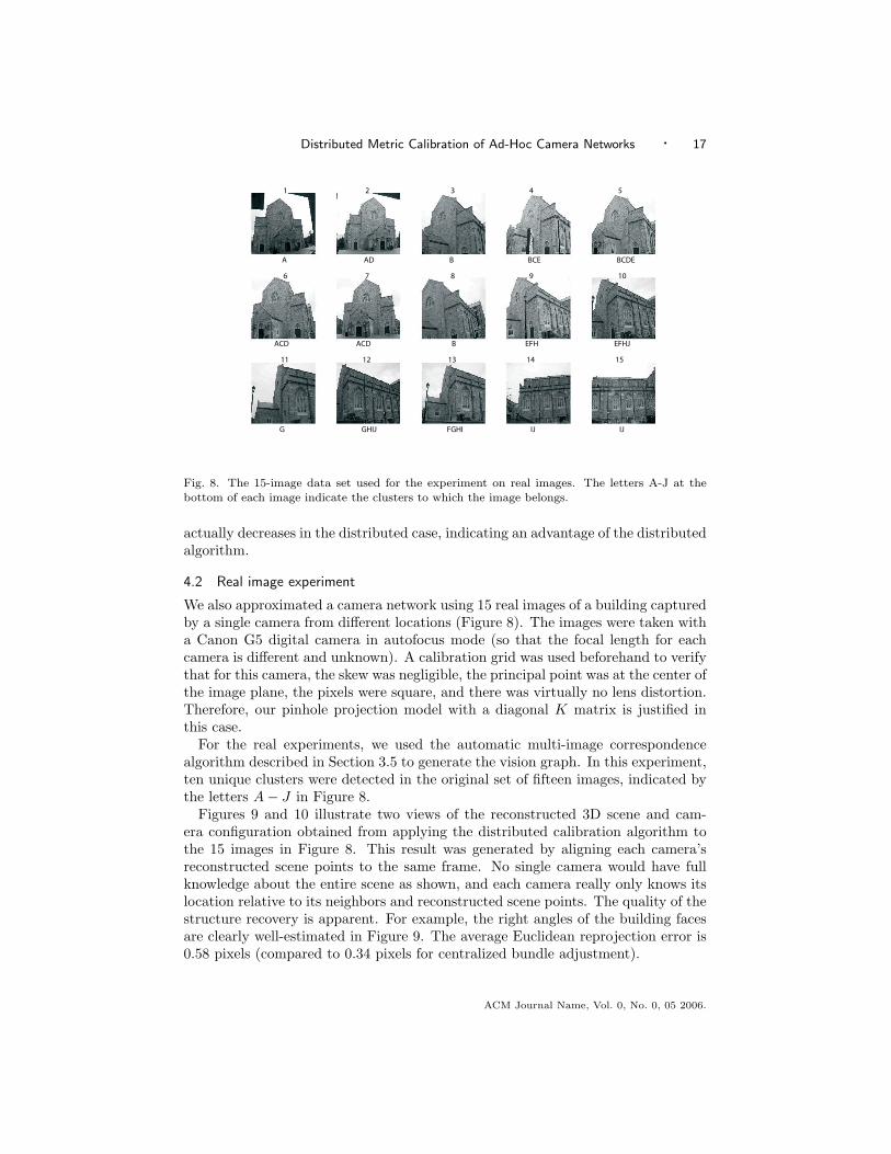
Fig. 8. The 15-image data set used for the experiment on real images. The letters A-J at thebottom of each image indicate the clusters to which the image belongs.

actually decreases in the distributed case, indicating an advantage of the distributedalgorithm.

4.2 Real image experiment

We also approximated a camera network using 15 real images of a building capturedby a single camera from different locations (Figure 8). The images were taken witha Canon G5 digital camera in autofocus mode (so that the focal length for eachcamera is different and unknown). A calibration grid was used beforehand to verifythat for this camera, the skew was negligible, the principal point was at the center ofthe image plane, the pixels were square, and there was virtually no lens distortion.Therefore, our pinhole projection model with a diagonal K matrix is justified inthis case.

For the real experiments, we used the automatic multi-image correspondencealgorithm described in Section 3.5 to generate the vision graph. In this experiment,ten unique clusters were detected in the original set of fifteen images, indicated bythe letters A− J in Figure 8.

Figures 9 and 10 illustrate two views of the reconstructed 3D scene and cam-era configuration obtained from applying the distributed calibration algorithm tothe 15 images in Figure 8. This result was generated by aligning each camera’sreconstructed scene points to the same frame. No single camera would have fullknowledge about the entire scene as shown, and each camera really only knows itslocation relative to its neighbors and reconstructed scene points. The quality of thestructure recovery is apparent. For example, the right angles of the building facesare clearly well-estimated in Figure 9. The average Euclidean reprojection error is0.58 pixels (compared to 0.34 pixels for centralized bundle adjustment).



Front wall

Entry way

Side wall

Roof lines

Fig. 9. Top view of the reconstructed 3D scene and camera configuration for the real experiment.The color of each scene point indicates to which of the clusters it belongs. The view illustratesthat points from different clusters are correctly aligned in the final scene. Arrows indicate featuresof the building that are recognizable in Figure 8.

Fig. 10. Another view of the reconstructed 3D scene and camera configuration for the real ex-periment. Reference lines are superimposed on the image for better perception. The viewpoint isroughly similar to image 9 in Figure 8.



1

2

3

4

5

6

7 8 9

10

11

12

13

14

15

(a)

1

2

3

4

5

6

7 8 9

10

11

12

13

14

15

(b)

Fig. 11. (a) Communication graph and (b) vision graph for the real experiment. The picturedcommunication graph was generated using a antenna range of 0.4 on a normalized scale in whichthe communication graph is first fully connected at range 1.0.

0 5 10 15 20 250

2

4

6

8

10

12

Number of messages

Nod

e fr

eque

ncy

Total number of messages = 62

(a)

0 1 2 3 4 5 6 7 8 90

2

4

6

8

10

12

Number of messages

Nod

e fr

eque

ncy


(b)

Fig. 12. Histogram of messages per node in the communication graph for the real experiment.(a) Centralized calibration, (b) distributed calibration. The communication graph was generatedusing a normalized range of 0.4. As in the simulated example, the distributed algorithm makesfairer use of the nodes.

As above, we computed and analyzed the number of messages handled by eachnode during both calibration algorithms. Since the ground truth camera locationsare unknown in this case, we built communication graphs for varying antenna rangesbased on the estimated positions of the camera nodes obtained at the end of thecalibration. The corresponding communication and vision graphs are shown inFigure 11. Figure 12 shows the node usage for the centralized and distributedcases. In the centralized case, the sink node is very heavily used while the rest ofthe nodes are used sparingly. The distributed scheme requires all the nodes to bearan approximately equal amount of communication load. Just as in the simulatedexperiment, the maximum number of messages handled by any node is much lessfor the distributed algorithm (a constant value of 9) than for the centralized one(between 25 and 27 depending on the antenna range).



5. CONCLUSIONS

We presented a distributed algorithm for the automatic, external, metric calibra-tion of an ad-hoc network of cameras with no centralized processor. Each cameraperforms a local, robust bundle adjustment over the camera parameters and scenepoints of its vision graph neighbors, starting from an initial point obtained by pro-jective factorization. We illustrated the accurate performance of the calibrationalgorithm using examples that modeled real-world camera networks, and showedthat the distributed algorithm results in a fairer allocation of messages per nodewhile achieving comparable accuracy to centralized bundle adjustment. There isstill much room for future work at this intersection of computer vision and sensornetwork research.

It is likely that real ad-hoc camera networks (e.g. cameras that are randomly de-ployed over a battlefield) might have a non-negligible fraction of nodes that cannotbe calibrated due to too little visual overlap with other nodes. In this case, time-of-flight or GPS-based localization schemes could be incorporated to get at leastcoarse estimates of such nodes’ positions. Also, the smaller a local cluster in thevision graph, the higher the possibility of entering a “critical” (i.e. mathematicallyunviable) configuration for the calibration problem. One could study how the localcluster formation process could be adjusted for the purposes of avoiding criticalconfigurations.

As discussed in Section 3.2, at the end of the calibration process described above,each camera has an estimate of its location and orientation relative to its neigh-bors. However, without additional processing, each of camera i’s neighbors mayhave a slightly different estimate of where i is, which may adversely affect visiontasks that require very high precision. Currently, we would deal with inconsis-tent estimates and achieve consensus in such cases simply by averaging multipleestimates when they occur (e.g., camera i’s final estimate of its location would be

1|i,Ci|

∑j∈i,Ci Cj

i , after the estimates have been registered by a similarity trans-formation). However, this is only the statistically “correct” answer when all theestimated parameters have the same covariance. Since this is never true in practice,we are developing more principled information fusion methods based on the under-lying probability densities of the estimated structure-from-motion parameters. Thedistributed framework makes it easy to incorporate graphical message-passing mod-els in order to achieve global consistency [Murphy et al. 1999]. The use of graphicalmodels for similar purposes has been recently investigated in the context of roboticsimultaneous location and mapping (SLAM), e.g. [Dellaert et al. 2005; Paskin andGuestrin 2004]. We note that while we expect methods based on graphical modelsto achieve better consensus, there may be tradeoffs with higher messaging overhead.Furthermore, the experiments in this paper indicate the agreement between nodescan already be quite good without enforcing global consensus.

To demonstrate the viability of the proposed distributed calibration scheme, theemphasis of this paper is on computer vision, and we have assumed idealized net-working conditions. We plan to build more realistic network models that modelthe power required to send or receive a message of a given length, and investigatenode lifetimes under realistic assumptions. We could further study the effects ofunequal or time-varying antenna ranges or channel conditions and dynamic net-ACM Journal Name, Vol. 0, No. 0, 05 2006.


work topologies. Since a realistic camera network is always changing, we couldmodel calibration as a continuous, efficient background process on the network toensure accurate performance on vision tasks. The graphical-model based approachwe are investigating will naturally handle the case of moving cameras. Eventually,we plan to build wireless camera nodes to test the performance of our algorithmsin real situations. We will adopt more advanced camera models (e.g. including lensdistortion) as the situation warrants.

Finally, we note that distributed camera calibration is only the first step towardsadditional distributed computer vision algorithms, such as handoff or cooperativetracking, view synthesis or image-based query and routing.

ACKNOWLEDGMENTS

Thanks to Dr. A. Abouzeid for valuable comments about the message-based analy-sis. Also, thanks to Dr. M. Pollefeys for providing projective-to-metric factorizationcode.

REFERENCES

Akyildiz, I., Su, W., Sankarasubramaniam, Y., and Cayirci, E. 2002. Wireless sensor net-works: a survey. Computer Networks 38, 393–422.

Andersson, M. and Betsis, D. 1995. Point reconstruction from noisy images. Journal of Math-ematical Imaging and Vision 5, 77–90.

Antone, M. and Teller, S. 2002. Scalable, extrinsic calibration of omni-directional imagenetworks. International Journal of Computer Vision 49, 2/3 (September/October), 143–174.

Avidan, S., Moses, Y., and Moses, Y. 2004. Probabilistic multi-view correspondence in adistributed setting with no central server. In Proceedings of the 8th European Conferenceon Computer Vision (ECCV). 428–441.

Bajaj, R., Ranaweera, S. L., and Agrawal, D. P. 2002. GPS: Location-tracking technology.IEEE Computer 35, 4 (April), 92–94.

Blazevic, L., Buttyan, L., Capkun, S., Giordano, S., Hubaux, J., and Boudec, J. L. 2001.Self-organization in mobile ad-hoc networks: the approach of terminodes. IEEE Communica-tions Magazine..

Capkun, S., Hamdi, M., and Hubaux, J. P. 2001. GPS-free positioning in mobile ad-hoc net-works. In Proceedings of the 34th Hawaii Iternational Conference On System Sciences (HICSS’01).

Choi, H., Baraniuk, R., and Mantzel, W. 2004. Distributed Camera Network Localization. InProceedings of the Asilomar Conference on Signals, Systems, and Computers. Pacific Grove,CA.

Chu, M., Haussecker, H., and Zhao, F. 2002. Scalable information-driven sensor queryingand routing for ad hoc heterogeneous sensor networks. Int’l J. High Performance ComputingApplications. Also Xerox Palo Alto Research Center Technical Report P2001-10113, May 2001.

Clarke, T. and Fryer, J. 1998. The development of camera calibration methods and models.Photogrammetric Record 16, 91 (April), 51–66.

Cormen, T. H., Leiserson, C. E., Rivest, R. L., and Stein, C. 2001. Introduction to Algorithms,2 ed. MIT Press.

Davis, L., Borovikov, E., Cutler, R., Harwood, D., and Horprasert, T. 1999. Multi-perspective analysis of human action. In Proceedings of the 3rd International Workshop onCooperative Distributed Vision. Kyoto, Japan.

Debevec, P. E., Borshukov, G., and Yu, Y. 1998. Efficient view-dependent image-based ren-dering with projective texture-mapping. In Proceedings of the 9th Eurographics RenderingWorkshop. Vienna, Austria.



Dellaert, F., Kipp, A., and Krauthausen, P. 2005. A multifrontal QR factorization approachto distributed inference applied to multirobot localization and mapping. In Proceedings ofNational Conference on Artificial Intelligence (AAAI 05). 1261–1266.

Devarajan, D. and Radke, R. J. 2004. Distributed metric calibration for large camera networks.In Proceedings of the 1st Workshop on Broadband Advanced Sensor Networks (BASENETS)2004 (in conjunction with BroadNets 2004). San Jose, CA.

Estrin, D. et al. 2001. Embedded, Everywhere: A Research Agenda for Networked Systems ofEmbedded Computers. National Academy Press. Washington, D.C.

Estrin, D., Govindan, R., Heidemann, J. S., and Kumar, S. 1999. Next century challenges:Scalable coordination in sensor networks. In Proceedings of ACM/IEEE Conference on MobileComputing and Networking (MobiCom 99). Seattle, WA, USA, 263–270.

Faugeras, O., Luong, Q.-T., and Papadopoulou, T. 2001. The Geometry of Multiple Images:The Laws That Govern The Formation of Images of A Scene and Some of Their Applications.MIT Press, Cambridge, MA, USA.

Fischler, M. A. and Bolles, R. C. 1981. Random sample consensus: A paradigm for modelfitting with applications to image analysis and automated cartography. Comm. of the ACM 24,381–395.

Fitzgibbon, A. W. and Zisserman, A. 1998. Automatic camera recovery for closed or openimage sequences. In Proceedings of the 5th European Conference on Computer Vision (ECCV’98). Springer-Verlag, London, UK, 311–326.

Garcia, M. A. and Solanas, A. 2004. Simultaneous localization and modeling from stereo vision.In Proceedings of the IEEE International Conference on Robotics and Automation (ICRA ’04).

Gortler, S., Grzeszczuk, R., Szeliski, R., and Cohen, M. 1996. The lumigraph. In Proceedingsof the Computer Graphics (SIGGRAPH ’96). 43–54.

Haas, Z. et al. 2002. Wireless ad hoc networks. In Encyclopedia of Telecommunications,J. Proakis, Ed. John Wiley.

Hartley, R. and Zisserman, A. 2000. Multiple View Geometry in Computer Vision. CambridgeUniversity Press.

Heyden, A. and Astrom, K. 1999. Flexible calibration: Minimal cases for auto-calibration. InProceedings of the 7th IEEE International Coference on Computer Vision (ICCV ’99). 350–355.

Horster, E., Lienhart, R., Kellermann, W., and Bouguet, J.-Y. 2005. Calibration of visualsensors and actuators in distributed computing platforms computing platforms. Tech. Rep.TR2005-11, University of Augsburg, Institute of Computer Science, University of Augsburg,Germany.

Kanade, T., Rander, P., and Narayanan, P. J. 1997. Virtualized reality: Constructing virtualworlds from real scenes. IEEE Multimedia 4, 1, 34–47.

Levoy, M. et al. 2000. The Digital Michelangelo Project: 3D scanning of large statues. InSIGGRAPH.

Lowe, D. G. 2004. Distinctive image features from scale-invariant keypoints. InternationalJournal of Computer Vision 60, 2, 91–110.

Mikolajczyk, K. and Schmid, C. 2003. A performance evaluation of local descriptors. InProceedings of the IEEE Conference on Computer Vision and Pattern Recognition. Madison,Wisconsin, 257–264.

Mikolajczyk, K. and Schmid, C. 2004. Scale and affine invariant interest point detectors.International Journal of Computer Vision 60, 1, 63–86.

Moezzi, S., Tai, L.-C., and Gerard, P. 1997. Virtual view generation for 3D digital video. IEEEMultimedia 4, 1 (Jan.-March), 18–26.

Murphy, K. P., Weiss, Y., and Jordan, M. I. 1999. Loopy belief propagation for approximateinference: An empirical study. In Proceedings of Uncertainty in Artificial Intelligence (UAI).467–475.

Niculescu, D. and Nath, B. 2003. Trajectory based forwarding and its applications. In Pro-ceedings of the ACM/IEEE Conference on Mobile Computing and Networking (Mobicom’03).ACM Press, New York, NY, USA, 260–272.



Obraczka, K., Manduchi, R., and Garcia-Luna-Aceves, J. 2002. Managing the informationflow in visual sensor networks. In Proceedings of the 5th International Symposium on WirelessPersonal Multimedia Communication (WMPC ’02).

Paskin, M. A. and Guestrin, C. E. 2004. Robust probabilistic inference in distributed systems.In Proceedings of the twentieth Conference on Uncertainty in Artificial Intelligence (UAI ’04).AUAI Press, Arlington, VA, USA, 436–445.

Pollefeys, M., Koch, R., and Van Gool, L. J. 1998. Self-calibration and metric reconstructionin spite of varying and unknown internal camera parameters. In Proceedings of the 6th IEEEInternational Conference on Computer Vision (ICCV ’98). 90–95.

Pollefeys, M., Verbiest, F., and Gool, L. J. V. 2002. Surviving dominant planes in un-calibrated structure and motion recovery. In Proceedings of the 7th European Conference onComputer Vision-Part II (ECCV ’02). Springer-Verlag, London, UK, 837–851.

Pottie, J. and Kaiser, W. 2000. Wireless integrated network sensors. Communications of theACM 3, 5 (May), 51–58.

Priyantha, N. B., Chakraborty, A., and Balakrishnan, H. 2000. The Cricket location-support system. In Proceedings of the 6th Annual ACM International Conference on MobileComputing and Networking (MOBICOM).

Rahimi, A., Dunagan, B., and Darrell, T. 2004. Simultaneous calibration and tracking witha network of non-overlapping sensors. In Proceedings of the IEEE Conference on ComputerVision and Pattern Recognition (CVPR 04). 187–194.

Schaffalitzky, F. and Zisserman, A. 2001. Viewpoint invariant texture matching and widebaseline stereo. In Proceedings of the 8th International Conference on Computer Vision (ICCV’01). Vancouver, Canada, 636–643.

Schaffalitzky, F. and Zisserman, A. 2002. Multi-view matching for unordered image sets, or“How do I organize my holiday snaps?”. In Proceedings of the 7th European Conference onComputer Vision (ECCV ’02). Vol. LNCS 2350. 414–431. Copenhagen, Denmark.

Seo, Y., Heyden, A., and Cipolla, R. 2001. A linear iterative method for auto-calibrationusing DAC equation. In Proceedings of IEEE Conference on Computer Vision and PatternRecognition (CVPR’01).

Sharp, G., Lee, S., and Wehe, D. 2002. Multiview registration of 3-D scenes by minimizingerror between coordinate frames. In Proceedings of the 7th European Conference on ComputerVision (ECCV ’02). Vol. LNCS 2351. 587–597. Copenhagen, Denmark.

Sinha, S. N., Pollefeys, M., and McMillan, L. 2004. Camera network calibration from dynamicsilhouettes. In Proceedings of IEEE Conference on Computer Vision and Pattern Recognition(CVPR)). 195–202.

Sturm, P. and Triggs, B. 1996. A factorization based algorithm for multi-image projectivestructure and motion. In Proceedings of the 4th European Conference on Computer Vision(ECCV ’96). 709–720.

Teller, S., Antone, M., Bodnar, Z., Bosse, M., Coorg, S., Jethwa, M., and Master, N.2001. Calibrated, registered images of an extended urban area. In Proceedings of the IEEEConference on Computer Vision and Pattern Recognition (CVPR ’01).

Triggs, B. 1996. Factorization methods for projective structure and motion. In Proceedings ofIEEE Conference on Computer Vision and Pattern Recognition (CVPR ’96). IEEE Comput.Soc. Press, San Francisco, CA, USA, 845–51.

Triggs, B., McLauchlan, P., Hartley, R., and Fitzgibbon, A. 2000. Bundle adjustment – Amodern synthesis. In Vision Algorithms: Theory and Practice, W. Triggs, A. Zisserman, andR. Szeliski, Eds. LNCS. Springer Verlag, 298–375.

Tsai, R. 1992. A versatile camera calibration technique for high-accuracy 3-D machine visionmetrology using off-the-shelf TV cameras and lenses. In Radiometry – (Physics-Based Vision),L. Wolff, S. Shafer, and G. Healey, Eds. Jones and Bartlett.

Umeyama, S. 1991. Least-squares estimation of transformation parameters between two pointpatterns. IEEE Transactions on Pattern Analysis and Machine Intelligence 13, 4, 376–380.



Wu, H. and Abouzeid, A. 2004a. Energy efficient distributed JPEG2000 image compression inmultihop wireless networks. In Proceedings of 4th Workshop on Applications and Services inWireless Networks (August 8-11). Boston, Massachusetts, USA.

Wu, H. and Abouzeid, A. 2004b. Power aware image transmission in energy constrained wirelessnetworks. In Proceedings of The 9th IEEE Symposium on Computers and Communications(ISCC’2004) (June 28-July1). Alexandria, Egypt.

Zhang, Z., Deriche, R., Faugeras, O. D., and Luong, Q.-T. 1995. A robust technique formatching two uncalibrated images through the recovery of the unknown epipolar geometry.Artificial Intelligence 78, 1-2, 87–119.

Zhang, Z. and Shan, Y. 2001. Incremental motion estimation through local bundle adjustment.Technical report, MSR-TR-01-54.

Received February 2005; September 2005; accepted May 2006


distributed metric calibration of ad-hoc camera networksrjradke/papers/radketosn06.pdf ·...

Documents