Discussion PaPer series

IZA DP No. 10596

Elizabeth U. Cascio

Does Universal Preschool Hit the Target?Program Access and Preschool Impacts

februAry 2017

Any opinions expressed in this paper are those of the author(s) and not those of IZA. Research published in this series may include views on policy, but IZA takes no institutional policy positions. The IZA research network is committed to the IZA Guiding Principles of Research Integrity.The IZA Institute of Labor Economics is an independent economic research institute that conducts research in labor economics and offers evidence-based policy advice on labor market issues. Supported by the Deutsche Post Foundation, IZA runs the world’s largest network of economists, whose research aims to provide answers to the global labor market challenges of our time. Our key objective is to build bridges between academic research, policymakers and society.IZA Discussion Papers often represent preliminary work and are circulated to encourage discussion. Citation of such a paper should account for its provisional character. A revised version may be available directly from the author.

Schaumburg-Lippe-Straße 5–953113 Bonn, Germany

Phone: +49-228-3894-0Email: publications@iza.org www.iza.org

IZA – Institute of Labor Economics

Discussion PaPer series

IZA DP No. 10596

Does Universal Preschool Hit the Target?Program Access and Preschool Impacts

februAry 2017

Elizabeth U. CascioDartmouth College, NBER and IZA

AbstrAct

IZA DP No. 10596 februAry 2017

Does Universal Preschool Hit the Target?Program Access and Preschool Impacts*

Despite substantial interest in preschool as a means of narrowing the achievement gap,

little is known about how particular program attributes might influence the achievement

gains of disadvantaged preschoolers. This paper uses survey data on a recent cohort to

explore the mediating influence of one key program attribute – whether disadvantage itself

is a criterion for preschool admission. Taking advantage of age-eligibility rules to construct

an instrument for attendance, I find that universal state-funded prekindergarten (pre-K)

programs generate substantial positive effects on the reading scores of low-income 4 year

olds. State pre-K programs targeted toward disadvantaged children do not. Differences

in other pre- K program requirements and population demographics cannot explain the

larger positive impacts of universal programs. The alternatives to universal and targeted

state pre-K programs also do not significantly differ. Together, these findings suggest that

universal preschools offer a relatively high-quality learning experience for low-income

children not reflected in typical quality metrics.

JEL Classification: H75, I24, I28, J13, J24

Keywords: early education, preschool, targeted, universal, access, quality

Corresponding author:Elizabeth U. CascioDartmouth College6106 Rockefeller HallHanover, NH 03755

elizabeth.u.cascio@dartmouth.edu

* I thank seminar and lecture participants at the Institute for Fiscal Studies, McMaster University, Montana State University, and Franklin and Marshall College for their comments. I also thank Diane Whitmore Schanzenbach for conversations that helped to motivate this research and Taryn Dinkelman, Ethan G. Lewis, and Na’ama Shenhav for helpful conversations and comments since then. All errors are my own.

I. Introduction

Over the past several decades, a consensus has emerged that the United States spends too

little on preschool education. This view is supported by considerable experimental and quasi-

experimental research pointing to large long-term social returns to preschool investments in

disadvantaged children – returns manifested in adulthood as increases in earnings and

educational attainment and reductions in violent crime and receipt of public assistance.1 Yet,

considerably less is known about the determinants of productive efficiency in preschool

education – how to make the dollars spent on preschool more beneficial.

The great diversity in state pre-kindergarten (pre-K) programs may reflect the relative

lack of research on the benefits associated with particular program characteristics. In 2014-15 –

the most recent school year with data available – not all states funded pre-K, and among the 42

states that did, there was great variation in how funds were allocated (Barnett et al., 2016). Some

state programs, like Florida’s, serve all 4 year olds that meet age-eligibility requirements

(“universal” programs) but otherwise have low standards; others, like Tennessee’s, are means-

tested or targeted on other risk factors (“targeted” programs), with stringent state requirements.

Yet other states – most famously, Georgia and Oklahoma – operate high-standard, universal

programs that have served as models for recent federal proposals to invest in early education.

In this paper, I take advantage of age-eligibility rules to estimate the short-term cognitive

and socio-emotional benefits of pre-K attendance in survey data where the mediating influences

of program characteristics can be directly assessed. My specific focus is on access – on the

impacts of using disadvantage as a criterion for admission. Universal pre-K programs may

deliver higher benefits than targeted pre-K programs for low-income children. For one, by being

                                                            1 For recent reviews of this literature, see Almond and Currie (2011), Elango et al. (2016), and Almond, Currie, and Duque (2017).

1

open to all, universal programs reach low-income children who do not meet the means tests of

targeted programs but would otherwise lack a preschool experience. In 2014, for instance, only

66.3% of 4 year olds were enrolled in any preprimary program (Snyder, de Brey, and Dillow,

2016), suggesting considerable scope to increase preschool attendance. Universal programs may

also be higher quality given observed inputs or program standards. They may attract better

teachers, set higher expectations, or be under more parental pressure to perform.

To my knowledge, no study to date has evaluated the efficacy of universal and targeted

programs for low-income children on the same basis – using the same data and research design.

Indeed, there is a mature body of research on targeted preschool programs, most famously the

federal Head Start program (e.g., Currie and Thomas, 1995; Garces, Thomas, and Currie, 2002;

Ludwig and Miller, 2007; Deming, 2009; Puma et al., 2010; Aizer and Cunha, 2012; Carneiro

and Ginja, 2014; Bitler, Hoynes, and Domina, 2014; Kline and Walters, 2016) and the “model”

preschool interventions of the distant past (e.g., Heckman et al., 2010; Schweinhart et al., 2005).2

There is also emergent research on state-funded universal preschools, based largely but not

entirely on the long-operating programs in Georgia and Oklahoma (e.g., Gormley and Gayer

(2005), Fitzpatrick (2008), Cascio and Schanzenbach (2013)). Data from the Birth Cohort of the

Early Childhood Longitudinal Study (ECLS-B) makes it possible to test formally whether

program access yields different short-term achievement effects for a recent cohort, born in 2001.

My analysis using the ECLS-B faces two challenges. The first is selection of children

into pre-K attendance. I address this challenge by taking advantage of the large differences in

pre-K attendance rates among preschool-aged children with birthdays near pre-K entrance cutoff

birthdates. While this source of variation is not new to the pre-K evaluation literature, the ECLS-

                                                            2 There are also several stand-alone studies of targeted state pre-K programs, for example in North Carolina (Ladd, Muschkin, and Dodge, 2014) and Tennessee (Lipsey et al., 2013).

2

B allows me to harness it in a new way.3 Instead of applying a regression discontinuity design

(RDD), I take a difference-in-differences (DD) approach, exploiting the relatively large

difference in pre-K attendance rates between 4 year olds in adjacent kindergarten cohorts in

states with robust state-funded pre-K programs. That is, I use a comparison group of other states

to remove the confounding effects of age and season of birth. This approach is more appropriate

than the RDD in this setting, where exact day of birth is not observed. More generally, survey

data allow me to overcome a number of limitations of previous RDD evaluations of pre-K, which

have relied on school administrative data (Lipsey et al., 2014). For example, by observing

outcomes for an entire cohort, I am in principle able to produce consistent estimates of the

impact of pre-K attendance using age eligibility as an instrument; rich background

characteristics, including pretests, also allow for new tests of internal validity.

The second challenge is that, just like the decision to operate a program at all, whether to

operate a universal or targeted program is arguably not random, but rather a function of a state’s

population, budget, and preferences. The overall standards of universal and targeted programs

nevertheless looked similar on average in the 2005-06 school year, when children born earlier in

2001 would have first been eligible to attend pre-K. For specific areas where there are

differences – indeed for all observed standards – I explore whether those differences mediate the

estimated effects in a regression framework. While variation in program standards is not random,

the approach is similar in spirit to that previously taken to understand variation in the impacts of

Head Start (Walters, 2015) and charter schools (Angrist, Pathak, and Walters, 2013; Dobbie and

Fryer, 2013). I also examine whether differences in demographics across universal and targeted

states, combined with heterogeneous treatment effects, can explain the findings.

                                                            3 Indeed, the literature has relied heavily on its use since Gormley and Gayer’s (2005) pioneering application of the RDD to Tulsa’s pre-K program. See, for example, Wong et al. (2008) and Weiland and Yoshikawa (2013).

3

I find substantial positive effects of attending universal pre-K on the cognitive test scores

of 4 year olds who qualify for free or reduced-price lunch (i.e., low-income children). By

comparison, low-income children do not benefit from pre-K targeted on income or other risk

factors. Universal pre-K attendance (eligibility) improves their early reading scores by a

statistically significant 1 (0.2) standard deviation; by contrast, the impacts of targeted pre-K

attendance on their early reading scores are statistically indistinguishable from zero and

significantly lower than those for universal pre-K attendance. A similar pattern of findings

emerges for the early math scores of low-income children, but the differences across universal

and targeted programs are not statistically significant.4 Though imprecise, achievement gains

from universal pre-K for higher-income children do not appear as large, suggesting that universal

pre-K diminishes early income achievement gaps.

The substantive findings hold up to a number of internal validity checks, and my

exploration of mechanisms suggests that variation in program access per se is their driving force.

Supporting a causal interpretation, the preferred specification does not predict developmental or

socio-emotional scores when children are toddlers, and substantive conclusions are little changed

after alterations to the control variables, the comparison group, and how the data are stratified.

Regarding mechanisms, both universal and targeted programs displace enrollment in other

center-based care for low-income children – and not differentially so – and differences in neither

state pre-K program standards nor state population demographics can explain the higher impacts

of universal programs for low-income children.

Taken together, these findings suggest that universal programs offer a relatively high-

quality learning experience for low-income 4 year olds not reflected in the quality metrics

frequently targeted by policymakers. To explore what this experience might look like, I conclude                                                             4 Findings for socio-emotional outcomes are unfortunately uninformative.

4

the paper with a descriptive analysis of pre-K teacher and school administrator interviews in the

ECLS-B. These data echo the differences in reported program standards, but also provide

insights into pre-K orientations and teacher attitudes. Targeted programs and universal programs

serving low-income children look similar along a lot of dimensions, but there is suggestive

evidence that they may have a stronger academic orientation. These findings are considerably

more speculative, however, and warrant exploration in future research, as does the importance of

direct peer effects in pre-K classrooms.

II. Program Landscape

There has been dramatic growth in public funding of preschool programs since the early

1980s. Figure 1 shows trends from 1968 through 2011 in the number of states funding preschool

(left axis) and in the Head Start and overall public preschool enrollment rates of 3 and 4 year

olds (right axis).5 In the early 1980s, only four states funded pre-K programs; by 2011, this

figure reached 40 states and the District of Columbia. Public preschool enrollment rates have

risen as more states have established pre-K programs. This is particularly the case for 4 year

olds, for whom enrollment in Head Start – the other primary provider of public preschool – has

been stagnant if not declining since the early 1990s. For 3 year olds, by contrast, public

preschool enrollment rates have risen alongside the funding expansions, but so too has Head

Start enrollment. This pattern reflects the focus of state-funded pre-K programs on 4 year olds.6

The time period relevant for the present study is the 2005-06 school year, represented by

the dashed vertical line in Figure 1. Thirty-eight states and the District of Columbia funded pre-K

                                                            5 Data on public preschool enrollment rates by age are calculated from the October Current Population Survey (CPS) School Enrollment supplements. Head Start enrollment rates divide Head Start enrollments reported by the Head Start Bureau by cohort size estimates based on Vital Statistics data on live births. State funding dates were constructed from program narratives published by NIEER (Barnett et al., 2016). 6 During the 2014-2015 school year, 29% of 4 year olds were enrolled in state-funded pre-K programs, compared to 5% of 3 year olds. These percentages have increased little since the 2009-2010 school year (Barnett et al., 2016).

5

programs at this time. In terms of access, some of these programs had no eligibility requirements

beyond those establishing the age of prospective enrollees – universal programs – whereas others

were means-tested or used risk factors other than poverty to determine eligibility – targeted

programs.7 Due to constraints imposed by my empirical approach, my analysis will focus on

state programs that served 4 year olds nearly exclusively, for which there were state-established

dates by which the youngest enrollees were to have been 4 years old, and for which those “cutoff

birthdates” did not fall in the middle of a month, according to statistics and program narratives

published by the National Institute for Early Education Research (NIEER) (Barnett et al., 2006,

2007).8 Sixteen states met these criteria for 2005-06, but I eliminate two from consideration due

to large divergence between NIEER-reported and ECLS-B-based enrollment figures.9

Though weighted toward states with larger programs due to these criteria, the remaining

14 states span the range of observed pre-K standards that existed in 2005-06. Figure 2 gives a

scatterplot of NIEER’s 10-point index of state program standards against its estimate of the

fraction of 4 year olds enrolled in the state-funded pre-K program.10 The dot sizes represent

Census estimates of the state’s 4-year-old population, and for comparison, I designate the 14

states of interest with their state postal codes. The (population-weighted) state-funded pre-K

                                                            7 Such risk factors include (but are not limited to) low parental education, single parenthood, English language learner (ELL) status, homelessness, placement in foster care, and development delays. 8 Specifically, I define “state programs that served 4 year olds nearly exclusively” as those for which the difference in NIEER-reported state pre-K enrollment rates for 4 year olds and 3 year olds was at least 8 percentage points. Twenty-two of the 38 states with state-funded programs in 2005-06 meet this criterion, Illinois being the last. Four of these 22 states (Vermont, Kentucky, Connecticut, and New Jersey) must be excluded due to local determination of their pre-K entry cutoff dates; two (Maine and North Carolina) must be excluded for having cutoff birthdates in the middle of the month. Of the remaining states with (smaller) state-funded pre-K programs, eight have age eligibility requirements that are locally determined. 9 These states are Louisiana and Michigan. Unfortunately, Barnett et al. (2006) does not report on Washington, D.C., so I cannot include ECLS-B observations from D.C. in the analysis. 10 One point on the index comes from comprehensive early learning standards; four come from teacher training and credentialing requirements (teacher has BA, specialized training in pre-K, assistant teacher has Child Development Associate (CDA) or equivalent, at least 15 hours of in-service training annually); two come from staffing ratios (maximum class size no larger than 20, staff-child ratio 1:10 or better); two come from comprehensive services (vision, hearing, health, and one support service, at least one meal provided); and one comes from a site visit requirement.

6

enrollment rate for 4 year olds for these 14 states was 34.5 percent in 2005-06, compared to only

10.3 percent for the remaining 24 states with programs.11 Most notably, of the five states with the

largest pre-K programs in terms of enrollment shares – Florida, Georgia, Oklahoma, Texas, and

Vermont – only Vermont is excluded from the analysis. Yet, states with lower enrollment rates

do appear in the analysis sample, and the distribution of the program standards index appears

similar across states with higher and lower enrollment rates.

Table 1 provides more detail on the programs in operation in 2005-06 in the 14 states of

interest, with states listed in descending order by 4-year-old enrollment rates and by whether the

program is universal (Panel A) or targeted (Panel B). The highest-access programs are the ones

in Georgia and Oklahoma, which as noted are the two longest-standing and most-studied

universal pre-K programs (Gormley and Gayer, 2005; Wong et al., 2008; Fitzpatrick, 2008,

2010; Cascio and Schanzenbach, 2013). The targeted programs include Tennessee’s, the only

state-funded pre-K program to date subjected to randomized evaluation (Lipsey et al., 2013). Ten

of the 14 states of interest require entering pre-kindergartners to be age 4 on August 31 or

September 1 – roughly the start of the typical school year – whereas three of the remaining four

states require pre-kindergartners to be age 4 one month later (September 30 or October 1).

The goal of this paper is to use the variation in age eligibility for pre-K associated with

these pre-K cutoff birthdates to estimate the effects of pre-K enrollment on age 4 cognitive and

socio-emotional test scores, and in particular to explore how those effects differ for low-income

children across universal and targeted programs. For the universal-targeted comparison to

cleanly reveal the additional benefits of universal access, it would ideally be the case that the two

types of programs on average had similar standards in 2005-06. Column 3 shows a small (and

                                                            11 In the analysis states, the population-weighted average (standard deviation) of the NIEER index is 5.94 (2.06). In the remaining states, these figures are 5.86 (2.11).

7

inconsistently signed) difference between the population- and enrollment-weighted values of the

10-point index for universal and targeted states, suggesting that this might be the case overall.

However, the remaining columns of the table show some differences for specific components of

the index. Most notably, targeted programs on average impose more teacher training and

credentialing requirements than universal ones, but are on average less likely to require small

classes and low staffing ratios. The difference in estimated effects between universal and

targeted programs is therefore at risk of picking up these differences in standards if they

independently affect the impacts of pre-K attendance. To address this possibility, I estimate

heterogeneity in the effects of pre-K by both access and state standards in some specifications.

III. Research Design

A. Intuition and Empirical Model

The basic relationship of interest is between state-funded pre-K attendance and children’s

academic and socio-emotional outcomes at preschool age. The fundamental identification

problem is that children who attend state-funded pre-K may have unobserved characteristics that

influence these outcomes directly. In targeted and universal programs alike, attendance is not

mandatory and programs themselves are often not fully-funded, allowing for potential selection

into enrollment based on unobserved characteristics. Simply controlling for observables in a

regression framework or pursuing other selection-on-observables methods, such as inverse

propensity-score weighting, are thus unlikely to uncover the causal effects of pre-K enrollment.

The approach taken in this paper is similar in spirit – but not in implementation – to that

taken first in the pre-K evaluation literature by Gormley and Gayer (2005).12 At base, I wish to

compare children with 4th birthdays near pre-K eligibility cutoff birthdates, the idea being that

children with 4th birthdays right on or before the cutoff should have a much higher probability of                                                             12 There have been many subsequent applications, including Wong et al. (2008) and Weiland and Yoshikawa (2013).

8

being enrolled in pre-K the following school year despite being on average similar in all ways –

observed and unobserved – to the children with 4th birthdays right after. If it were thus possible

to compare the short-term outcomes of children born right on the cutoff date to those born the

day after (e.g., September 1 versus September 2) – if it were possible to compare the preschool-

age outcomes of the oldest child in one school (e.g., pre-K) entry cohort to the youngest child in

the next – one could then recover the causal effect of pre-K eligibility and attendance.

In practice, the available data are insufficient to make such a sharp comparison: some

datasets, including the ECLS-B, lack information on exact day of birth, and even when

information on exact birthday is available, there are generally too few observations on a daily

basis to generate informative estimates. As a result, it is necessary to widen the range of

birthdates under consideration. Doing so requires acknowledging, however, that children with

birthdays on opposite sides of the cutoff date no longer have the same potential on average. In

fact, even if these children have similar unobserved characteristics, they differ along an observed

dimension – age – that is strongly related to child development. The RDD solution is to assume

that age effects on test scores are smooth, or can be modeled with a polynomial function in age

that is continuous through the birthdate cutoff.

In the current application, information on exact day of birth is not available, but

information on month of birth is, as are data on children across the U.S., not just in specific states

or school districts. These data support an alternative approach – a comparison of 4 year olds in

adjacent school entry cohorts in states with the pre-K programs of interest, as identified in

Section II (the treatment states), versus other states (the comparison states). In the treatment

states, cutoff birthdates for pre-K in fall 2005 were the same as cutoff birthdates for kindergarten

in fall 2006, so the children in adjacent pre-K kindergarten entry cohorts are also in adjacent

9

kindergarten entry cohorts. The comparison group then consists of the 22 other states that had a

state-established kindergarten cutoff birthdate in fall 2006 that was not in the middle of the

month.13 Differences in preschool-age outcomes across adjacent kindergarten entry cohorts in the

comparison group are intended to capture what would have happened for children in the

treatment states in the absence of pre-K, due to aging or other factors.

This is a DD rather than an RD design. Ignoring for now the distinction between

universal and targeted programs, the basic model of interest is

(1) ississisis vtreateligtreateligy ,

where yis is an age 4 (“preschool-age”) outcome (e.g., test score) of child i in state s; treats is a

dummy equal to one if state s is a treatment state (Table 1); and eligis is a dummy equal to one if

child i is in the earlier (older) school entry cohort, set to enter kindergarten in fall 2006 rather

than fall 2007 (or pre-K in fall 2005 rather than fall 2006, if pre-K is offered). More specifically,

eligis = 1[ageki - ageks* ≥ 0], where ageki is child i’s age in months on September 1, 2006, and

ageks* is the required minimum age in months for kindergarten entry in state s on September 1,

2006.14 So intuitively, if all states had September 1 cutoff birthdates for kindergarten entry, eligis

would equal one for children born January through August 2001, and zero for children born

September through December 2001.

The coefficient of interest in model 1 is θ, which captures how much more (or less)

kindergarten entry cohort relates to the preschool-age outcomes of children in treatment states. I

                                                            13 That is, comparison states were defined using all of the same criteria used to define treatment states except for the requirement of having a state pre-K program that served 4 year olds nearly exclusively. The comparison states thus include states without pre-K programs and states whose pre-K programs did not serve 4 year olds nearly exclusively (see footnote 8). For the second group of states, it would likely be impossible for me to detect a first stage using this research design. All comparison states are listed in the notes to Table 2. 14 Lacking information on exact day of birth, I must include children who are actually eligible for kindergarten in fall 2006 (e.g., those turning 5 on September 1, 2006 in a state with a September 1 cutoff date) in the fall 2007 kindergarten cohort. Assuming that births are (close to) uniformly distributed across the month, this should lead to a small amount of attenuation bias in estimates of the eligibility impacts. Thus, it is to minimize attenuation bias that I exclude states with cutoff dates closer to the middle of the month.

10

have designed the study so that θ is positive and both educationally and statistically significant

for pre-K attendance (the first stage). If, in turn, pre-K attendance improves test scores, it should

then be the case that there are relatively large preschool-age test-score differences associated

with being in the older kindergarten cohort in the treatment states. For estimates of θ to be

unbiased estimates of the impacts of pre-K eligibility – of intent-to-treat (ITT) effects – it must

be the case that differences in unobserved determinants of test scores across kindergarten cohorts

do not systematically differ across the treatment and comparison states (the exclusion

restriction).

To increase the chances that this is the case, I focus on a DD model with less restrictive

effects of eligibility and state of residence:

(2) issm

mismsisis veligtreateligy

7

4

,

where the eligism

represent a series of dummies for age in months relative to the minimum age in

months for kindergarten entry, or eligism

= 1[ageki - ageks* = m], where -4 ≤ m ≤ 7 (replacing γ

eligis in model 1),15 and αs represents a vector of state fixed effects (replacing α treats in model

1). Below, I provide informal evidence in favor of model 2’s identifying assumption that

0,cov issis vtreatelig by showing that children in the earlier kindergarten entry cohort in

treatment states generally do not have systematically different observed characteristics.

B. Distinctions from Existing Literature

Model 2 differs from the RDD models generally estimated in the pre-K evaluation

literature in a number of important ways. The first difference is theoretical: compared to the

RDD, model 2 does not require that age effects be continuous and smooth in the absence of pre-

                                                            15 Reflecting the fact that September 1 is the modal cutoff date (Table 1), I restrict the sample to children born in the eight months before their state cutoff date (0 ≤ ageki - ageks

*≤ 7) or in the four months after (-4 ≤ ageki - ageks*≤ -1).

I assess the sensitivity of the estimates to the choice of sample window in Table 5.

11

K. The use of eligibility indicators allows for effects that are discontinuous – even at the

eligibility threshold – which is helpful since when measured discretely, age is perfectly collinear

with season of birth, and season of birth effects need not be smooth. It is also helpful because

there could be increases in preschool enrollment at kindergarten eligibility thresholds even in the

absence of state-funded pre-K if private programs used state regulations to ration preschool slots

(Gelbach, 2002; Fitzpatrick, 2010).

Second, as it is generally implemented in this literature, the RDD does not cleanly

identify either the impacts of pre-K eligibility (ITT effects) or the impacts of pre-K attendance

(treatment-on-treated, or TOT effects). As described by Lipsey et al. (2014), the typical pre-K

RDD application has employed samples of pre-K students in adjacent school entry cohorts,

rather than the school entry cohorts in their entirety, because of a lack of outcomes data on

children who do not attend pre-K. I overcome this missing-data problem by using survey data

with outcomes on all individuals in a birth cohort, and I attempt to produce valid TOT estimates

(i.e., for the population at large) by instrumenting for pre-K attendance (prekis) in the model:

(3) issm

mismisis eligpreky

7

4

,

with eligis x treats, using two-stage least squares (TSLS). I also estimate model 3 using ordinary

least squares (OLS), for comparison.

Model 2 and my estimation of it differ from the standard implementation of the RDD in

this literature in other important ways.16 Unlike previous studies, I have ample data on baseline

characteristics with which to evaluate the internal validity of the research design, including birth

weight and earlier (age 2) test scores. I also not only observe but, via the use of a comparison

                                                            16 See Lipsey et al. (2014) for a description of the full range of potential problems inherent in previous applications of the RDD for pre-K evaluation.

12

group, can also evaluate impacts of pre-K on enrollment in alternative care and education options

for the same cohort of children affected by pre-K. Furthermore, the test score outcomes,

described below, are designed to be age-appropriate and are measured before children attending

pre-K would have progressed to kindergarten.

Finally, the data allow me to compare effects across states with different program

characteristics. The closest previous work in this vein is Wong et al. (2008), who use the age-

eligibility RDD to estimate the short-term cognitive effects of pre-K attendance in 2004-05 in

five states – Michigan, New Jersey, Oklahoma, South Carolina, and West Virginia. These states

differ in program access and standards, but the authors neither perform a formal analysis of the

influence of particular program characteristics, nor do they present estimates by family socio-

economic status, as is done in the present study. The present study also incorporates data from

more states that are also more variable in terms of program standards, as described in Section II.

IV. Data

A. Sample

The distinct approach taken in this paper is made possible by detailed survey data. These

data come from the Birth Cohort sample of the Early Childhood Longitudinal Study (ECLS-B).

The ECLS-B is a longitudinal survey of a stratified random sample of children born in the United

States in 2001.17 ECLS-B respondents were assessed and their parents and caregivers

interviewed at roughly 9 months of age (wave 1), 2 years of age/toddler age (wave 2), 4 years of

age/preschool age (wave 3), and kindergarten age (waves 4 and 5). My estimation sample

consists of all children with non-missing preschool-age cognitive assessments and demographic

and background characteristics residing at preschool age in one of the 14 treatment or 22

                                                            17 The ECLS-B contains oversamples of some demographic groups (Chinese and other Asians, Pacific Islanders, Native Americans, and Alaskan Natives), twins, and low and very low birth weight children. I apply sampling weights to make the estimates population representative.

13

comparison states and 5 years old between 8 months before and 4 months after their state’s

kindergarten entry cutoff – a total of 5,500 observations.18,19 Reported sample sizes are rounded

to the nearest 50, per IES rules to protect confidentiality of ECLS-B respondents.

Most pertinent for this study are the data from wave 3; this wave includes test scores on

children who were of preschool age, but may or may not have been actually enrolled in (or

eligible to enroll in) state-funded pre-K. More specifically, given the fall kindergarten entry

cutoffs in Table 1, the 2001 birth cohort can be split into two school entry cohorts in the wave 3

data – children eligible to enter kindergarten in fall 2006 (and pre-K in fall 2005, if relevant) and

children eligible to enter kindergarten in fall 2007 (and pre-K in fall 2006, if relevant). Children

were then tested starting in August 2005 – when any exposure to pre-K would have been limited

– through June 2006 – when a child enrolled would have had a full school year of exposure. The

average exposure to pre-K in treated states was 2.3 months, assuming September 1 starts the

school year.

B. Key Variables

The main outcomes of interest are cognitive test scores in early math and reading, as well

as socio-emotional test scores. The preschool cognitive assessment was designed to test both for

developmental (age-based) milestones and for knowledge and skills considered important for

school readiness and early school success.20 I work with reading and math scale scores from this

assessment normalized to mean zero and variance one in the full sample. The ECLS-B’s socio-

                                                            18 Restricting attention to respondents with non-missing cognitive assessments at wave 3 and non-missing demographic and family background information leads to a small number of drops from the full sample. The missing data are not predicted by the instrument. 19 Note that since the same comparison group is used to estimate the impact of targeted and universal programs, the number of observations may appear to be larger when summing across regression-specific sample sizes. 20 The preschool-age assessment drew on the Peabody Picture Vocabulary Test (PPVT), the Preschool Comprehensive Test of Phonological and Print Processing (Pre-CTOPPP), the PreLAS® 2000, and the Test of Early Mathematics Ability-3 (TEMA-3), as well as the cognitive assessment given to the fall 1998 kindergarten cohort of the ECLS (ECLS-K).

14

emotional assessment is based on coding of videotaped parent-child interactions in the “Two

Bags Task,” where a parent is asked to guide her child’s play with the contents of two bags – one

containing a book and the other some toys – over a ten-minute period. At preschool age, child

behavior on the task was assessed on three dimensions, each on a 7-point Likert scale –

engagement, quality of play, and negativity. I flipped the negativity scale (“positivity”), added

across the three scales, and standardized to mean zero and variance one in the full sample to

arrive at the socio-emotional test score used in this paper.

The ECLS-B also provides detailed information on the care and education of respondents

at preschool age. Following Bassok et al. (2016), I base my measures on provider reports of the

type of program in which a child was enrolled – pre-K, Head Start, other center-based care, or

informal non-parental care – where available, and parental reports where these data are missing;

the final category is parental care. Importantly, prek includes both public school and private

school programs; this is intentional, since many state-funded programs operate through private

schools or child care centers (Barnett et al., 2006). However, the ECLS-B does not directly

identify state-funded pre-K enrollment, and some centers or schools (or parents) might designate

a program as “pre-kindergarten” when it is not in fact the state-funded program. Thus, prek is a

misclassified measure of enrollment in the state-funded pre-K program. For this reason, the ITT

(model 2) estimates presented below are arguably more informative than the TOT ones (TSLS

estimates of model 3).21

The ECLS-B also contains rich family background information on respondents.22 In

addition to basic demographics (age at assessment and indicators for sex (female) and race (non-

Hispanic black and Hispanic)), I construct indicators for low-income (family income at or below

                                                            21 TSLS does not produce consistent estimates of coefficients on misclassified binary regressors (Bound, Brown, and Mathiowetz, 2001). 22 All time- or age-varying family background variables are measured in wave 3, or at preschool age.

15

185% of the federal poverty line (FPL)), for low birth weight (birth weight < 2,500 grams), for

low maternal education (at or below a high school degree), for a language other than English

being spoken in the home, and for the presence of both biological parents in the household. The

ECLS-B also assessed toddler’s motor and mental development and socio-emotional

development using the Bayley Short Form-Research Edition (based on the Bayley Scales of

Infant Development, 2nd Edition) and the Two Bags Task, respectively.23 I standardize these

measures analogously to the preschool-age outcomes.

I use the low-income indicator to stratify the analysis, and the remaining background and

demographic characteristics as baseline regression controls. The low-income indicator is ideal

for stratification, since free or reduced-price lunch eligibility (family income ≤ 185% FPL) is the

modal income eligibility criterion for the targeted states of interest.24 In specification checks, I

estimate the preferred model (with baseline regression controls) for the toddler-age “pretests,” as

well as include pretest scores as additional controls in the main test score model. If model 2

identifies the effect of age eligibility for pre-K, the inclusion of these variables as controls should

improve the precision of the estimates without greatly affecting their magnitudes.

C. Preliminary Evidence on Identifying Assumptions

Recall that the validity of my empirical approach rests on two assumptions. The first is

that eligis x treats predicts pre-K enrollment (first stage). The second is that eligis x treats does not

predict unobserved correlates of the outcomes of interest (exclusion restriction). The remainder

of this section provides some preliminary evidence on whether these assumptions are met.

                                                            23 In wave 2, the child behavior scores are for engagement, negativity, and sustained attention. 24 The eligibility criterion is relevant for four targeted states – Texas, Maryland, Colorado, and Tennessee – which together account for 61 (73) percent of 4-year old population (state-funded pre-K enrollment) in the states with targeted programs listed in Table 1. The remaining states have tighter income eligibility requirements (Kansas) or no explicit income requirements, but risk factor requirements that correlate strongly with income (Illinois, South Carolina, Virginia). I test the sensitivity of my conclusions to how the data are stratified in a specification check.

16

Figure 3 shows evidence on the first stage, focusing on low-income children.25 To

elucidate how the DD estimates more generally are constructed, Panel A shows raw means of

pre-K enrollment at preschool age (in 2005-06) by state of residence and by age relative to the

minimum age for kindergarten entry. I group state of residence into the three pertinent groups –

universal states, targeted states, and comparison states – and to reduce noise, I group the age

variable into two-month intervals. Age is increasing along the horizontal axis, with the first two

points representing ages at which children in treatment states would not have been eligible to

attend pre-K in fall 2005, i.e., children in the 2006 (2007) rather than 2005 (2006) pre-K

(kindergarten) entry cohort. Panel B then shows the difference in means between each treatment

group and the comparison group, relative to (or subtracting off) what that difference was for the

children who just missed eligibility (-2 ≤ ageki - ageks*≤ -1). Aside from age being grouped into

intervals, this is the generalized version of model 2, and thus matches the DD estimates.

As shown in Panel A, all three groups of states have fairly similar 2005-06 pre-K

enrollment rates among low-income children who were not eligible to attend pre-K

(kindergarten) until fall 2006 (2007). However, a substantial gap between the treatment and

comparison states emerges for children eligible to start pre-K (kindergarten) in fall 2005 (2006).

Panel B shows that the treatment-comparison gap in 2005-06 pre-K enrollment rates is between

10 and 25 percentage points larger among eligible children than among those who just missed

eligibility. Estimates are larger – and more likely to be statistically significant – for universal

states than for targeted ones. Consistent with Panel A, there is also some evidence of a treatment-

comparison difference in 2005-06 pre-K enrollment rates among younger children (those missing

pre-K eligibility by 3 or 4 months), but these differences are not statistically significant.

                                                            25 Analogous plots for children who are not low-income are shown in Figure A1. There is evidence for this population of a first-stage relationship for universal states but not for targeted states, as expected.

17

Table 2, Panel A shows the corresponding DD estimates of this first-stage relationship,

i.e., subgroup-specific coefficients (standard errors) on eligis x treats from model 2.26 Continuing

with the intuition from Figure 3, these are regression-adjusted differences-in-differences in 2005-

06 pre-K enrollment rates between the 2006 and 2007 kindergarten cohorts in the treatment

(universal or targeted) states versus the comparison states. To match the specifications later

estimated, the underlying regression models now include indicators for month of assessment in

addition to the eligism indicators and state of residence fixed effects.27

Consistent with the graphical evidence, the coefficient on eligis x treats is relatively large

for low-income children in universal states (column 2). This coefficient estimate is 0.207,

implying that the gap in 2005-06 pre-K enrollment rates for low-income children between the

2006 and 2007 kindergarten cohorts is 20.7 percentage points higher in states with universal pre-

K programs than in the comparison states. For low-income children in targeted states, this gap

amounts to 15.6 percentage points, and for higher-income children in states with universal

programs (column 4), this gap is similar, at 15.7 percentage points. In each case, the coefficient

estimate is statistically different from zero but arguably lower than might be expected, possibly

because the ECLS-B measure of pre-K enrollment is a misclassified measure of enrollment in

state-funded pre-K programs, as noted above.28,29 For higher-income children in targeted states

(column 8), the coefficient estimate is smaller and not significant.

                                                            26 As in Figure 3, I cluster standard errors on state of residence-by-month of birth (the level of the treatment) and weight the analysis using sampling weights. 27 Figures A7 and A8 show that the first-stage “event study” estimates look fairly similar with controls for month of assessment and for baseline background characteristics versus without. 28 In the absence of misclassification but with perfect compliance (i.e., all children starting pre-K only when they are age eligible), the first-stage DD coefficient would be the 2005-06 academic-year DD in pre-K enrollment rates between 3 and 4 year olds in treatment versus comparison states. Across all states with universal pre-K (Table 1, Panel A), the (population-weighted) difference in age 3 and age 4 enrollment rates is 41.2 percentage points; for states with targeted pre-K programs, this figure is 24.1 percentage points; and for the 22 comparison states, this figure is 4.2 percentage points. With perfect compliance, we might therefore expect to see first-stage estimates of 37 (41.2-4.2) percentage points for universal programs and 19.9 (24.1-4.2) percentage points for targeted programs.

18

Panel B then shows the analogous estimates for the baseline demographic and

background characteristics. As earlier described, these estimates provide an informal test of the

exclusion restriction; if model 2 is identified (or model 3 identified when estimated using TSLS),

eligis x treats should have little predictive power with regard to these observed correlates of test

scores. And indeed, these estimates suggest that age-eligibility rules provide for relatively clean

identifying variation for low-income children. For low-income children in both groups of

treatment states (columns 2 and 6), the coefficients are both individually and jointly statistically

insignificant. With the exception of having higher Hispanic shares and higher likelihoods of

speaking a language other than English, low-income children also look fairly similar to one

another across the two groups of states (columns 1 and 5). Higher-income children also look

better than low-income children on many observed dimensions (column 3), as expected.

However, the balance test fails more often for higher-income children in universal states.30

Overall, Table 2 suggests that comparisons of impacts of universal versus targeted pre-K

for low-income children should be fairly informative, but more caution may be in order when

making comparisons of impacts of universal pre-K across low- and higher-income children.

Further, even if not statistically significant, the sometimes large coefficient magnitudes in Table

2 suggest that estimates including background controls are preferable to those without.

V. Findings

A. Baseline Results

                                                                                                                                                                                                Perfect compliance is untenable, however; existing research on kindergarten entry (e.g., Cascio and Schanzenbach, 2016) suggests that non-compliance with age-eligibility rules is likely to reduce the gaps for universal programs by on average 20%, but by a greater extent for higher-income children. If, for example, there were a 30% non-compliance rate for higher-income children and a 10% one for low-income children, the first-stage DD coefficients would be 33.2 percentage points for low-income children in universal programs, 21.7 percentage points for low-income children in targeted programs, and 25.9 percentage points for higher-income children in universal programs, consistent with attenuation bias on the order of 30% to 40%. 29 Suggestive of misclassification is the high pre-K enrollment rate of higher-income children in targeted programs. 30 This seems an unfortunate consequence of sampling variation, since there is arguably little sorting around these cutoff dates (Dickert-Conlin and Elder, 2010).

19

Table 3 presents, separately for each of the four access-by-income subgroups and each of

the three test scores, least squares estimates of the effects of age-eligibility for pre-K from model

2 and both TSLS and OLS estimates of the effect of pre-K attendance from model 3. All of the

regressions include the eligibility indicators (the eligism), state fixed effects, month of assessment

dummies, and the demographic and background variables listed in Table 2, Panel B as controls.31

Mean test scores for the ineligible sample in treatment states (row 1 of each panel) show the

large gaps in test scores by SES that emerge even at an early age.

Against this backdrop, consider the estimates for preschool-age reading scores, shown in

Panel A. For low-income children in states with universal pre-K programs (column 1), the

estimated DD coefficient from model 2 is a statistically significant 0.229. This implies that the

gap in 2005-06 school year reading test scores between low-income children in the 2006 and

2007 kindergarten cohorts is about 0.23 standard deviations higher in states with universal pre-K

programs than in the comparison states. When this estimate is scaled by the corresponding first-

stage DD coefficient for prek – or when I instrument for prek in model 3 with eligis x treats using

TSLS – I predict that universal pre-K attendance brings about a 1.109 standard deviation

improvement in reading scores at preschool age. This figure is inflated over what would have

been achieved if prek were not a misclassified measure of state-funded pre-K attendance, but

even absent misclassification, the effect size would have been substantial.32 By comparison, the

OLS estimate of the pre-K attendance effect is much smaller and not statistically significant,

suggesting that conclusions are very different assuming only selection on observables.33

                                                            31 Estimates of these same models without the demographic and background controls are in Appendix Table A1. Throughout, standard errors are clustered on state-by-month of birth, and estimates weighted by sampling weights. 32 For example, the back-of-the-envelope prediction of the first-stage coefficient in the absence of misclassification (footnote 28) would be consistent with a TSLS impact of 0.69 standard deviation. 33 Magnuson, Ruhm, and Waldfogel (2007) also find evidence of much larger effects of pre-K attendance on cognitive test scores using TSLS over OLS in a study using data from the ECLS-K.

20

State-funded pre-K appears to be more effective for low-income children when programs

are universal rather than targeted. Column 3 shows that the gap in 2005-06 school year reading

test scores between low-income children in the 2006 and 2007 kindergarten cohorts was actually

more positive in the comparison states than in the targeted states; the DD estimate is negative.

Though statistically insignificant, this DD estimate is significantly different from the DD

estimate for low-income children in universal pre-K, in column 1. The same general pattern (but

not significance) of estimates emerges for math scores (Panel B), and though not individually

significant, estimated effects of pre-K eligibility on the socio-emotional scores of low-income

children are also marginally significantly higher for universal programs than for targeted ones

(Panel C).

Figure 4 shows graphical evidence of the impacts of pre-K attendance on reading scores

for low-income children like what was shown for their pre-K attendance in Figure 3. There is a

fairly strong age gradient in scores among all groups of states (Panel A). However, a relatively

large treatment-comparison test score gap among eligible children only emerges for universal

states (Panel B). Indeed, targeted and comparison states have very similar reading scores for low-

income children on average regardless of age, despite the significantly higher pre-K enrollment

rates among eligible children in targeted states (Figure 3, Panel B). Figures A2 and A3 provide

the analogous graphs for math and socio-emotional scores of low-income children.34 Graphical

evidence of impacts of universal pre-K here is weaker, consistent with the relative lack of

statistical significance of the findings for these outcomes.

Universal pre-K also appears to boost the academic performance of low-income children

more than higher-income children. The estimated effects of universal pre-K on the cognitive test

scores of higher-income children are close to zero and not statistically significant (column 2,                                                             34 Figure A7 provides event-study coefficients for all outcomes from a model with the same controls as in Table 3.

21

Panels A and B). On the other hand, I cannot reject equality of the effects of universal pre-K

(eligibility or attendance) across family income for any of the outcomes, and as earlier noted, the

column 2 estimates may be less credible, making me hesitant to draw strong conclusions. Yet,

such a finding would be consistent both with a framework where higher-income children have

relatively high-quality care and education options in the absence of universal pre-K and with

much existing evidence on universal preschools both in the U.S. and worldwide (Cascio, 2015;

Elango et al., 2016).35

To summarize, the baseline differences in the impacts of targeted and universal pre-K for

low-income children are statistically and economically meaningful. The small implied effects of

targeted state pre-K programs are consistent with findings from the Head Start Impact Study

(Puma et al., 2010; Kline and Walters, 2016) and from the experimental evaluation of the

(targeted) Tennessee Voluntary Pre-K program (Lipsey, et al., 2013), both of which focus on

similarly recent cohorts. In addition, the large implied effects of universal pre-K attendance on

cognitive test scores are in line with recent estimates of the effects of school exposure at young

ages.36 This pattern of findings suggests that universal pre-K programs are more like “school” in

their effects than targeted ones. The effect sizes also suggest that universal pre-K attendance can

(more than) close test score gaps by income that exist prior to pre-K entry; eligibility for pre-K

alone cuts reading test score gaps by income by nearly a third.

B. Robustness Checks

                                                            35 See Figures A4, A5, and A6 for graphs akin to Figure 4 for the reading scores, math scores, and socio-emotional scores of higher-income children. Figure A8 then provides event-study coefficients from a model with the same controls as in Table 3. 36 For example, taking advantage of variation in eligibility for school entry using the RDD in the ECLS-K, Anderson et al. (2011) estimate that children who have completed first grade have reading (math) test scores that are on average 1 (0.776) standard deviation higher than children of the same age who have only completed kindergarten. Relying on quasi-random variation in test dates in the ECLS-K, Fitzpatrick, Grissmer, and Hastedt (2011) also estimate that a year of kindergarten or first grade raises test scores by about one standard deviation.

22

For the estimates in Table 3 to identify the effects of pre-K, it must be the case that there

are no other reasons to believe outcomes would have differed with eligibility (or across

kindergarten entry cohorts) more in the treatment states than the comparison states. I have

already provided some evidence consistent with this assumption, namely the tests for balance on

observables in Table 2. In the remainder of this section, I provide further evidence and probe the

sensitivity of the estimates to additional controls, the choice of comparison group, and alternative

ways of stratifying the data.

One concern is that, though the interaction between treatment state and age eligibility for

pre-K may not be strongly associated with observables that predict performance (Table 2), it

could still be associated with unobservables: eligible children in treatment states might have

greater unobserved potential conditional on their observables. If so, we might expect to see an

“effect” of age eligibility for targeted pre-K on the test scores of higher-income children. But this

is not the case (Table 3, column 4). If it existed, such a correlation between the instrument and

unobservables would also arguably appear earlier in life, before children are preschool age.

Table 4 explores this possibility, presenting estimates of the same models in Table 3 but for

developmental and socio-emotional test scores at age 2. Regardless of the outcome variable, the

DD coefficients are relatively close to zero (often negative), statistically insignificant, and not

statistically different from one another. Relatedly, the second row of each panel of Table 5 shows

that, when age 2 scores are included as controls in the models for reading scores (Panel A) and

pre-K enrollment (Panel B), the DD estimates are similar to what they were at baseline.

The remainder of Table 5 shows the DD estimates for reading scores and pre-K

enrollment under other modifications to the specification.37 The first modification is to the

                                                            37 To conserve on space, the corresponding estimates for math and socio-emotional scores are in Appendix Table A2.

23

comparison group: instead of including all 22 states, I limit attention to the 13 comparison states

that have pre-K programs; by revealed preference, these states may be more similar to the

treatment states, and thus may do a better job of representing the counterfactual.38 This sample

restriction increases the estimated impacts of universal pre-K eligibility on the reading test scores

of low-income children without appreciably changing impacts on pre-K enrollment. Focusing on

a narrower window of observations around the cutoff dates also reinforces the conclusion that

universal pre-K programs outperform targeted ones for low-income children in terms of reading.

The next two rows consider different ways of stratifying the sample. Stratifying by low

maternal education again strengthens the conclusion that disadvantaged children benefit

relatively more in terms of reading scores from universal pre-K. On the other hand, stratification

by family income at or below 130% FPL (the cutoff for free lunch eligibility) somewhat weakens

the difference in pre-K eligibility effects on reading scores for low-income children in universal

and targeted states. To explore the relationship between family background and the effects more

non-parametrically, Figure 5 plots DD estimates of the impacts of pre-K eligibility on pre-K

attendance and reading scores by quintiles of a socio-economic status (SES) index derived from

factor analysis on parental education, parental occupation, and family income. Universal pre-K

eligibility yields statistically significant attendance effects through the fourth quintile of the

index, whereas first-stage estimates for targeted programs diminish monotonically in the index

(Panel A). The corresponding DD estimates for reading scores (Panel B) suggest that the benefits

of universal pre-K decline in SES. In general, these findings suggest that my baseline

stratification of the sample by free- or reduced-price lunch eligibility captured the key elements

of the effects in the data.

                                                            38 Recall that these 13 states are not treatment states either because their pre-K programs are too small or because those programs serve a high share of 3 year olds relative to 4 year olds, based on external (NIEER) data. In both cases, it would likely be difficult to detect a first stage impact on pre-K enrollment.

24

VI. An Effect of Program Access?

Thus far, I have shown that universal pre-K delivers larger short-term test score benefits

than targeted pre-K for disadvantaged children. The estimates for universal programs are

substantively similar to the short-term effects of universal kindergarten, while the estimates for

targeted programs are substantively similar to those for targeted early education (e.g., Head

Start) in recent cohorts. And while point estimates (and thus effect sizes) are somewhat sensitive

to specification, a larger impact of universal pre-K on disadvantaged children’s test scores –

reading scores in particular –has emerged across all of the robustness checks considered.

But does universal access per se cause universal programs to be more productive? Not

necessarily. Even if eligibility for pre-K is “as good as random” at the individual level, program

access at the state level may be related to other state-level factors that make pre-K attendance

more or less productive. For example, Table 1 showed that the universal pre-K programs of

interest in operation in 2005-06 were more likely than targeted ones to require class sizes at or

below 20 students and student to staff ratios of 10:1 or better (combined under the “Staffing”

column of Table 1). If lower class sizes increase program benefits, class size requirements might

be the actual explanation for the universal-targeted impact differential, or may diminish that

differential substantially.39 Likewise, if there is sufficient demographic heterogeneity in the

effects of pre-K, differences in the demographics of the low-income populations in targeted and

universal states (Table 2) could be contributing to the estimates. Further, the early childhood care

and education landscape might be different in states with universal pre-K programs.40 If there

                                                            39 Findings from Project STAR (Krueger, 1999; Chetty et al., 2011) suggest that assignment to a small class in kindergarten yields immediate cognitive test score benefits, particularly for disadvantaged children, though not as large as the effects of exposure to universal pre-K for low-income children estimated here. 40 The establishment of universal programs may in fact change the child care and early education sectors. See, for example, Bassok, Fitzpatrick, and Loeb (2014) and Bassok, Miller, and Galdo (2016).

25

were fewer center-based care alternatives to universal pre-K, for instance, I would expect to find

relatively large test score effects of universal pre-K, all else constant.41

Table 6 considers this last possibility, showing DD estimates of eligibility impacts from

model 2 for “counterfactual” care – Head Start, other center-based care, informal non-parental

care, and parental care. These variables are mutually exclusive and, along with pre-K, span the

space of possible education and care options for preschool-age children; the DD coefficients

therefore add up to zero across all categories. The DD coefficients for pre-K (Panel A) are the

first-stage coefficients on the instrument for the TSLS estimates presented in Tables 3 and 4.

With the exception of a marginally significant reduction in the likelihood of Head Start

enrollment among children in targeted programs (column 6), none of the DD estimates for the

alternative care options (Panel B) are statistically significant for low-income children (columns 2

and 6). While the implied effects of pre-K attendance on the Head Start enrollment of low-

income children are larger in magnitude for targeted than for universal programs, I cannot reject

equality of the DD coefficients for any of the variables, including pre-K attendance.42 Overall,

these findings provide at best weak evidence that cross-state differences in counterfactual care

options explain the relative efficacy of universal programs.

To address the first possibility, I then estimated the effect of pre-K eligibility holding

constant each of the NIEER program standards, one-by-one, using the model:43

(4) ispp p

ppisspm

pmismp

ssisQsisTssisUTisp

PxPelig

Qtreateligtreateligunitreateligy

1

0

1

0

7

4

,

                                                            41 In re-analyses of data from the Head Start Impact Study, Feller et al. (2015) and Kline and Walters (2016) find that Head Start has much smaller impacts on children who would have otherwise been in center-based care. 42 Likewise, I cannot reject equality of effects on overall (formal) preschool enrollment, which sums across pre-K, Head Start, and other formal centers. 43 Estimates are very unstable when attempting to include all 10 standards in a linear and additive way.

26

where p indexes the estimation sample, with p=1 for universal pre-K estimates and p=0 for

targeted pre-K estimates, and so Pj =1[j=p]. unis and treats represent, respectively, a dummy for

whether s is a universal (treated) state and a dummy for whether s is a universal or targeted

(treatment) state, and Qs a dummy set to one if a particular state pre-K program standard was met

in s in 2005-06. Because all of the regression controls are interacted with an indicator for the

estimation sample, in a version of the model excluding eligis x treats x Qs, the triple-difference

coefficient, θUT, generates the difference in the DD estimates for universal and targeted pre-K

programs presented in Table 3; the coefficient θT then reproduces the DD estimate for targeted

programs.

The interest here is then in the model as written, with eligis x treats x Qs included. This

model adjusts estimates of θUT for the correlation between program access and the program

standard in question, Qs. Analogous to the interpretation of θUT, the coefficient θQ gives the

difference in DD coefficients for state pre-K programs with versus without standard Qs. If this

coefficient is positive – if a program with standard Qs appears more productive – and if universal

programs are more likely to have standard Qs than targeted ones – estimates of θUT with eligis x

treats x Qs included will be lower than at baseline.

Table 7 presents estimates of θUT and θQ for each standard; for comparison, baseline

estimates, without the control for standards, are shown in column 1.44 The table focuses on

reading scores and pre-K attendance rates of low-income children; estimates for math and socio-

emotional scores for this subpopulation are in Appendix Table A3. The largest erosion in the

relative reading score benefits of universal programs comes from holding constant teacher BA

requirements (column 3), staffing/class size requirements (column 6), and the site visit

                                                            44 I pool the program standards for class size and staffing ratios into one dummy because there is such limited independent variation in these standards.

27

requirement (column 10). The final two cases are anticipated: universal programs are more likely

to have these standards, and these standards are associated with higher (though not statistically

significant) benefits from pre-K attendance. Even so, the universal-targeted difference in DD

coefficients remains sizable and statistically significant in both cases. And for the specification

including the interaction between eligibility and a teacher BA requirement, the estimate of θUT is

nearly statistically significant (p-value=0.124). In addition, the (insignificant) estimate of θQ in

this specification is negative, suggesting that low-income children in states where programs have

teacher BA requirements gain less from pre-K. While a null effect of teacher education

requirements might be expected given decades of related findings in the literature on K-12

education, a negative effect is not.45

A potential cause of this unexpected finding is that model 4 forces the same effect of each

program standard on both universal and targeted programs. An alternative way to think about the

relative importance of universal access and these standards is thus to ask how standards interact

with access. For example, do universal programs without teacher training and credentialing

requirements actually perform better than those with such requirements? If so, it would suggest

that we might want to take seriously the findings shown in Table 7, column 3. Similarly, do

targeted programs with class size requirements produce effects on reading scores as large as

those found for universal programs? If so, it might suggest that it is indeed class size rather than

access that is driving the relative efficacy of universal programs.

The scope for testing whether there are differences in the effects of standards by access is

unfortunately limited by the available policy variation. But there is still insight into these

questions to be had. In particular, among universal states, Florida lacks any teacher teaching or

                                                            45 This finding could reflect negative selection of states that require pre-K teachers to have BAs. That program standards are not randomly assigned is of course a key limitation of this exercise.

28

credentialing requirements but has both NIEER staffing requirements. On the flip side, among

states with targeted programs, Texas lacks the staffing requirements but mandates three of the

four NIEER teacher training and credentialing requirements, including the teacher BA

requirement (Table 1). These states are large and therefore influential on the average difference

in standards across states; dropping them from the estimation sample diminishes these

differences.46

I therefore re-estimated model 2 dropping Florida and Texas. As shown in the last row in

each panel of Table 5, doing so increases estimates of pre-K eligibility effects on reading scores

for low-income children, regardless of whether the program is universal or targeted. This

suggests that both sets of requirements might actually improve test score outcomes. However,

the gains are larger in universal states, and the universal-targeted difference remains statistically

significant. Together with the results in Table 7, these findings suggest that universal pre-K is

not outperforming targeted pre-K for low-income children because universal programs have

some different observed standards.

Finally, just like cross-state variation in program standards was a threat to the access

interpretation of the findings, so too is cross-state variation in the characteristics of the low-

income population. For example, the Hispanic share in the low-income population is higher in

targeted states than in universal states (Table 2); if Hispanic children see systematically lower

benefits from pre-K, the universal-targeted differential in program effects could be overstated.

Appendix Table A4 shows estimates from a model that substitutes individual demographic

                                                            46 For example, dropping Florida and Texas from the list of treatment states, population-weighted averages for the number of teacher training and credentialing requirements met (out of four possible) are 1.9 and 2.8 for universal and targeted pre-K states, respectively. For the number of staffing requirements met (out of two possible), these averages are 1.8 and 1.9, respectively. Dropping children from Florida and Texas from the estimation sample therefore narrows gaps in average standards across the two groups of states, and indeed, makes the two groups of states nearly identical in terms of staffing requirements. It also narrows gaps in average demographic and background characteristics across universal and targeted states.

29

characteristics for Qs in model 4.47 Allowing for demographic heterogeneity affects the

conclusions very little; for all outcomes, the magnitude and statistical significance of the

universal-targeted differential in estimated program effects is little changed. Demographic

heterogeneity in the estimates is also arguably in the expected direction, with low birth weight

children and children whose mothers have no more than a high school degree appearing to gain

more from pre-K.

VII. What Makes Universal Pre-K Different?

Taken together, the findings of this paper suggest that universal programs offer a

relatively productive learning experience for low-income 4 year olds, and that what makes this

learning experience different is not captured by observed program standards. But this begs the

question: what makes universal pre-K different? Low-income children may of course benefit

from direct interaction with their higher-income peers. If higher-income children enter pre-K

more prepared, as suggested by the income achievement gaps of incoming students (Table 3),

universal programs may attract and retain better teachers – teachers who have warmer, more

positive interactions with students.48 The presence of higher-income children in the classroom

may also change expectations of what all children should learn. If prompted to focus on

relatively advanced material, for instance, teachers may accelerate the learning gains of most

students.49 These, too, are peer effects.

The nature of sampling in the ECLS-B makes it impossible for me to estimate direct peer

effects in pre-K classrooms. However, interviews of the pre-K teachers of low-income children

                                                            47 To enable a triple difference interpretation of this coefficient, I also include eligis x Xi (where Xi represents the relevant characteristic) as a control. 48 Sabol et al. (2013) find that scores on the Classroom Assessment Scoring System (CLASS) do a better job than inputs (staff qualifications and class size) and learning environment (as measured by the Early Childhood Education Rating System – Revised, or ECERS-R) in predicting test score gains over the pre-K year. 49 Using data from the ECLS-K, Engel, Claessens, and Finch (2013) show the more time teachers spend on more advanced mathematics content, the more children gain in math scores over kindergarten year, regardless of demographics.

30

and school administrators in the ECLS-B may provide some insight into the more indirect peer

effects. Table 8 summarizes selected characteristics of pre-K teachers of low-income children,

separately by whether the program is universal or targeted. Reassuringly, the basic background

statistics reflect NIEER reports of the variation in program standards: teachers in universal

programs report smaller class sizes, while teachers in targeted programs report higher levels of

completed education. Teachers in targeted programs also report more experience and more job

satisfaction, and directors of those programs if anything report less teacher turnover and more

use of direct assessments – all of which might appear to favor targeted programs. But there is the

suggestion of a difference in teacher beliefs about their role: compared to only about half of

targeted pre-K teachers, over 63% of universal pre-K teachers strongly agree with the statement

that “Children who begin formal reading and math instruction in preschool will do better in

elementary school.”

Using my research design, I unfortunately cannot explore whether teacher beliefs such as

these can explain the difference between the estimates for universal and targeted programs. More

specifically, I only observe this information for the children who actually enroll – and the subset

thereof for whom provider reports are non-missing – making these findings the most speculative

of the paper. But this should be a topic for future research, as should credible investigation of

direct peer-to-peer learning spillovers in pre-K classrooms.

VIII. Conclusion

Despite substantial interest in preschool as a means of narrowing the achievement gap,

little is known about how particular program attributes affect the achievement gains of

disadvantaged preschoolers. Using age eligibility rules and state policy variation, this paper has

shown that universal state pre-K programs are significantly more beneficial than targeted state

31

pre-K programs for the early reading scores of disadvantaged children. This finding is robust to a

number of specification checks and falsification exercises and continues to hold even when

observed pre-K program standards and state population demographics are held constant. Though

imprecise, effect sizes for targeted pre-K are consistent with the short-term test score benefits

found in recent studies randomizing access to targeted preschool (Puma et al., 2010; Kline and

Walters, 2016; Lipsey et al., 2013). Likewise, effect sizes for universal pre-K echo those

associated with exposure to the earliest years of universal elementary education (Anderson et al.,

2011; Fitzpatrick, Grissmer, and Hastedt, 2011). The difference in estimated impacts of universal

programs on low-income and higher-income children, though also imprecise, suggests that

universal pre-K can substantially narrow early reading test score gaps by income.

A limitation of the findings is that they only pertain to short-term effects for a set of

outcomes weighted toward the cognitive domain. Indeed, the research design employed in this

paper is not capable of uncovering longer-term effects, as the children who are ineligible for pre-

K one year become eligible the next. Non-cognitive outcomes may also be as important as

cognitive ones for predicting longer-term gains in well-being (Chetty et al., 2011; Heckman et

al., 2013). Future research should work toward developing ways to estimate directly the

differences in longer-term effects of targeted and universal preschools. Data limitations have also

meant that I have focused only on one cohort, which may not be representative of preschool-age

children today. There is therefore potential value in estimating even short-term differences in the

effects of universal and targeted pre-K in other data.

Until that time, it is worth noting that the immediate cognitive test score gains from

educational intervention appear predictive both of later academic performance (Duncan et al.

2007) and of adult outcomes like earnings (Chetty et al., 2011), suggesting that the differences in

32

early test score impacts of universal and targeted pre-K programs documented here could well

manifest over the longer term. Moreover, that my focus has been on a recent cohort is valuable:

if anything, the impacts of early childhood intervention appear to have declined over time

(Duncan and Magnuson, 2013). This makes the relative size of the impacts for universal pre-K

all the more striking and worthy of future investigation.

33

References Aizer, Anna and Flavio Cunha. 2012. “The Production of Human Capital: Endowments,

Investments and Fertility.” NBER Working Paper 18429. Almond, Douglas and Janet Currie. 2011. “Human Capital Development before Age Five.” In

Handbook of Labor Economics (Eds. David Card and Orley Ashenfelter), pp. 1315-1486. Almond, Douglas, Janet Currie, and Valentina Duque. 2017. “Childhood Circumstances and

Adult Outcomes: Act II.” NBER Working Paper 23017. Anderson, Patricia, Kristin Butcher, Elizabeth U. Cascio, and Diane Schanzenbach. 2011. “Is

Being in School Better? The Impact of School on Children’s BMI When Starting Age is Endogenous.” Journal of Health Economics 30(5): 977-986.

Angrist, Joshua D., Parag A. Pathak and Christopher R. Walters. 2013. “Explaining Charter

School Effectiveness.” American Economic Journal: Applied Economics 5(4): 1-27. Barnett, W. Steven, Jason T. Hustedt, Laura E. Hawkinson, and Kenneth B. Robin. 2006. The

State of Preschool 2006. New Brunswick, NJ: The National Institute for Early Education Research.

Barnett, W. Steven, Jason T. Hustedt, Allison H. Friedman, Judi Stevenson Boyd, and Pat

Ainsworth. 2007. The State of Preschool 2007. New Brunswick, NJ: The National Institute for Early Education Research.

Barnett, W. Steven, Allison H. Friedman-Krauss, Rebecca Gomez, Michelle Horowitz, G.G.

Weisenfeld, Kirsty Clarke Brown, James H. Squires. 2016. The State of Preschool 2015. New Brunswick, NJ: The National Institute for Early Education Research.

Bassok, Daphna, Maria Fitzpatrick, Erica Greenberg, and Susanna Loeb. 2016. “The Extent of

Within- and Between-Sector Quality Differences in Early Childhood Education and Care.” Child Development 87(5): 1627-1645.

Bassok, Daphna, Maria Fitzpatrick, and Susanna Loeb. 2014. “Does State Preschool Crowd-Out

Private Provision? The Impact of Universal Preschool on the Childcare Sector in Oklahoma and Georgia.” Journal of Urban Economics 83: 18-33.

Bassok, Daphna, Luke Miller, and Eva Galdo. 2016. “The Effects of Universal State Pre-

Kindergarten on the Child Care Sector: The Case of Florida’s Voluntary Prekindergarten Program.” Economics of Education Review 53: 87-98.

Bitler, Marianne P., Hilary W. Hoynes, and Thurston Domina. 2014. “Experimental Evidence on

Distributional Effects of Head Start.” NBER Working Paper 20434.

34

Bound, John, Charles Brown, and Nancy Mathiowetz. 2001. “Measurement Error in Survey Data.” Handbook of Econometrics, Edition 1, volume 5 (eds. James J. Heckman and Edward E. Leamer), pp. 3705-3843.

Carneiro, Pedro and Rita Ginja. 2014. “Long-Term Impacts of Compensatory Preschool on

Health and Behavior: Evidence from Head Start.” American Economic Journal: Economic Policy 6(4): 135-173.

Cascio, Elizabeth U. 2015. “The Promises and Pitfalls of Universal Early Education.” IZA World

of Labor 116. Cascio, Elizabeth U. and Diane Whitmore Schanzenbach. 2013. “The Impacts of Expanding

Access to High-Quality Preschool Education.” Brookings Papers on Economic Activity, Fall 2013, 127-178.

Cascio, Elizabeth U. and Diane Whitmore Schanzenbach. 2016. “First in the Class? Age and the

Education Production Function.” Education Finance and Policy 11(3): 225-250. Chetty, Raj, John N. Friedman, Nathaniel Hilger, Emmanuel Saez, Diane Whitmore

Schanzenbach, and Danny Yagan. 2011. “How Does Your Kindergarten Classroom Affect Your Earnings? Evidence from Project STAR.” Quarterly Journal of Economics 126(4): 1593-1660.

Currie, Janet and Duncan Thomas. 1995. “Does Head Start Make a Difference?” American

Economic Review 85(3): 341-364. Deming, David. 2009. “Early Childhood Intervention and Life-Cycle Skill Development:

Evidence from Head Start.” American Economic Journal: Applied Economics 1(3): 111-134.

Dickert-Conlin, Stacy and Todd Elder. 2010. “Suburban Legend: School Cutoff Dates and the

Timing of Births.” Economics of Education Review 29(5): 826-841. Dobbie, Will and Roland Fryer. 2013. “Getting Beneath the Veil of Effective Schools: Evidence

from New York City.” American Economic Journal: Applied Economics 5(4): 28-60. Duncan, Greg J., Chantelle J. Dowsett, Amy Claessens, Katherine Magnuson, Aletha C. Huston,

Pamela Kelbanov, Linda S. Pagani, Leon Feinstein, Mimi Engel, Jeanne Brooks-Gunn, Holly Sexton, Kathryn Duckworth, and Crista Japel. 2007. “School Readiness and Later Achievement.” Developmental Psychology 43(6): 1428-1446.

Duncan, Greg. J. and Katherine Magnuson. 2013. “Investing in Preschool Programs.” Journal of

Economic Perspectives 27(2): 109-132.

35

Elango, Sneha, Jorge Luis Garcia, James J. Heckman, and Andres Hojman. 2016. “Early Childhood Education.” In Economics of Means-Testing Transfer Programs in the United States, Volume 2” (Ed. Robert Moffitt), pp. 235-297.

Engel, Mimi, Amy Claessens, and Maida A. Finch. 2013. “Teaching Students What They

Already Know? The (Mis)Alignment Between Mathematics Instructional Content and Student Knowledge in Kindergarten.” Educational Evaluation and Policy Analysis 35(2): 157-178.

Feller, Avi, Todd Grindal, Luke Miratrix, and Lindsay Page. 2016. “Compared to What?

Variation in the Impacts of Early Childhood Education by Alternative Care Type.” The Annals of Applied Statistics 10(3): 1245-1285.

Fitzpatrick, Maria D. 2008. “Starting School at Four: The Effect of Universal Pre-Kindergarten

on Children’s Academic Achievement.” The B.E. Journal of Economic Analysis & Policy 8(1) (Advances), Article 46.

Fitzpatrick, Maria D. 2010. “Preschoolers Enrolled and Mothers at Work? The Effects of

Universal Pre-Kindergarten.” Journal of Labor Economics 28(1): 51-85. Fitzpatrick, Maria D., David Grissmer, and Sarah Hastedt. 2011. “What a difference a day

makes: Estimating daily learning gains during kindergarten and first grade using a natural experiment.” Economics of Education Review 30: 269-279.

Garces, Eliana, Duncan Thomas, and Janet Currie. 2002. “Longer-Term Effects of Head Start.”

American Economic Review 92(4): 999-1012. Gelbach, Jonah. 2002. “Public Schooling for Young Children and Maternal Labor Supply.”

American Economic Review 92(1): 307-322. Gormley, William T. and Ted Gayer. 2005. “Promoting School Readiness in Oklahoma: An

Evaluation of Tulsa’s Pre-K Program.” Journal of Human Resources 40(3): 533-558. Heckman, James J., Seong Hyeok Moon, Rodrigo Pinto, Peter A. Savelyev, and Adam Yavitz.

2010. “The Rate of Return to the High/Scope Perry Preschool Program.” Journal of Public Economics 94(1-2): 114-128.

Heckman, James, Rodrigo Pinto, and Peter Savelyev. 2013. “Understanding the Mechanisms

Through Which an Influential Early Childhood Program Boosted Adult Outcomes.” American Economic Review 103(6): 2052-2086.

Kline, Patrick and Christopher Walters. 2016. “Evaluating Public Programs with Close

Substitutes: The Case of Head Start.” Quarterly Journal of Economics 131(4): 1795-1848.

36

Krueger, Alan. 1999. “Experimental Estimates of Education Production Functions.” Quarterly Journal of Economics 114(2): 497-532.

Ladd, Helen F., Clara G. Muschkin, and Kenneth A. Dodge. 2014. “From Birth to School: Early

Childhood Initiatives and Third-Grade Outcomes in North Carolina.” Journal of Policy Analysis and Management 33(1): 162-187.

Lipsey, Mark W., Kerry G. Hofer, Nianbo Dong, Dale C. Farran, Carol Bilbrey. 2013.

Evaluation of the Tennessee Voluntary Prekindergarten Program: Kindergarten and First Grade Follow-Up Results from the Randomized Control Design (Research Report). Nashville, TN: Vanderbilt University, Peabody Research Institute.

Lipsey, Mark W., Christina Weiland, Hirokazu Yoshikawa, Sandra Jo Wilson, Kerry G. Hofer.

2014. “The Prekindergarten Age-Cutoff Regression-Discontinuity Design: Methodological Issues and Implications for Application.” Educational Evaluation and Policy Analysis.

Ludwig, Jens and Douglas L. Miller. 2007. “Does Head Start Improve Children’s Life Chances?

Evidence from a Regression Discontinuity Design.” Quarterly Journal of Economics 122(1): 159-208.

Magnuson, Katherine A., Christopher Ruhm, and Jane Waldfogel. 2007. “Does Pre-kindergarten

Improve School Preparation and Performance?” Economics of Education Review 26(1): 33-51.

Oates, Wallace. 1972. Fiscal Federalism. New York: Harcourt, Brace, Jovanovich. Puma, Michael, Stephen Bell, Ronna Cook, and Camilla Heid. 2010. Head Start Impact Study

Final Report. U.S. Department of Health and Human Services, Administration for Children and Families. Washington, D.C.

Sabol, T.J., S.L. Soliday Hong, R.C. Pianta, and M.R. Burchinal. 2013. “Can Rating Pre-K

Programs Predict Children’s Learning?” Science (August): 845-846. Schweinhart, Lawrence J., Jeanne Montie, Zongping Xiang, W. Steven Barnett, Clive R.

Belfield, Milagros Nores. 2005. Lifetime Effects: The High/Scope Perry Preschool Study Through Age 40. Ypsilanti, MI: High/Scope Press.

Snyder, T.D., C. de Brey, and S.A. Dillow. 2016. Digest of Education Statistics 2015 (NCES

2016-014). National Center for Education Statistics, Institute of Education Sciences, U.S. Department of Education. Washington, D.C.

Walters, Christopher. 2015. “Inputs in the Production of Early Childhood Human Capital:

Evidence from Head Start.” American Economic Journal: Applied Economics 7(4): 76-102.

37

Weiland, Christina and Hirokazu Yoshikawa. 2013. “Impacts of a prekindergarten program on children’s mathematics, language, literacy, executive function, and emotional skills.” Child Development 84(6): 2112-2130.

Wong, V.C., T.D. Cook, W.S. Barnett, and K. Jung. 2008. “An Effectiveness-Based Evaluation

of Five State Pre-kindergarten Programs.” Journal of Policy Analysis and Management 27(1): 122-154.

38

Notes: Data on public preschool enrollment rates by age are calculated from the October Current Population Survey (CPS) School Enrollment supplements. Head Start enrollment rates divide Head Start enrollments reported by the Head Start Bureau by cohort size estimates based on Vital Statistics data on live births. State funding dates were constructed from program narratives published by NIEER (Barnett et al., 2016).

010

2030

4050

% o

f C

hild

ren

010

2030

4050

# of

Sta

tes

1970 1980 1990 2000 2010School Year (Fall)

Number of States Funding Preschool (left axis)

Public preschool: 4 year olds

Head Start: 4 year olds

Public preschool: 3 year olds

Head Start: 3 year olds

Figure 1. Trends in Public Preschool Enrollment Ratesand Prekindergarten Funding: 1968-2011

39

Notes: Data are from Barnett et al. (2006). Dot sizes represent the size of the state’s 4-year-old population.

CO FL

GA

IL

KS

MD

NY

OK

SC

TN

TX

VA WV

WI

FL

GA

NY

OK

WV

WI

02

46

810

Scor

e on

Qua

lity

Sta

ndar

ds C

heck

list

0 20 40 60 80% of 4 Year Olds in State-Funded Preschool

Figure 2. Prekindergarten Access and Qualityby State, 2005-06 Academic Year

40

Notes: Data are from the ECLS-B and are restricted to children who, in 2005-06, were eligible for free or reduced-price lunch. Panel A plots average pre-K enrollment rates at preschool age (in 2005-06) by age relative to the minimum age for kindergarten entry (2-month bins) for treated states with universal pre-K programs, treated states with targeted pre-K programs, and comparison states; see notes to Table 2 for lists of states in each of these groups. The dots in Panel B represent, separately for treatment states with universal programs and treatment states with targeted programs, the coefficients on interactions between a treatment dummy and a series of dummies for age relative to the minimum age for kindergarten entry (2-month bins) from a regression that allows for direct effects of each of these (sets of) variables. The dependent variable is a dummy for pre-K enrollment at preschool age (in 2005-06), and the interaction with the dummy for missing eligibility by 1 to 2 months is omitted to identify the interaction coefficients. The capped vertical lines represent 95% confidence intervals, with standard errors clustered on state by month of birth.

0.1

.2.3

.4.5

Frac

tion

-4 -2 0 2 4 6Age (in mos.) relative to required K entry age

Comparison states

Universal states

Targeted states

A. Means

0.2

.4.6

-4 -2 0 2 4 6Age (in mos.) relative to required K entry age

Universal 95% C.I. Targeted 95% C.I.

B. Treatment-Comparison Difference

Figure 3. Prekindergarten Enrollment by Age and State Treatment Status:Low-Income Children

41

Notes: The dependent variable is standardized reading score at preschool age (in 2005-06). For further description, see notes to Figure 3.

-.8

-.6

-.4

-.2

0.2

Stan

dard

dev

iatio

ns

-4 -2 0 2 4 6Age (in mos.) relative to required K entry age

Comparison states

Universal states

Targeted states

A. Means

-.5

0.5

1-4 -2 0 2 4 6

Age (in mos.) relative to required K entry age

Universal 95% C.I. Targeted 95% C.I.

B. Treatment-Comparison Difference

Figure 4. Preschool-Age Reading Scores by Age and State Treatment Status:Low-Income Children

42

Notes: Each dot in each panel represents an estimate of θ in model 2 restricting attention to children in states with universal or targeted programs (in both cases relative to the same group of comparison states) in the designated quintile of the ECLS-B index for socio-economic status. The SES index is measured contemporaneously with outcomes (in 2005-06) and is derived from factor analysis on parental education, parental occupation, and family income. The underlying regression also includes indicators for month of assessment and the background characteristics listed in the Panel B of Table 2. The capped vertical lines represent 95% confidence intervals, with standard errors clustered on state by month of birth.

-.1

0.1

.2.3

.4.5

1 2 3 4 5Quintile of SES index, Preschool Age

Universal 95% C.I.

Targeted 95% C.I.

A. Enrolled in Prekindergarten

-.5

0.5

11 2 3 4 5

Quintile of SES index, Preschool Age

Universal 95% C.I.

Targeted 95% C.I.

B. Reading Score (Preschool Age, Standardized)

Figure 5. Eligibility Effects on Pre-K Enrollment and Preschool-Age Reading Scores,by Program Type and SES Quartile

43

Table 1. Characteristics of State Pre-Kindergarten Programs Under Study

Tch. Training Comp. Birthday Quality Comp. & Cred. Staffing Services Cutoff % of 4 y.o.'s Checklist Learning Require- (Staffing Ratios (Health Svcs. Required

State for Pre-K enrolled (out of 10) Standards (1) ments (4) & Class Size) (2) & Meals) (2) Site visits (1)

Oklahoma Sept. 1 70.2 9 1 3 2 2 1Georgia Sept. 1 51.5 8 1 2 2 2 1Florida Sept. 1 46.5 4 1 0 2 0 1West Virginia Sept. 1 39.9 7 1 2 2 1 1Wisconsin Sept. 1 32.1 5.1 1 2.9 0.1 0.1 0.9New York Dec. 1 28.6 5.6 0 1.4 2 1.2 1 pop-weighted avg. 41.5 5.8 0.7 1.3 1.8 0.9 1.0 enr-weighted avg. 44.9 6.0 0.8 1.4 1.9 1.0 1.0

Texas Sept. 1 44.3 4 1 3 0 0 0South Carolina Sept. 1 31 8 0 3 2 2 1Maryland Sept. 1 30.7 7 1 3 2 1 0Illinois Sept. 1 23 9 1 4 2 1 1Kansas Aug. 31 14.5 3 0 2 0 1 0Colorado Oct. 1 13.5 4 0 1 2 0 1Virginia Sept. 30 11.1 7 0 2 2 2 1Tennessee Sept. 30 10.6 9 1 3 2 2 1 pop-weighted avg. 29.0 6.1 0.7 2.9 1.2 0.8 0.5 enr-weighted avg. 35.3 5.5 0.8 3.0 0.8 0.5 0.3

A. Universal Programs

B. Targeted Programs

Quality Checklist Components:

Notes: Source is Barnett, et al. (2006), and figures correspond to the 2005-06 academic year. One point on the quality checklist comes from comprehensive early learning standards; four come from teacher training and credentialing requirements (teacher has BA, specialized training in pre-K, assistant teacher has Child Development Associate (CDA) or equivalent, at least 15 hours of in-service training annually); two come from staffing ratios (maximum class size no larger than 20, staff-child ratio 1:10 or better); two come from comprehensive services (vision, hearing, health, and one support service, at least one meal provided); and one comes from a site visit requirement.

44

Table 2. Descriptive Statistics and Balance Tests on Key Variables, by Family Income and Program Type

States:Children:

Mean Coef. (se) Mean Coef. (se) Mean Coef. (se) Mean Coef. (se)(1) (2) (3) (4) (5) (6) (7) (8)

A. Treatment variable

Pre-kindergartena 0.253 0.206*** 0.416 0.157*** 0.223 0.156*** 0.263 0.068(0.049) (0.058) (0.044) (0.046)

B. Background characteristics

Age in monthsa 52.385 0.053 52.300 -0.095* 52.226 -0.011 51.642 -0.032(0.066) (0.053) (0.075) (0.041)

Female 0.516 0.073 0.467 0.083 0.476 -0.004 0.487 -0.003(0.079) (0.052) (0.064) (0.052)

Black non-Hispanic 0.296 -0.006 0.096 0.061** 0.280 0.012 0.101 0.027(0.055) (0.028) (0.050) (0.026)

Hispanic 0.207 0.005 0.134 -0.026 0.402 -0.071 0.177 0.042(0.054) (0.044) (0.049) (0.041)

Low birth weight 0.086 0.035 0.075 0.016 0.103 0.011 0.067 0.020(0.022) (0.021) (0.026) (0.017)

Non-English at homea 0.183 -0.031 0.091 0.008 0.254 -0.037 0.101 0.006(0.046) (0.030) (0.044) (0.034)

Maternal education ≤ HSa 0.728 0.082 0.251 0.048 0.749 0.079 0.227 -0.065(0.060) (0.059) (0.061) (0.048)

Both biological parents in HH a 0.506 -0.037 0.828 -0.086* 0.586 0.006 0.850 0.035(0.054) (0.046) (0.056) (0.044)

p -value: joint test for background chars 0.43 0.06 0.55 0.19

Observationsb 550 1,850 650 2,200 650 1,900 900 2,400

Low income Not Low Income Low incomeUniversal states

Not Low IncomeTargeted states

Notes: Coefficients in the even-numbered columns are on the interaction between a dummy for being eligible for kindergarten in 2006-07 (the same as a dummy for being eligible for pre-K in 2005-06 in a treatment state) and a dummy for being in a treatment state from a regression that also includes dummies for state of residence, for month of assessment, and for month age five relative to the state kindergarten entry cutoff birthdate in 2006-07 . Treatment states are those with state-funded pre-K programs focused much more on 4 year olds than 3 year olds and statewide minimum age at pre-K entry regulations; treatment states with universal programs are FL, GA, NY, OK, WI, WV, and treatment states with targeted programs are CO, IL, KS, MD, SC, TN, TX, VA. Comparison states have statewide age at kindergarten entry regulations; some comparison states have pre-K programs that serve a significant relative share of 3 year olds (AL, AZ, CA, CT, DE, KY, MN, MO, NM, NV, OH, OR, WA), while others lack pre-K programs (AK, HI, ID, IN, MS, ND, RI, SD, UT). A child is deemed eligible for K in 2006-07 if he /she turned age 5 in time to start K in fall 2006, given his/her date of birth and the kindergarten entry age regulations in effect in 2006-07 reported by Barnett, et al. (2007). Sample is limited to children who turn age 5 between 4 months after and 8 months before the cutoff date, and a child is considered low income if his (preschool age, or 2005-06) family income is at or below 185% FPL. Means and regressions are weighted by longitudinal sampling weights, and standard errors (in parentheses) are clustered on state x month of birth. a Measured at preschool age, or in 2005-06 (wave 3 interview). b rounded to the nearest 50. ***, **, and * indicate statistical significance at the 1%, 5%, and 10% levels, respectively.

45

Table 3. Impacts on Cognitive Test and Socio-emotional Scores at Preschool Age

States:Children: Low income Not low income Low income Not low income

(1) (2) (3) (4)

Ineligible mean -0.645 0.056 -0.582 -0.102DD Coef. on eligible x treated state 0.229** 0.026 -0.074 -0.084

(0.105) (0.107) (0.090) (0.090)TSLS Coef. on pre-K enrollment 1.109** 0.153 -0.476

(0.531) (0.620) (0.611)OLS Coef. on pre-K enrollment 0.085 0.212*** 0.090 0.291***

(0.061) (0.066) (0.073) (0.069)

Observationsa 1,850 2,200 1,900 2,400

Ineligible mean -0.680 0.089 -0.642 -0.132DD Coef. on eligible x treated state 0.207 -0.004 0.017 -0.055

(0.129) (0.097) (0.109) (0.090)TSLS Coef. on pre-K enrollment 1.002* -0.025 0.107

(0.589) (0.572) (0.675)OLS Coef. on pre-K enrollment 0.162** 0.141*** 0.158** 0.251***

(0.074) (0.054) (0.072) (0.060)

Observationsa 1,850 2,200 1,900 2,400

Ineligible mean -0.438 0.123 -0.235 0.200DD Coef. on eligible x treated state 0.157 0.161 -0.119 -0.041

(0.132) (0.121) (0.132) (0.105)TSLS Coef. on pre-K enrollment 0.798 1.115 -0.810

(0.670) (0.971) (0.913)OLS Coef. on pre-K enrollment -0.058 0.008 0.001 0.081

(0.086) (0.064) (0.085) (0.059)Observationsa

1,600 1,950 1,650 2,150

Additional controls? b Y Y Y Y

C. Socio-emotional Scores (Standardized)

no f.s.

Universal Targeted

A. Reading Scale Scores (Standardized)

no f.s.

B. Math Scale Scores (Standardized)

no f.s.

Notes: The DD coefficient is that on the interaction between a dummy for being eligible for kindergarten in 2006-07 (synonymous with a dummy for being eligible for pre-K in 2005-06 in a treatment state) and a dummy for being in a treated state from a regression that also includes dummies for state of residence, for month of assessment, and for month age five relative to the state kindergarten entry cutoff birthdate in 2006-07; see notes to Table 2 for description and listing of treatment and comparison states. The TSLS coefficient uses eligible x treated state as an instrument for pre-K enrollment in a specification with the same controls. Sample is limited to children who turn age 5 between 4 months after and 8 months before the kindergarten entry cutoff birthdate, and a child is considered low income if his (preschool-age, or 2005-06) family income is at or below 185% FPL. Means and regressions are weighted by longitudinal sampling weights, and standard errors (in parentheses) are clustered on state x month of birth. a rounded to the nearest 50. b Additional controls include dummies for female, Hispanic, black non-Hispanic, and low birth weight and (measured in the preschool wave) age at assessment and dummies for non-English at home, mom has high school degree or less, and both biological parents in household. ***, **, and * represent statistical significance at the 1%, 5%, and 10% levels, respectively.

46

Table 4. Falsification Test: Impacts on Cognitive and Socio-emotional Test Scores at Age 2

States:Children: Low income Not low income Low income Not low income

(1) (2) (3) (4)

Ineligible mean -0.601 -0.036 -0.398 0.095DD Coef. on eligible x treated state 0.043 -0.034 -0.080 -0.101

(0.120) (0.111) (0.108) (0.106)TSLS Coef. on pre-K enrollment 0.203 -0.242 -0.553

(0.546) (0.749) (0.759)OLS Coef. on pre-K enrollment -0.045 0.060 -0.105 0.056

(0.091) (0.058) (0.071) (0.065)

Observationsa 1,700 2,000 1,700 2,200

Ineligible mean -0.096 -0.082 -0.162 0.033DD Coef. on eligible x treated state -0.030 -0.058 0.025 -0.096

(0.154) (0.131) (0.120) (0.122)TSLS Coef. on pre-K enrollment -0.126 -0.490 0.159

(0.638) (1.132) (0.740)OLS Coef. on pre-K enrollment -0.254*** 0.027 -0.223** -0.017

(0.094) (0.068) (0.086) (0.066)

Observationsa 1,650 2,000 1,700 2,200

Ineligible mean -0.373 0.096 -0.316 0.123DD Coef. on eligible x treated state -0.080 0.064 0.015 -0.080

(0.157) (0.117) (0.134) (0.129)TSLS Coef. on pre-K enrollment -0.338 0.423 0.069

(0.652) (0.847) (0.620)OLS Coef. on pre-K enrollment -0.081 0.013 -0.115 -0.008

(0.107) (0.062) (0.098) (0.068)

Observationsa 1,450 1,800 1,450 1,950

Additional controls? b Y Y Y Y

C. Socio-emotional Scores (Standardized)

no f.s.

Universal Targeted

A. Mental Scale (Standardized)

no f.s.

B. Motor Scale Scores (Standardized)

no f.s.

Notes: The DD coefficient is that on the interaction between a dummy for being eligible for kindergarten in 2006-07 (synonymous with a dummy for being eligible for pre-K in 2005-06 in a treatment state) and a dummy for being in a treated state from a regression that also includes dummies for state of residence, for month of assessment, and for month age five relative to the state kindergarten entry cutoff birthdate in 2006-07; see notes to Table 2 for description and listing of treatment and comparison states. The TSLS coefficient uses eligible x treated state as an instrument for pre-K enrollment in a specification with the same controls. Sample is limited to children who turn age 5 between 4 months after and 8 months before the kindergarten entry cutoff birthdate, and a child is considered low income if his (preschool-age, or 2005-06) family income is at or below 185% FPL. Regressions are weighted by longitudinal sampling weights, and standard errors (in parentheses) are clustered on state x month of birth. a rounded to the nearest 50. b Additional controls include dummies for female, Hispanic, black non-Hispanic, and low birth weight and (measured in the preschool wave) age at assessment and dummies for non-English at home, mom has high school degree or less, and both biological parents in household. ***, **, and * represent statistical significance at the 1%, 5%, and 10% levels, respectively.

47

Table 5. Additional Robustness Tests on Baseline Difference-in-Differences Estimates

States:Children: Low income Not low income Low income Not low income

(1) (2) (3) (4)

Baselinea 0.229** 0.026 -0.074 -0.084(0.105) (0.107) (0.090) (0.090)

Age 2 scores as controlsb 0.231** 0.031 -0.050 -0.057(0.103) (0.099) (0.087) (0.089)

Pre-K states only in comp. groupc 0.295*** 0.020 -0.027 -0.079(0.107) (0.114) (0.093) (0.099)

+/- 4 months from cutoff d 0.253** 0.105 -0.022 -0.020(0.124) (0.128) (0.097) (0.107)

Low income: Maternal ed ≤ HS 0.392*** -0.086 -0.003 -0.135(0.103) (0.109) (0.090) (0.092)

Low income: ≤130% FPL 0.208 0.072 0.043 -0.143*(0.132) (0.088) (0.092) (0.085)

Drop FL and TX 0.323** -0.055 -0.001 -0.131(0.132) (0.146) (0.101) (0.091)

Baselinea 0.206*** 0.168*** 0.156*** 0.062(0.047) (0.060) (0.044) (0.045)

Age 2 scores as controlsb 0.212*** 0.167*** 0.145*** 0.071*(0.047) (0.057) (0.045) (0.043)

Pre-K states only in comp. groupc0.202*** 0.187*** 0.160*** 0.080*(0.052) (0.062) (0.049) (0.048)

+/- 4 months from cutoff d 0.222*** 0.185** 0.175*** 0.042(0.064) (0.072) (0.053) (0.050)

Low income: Maternal ed ≤ HS 0.195*** 0.160*** 0.091** 0.100**(0.054) (0.061) (0.044) (0.049)

Low income: ≤130% FPL 0.170*** 0.198*** 0.175*** 0.069(0.063) (0.059) (0.045) (0.042)

Drop FL and TX 0.224*** 0.234*** 0.106** 0.057(0.063) (0.070) (0.051) (0.052)

Universal Targeted

A. Reading Scale Scores (Standardized)

B. Pre-K Enrollment

Notes: The DD coefficient is that on the interaction between a dummy for being eligible for kindergarten in 2006-07 (synonymous with a dummy for being eligible for pre-K in 2005-06 in a treatment state) and a dummy for being in a treated state from a regression that also includes dummies for state of residence, for month of assessment, and for month age five relative to the state kindergarten entry cutoff birthdate in 2006-07. See Table 2 for a definition of treatment and comparison states. Unless otherwise given, sample is limited to children who turn age 5 between 4 months after and 8 months before the kindergarten entry cutoff birthdate, a child is considered low income if his (preschool-age or 2005-06) family income is at or below 185% FPL, regressions are weighted by longitudinal sampling weights, and standard errors (in parentheses) are clustered on state x month of birth. a Additional controls include age at assessment, dummies for female, Hispanic, black non-Hispanic, low birth weight, non-English at home, mom has high school degree or less, and both biological parents in household. b Missing test scores imputed and indicated with dummy variables to maintain sample size. c Comparison states limited to those with state-funded pre-K programs in 2005-06 (AL, AZ, CA, CT, DE, KY, MN, MO, NM, NV, OH, OR, WA) d Sample is limited to children who turn age 5 between 4 months after and 4 months before the kindergarten entry cutoff birthdate. ***, **, and * represent statistical significance at the 1%, 5%, and 10% levels, respectively.

48

Table 6. The First Stage and Impacts on Alternative Care Arrangements, by Family Income and Program Type

States:Children:

Ineligible Ineligible Ineligible IneligibleMean Coef. (se) Mean Coef. (se) Mean Coef. (se) Mean Coef. (se)

(1) (2) (3) (4) (5) (6) (7) (8)A. Treatment variable:

Pre-kindergarten 0.122 0.206*** 0.286 0.168*** 0.132 0.156*** 0.159 0.062(0.047) (0.060) (0.044) (0.045)

B. Alternatives to Pre-K:Head Start 0.177 -0.067 0.019 0.007 0.197 -0.098* 0.024 0.031

(0.068) (0.021) (0.058) (0.023)Other center-based care 0.174 -0.049 0.369 -0.121* 0.0804 0.000 0.388 -0.074

(0.047) (0.070) (0.038) (0.059)Informal non-parental care 0.208 -0.032 0.122 0.043 0.203 -0.002 0.231 0.022

(0.047) (0.050) (0.054) (0.052)Parental care 0.318 -0.058 0.204 -0.097 0.389 -0.056 0.197 -0.040

(0.072) (0.062) (0.064) (0.046)

Additional controls? a Y Y Y Y

Observationsb 150 1,850 150 2,200 200 1,900 250 2,400

Universal states Targeted statesLow income Not Low Income Low income Not Low Income

Notes: Coefficients in the even-numbered columns are on the interaction between a dummy for being eligible for kindergarten in 2006-07 (the same as a dummy for being eligible for pre-K in 2005-06 in a treatment state) and a dummy for being in a treatment state from a regression that also includes dummies for state of residence, for month of assessment, and for month age five relative to the state kindergarten entry cutoff birthdate in 2006-07; see notes to Table 2 for a description and listing of the treatment and comparison states. Sample is limited to children who turn age 5 between 4 months after and 8 months before the cutoff date, and a child is considered low income if his (preschool-age or 2005-06) family income is at or below 185% FPL. Means and regressions are weighted by longitudinal sampling weights, and standard errors (in parentheses) are clustered on state x month of birth. a Additional controls include dummies for female, Hispanic, black non-Hispanic, and low birth weight and (measured in the preschool wave) age at assessment and dummies for non-English at home, mom has high school degree or less, and both biological parents in household. b rounded to the nearest 50. ***, **, and * indicate statistical significance at the 1%, 5%, and 10% levels, respectively.

49

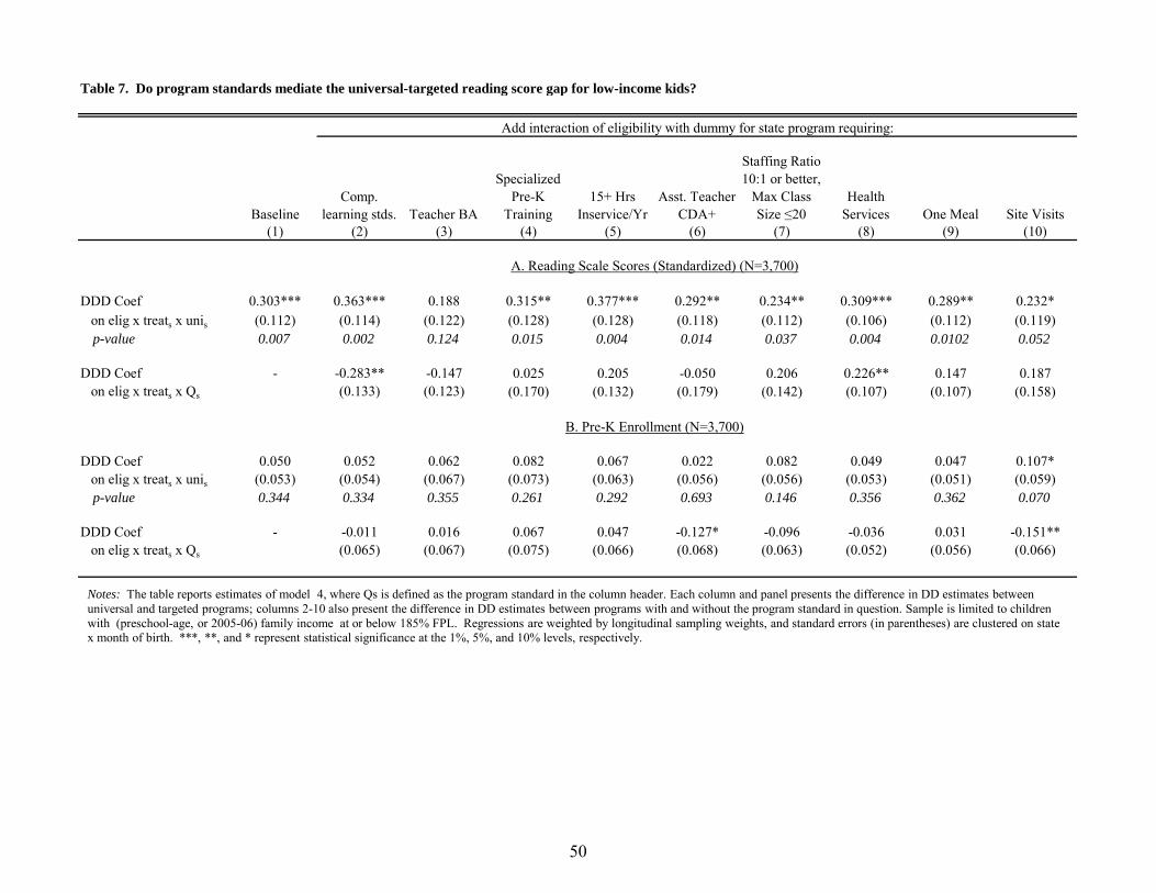
Table 7. Do program standards mediate the universal-targeted reading score gap for low-income kids?

BaselineComp.

learning stds. Teacher BA

Specialized Pre-K

Training15+ Hrs

Inservice/YrAsst. Teacher

CDA+

Staffing Ratio 10:1 or better,

Max Class Size ≤20

Health Services One Meal Site Visits

(1) (2) (3) (4) (5) (6) (7) (8) (9) (10)

DDD Coef 0.303*** 0.363*** 0.188 0.315** 0.377*** 0.292** 0.234** 0.309*** 0.289** 0.232* on elig x treats x unis (0.112) (0.114) (0.122) (0.128) (0.128) (0.118) (0.112) (0.106) (0.112) (0.119)

p-value 0.007 0.002 0.124 0.015 0.004 0.014 0.037 0.004 0.0102 0.052

DDD Coef - -0.283** -0.147 0.025 0.205 -0.050 0.206 0.226** 0.147 0.187 on elig x treats x Qs (0.133) (0.123) (0.170) (0.132) (0.179) (0.142) (0.107) (0.107) (0.158)

DDD Coef 0.050 0.052 0.062 0.082 0.067 0.022 0.082 0.049 0.047 0.107* on elig x treats x unis (0.053) (0.054) (0.067) (0.073) (0.063) (0.056) (0.056) (0.053) (0.051) (0.059)

p-value 0.344 0.334 0.355 0.261 0.292 0.693 0.146 0.356 0.362 0.070

DDD Coef - -0.011 0.016 0.067 0.047 -0.127* -0.096 -0.036 0.031 -0.151** on elig x treats x Qs (0.065) (0.067) (0.075) (0.066) (0.068) (0.063) (0.052) (0.056) (0.066)

Add interaction of eligibility with dummy for state program requiring:

A. Reading Scale Scores (Standardized) (N=3,700)

B. Pre-K Enrollment (N=3,700)

Notes: The table reports estimates of model 4, where Qs is defined as the program standard in the column header. Each column and panel presents the difference in DD estimates between universal and targeted programs; columns 2-10 also present the difference in DD estimates between programs with and without the program standard in question. Sample is limited to children with (preschool-age, or 2005-06) family income at or below 185% FPL. Regressions are weighted by longitudinal sampling weights, and standard errors (in parentheses) are clustered on state x month of birth. ***, **, and * represent statistical significance at the 1%, 5%, and 10% levels, respectively.

50

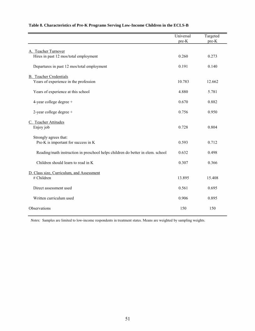
Table 8. Characteristics of Pre-K Programs Serving Low-Income Children in the ECLS-B

Universal Targeted pre-K pre-K

A. Teacher TurnoverHires in past 12 mos/total employment 0.260 0.273

Departures in past 12 mos/total employment 0.191 0.140

B. Teacher CredentialsYears of experience in the profession 10.783 12.662

Years of experience at this school 4.880 5.781

4-year college degree + 0.670 0.882

2-year college degree + 0.756 0.950

C. Teacher AttitudesEnjoy job 0.728 0.804

Strongly agrees that: Pre-K is important for success in K 0.593 0.712

Reading/math instruction in preschool helps children do better in elem. school 0.632 0.498

Children should learn to read in K 0.307 0.366

D. Class size, Curriculum, and Assessment# Children 13.895 15.408

Direct assessment used 0.561 0.695

Written curriculum used 0.906 0.895

Observations 150 150

Notes: Samples are limited to low-income respondents in treatment states. Means are weighted by sampling weights.

51

 

Notes: Data are from the ECLS-B and are restricted to children who, in 2005-06, were not eligible for free or reduced-price lunch. Panel A plots average pre-K enrollment rates at preschool age (in 2005-06) by age relative to the minimum age for kindergarten entry (2-month bins) for treated states with universal pre-K programs, treated states with targeted pre-K programs, and comparison states; see notes to Table 2 for lists of states in each of these groups. The dots in Panel B represent, separately for treatment states with universal programs and treatment states with targeted programs, the coefficients on interactions between a treatment dummy and a series of dummies for age relative to the minimum age for kindergarten entry (2-month bins) from a regression that allows for direct effects of each of these (sets of) variables. The dependent variable is a dummy for pre-K enrollment at preschool age (in 2005-06), and the interaction with the dummy for missing eligibility by 1 to 2 months is omitted to identify the interaction coefficients. The capped vertical lines represent 95% confidence intervals, with standard errors clustered on state by month of birth.

 

.1.2

.3.4

.5.6

.7Fr

actio

n

-4 -2 0 2 4 6Age (in mos.) relative to required K entry age

Comparison states

Universal states

Targeted states

A. Means

0.2

.4.6

-4 -2 0 2 4 6Age (in mos.) relative to required K entry age

Universal 95% C.I. Targeted 95% C.I.

B. Treatment-Comparison Difference

Figure A1. Prekindergarten Enrollment by Age and State Treatment Status:Not Low-Income Children

52

 

Notes: Data are from the ECLS-B and are restricted to children who, in 2005-06, were eligible for free or reduced-price lunch. Panel A plots average standardized math scores at preschool age (in 2005-06) by age relative to the minimum age for kindergarten entry (2-month bins) for treated states with universal pre-K programs, treated states with targeted pre-K programs, and comparison states; see notes to Table 2 for lists of states in each of these groups. The dots in Panel B represent, separately for treatment states with universal programs and treatment states with targeted programs, the coefficients on interactions between a treatment dummy and a series of dummies for age relative to the minimum age for kindergarten entry (2-month bins) from a regression that allows for direct effects of each of these (sets of) variables. The dependent variable is a standardized math score at preschool age (in 2005-06), and the interaction with the dummy for missing eligibility by 1 to 2 months is omitted to identify the interaction coefficients. The capped vertical lines represent 95% confidence intervals, with standard errors clustered on state by month of birth. 

-1-.

8-.

6-.

4-.

20

.2.4

Stan

dard

dev

iatio

ns

-4 -2 0 2 4 6Age (in mos.) relative to required K entry age

Comparison states

Universal states

Targeted states

A. Means

-.5

0.5

11.

5-4 -2 0 2 4 6

Age (in mos.) relative to required K entry age

Universal 95% C.I. Targeted 95% C.I.

B. Treatment-Comparison Difference

Figure A2. Preschool-Age Math Scores by Age and State Treatment Status:Low-Income Children

53

 

Notes: The dependent variable is standardized socio-emotional score at preschool age (in 2005-06). For further description, see notes to Figure A2.

-.6

-.4

-.2

0.2

.4St

anda

rd d

evia

tions

-4 -2 0 2 4 6Age (in mos.) relative to required K entry age

Comparison states

Universal states

Targeted states

A. Means

-1-.

50

.51

-4 -2 0 2 4 6Age (in mos.) relative to required K entry age

Universal 95% C.I. Targeted 95% C.I.

B. Treatment-Comparison Difference

Figure A3. Preschool-Age Socio-emotional Scores by Age and State Treatment Status:Low-Income Children

54

 

Notes: The dependent variable is standardized reading score at preschool age (in 2005-06), and the ECLS-B sample is restricted to children who, in 2005-06, were not eligible for free or reduced-price lunch. For further description, see notes to Figure A2. 

 

 

-.4

-.2

0.2

.4.6

.8St

anda

rd d

evia

tions

-4 -2 0 2 4 6Age (in mos.) relative to required K entry age

Comparison states

Universal states

Targeted states

A. Means

-.5

0.5

-4 -2 0 2 4 6Age (in mos.) relative to required K entry age

Universal 95% C.I. Targeted 95% C.I.

B. Treatment-Comparison Difference

Figure A4. Preschool-Age Reading Scores by Age and State Treatment Status:Not Low-Income Children

55

 

Notes: The ECLS-B sample is restricted to children who, in 2005-06, were not eligible for free or reduced-price lunch. For further description, see notes to Figure A2. 

 

   

-.4

-.2

0.2

.4.6

.8St

anda

rd d

evia

tions

-4 -2 0 2 4 6Age (in mos.) relative to required K entry age

Comparison states

Universal states

Targeted states

A. Means

-.5

0.5

-4 -2 0 2 4 6Age (in mos.) relative to required K entry age

Universal 95% C.I. Targeted 95% C.I.

B. Treatment-Comparison Difference

Figure A5. Preschool-Age Math Scores by Age and State Treatment Status:Not Low-Income Children

56

 

Notes: The dependent variable is standardized socio-emotional score at preschool age (in 2005-06), and the ECLS-B sample is restricted to children who, in 2005-06, were not eligible for free or reduced-price lunch. For further description, see notes to Figure A2.

0.2

.4.6

.8St

anda

rd d

evia

tions

-4 -2 0 2 4 6Age (in mos.) relative to required K entry age

Comparison states

Universal states

Targeted states

A. Means

-1-.

50

.51

-4 -2 0 2 4 6Age (in mos.) relative to required K entry age

Universal 95% C.I. Targeted 95% C.I.

B. Treatment-Comparison Difference

Figure A6. Preschool-Age Socio-emotional Scores by Age and State Treatment Status:Not Low-Income Children

57

 

 

Notes: Figures are constructed analogously to those in Panel B of Figures 3, 4, A2, and A3, but also include as controls a vector of state fixed effects, dummies for month of assessment, and the background controls listed in the Panel B of Table 2. See notes to figures referenced for further details.

 

0.2

.4.6

.8

-4 -2 0 2 4 6Age (in mos.) relative to required K entry age

Universal 95% C.I.

Targeted 95% C.I.

Pre-K Enrollment

-.5

0.5

1

-4 -2 0 2 4 6Age (in mos.) relative to required K entry age

Reading Score

-.5

0.5

1

-4 -2 0 2 4 6Age (in mos.) relative to required K entry age

Math Score

-1-.

50

.5

-4 -2 0 2 4 6Age (in mos.) relative to required K entry age

Socio-emotional Score

Figure A7. Event Study Estimates with Controls:Low-Income Children

58

 

Notes: Figures are constructed analogously to those in Panel B of Figures A1, A4, A5, and A6, but also include as controls a vector of state fixed effects, dummies for month of assessment, and the background controls listed in the Panel B of Table 2. See notes to figures referenced for further details.

 

 

-.2

0.2

.4.6

.81

-4 -2 0 2 4 6Age (in mos.) relative to required K entry age

Universal 95% C.I.

Targeted 95% C.I.

Pre-K Enrollment

-.5

0.5

1

-4 -2 0 2 4 6Age (in mos.) relative to required K entry age

Reading Score (Standardized)

-.5

0.5

1

-4 -2 0 2 4 6Age (in mos.) relative to required K entry age

Math Score (Standardized)

-.5

0.5

1-4 -2 0 2 4 6

Age (in mos.) relative to required K entry age

Socio-emotional Score (Standardized)

Figure A8. Event Study Estimates with Controls:Not Low-Income Children

59

Appendix Table A1. Impacts on Cognitive Test and Socio-emotional Scores at Preschool Age: No Additional Controls

States:Children: Low income Not low income Low income Not low income

(1) (2) (3) (4)

Ineligible mean -0.645 0.056 -0.582 -0.102DD Coef. on eligible x treated state 0.199* -0.011 -0.071 -0.081

(0.114) (0.108) (0.089) (0.097)TSLS Coef. on pre-K enrollment 0.965* -0.070 -0.454

(0.546) (0.681) (0.604)OLS Coef. on pre-K enrollment 0.087 0.294*** 0.097 0.397***

(0.064) (0.076) (0.073) (0.075)

Observationsa 1,850 2,200 1,900 2,400

Ineligible mean -0.680 0.089 -0.642 -0.132DD Coef. on eligible x treated state 0.168 -0.056 -0.003 -0.057

(0.140) (0.096) (0.106) (0.095)TSLS Coef. on pre-K enrollment 0.815 -0.357 -0.021

(0.632) (0.628) (0.674)OLS Coef. on pre-K enrollment 0.175** 0.211*** 0.166** 0.339***

(0.078) (0.059) (0.074) (0.062)

Observationsa 1,850 2,200 1,900 2,400

Ineligible mean -0.438 0.123 -0.235 0.200DD Coef. on eligible x treated state 0.181 0.119 -0.112 -0.028

(0.140) (0.126) (0.133) (0.109)TSLS Coef. on pre-K enrollment 0.924 0.880 -0.775

(0.710) (1.012) (0.921)OLS Coef. on pre-K enrollment -0.043 0.038 -0.013 0.122*

(0.094) (0.066) (0.089) (0.062)

Observationsa 1,600 1,950 1,650 2,150

C. Socio-emotional Scores (Standardized)

no f.s.

Universal Targeted

A. Reading Scale Scores (Standardized)

no f.s.

B. Math Scale Scores (Standardized)

no f.s.

Notes: The DD coefficient is that on the interaction between a dummy for being eligible for kindergarten in 2006-07 (synonymous with a dummy for being eligible for pre-K in 2005-06 in a treatment state) and a dummy for being in a treated state from a regression that also includes dummies for state of residence, for month of assessment, and for month age five relative to the state kindergarten entry cutoff birthdate in 2006-07; see notes to Table 2 for description and listing of treatment and comparison states. The TSLS coefficient uses eligible x treated state as an instrument for pre-K enrollment in a specification with the same controls. Sample is limited to children who turn age 5 between 4 months after and 8 months before the kindergarten entry cutoff birthdate, and a child is considered low income if his (preschool-age, or 2005-06) family income is at or below 185% FPL. Means and regressions are weighted by longitudinal sampling weights, and standard errors (in parentheses) are clustered on state x month of birth. a rounded to the nearest 50. ***, **, and * represent statistical significance at the 1%, 5%, and 10% levels, respectively.

60

Appendix Table A2. Additional Robustness Tests on Baseline Difference-in-Differences Estimates:Pre-K Enrollment and Socio-Emotional Test Scores

States:Children: Low income Not low income Low income Not low income

(1) (2) (3) (4)

Baselinea 0.207 -0.004 0.017 -0.055(0.129) (0.097) (0.109) (0.090)

Age 2 scores as controlsb 0.200* 0.014 0.037 -0.027(0.120) (0.096) (0.102) (0.092)

Pre-K states only in comp. groupc 0.286** 0.008 0.079 -0.035(0.137) (0.101) (0.117) (0.095)

+/- 4 months from cutoff d 0.324** 0.080 0.016 -0.013(0.145) (0.103) (0.121) (0.102)

Low income: Maternal ed ≤ HS 0.205 -0.015 0.032 -0.075(0.138) (0.095) (0.104) (0.089)

Low income: ≤130% FPL 0.111 0.054 0.082 -0.092(0.146) (0.080) (0.111) (0.081)

Drop FL and TX 0.191 -0.007 0.047 -0.015(0.174) (0.129) (0.130) (0.094)

Baselinea 0.157 0.161 -0.119 -0.041(0.132) (0.121) (0.132) (0.105)

Age 2 scores as controlsb 0.172 0.150 -0.074 -0.035(0.141) (0.119) (0.137) (0.104)

Pre-K states only in comp. groupc0.201 0.284** -0.093 0.062

(0.148) (0.124) (0.144) (0.115)+/- 4 months from cutoff d 0.218 0.229 -0.156 -0.010

(0.161) (0.156) (0.166) (0.120)Low income: Maternal ed ≤ HS 0.186 0.176 -0.098 -0.024

(0.165) (0.123) (0.132) (0.118)Low income: ≤130% FPL 0.113 0.168 -0.039 -0.065

(0.169) (0.112) (0.162) (0.098)Drop FL and TX 0.157 -0.000 -0.134 -0.061

(0.168) (0.159) (0.160) (0.113)

Universal Targeted

A. Math Scale Scores (Standardized)

B. Socio-emotional Scores (Standardized)

Notes: The DD coefficient is that on the interaction between a dummy for being eligible for kindergarten in 2006-07 (synonymous with a dummy for being eligible for pre-K in 2005-06 in a treatment state) and a dummy for being in a treated state from a regression that also includes dummies for state of residence, for month of assessment, and for month age five relative to the state kindergarten entry cutoff birthdate in 2006-07. See Table 2 for a definition of treatment and comparison states. Unless otherwise given, sample is limited to children who turn age 5 between 4 months after and 8 months before the kindergarten entry cutoff birthdate, a child is considered low income if his (preschool-age, or 2005-06) family income is at or below 185% FPL, regressions are weighted by longitudinal sampling weights, and standard errors (in parentheses) are clustered on state x month of birth. a Additional controls include age at assessment, dummies for female, Hispanic, black non-Hispanic, low birth weight, non-English at home, mom has high school degree or less, and both biological parents in household. b Missing test scores imputed and indicated with dummy variables to maintain sample size. c Comparison states limited to those with state-funded pre-K programs in 2005-06 (AL, AZ, CA, CT, DE, KY, MN, MO, NM, NV, OH, OR, WA) d Sample is limited to children who turn age 5 between 4 months after and 4 months before the kindergarten entry cutoff birthdate. ***, **, and * represent statistical significance at the 1%, 5%, and 10% levels, respectively.

61

Appendix Table A3. Do program standards mediate the universal-targeted math and socio-emotional test score gaps for low-income kids?

BaselineComp.

learning stds. Teacher BA

Specialized Pre-K

Training15+ Hrs

Inservice/YrAsst. Teacher

CDA+

Staffing Ratio 10:1 or better,

Max Class Size ≤20

Health Services One Meal Site Visits

(1) (2) (3) (4) (5) (6) (7) (8) (9) (10)

DDD Coef 0.190 0.203 0.234 0.161 0.167 0.181 0.152 0.191 0.187 0.168 on elig x treats x unis (0.144) (0.139) (0.191) (0.213) (0.175) (0.155) (0.147) (0.145) (0.141) (0.156)

p-value 0.189 0.146 0.223 0.450 0.339 0.244 0.304 0.190 0.185 0.282

DDD Coef - -0.064 0.056 -0.059 -0.062 -0.040 0.114 0.039 0.030 0.058 on elig x treats x Qs (0.166) (0.193) (0.222) (0.182) (0.170) (0.180) (0.140) (0.147) (0.197)

DDD Coef 0.276* 0.265 0.306* 0.419** 0.275 0.233 0.313* 0.276* 0.257* 0.320* on elig x treats x unis (0.154) (0.176) (0.174) (0.165) (0.176) (0.158) (0.167) (0.154) (0.151) (0.178)

p-value 0.074 0.134 0.078 0.012 0.119 0.142 0.061 0.073 0.090 0.073

DDD Coef - 0.052 0.040 0.306 -0.004 -0.198 -0.105 -0.066 0.140 -0.109 on elig x treats x Qs (0.226) (0.171) (0.202) (0.169) (0.291) (0.207) (0.152) (0.151) (0.230)

Add interaction of eligibility with dummy for state program requiring:

A. Math Scale Scores (Standardized) (N=3,700)

B. Socio-emotional Scores (Standardized) (N=3,200)

Notes: The table reports estimates of model 4, where Qs is defined as the program standard in the column header. Each column and panel presents the difference in DD estimates between universal and targeted programs; columns 2-10 also present the difference in DD estimates between programs with and without the program standard in question. Sample is limited to children with (preschool-age, or 2005-06) family income at or below 185% FPL. Regressions are weighted by longitudinal sampling weights, and standard errors (in parentheses) are clustered on state x month of birth. ***, **, and * represent statistical significance at the 1%, 5%, and 10% levels, respectively.

62

Appendix Table A4. Do demographics mediate the universal-targeted test score gaps for low-income kids?

BaselineAge in Months Female

Black non-Hispanic Hispanic

Low Birth Weight

Maternal Ed. ≤ HS

Both Biological

Parents in HHNon-English

at Home(1) (2) (3) (4) (5) (6) (7) (8) (9)

DDD Coef 0.303*** 0.302*** 0.300*** 0.304*** 0.281** 0.303*** 0.303*** 0.295*** 0.294*** on elig x treats x unis (0.112) (0.115) (0.113) (0.113) (0.112) (0.112) (0.114) (0.113) (0.110)

DDD Coef - -0.001 0.053 0.143 0.014 0.165* 0.253** -0.151 0.044 on elig x treats x Xi (0.013) (0.098) (0.106) (0.105) (0.090) (0.103) (0.094) (0.115)

DDD Coef 0.190 0.190 0.183 0.191 0.188 0.192 0.190 0.188 0.197 on elig x treats x unis (0.144) (0.143) (0.144) (0.145) (0.149) (0.145) (0.145) (0.144) (0.145)

DDD Coef - -0.006 0.114 0.074 0.016 0.036 0.046 -0.036 0.127 on elig x treats x Xi (0.015) (0.105) (0.135) (0.124) (0.109) (0.114) (0.102) (0.122)

DDD Coef 0.276* 0.282* 0.276* 0.278* 0.224 0.275* 0.277* 0.276* 0.267* on elig x treats x unis (0.154) (0.154) (0.153) (0.153) (0.161) (0.155) (0.153) (0.155) (0.156)

DDD Coef - -0.034 0.046 0.238 0.143 -0.010 0.059 -0.023 0.279* on elig x treats x Xi (0.022) (0.132) (0.159) (0.150) (0.137) (0.174) (0.126) (0.143)

Add interaction of eligibility with:

A. Reading Scale Scores (Standardized) (N=3,700)

B. Math Scale Scores (Standardized) (N=3,700)

C. Socio-Emotional Scores (Standardized) (N=3,200)

63

Appendix Table A4 (cont'd). Do demographics mediate the universal-targeted test score gaps for low-income kids?

BaselineAge in Months Female

Black non-Hispanic Hispanic

Low Birth Weight

Maternal Ed. ≤ HS

Both Biological

Parents in HHNon-English

at Home(1) (2) (3) (4) (5) (6) (7) (8) (9)

DDD Coef 0.050 0.052 0.051 0.049 0.051 0.050 0.050 0.045 0.044 on elig x treats x unis (0.053) (0.053) (0.052) (0.052) (0.053) (0.053) (0.052) (0.052) (0.053)

DDD Coef - -0.007 -0.027 0.085 -0.029 0.019 -0.076 -0.107** -0.127** on elig x treats x Xi (0.007) (0.048) (0.052) (0.057) (0.056) (0.054) (0.049) (0.057)

D. Pre-K Enrollment (N=3,700)

Add interaction of eligibility with:

Notes: The table reports estimates of model 4 but substituting demographic and background characteristics for Qs; the relevant characteristic is given in the column header, and the specification also includes a a two-way interaction between the eligbility indicator and the demographic characteristic. Each column and panel presents the difference in DD estimates between universal and targeted programs; columns 3-9 also present the difference in DD estimates for individuals with and without the demographic characteristic (the column 2 interpretation is slightly different due to the continuous nature of the characteristic). Sample is limited to children with (preschool-age, or 2005-06) family income at or below 185% FPL. Regressions are weighted by longitudinal sampling weights, and standard errors (in parentheses) are clustered on state x month of birth. ***, **, and * represent statistical significance at the 1%, 5%, and 10% levels, respectively.

64