dmrb volume 12 section 2 part 1 - traffic appraisal in
TRANSCRIPT
DESIGN MANUAL FOR ROADS AND BRIDGES
0
VOLUME12 TRAFFIC APPRAISAL OF ROADS SCHEMES
SECTION 2 TRAFFIC APPRAISAL ADVICE
PART 1
TRAFFIC APPRAISAL IN URBAN AREAS
SUMMARY
The purpose of this advice is to review the current best practice for urban traffic appraisal techniques in the context of trunk road assessment, and to extend the general methods set out in the Traffic Appraisal Manual (TAM) to the urban setting and the more congested inter-urban situations which involve complex traffic mteractions.
INSTRUCTIONS FOR USE
This is a new document to be incorporated into the Manual.
1. Insert DMRB 12.2.1 into Volume 12 at Section 2 in Binder 12a.
2. Archive this sheet as appropriate.
May 1996
a DESIGN MANUAL FOR ROADS AND BRIDGES
VOLUME 12 TRAFFIC APPRAISAL OF ROADS SCHEMES
Section 1 lhftk Appraisal Manual
Part 1 The Application of Traffic Appraisal to Trunk Road Schemes
Section 2 Traffic Appraisal Advice
Part 1 Traffic Appraisal in Urban Areas
May 1996
Traffic Appraisal in Urban Areas
THE HIGHWAYS AGENCY
THE SCOTTISH OFFICE DEVELOPMENT DEPARTMENT
THE WELSH OFFICEY SWYDDFA GYMREIG
THE DEPARTMENT OF THE ENVIRONMENT FORNORTHERN IRELAND
THE DEPARTMENT OF TRANSPORT
The purpose of this advice is to review the current best practice for urban traffic appraisaltechniques in the context of trunk road assessment, and to extend the general methods setout in the Traffic Appraisal manual (TAM) to the urban setting and the more congested inter-urban situations which involve complex traffic interactions.
Volume 12 Section 2 Part 1 Registration of Amendments
REGISTRATION OF AMENDMENTS
Amend No
Page No Signature & Date of incorporation of amendments
Amend No
Page No Signature & Date of incorporation of amendments
May 1996
Registration of Amendments
Volume 12 Section 2 Part 1
Amend No
Page No
REGISTRATION OF AMENDMENTS
Signature & Date of incorporation of amendments
Amend No
Page No Signature & Date of incorporation of amendments
May 1996

DESIGN MANUAL FOR ROADS AND BRIDGES
0
VOLUME 12 TRAFFIC APPRAISAL OF ROADS SCHEMES
SECTION 2 TRAFFIC APPRAISAL ADVICE
PART 1
TRAFFIC APPRAISAL IN URBAN AREAS
Contents
Chapter
1. Introduction and Contents
2. Modelling Overview - Objectives and Framework
3. Data Requirements
4. Traffic Model Development
5. Traffic Forecasting
6. Use of Traffic Model Outputs in Scheme Appraisal
7. Enquiries
Appendices
A I3 C D E F G H
Report of Traffic Survey Local Model Validation Report Forecasting Report The Use of Sub-periods and Time Slices Speed-flow Relationships The Application of Peak Spreading Growth Constraint Techniques Convergence
May 1996 Traffic Appraisal Advice
L ,’ ~
Traffic Appraisal
in Urban Areas
Volume 12 Section 2 Part 1 Traffk Appraisal in Urban Areas
Chapter 1 Introduction and Contents
0
1
1.1
1.1.1
1.1.2
0
1.1.3
1.1.4
1.1.5
a
1.1.6
1.1.7
Introduction and Contents
BACKGROUND
The recommended practice for the appraisal of trunk road schemes is set out in the Traffic Appraisal Manual (TAM) - Volume 12 Section 1 of the Design Manual for Roads and Bridges (DMRB ~12~1). The procedures contained in that document relate to trunk roads in England in rural, inter-urban and urban locations, although in practice the document has been used as a reference document by other overseeing organisations, with the predominant emphasis being towards the first two of these road types.
In 1986 a report entitled ‘Urban Road Appraisal’, containing recommendations for the assessment of urban trunk road schemes, was issued by the Standing Advisory Committee on Trunk Road Assessment (SACTRA) . A number of the suggestions were accepted for immediate implementation or were identified as needing further research. Subsequently the techniques employed in urban traffic appraisal have continued to evolve to meet developing needs.
The purpose of this advice is to review the current best practice for urban traflc appratial techniques in the context of trunk road assessmeut, and to extend the general methods set out in TAM and its Scottish counterpart STEAM to the urban setting. Much of the TAM advice that is common to both inter- urban and urban road schemes is assumed, and references to that advice are given where appropriate. Emphasis is given to areas where TAM and STEAM are not sufficiently specific about traffic assessment in urban areas, or where advice about particular aspects of urban traffic appraisal are missing altogether. Ongoing developments are noted, where appropriate.
In this Advice Note, references are generally given to the COBA Manual and TAM. Comparable advice can usually be found in the NESA Manual and in STEAM. Where this is not the case, the advice in COBA and TAM should be adopted in Scotland. Other references to COBA should be interpreted as applying to NESA.
While reference is made throughout this document to ‘urban’ areas, the methods described will ofterz be applicable to the appraisal of road schemes on the periphery of urban areas, and in the more congested inter-urban situat.!ons (partz*cuhrly those involving complex traflc interaction).
The main work in drafting this advice was completed before receipt of the report by SACTRA entitled “Trunk Roads and the Generation of Traffic”, and its publication in December 1994. A formal response, supplemented by an Advice Note giving Guidance on the modelling of Induced Traffic, was issued by the Government in December 1994 and research commissioned into several aspects arising from the SACTRA report. The most relevant results of the research - into peak spreading, traffic growth constraint techniques and convergence requirements for traffic assignment models have been reported in appendices F, G & H of this advice.
This advice and the Guidance on Induced Traffic are intended to be complementary. Until the latter is published in DMRB format (as Volume 12 Section 2 Part 2) it can be obtained from HETA Division 76 Marsham Street London SWlP 4DR.
May 1996 Traffic Appraisal Advice l/l

Chapter 1 Introduction and Contents
Volume 12 Section 2 Part 1 Traffic Appraisal :in Urban Areas
1.2 CONTEXT
1.2.1 The issues surrounding the traffic appraisal of trunk road schemes in urban areas should be seen in the context of the overseeing organisations’ responsibilities and their overall requirements for scheme assessment. Some information about this is given in Chapter 1 of TAM, but a fuller description is given below for convenience of presentation.
Responsibilities
1.2.2 The Department of Transport (DOT) is responsible for the network of trunk roads (including motorways) in England. This system was set up in 1936 to serve long distance through traffic. Similar arrangements apply in Northern Ireland, Wales and Scotland. Maintenance and improvement of this network (implemented in England through the Highways Agency) must meet the following aims:
l assist economic growth and efficiency by providing an effective road network
l support Government policies on economic growth and competitiveness
l conserve or enhance the environment by striking a balance between any environmental loss associated with the construction or improvement of roads and the overall benefits
l enhance road safety through improvements to the trunk road network to contribute to the Government’s target of reducing road casualties by a third by the year 2000
l maintain and manage the road network in a cost-effective manner while making the best use of the existing network.
1.2.3 Local highway authorities are responsible for the remainder of the road network and the prime responsibility for ensuring that local road investment meets its objectives rests with them. However, improvements to local highway networks that are of more than local importance can be supported by Central Government through Transport Supplementary Grant (TSG) in England and Wales. To ensure that schemes supported in this way provide good value for money, the Government attaches considerable importance to achieving a consistent approach to their traffic and economic appraisal.
Types of Scheme
1.2.4 Because of the nature of lhe trunk road network, many of the improvement schemes for which the overseeing organisations are responsible represent major investments with long lives. They are generally inter-urban or peri-urban in nature. However, they often form an integral part of local highway networks and serve local communities, and these functions must also be taken into account.
1.2.5 Most local highway authority schemes are smaller and many involving traffic management, parking, etc. are relatively short term in nature. However, their road schemes that are candidates for TSG support have tended to be larger schemes, more akin to those on trunk roads.
l/2 Traffic Appraisal Advice May 1996

Volume 12 Section 2 Part 1 Traffic Appraisal in Urban Areas
Chapter 1 Introduction and Contents
1.2.6
1.2.7
1.2.8
1.2.9
General Appraisal Requirements
One of the key requirements of scheme appraisal is that it should provide a robust and consistent basis for decision making. There is no case for a more elaborate analysis which reduces consistency with only marginal benefits in terms of robustness. An analysis that reduces robustness with only marginal benefits in terms of consistency is also not recommended. For this reason the quality of an appraisal should not be judged by the size of its traffic model, nor by its apparent sophistication, but by the speed and efficiency with which it can provide the information needed to make and justify decisions. The use of more sophisticated methods can only be justified if they provide a significant reduction in the risk of wrong decisions being made. It is also an important requirement that the work of appraisal itself should provide good value for money. This provides a further reason to avoid unnecessary, often peripheral, detail _
While the primary purpose of traffic assessment is to inform decisions, it is also important that those decisions should be demonstrably soundly based. The need to present scheme assessments to the public at Public Consultation and at Public Inquiry is a key consideration in the Department of Transport’s approach to appraisal. However, traffic forecasting can never be precise, and should not be presented as such, because it involves assumptions about the future and about the behaviour of people.
In addition, the overall scheme preparation process must assess and reflect economic and environmental impacts, with operational considerations also acting as a constraint. The traffic appraisal must serve this objective, and is not an end in itself.
The above factors have led the overseeing organisations to develop a broadly standardised approach to traffic assessment. The emphasis of this approach is on good decision making, rather than on detail. Much of the work of traffic appraisal makes use of standard methods and values to ensure consistency between one appraisal and another. This is of obvious value to those who must make decisions on different types of schemes in a range of locations. It is also of value to those outside the overseeing organisations who need to understand the methods used.
The Stages of Trunk Road Assessment
1.2.10 Prior to proposals for a new or upgraded trunk road scheme entering a programme of schemes it is necessary to undertake a route appraisal or area wide smdy to identify the most appropriate approach to resolving problems. Particularly in urban areas, such studies will need to have regard to possible alternatives to road improvements. These alternatives might, for instance, include packages of measures such as constraints on traffic growth (eg through parking controls), traffic management / ‘calming’ <arid improvements to public transport. However, given the role of trunk roads in catering for longer-distance traffic, the ability of such alternatives to fully meet the needs in a congested location may well be limited, although they may be more likely to play a complementary role. Some aspects of multi-modal appraisal are covered in TAM Chapter 17 and its associated Appendix.
1.2.11 Assuming that the need for a road scheme has been identified, as part of the appropriate solution and having entered the programme, trunk road scheme proposals are assessed at various stages of their development. The overseeing Departments have developed appraisal methods and procedures to ensure that the correct level of validated information is available to enable decisions to be made and justified at each stage.
May 1996 Traftic Appraisal Advice l/3
Chapter 1 Volume 12 Section 2 Introduction and Contents Part 1 Traffic Appraisal in Urban Areas
1.2.12 Although the process of data collection, model building and analysis is continuous throughout scheme a
preparation, results are required in England and Wales to inform discussions at three specific stages, namely:
0 pre-public consultation;
0 preferred route announcement stage; and
0 order publication stage.
Equivalent reporting stages apply in Scotland and Northern Ireland. As scheme preparation progresses, the methods and data used sometimes need to be refined to suit the required focus.
1.2.13 It is left to the local teams in the Highways Agency in England and specialists in other overseeing organisations to decide upon the traffic appraisal methods for specific schemes, guided by the advice contained in TAM. The local teams in England must comply with three particular requirements that are mandatory for traffic appraisal on trunk roads. These are:
0 production of a Traffic Study Data Base; 0
0 production of a Local Model ‘Validation Report; and
0 production of a Forecasting Report.
These require approval by technical staff within the overseeing organisations, or in England TSD division within the Highways Agency. The technical requirements to be addressed in these documents are set out in Chapters 3, 4 and 5.
1.2.14 Guidance on the level of environmental appraisal required at the key stages in the development of a trunk road scheme, and on the requirements for reporting the effects on the environment, is provided in Volume 11 of the Design Manual for Roads and Bridges.
Trunk Road Appraisal in Urban Areas
1.2.15 Although the problems of urban traffic appraisal are generally more complex, the general principles relating to the assessment of other types of trunk road scheme still apply. 0
1.2.16 However, analytical techniques that work reliably in rural areas are not always appropriate for traffic appraisal in more congested urban networks, and a variety of methods have been developed for use in these situations. Such procedures should be considered when it is clear that simpler approaches would give misleading results. An urban setting does not in itself justify the use of more sophisticated methods. The justification is the necessity to make sound decisions on the scheme involved. Examples of situations in which these more sophisticated methods may be required are given in Chapter 2.
Area Models
1.2.17 The advice presented here is in the context of models developed to appraise specific trunk road schemes. However much of it will be applicable to the development of ‘general purpose’ models developed in particular areas (eg conurbations) to enable a variety of analyses to be undertaken. This is of particular importance where such models are to be used for, or to provide inputs for, the appraisal of Trunk Road schemes. In those circumstances the requirements of paragraph 1.2.13 must be met by the general purpose model.
l/4 Traffic Appraisal Advice May 1996
Volume 12 Section 2 Part 1 Traffic Appraisal iu Urban Areas
Chapter 1 Introduction and Contents
1.3 IMPLEMENTATION IS!WES
1.3.1 This document supersedes the consultation draft version dated February 1994. It should be used forthwith on all urban trunk road schemes where the appraisal has only recently started, and on other schemes where there are complex traffic interactions. The methodology is recommended for other similar schemes unless a stage has been reached at which in the opinion of the Overseeing Organisation, its use would result in an unacceptable delay to progress.
1.3.2 Design organisations should confirm its application to particular schemes with the Overseeing Organisation.
1.3.3
0
1.3.4
This advice reviews the current best practice for urban traffic appraisal techniques in the context of trunk road assessment, and extends the general methods set out in the Traffic Appraisal Manual (TAM) to the urban setting and the more congested inter-urban situations which involve complex traffic interactions. It sets out some details of concepts involved in the appraisal of highway schemes and of the Overseeing Organisations’ key requirements on the timing and reporting of appraisals. For highway schemes costing less than &Sm alternative less sophisticated techniques may be more appropriate.
Guidance on the techniques available for rural applications are contained in the ‘T’raffi,c Appraisal Manual (TAM (DMRB 12.1)). Guidance on the evaluation of non-economic elements of highway proposals is contained in Volume 11 of the DMRB - Environmental Appraisal.
May 1996 Traffic Appraisal Advice l/5
Chapter 1 Introduction and Contents
Volume 12 Section 2 Part 1 Traffk Appraisal in Urban Areas
1.4 STRUCTURE OF THIS ADVICE and DETAILED CONTENTS
1.4.1 The remainder of this advice describes those traffic appraisal procedures that are considered to be most relevant to urban areas. Chapter 2 gives an overview of the main issues involved, and is intended to be a guide to senior managers when formulating the traffic appraisal framework for a particular road scheme.
1.4.2 Later chapters cover the various procedures in greater technical detail. Chapter 3 reviews the types of data needed in urban traffic appraisal, with particular reference to the reasons for collecting each data type. Chapter 4 deals with the construction of a base year traffic model, while Chapter 5 discusses the main techniques for forecasting future traffic levels in urban areas.
1.4.3 Chapter 6 outlines the other types of scheme assessment (economic, operational, environmental) that use outputs from the traffic appraisal.
1.4.4 A series of appendices contain technical material considered too detailed for inclusion in the main body of the text _
1.4.5 The following conventions are used to convey emphasis:
Text boxes contain important recommendations. If these are not followed analysts will need to provide rigorous justification for the course of action taken.
Italicised text k used to highlight other matters of imponiznce to which attention needs to be drawn.
l/6 Traffic Appraisal Advice May 1996

Volume 12 Section 2 Part 1 Traffic Appraisal in Urban Areas
Chapter 1 Introduction and Contents
Detailed Contents
Chapter 1
1.1
1.2
1.3
1.4
1.5
Chapter 2 MODELLING OVERVIEW - OBJECTIVES AND FRAMEWORK
2.1 2.2 2.3 2.4 2.5 2.6 2.7 2.8 2.9 2.10 2.11 2.12
Chapter 3
3.1
3.2
INTRODUCTION and CONTENTS
Background
Context
1.2.2 ff Responsibilities 1.2.4 ff Types of Scheme 1.2.6 ff General Appraisal Requirements 1.2.10 ff The Stages of Trunk Road Assessment 1.2.15 ff Trunk Road Appraisal i,n Urban Areas 1.2.17 Area Models
Implementation Issues
l/l
l/2
l/2 l/2 l/3 l/3 l/4 l/4
l/5
Structure of this Advice and Detailed Contents l/6
Glossary of Abbreviations and Index of Cross References to TAM and COBA l/12
Page
General 2/l Characteristics of Urban Road Networks 2/l Model Structure and Requirements 212 Model Area 213 Model Time Periods 214 Travel Purposes 2/s Vehicle Types 216 Base and Forecast Years 217 Forecasting Methods 217 Data Requirements and Availability 2/a Software Requirements 219 Other Aspects of Scheme Appraisal 2/10
2.12.2 ff Economic Appraisal 2/10 2.12.5 ff Application to Scotland 2110 2.12.7 ff Environmental Appraisal 200
DATA REQUIREMENTS
General
Page
3/l
Types of Data Required 312
3.2.4 ff 3.2.17 ff 3.2.19 ff 3.2.24 3.2.25 ff 3.2.30 ff 3.2.32 ff 3.2.34 ff
Origin to Destination Data 312 Registration Number Surveys 315 Count Data 316 Network Data 317 Journey Time Measurements 317 Queue Length and Delay Measurements 318 Other Geometric and Operational Data 318 Parking Supply Data 319
Page
May 1996 Traffic Appraisal Advice l/7
Chapter 1 Volume 12 Section 2 Introduction and Contents Part 1 Traffic Appraisal in Urban Areas
3.3
3.4
3.5
3.2.34 ff Public Transport Data
3.2.34 Planning Data
Use of Existing Data
Data Processing and Analysis
Reporting Requirements
Chapter 4 TRAFFIC MODEL DEVELOPMENT Page
4.1 General
4.1.3 ff Model Structure 4.1.7 Validation Principles 4.1.8 ff Software Requirements 4.1.13 ff Study Area and Zoning System 4.1.20 ff Zone Size
4.2 Network Description 416
4.2.7 ff Parking 418 4.2.9 Network Checking 418
4.3 Base Year Trip Matrices 4/10
4.3.6 ff Matrix Construction Methods 4.3.13 Corridor Factors 4.3.14 ff Motorways 4.3.16 Transposing Observed Movements 4.3.17 ff Matrix Infilling Methods 4.3.28 ff Matrix Manipulation 4.3.30 ff Matrix Updating Methods 4.3.42 ff Trip Matrix Validation
4.4 Traffic Assignment 4118
4.4.1 ff Assignment Methods 4118
4.4.6 ff Other Features of Assignment Models 4120 4.4.9 ff Flow Metering and Blocking Back 4121 4.4.11 ff Route Choice Generalised Cost Coefficients 4121 4.4.14 ff Speed-flow Relationships 4122
4.4.19 ff Model Convergence 4123 4.4.25 ff Treatment of Different Vehicle Types 4125 4.4.29 ff Assignment Model Calibration 4125 4.4.34 ff Assignment Model Validation 4127
4.4.42 ff VaIidation Acceptability Guidelines 4128 4.4.44 ff Presentation of Comparisons 4129
4.5 Reporting Requirements 4130
4/l
412 413 413 a 414 416
4/11 4112 4112 4113 4113 4/l!? 4115 4117 a
l/8 Traffic Appraisal Advice May 1996
Volume 12 Section 2 Part 1 Traffic Appraisal in Urban Areas
Chapter 1 Introduction and Contents
l Chapter 5
5.1
5.2
5.3
5.4
5.5
5.6
5.7
5.8
Chapter 6
6.1
6.2
6.3
6.4
6.5
0 Chapter 7 ENQUIRIES
TRAFFIC FORECASTING Page
Elements of Forecasting 5/l
Forecast Years 5/l
Future Year Networks 512
5.3.3 ff ‘Do Minimum’ Networks 512
5.3.6 ff ‘Do Something’ Networks 513
Traffic Demand Forecasts 513
5.4.3 ff National Trip End Model 513
5.4.8 ff Growth Factors from Higher Tier Models 516 5.4.10 NRTF Growth Factors 516
Assignment 517
5.5.2 Route Choice Criteria 517
5.5.3 Convergence Requirements 517
5.5.4 Assignment Model Checks 518
5.5.5 Overloaded Junctions S/8
Initial Adjustments to Demand 519
5.6.1 ff Parking Demand 519
5.6.3 Peak Spreading 519
Constraints to Growth 500
Reporting Requirements 5/12
USE OF TRAFFIC MODEL OUTPUTS IN SCHEME APPRAISAL Page
General 6/l
Economic Appraisal 6/l
6.2.2 ff Fixed and Variable Matrix Methods 6/l 6.2.6 ff COBA 612
6.2.1.5 ff URECA 614
Delays at Roadworks 616
6.3.1 ff QUADRO and alternatives 616
Environmental Impact Assessment 618
6.4.3 ff Traffic Flow 618 6.4.5 ff Traffic Composition 618
6.4.7 Traffic Speed 619
Operational Appraisal and Scheme Design 619
6.5.1 ff Operational Assessment 619 6.5.3 ff Geometric Design 619 6.5.6 Pavement Design 6110
Page 7/l
May 1996 Traffic Appraisal Advice l/9
A
B
C
D
E
F
G
H
Appendices Page
Report of Traffic Survey
Local Model Validation Report
Forecasting Report
The Use of Sub-periods and Time Slices
Speed-flow Relationships
The Application of Peak Spreading
Growth Constraint Techniques
Convergence
A/l
B/l
C/l
D/l
El
F/
G/
H/l
Chapter 1 Introduction and Contents
Volume 12 !3ectho 2 Part 1 Traffic Appraisal in Urban Areas
l/10 Traffic Appraisal Advice May 1996
Volume 12 Section 2 Part 1 Traffic Appraisal in Urban Areas
Chapter 1 Introduction and Contents
4.1
4.2
3.1
a 4.1
4.2
5.1
Al
A2
Bl
a B2
B3
B4
B.5
B6
Cl
Dl
D2
Tables
Summary of Convergence Criteria
Assignment Validation Acceptability Guidelines
Figures
Acceptability of Trip Reversal
Preparation of Trip Matrices
Choice of Assignment Model
Trip Forecasting Process
Figures to Appendices
Presentation of Junction Flows
Presentation of Desire Line Data
Desire Line Comparisons - An example
Journey Time Validation - An example
Journey Time Validation - An example
Plot of Flow Differences - An example
Base Year Link Flow Validation - An example
Base Year Link Flow Validation - An example
Load Relief Diagram - An example
Presentation of Flow Profiles - An example
Derivation of Time Slice Data
Page
4124
4128
Page
314
419
4120
514
Page
Al3
Al4
B/5
B/6
B/7
B/8
B/9
B/IO
Cl4
D/3
D/4
May 1996 Traffic Appraisal Advice l/11
Chapter 1 Introduction and Contents
Volume 12 Section 2 Part 1 Traffic Appraisal in Urban Areas
1.5 GLOSSARY OF ABBREVIATIONS AND CROSS REFERENCES TO TAM AND COBA
AADT AAHT ACTRA ARCADY ATC CBA CBD CFREE COBA ClOPREP DM DMRB DOT DS
ERICA FR FYRR GDP GEH GMTU HA HEN1 HEN2 HETA HGV IHMS LGV LMVR MATVAL MCC ME2 MOVA MSA msa NESA NFAF NPV NRTF NTEM NTS
Annual Average Daily Traffic Flow Annual Average Hourly Traffic Flow Advisory Committee on Trunk Road Assessment Computer program for the design of roundabouts Automatic Traffic Count Cost Benefit Analysis Central Business District Coba FREe format data Entry program Cost Benefit Analysis computer program and associated manual Coba Interactive data PREParation program Do Minimum situation Design Manual for Road and Bridges Department of Transport Do Something situation former Environmental Appraisal Manual (now available as Volume 11 of DMRB) Economic Assessment Report Eastern Region Interview data Comparison and Analysis computer program Forecast Report First Year Rate of Return Gross Domestic Product A form of Chi-squared statistic defined in para 4.4.42 Greater Manchester Transportation Unit Highways Agency Highways Economic Note No.1 - Road Accident Costs Highways Economic Note No.2 - VOT and VOC Highways Economic and Traffic Appraisal Division DOT Heavy Goods Vehicle Integrated Highways Maintenance System Light Goods Vehicle Local Model Validation Report Sub-routine within ROADWAY computer program Manual Classified Count Matrix Estimation by Maximising Entropy technique Computer program for vehicle actuated signals Method of Successive Averages Million Standard Axles Network Evaluation from Survey and Assignments for use instead of COBA in Scotland National Forecast Adjustment Factor Net Present Value National Road Traffic Forecasts National Trip End Model National Travel Survey
l/12 Traffic Appraisal Advice May 1996
Volume 12 Section 2 Part 1 Traffic Appraisal in Urban Areas
Chapter 1 Introduction and Contents
a O/D O-D OGV OGVl OGV2 OPR OSCADY OSGR PC PCU PH/PP PHV PIA PICADY PR PSV PTRC PVB PVC PVY QDN QUADRO RCPI RDGRAV2 RDMERG ROADWAY RPF RPX’ RS SACTRA STC STEAM SUE TAM TRANSYT TRL TRRL TSD TSG URECA VIC voc VOT WLCM
Origin to Destination Origin to Destination Other Goods Vehicle Other Goods Vehicle - Category 1 Other Goods Vehicle - Category 2 Order Publication Report Computer program for the design of traffic signal settings Ordnance Survey Grid Reference Public Consultation Passenger Car equivalent Unit Peak Hour to Peak Period ratio Percentage Heavy Vehicles (OGVl + OGV2 + PSV) Personal Injury Accident Computer program for assessing the capacity and design of priority junctions Preferred Route stage Passenger Service Vehicle Planning Transportation Research and Computation (Int Association) or (Ed Services Ltd) Present Value of Benefits Present Value of Costs Present Value Year QUADRO DIVersion sub-routine/computer program Queues And Delays at ROadworks computer program Road Construction Price Index Sub-routine within ROADWAY Sub-routine within ROADWAY Traffic data assembly and assignment computer program Relative Price Factor Retail Price Index Road Safety Division of the DOT Standing Advisory Committee on Trunk Road Assessment STatistics “C” Division of the DOT Scottish Traffic and Environmental Appraisal Manual Stochastic User Equilibrium assignment procedure Traffic Appraisal Manual (soon to be reprinted as Volume 12 Section 1 of DMRB) Computer program for the optimisation of linked traffic signals Transport Research Laboratory (formerly TRRLJ Transport <and Road Research Laboratory Technical Services Division of the Highways Agency Transport Supplementary Grant URban Economic Appraisal computer program Volume to Capacity ratio Vehicle Operating Costs Value of Time Whole Life Cost Model
Further abbreviations are used in Appendix E and are defined in Tables in that Appendix.
May 1996 Traffic Appraisal Advice l/13
Chapter 1 Introduction and Contents
Volume 12 Section 2 Part 1 Traffic Appraisal in Urban Areas
This Advice makes the following specific references to TAM as reprinted in August 1991 and COBA 9. References to the latest edition of those documents can be deduced by reference to the following tables:-
This Advice TAM sub-section (August 1991) Superseded by
1.1. 1, 1.1.3, 1.2.13 & 2.126 General Reference 1.2. 1 Chapter 1 1.2.10 Chapter 17 & Appendix Al7 2.3. 4 Chapter 2 2.4. 1 Chapter 3 2.8. 3 Sub-Section 12.3 2.9. 2 Chapter 12 2.10.1 & 3. 2.2 Chapter 6 2.10.2 & 2.11.3 Sub-Sections 2.2 & 11.4 3. 2. 3 Sub-Sections 6.2 & 6.3 3. 2.16 Sub-Section 6.4 3. 2.18 Sub-Section 6.7 3. 2.19 Sub-Sections 6.5 & 6.6 3. 2.24 Sub-Section 6.8 4. 1. 7 Chapter 11 4. 1.11 Sub-Section 8.7 4. 1.13 Sub-Section 3.1 4. 1.14 Chapter 3 4. 1.17 Sub-Section 3.2 4. 3. 6 Sub-Sections 8.1, 8.2 & General 4. 3.20 Sub-Section 8.3 4. 3.40 Sub-Section 8.5 4. 3.43 Chapter 10, Sub-Sections 10.2 & 10.4 4. 3.45 Sub-Sections 6.12 & 11.4 4. 4.11 Sub-Section 9.6 4. 4.35 & 4. 4.44 Sub-Section 11.4 5. 1. 1 & 5. 2. 3 Sub-Section 12.3 5. 4. 7 Chapters 7 & 12 5. 5. 2 Sub-Sections 12.3 & 12.5 6. 5. 2 Chapter 13
This Advice
2. 6. 2 2. 7. 2 2. 8. 3 2.12. 2 3. 2.29 4. 4.14 to 4.4.17 5. 2. 2 5. 3.35 5. 7. 1 5. 7. 5 6. 2. 1 to 6. 2. 25 & 6. 4. 5
Appendices B, C, E & G
COBA 9
General Sub-Section 4.8 Sub-Section 4.4 General Sub-Section 5.10 General General Sub-Sections 1.2 & 3.4 General Sub-Section 6.4 General General
COBA 10 (Vol 13 of DMRB)
DMRB 13.1.4.7 DMRB 13.1.4.4
DMRB 13.1.5.10 & 11
DMRB 13.1.1.2 & 13.1.3.4
DMRB 13.1.6.4
l/14 Traffic Appraisal Advice May 1996

Volume 12 Section 2 Part 1 Traffic Appraisal in Urban Areas
Chapter 2 Modelling Overview
a 2
2.1
2.1.1
2.1.2
2.1.3
a
2.1.4
2.2
2.2.1
l 2.2.2
2.2.3
Modelling Overview - Objectives and Framework
GENERAL
This chapter provides an overview of the main issues regarding the use of urban trunk road traffic appraisal techniques, and guidance in setting modelling objectives.
It k essential to have a clear understanding of the ultimate scope and objectives of the appraisal before detailed analysk begins;. Poor understanding of the issues involved, and the adoption of inappropriate techniques, is likely to lead to delay and additional expenditure in scheme preparation, and confusion in the minds of those appraising the scheme.
For the majority of urban or peri-urban road schemes, the traffic appraisal will be sufficiently complex to warrant the use of computer modelling techniques. The main emphasis is therefore on the use and interpretation of such models. Despite any added complexity of urban traflc apprakal, the same criteria of accuracy and robustness used on inter-urban schemes continue to apply.
The description of urban traffic appraisal given below is intended to provide only a basic appreciation of the issues involved. These issues, together with the various methods employed in this type of appraisal, are discussed in greater detail in subsequent chapters.
CHARACTERISTICS OF WAN ROAD NETWORKS
One of the main sources of congestion in urban road networks is the higher frequency of road junctions, which is sometimes compounded by interaction between junctions. Such junctions usually control the capacity of the road system, and govern journey times and routes taken by drivers. Drivers may respond to this congestion by seeking alternative routes, including so-called ‘rat runs’, that were never intended to be used by through traffic. An additional complication is that operating characteristics of urban road networks, and therefore the main factors affecting route choice, can vary significantly by time of day (and sometimes also by season).
Other responses to congestion - and ones that are more difficult to deal with - involve drivers travelling at different times or in a different sequence, or travelling to similar facilities in less congested areas. As an alternative, they may choose to travel by public transport, and not use their car at all.
When road capacity is increased, by construction of new road space or by the introduction of traffic management measures, the opposite of these effects may sometimes occur. Traffic levels, or traffic growth rates, will then be above those that might otherwise have been expected, and congestion may return sooner than anticipated. Any road scheme in, near or through an urban area will be affected by these factors to a greater or lesser extent, and traffic appraisals for these schemes will need to take account of such issues. Comprehensive advice on appropriate techniques is provided in the Guidance on Induced Traffic published by the Department of Transport in December 1994, and this will be continued in its expected updates .
May 1996 Traffic Appraisal Advice 2/l

Chapter 2 Modelling Overview
Volume 12 Section 2 Part 1 Traffic Appraisal in Urban Are&-s
2.3 MODEL STRUCTURE AND REQUIREMENTS
2.3.1 The type and complexity of the traffic model required to carry out the appraisal will depend on the scale of the scheme proposed. For improvements to an isolated junction, where no appreciable re-routeing of traffic is anticipated, the traffic model might simply simulate the behaviour of traffic at the junction before and after implementation of the scheme, and so calculate changes to queue lengths and delays to traffic at various times of day. At the other extreme, major road schemes involving significant changes to travel patterns over a wide area will usually require a more complex simulation of people’s choices. This can be based on either incremental changes from an existing observed situation (known as a ‘pivot point model’) or full acceptance of a ‘synthetic’ model validated against the existing situation, but which otherwise discards the detailed observaGons. Schemes of intermediate size will require a model structure to suit the complexity and extent of the travel impacts likely to be involved.
2.3.2 The most complex type of model used in urban areas is sometimes referred to as a ‘comprehensive (or four stage) transport planning model’. In its most common form, this assumes that the decisions people make about travel can be separated into a sequence of combined or independent steps, for example:-
0 ‘Trip end estimation’ : sub-divides the area being studied into zones and calculates the number of a
journeys that begin and end in each zone, depending on its land use, socio-economic and car ownership characteristics;
0 ‘Trip distribution’: estimates the number of journeys between each pair of zones in the study area, depending on the separation between the zones (in terms of time and distance) and their relative generation and attraction potential;
0 ‘Modal split’: apportions the journeys between each pair of zones to different modes of travel, according to the relative attractiveness of using the alternative modes of travel (e.g. generalised costs); and
0 ‘Assignment’ : allocates the journeys between each pair of zones to one or more routes between the zones, using the appropriate mode of travel.
There are other types of higher tier model which can take account of other responses (e.g. changes in time of travel), but the direct application of these models to the appraisal of trunk road schemes will not often be appropriate. However, where network based models are available they can be used to assess strategic a re-assignment effects.
2.3.3 For trunk road apprakul, emphasis k placed on observed, rather than synthesised, movements and tra&‘ic forecasts are based on local growth factors applied to these observed movementi as far as possible. However, distrlbutiora and multi-modal eflects need to be &en into account if they are expected to be signz@icant. Therefore, for some trunk road appraisals in urban areas it may be necessary to include all of the above model elements. For example:
0 where a scheme is expected to have a significant impact on the pattern of trips between origins and destinations in the scheme area, simple matrix adjustment techniques, based on zonal trip end growth are unlikely to be adequate for forecasting future travel patterns, and a full trip distribution sub-model will usually be required; and
0 if a scheme is expected to have significant impact on the choice between travel modes, a modal split sub-model will usually be necessary.
The assignment sub-model usually has major significance in the appraisal of urban road schemes, and, except for simple junction improvements, will always be required.
a
212 Traffw Appraisal Advice May 1996

Volume 12 Section 2 Part 1 Traffic Appraisal in Urban Areas
Chapter 2 Modelling Overview
a 2.3.4 The Guidance on Induced Traffic provides an overview of the model structure required, when Induced
traffic is likely to be important and Chapter 2 of TAM provides an overview of the issues involved in designing a traffic study and carrying out traffic assessments for trunk road schemes. However, the TAM advice is not specifically related to schemes in urban areas, and this should be recognised when dealing with such schemes. Other aspects of the traffic model that need to be considered when specifying a traffic appraisal exercise are described below.
2.4 MODEL AREA
2.4.1 The definition of the study area required for a scheme appraisal is very important. It is defined here and in Chapter 3 of TAM as the area within which link flows or journey times or delays will be significantly affected by the implementation of the scheme. This means that for an urban apprakul, the study areu needs to be s@Tcient for the relkble modelling of significant traflc Jlow or journey time or de&y changes. Within that general principle, the main issues that must be considered when defining the study area are discussed below.
2.4.2 The scale of modelling required can usually be readily determined by considering the following issues:
0 the routes currently being used (or likely to be used in the future) by traffic affected by the scheme:
0 the areas where significant relief would be provided by the scheme;
0 the areas susceptible to significant disbenefits produced by any extra traffic induced by the scheme:
0 the impact of changes in traffic levels on both existing and new/improved roads in the areas affected; and
0 the area over which economic benefits are to be assessed.
Key aspects regarding these issues are discussed below. However, in general unless the effects can be quantified accurately over the life of the scheme, there is usually no point in extending the study area to pick up minor, but widespread, ripple effects in areas remote from the scheme, except where omitting the effect would introduce a significant bias.
2.4.3 If congestion in a corridor is severe, through traffic may be displaced into parallel corridors, or it may use secondary roads to avoid the worst bottlenecks. There may also be other induced responses to congestion such as re-timing, re-distribution, etc. and these may counteract rerouteing responses and affect net operating costs more severely and with fewer counter-balancing effects over a wider area than rerouteing responses _
2.4.4 Where a suitably validated higher tier, or regional model, exists it should be used to provide some indication of the extent of these strategic effects, and help determine the area of influence of the scheme. In the absence of such a model, the application of local expertise and judgement may be necessary, but can be difficult to defend at a later stage. It should also be remembered that attracting traffic back into the scheme corridor may lead to the diversion of other traffic movements onto routes relieved by the scheme itself. However, if there are strong grounds to suggest that there will be no strategic or induced
0
effects, there are considerable practical advantages in using a tightly localised network.
May 1996 Traffic Appraisal Advice 213
Chapter 2 Modelling Overview
Volume 12 Section 2 Part 1 Traffk Appraisal in Urban Areas
2.4.5
2.4.6
2.4.7
2.5
2.5.1
2.5.2
2.5.3
Whatever the impact of the scheme under consideration, general traffic growth in the scheme area, and network changes between the base and future years in the do-minimum, may lead to different patterns of congestion, and route& in the future. Whilst the study area should be wide enough to reflect these do- minimum changes, this may result in problems with convergence of the iterative process and the robust benefit estimation for the scheme. If the differences between the scheme and the do-minimum are significantly smaller than those between the base year and the do-minimum, it may be necessary to reduce the model area for the appraisal of the scheme, once the do-minimum situation has been modelled satisfactorily.
If a gravity model is to be used (e.g. for matrix infilling), it is important that the great majority of trips are contained within the model area and that the full interzonal cost should be calculated for external trips. These aims can be achieved by extending the size of the model area. If this is not feasible, then full interzonal costs can be determined by means of an external network with realistic link distances and times.
Finally, there may be development proposals in the vicinity of the scheme that are expected to generate traffic of major operational, economic or environmental significance; in some cases, these may account for all the local growth expected, and impose traffic flows on the network that have little in common with existing traffic movements. These should be modelled as set out in paragraphs 5.4.4 and 5.4.5 and the study area should be sufficiently wide to allow traffic associated with such developments to disperse through the road network in a realistic way.
MODEL TIME PERIODS
For rural roads, and other road schemes away from congested urban areas, it is usual to use a single ‘all- day’ traffic model, covering a 12- or 16-hour period. In congested urban areas the variation of travel times and costs through the day is more complex. When modelling these areas it is lls@,v necessary to break the day down into separate model periods covering AM, PM and inter-peak periods, for weekdays. It may also be necessary to construct separate models for off-peak periods and weekends. For economic appraisal purposes, each model period is considered to contribute a proportion of the annual scheme benefits, and model periods need to cover those parts of the day in which significant benefits are likely to accrue. Similarly, the traffic flows input to the environmental appraisals are sometimes required for the whole day, and this may mean aggregating traffic flows from the various short period models into a longer period and, possibly, factoring the model results to cover parts of the day that have not been modelled _
As different circumstances surround each scheme, some judgement has to be made as to the start time and duration of the periods modelled. These should be chosen to represent periods of distinctly dimrent traflc condihons. It is often helpful, for example, to define time periods in terms of the variation of travel purposes through the day (e.g. with peak periods defined to cover the times during which the main commuting trips take place).
For mat& based operations (matrix construction, manipulation, forecasting, etc), it ti recommended that model periods should be as long as possible, consL$ent with the above considerations. Thus the whole of each peak period should be included, notjust the peak hour, and the inter-peakpen*od should extend from the end of the AMpeak to the start of the Pillpeak. Thepeakperioa’s should include the shoulders of the peuk, to allow for possible peak spreading as congestion increases. In conurbations, periods of 0700-1000, 1000-1600 and 1600-1900 have sometimes been used, and sometimes accompanied by the use of pre-loaded queues to reflect queuing endemic in the system. The choice must always depend
214 Traffic Appraisal Advice May 1996
Volume 12 Section 2 Part 1 Traffk Appraisal in Urban Areas
Chapter 2 Modelling Overview
on the local circumstances for each scheme, including the periods used in any higher tier model and perhaps the spatial extent of any double peak profile. Adopting this approach will ensure that: model building and manipulation are as robust as possible; forecasting is defensible; the handling of ‘induced traffic’ effects is more satisfactory; and economic appraisal is less complex.
2.5.4 In general, the assignment model should cover the whole of each modelperiod, both to model the growth and decay of queues and delays during the peak periods and to estimate benefits correctly. For periods where traffic flow is relatively uniform (e.g. the inter-peak), a model covering an average hour is likely to be sufficient. However, where traflcflow levels vazy signz@zntly over a short interval, duzing u peakperiod for example, it ti necessary to sub-divide theperiod and to zzse assignmentprocedzzres which allow rozzteiug pattens to vary within peakperiods to reflect these variations. Even if assignments are undertaken for periods of less than one hour, traffic measures should be presented in terms of hourly rates. Where the origin to destination pattern of trips is significantly different in part of the modelled period, separate matrices may be constructed for each sub-period. Added sophistication in these aspects of the model can only beJ’z&ijied ifit reszzlfs in increased reliubilig of the outputs, hence undue refineznent shozdd be avoided.
a 2.5.5 The issues involved in constructing short period models and using tune-slices are discussed in greater detail in Chapter 4 and in Appendix D.
2.6 TRAVEL PURPOSES
2.6.1 Because the variation of traffic levels through the day is linked to the mixture of journey purposes, and because different travel purposes may experience different growth rates over time, it fi u.szuzZly lzecessary to distingzrrjh such pzzrposes irz the travel denuznd aspects of the model. This approach provides added realism to the development and forecasting of travel demand matrices, and reflects more closely the variations in travel patterns between peak and inter-peak periods. The matrices for individual travel purposes are usually combined into single ‘all purpose’ matrices (by vehicle type) before being input to the assignment procedures for each modelled time period.
2.6.2 The economic appraisal procedures, COBA, NESA and URECA, make reference to only two travel purposes:
0 travel in the course of work (‘working time’) ; and
0 travel for all other purposes (‘non-working time’) _
It is desirable to have local survey data on the local proportions of these two purpose types, and their variation by time of day, and other information to fully explain the variations that occur in traffic levels and traffic patterns.
2.6.3 A more appropriate purpose classification is that used in the National Trip End Model (NTEM) - described in Sub-Section 5.4. This includes:
0 home-based work;
0 home-based employer’s business;
0 home-based other:
0 non-home-based employer’s business; and
0 non-home-based other.
May 1996 Traffic Appraisal Advice 215

Chapter 2 Modelling Overview
Volume 12 Section 2 Part 1 Traffic Appraisal in Urban Areas
If the National Trip End Model is to be used at any stage of the modelling process, the journey purposes defined in that model (or aggregations of them) should be adopted. (Note that NTEM, and therefore the above purpose classification, only applies to travel by car; other vehicle types - see below - are dealt with in a different manner.)
2.6.4 Whichever trip purpose classification is used, the level of dkaggregation should be limited to that which h strictly necessary in the modelling process. The problems that can arise when trip matrices are disaggregated too finely are discussed further in Chapter 4.
2.7 VEHICLE TYPES
2.7.1 The traflc model used for scheme appraisal should be capable of identifving separately the main vehicle gpes, whose drivers react differently to a given set of road conditions. At least the proportion of heavy vehicles on each network link is likely to be needed for most of the economic, environmental and design calculati,ons from traffic model outputs.
2.7.2 The vehicle types used in COBA, NESA and URECA have been defined to reflect different operating costs, growth and vehicle occupancy rates, as follows (see Sub-Section 4.8 of the COBA manual for further details) :
0 cars -
0 light goods - vehicles UN
0 other goods - vehicles ( 1) (OGVl)
0 other goods - vehicles (2) (OGV2)
0 buses and - coaches
including taxis, estate cars, three-wheeled cars, motor invalid carriages and all light vans with side windows to the rear of the driver’s seat, e.g. minibuses (up to 6 passengers) and small motorised caravans;
consisting of car type and other delivery vans, but excluding those with twin rear tyres;
consisting of all goods vehicles with two axles and twin rear tyres, or three axles (both rigid and articulated);
consisting of all goods vehicles (whether rigid or articulated) with 4 or more axles; and
including work buses, but not minibuses.
The national average proportions of the above vehicle types are reported in Sub-Section 4.8 of the COBA manual. In or near urban areas, however, these proportions could vary significantly, and the national average values may not be appropriate. Motorcycles usually form a very small proportion of the traffic flow, even in urban areas, and COBA ignores them for economic appraisal purposes. For consistency, they should also be ignored in the traffic appraisal, unless there is a good reason for doing otherwise.
2.7.3 In practice, it is usually unnecessary to use such a detailed set of vehicle types in the traffic model, and the simple classification (i.e. ‘light’ and ‘heavy’) suggested by the requirements mentioned in Paragraph 2.7.1 should suffice. It is still desirable, however, to collect traffic count data to a more detailed classification, to provide local vehicle type proportions for use in the economic and environmental appraisals.
216 Traffic Appraisal Advice May 1996
Volume 12 Section 2 Part 1 Traffic Appraisal in Urban Areas
Chapter 2 Modelling Overview
a 2.7.4
2.8
2.8.1
l 2.8.2
2.8.3
2.8.4
a 2.8.5
2.9
2.9.1
0
Where buses form a significant proportion of the traffic flow or are expected to be significantly affected by the introduction of a road scheme, it is appropriate to take separate account of them in the modelling process. Since the majority of buses run on fixed routes, special assignment procedures will be required. Again, Chapter 4 contains more details of this aspect of assignment modelling.
BASE AND FORECAST YEARS
The base year model is intended to be a reliable basis from which future year traffic levels can be estimated. The ‘base’ year for the analysti should therefore be taken us the year for which the model v&i&ion ti curried out, and for which the validation results are reported formally. In the majority of cases it will also be the year in which most of the observed data used in calibrating the model were collected. It is recognised that the preparation of a road scheme may be carried out over a period of several years, and that the traffic model may also evolve over a similar period of time. Nevertheless, a common base year should be maintained throughout, unless a major new data collection and model validation exercise is carried out (see also Paragraph 2.10.2, below) _
Wherever possible, the base year should be a stable situation which avoids periods of significant road construction, traffic management changes, transport policy changes or land use changes in the study area, since changes to travel patterns during the data collection period may cast doubts on the acceptability of model validation, and will make reliable forecasting more difficult.
Model runs will also be required for various forecast vears to allow the traffic flows needed as input to the economic, operational and environmental appraisals to be estimated. Sub-Section 12.3 of TAM gives some guidance on the choice of forecast years, and Sub-Section 4.4 of the COBA manual also gives guidance on the years for which traffic flow data should be input to the economic appraisal. In addition, the definition of forecast years will depend to some extent on the forecasting methods to be used, and on the context of the scheme.
One of the forecast years chosen should be the antic@ted year of opening of the scheme. For design purposes, and for the appraisal of environmental aspects of a scheme, truflc flows ure usually required in thefifteenth year after opening, and this year shouW abo be modelled in detail. Modelling a year or two on either side of these dates is acceptable (see paragraph 5.2.1).
F,conomic appraisals relate to the first 30 years of scheme operation, butficftcre traflc growth muy result in the capacity of either the scheme itie& or the roads and junctions leading to it, being exceeded within the 30-yeur apprai~ul period. This is a common feature (which will usually be different for the peak and off-peak periods) of urban road networks, as it is often impractical to provide unlimited long- term capacity. Further forecast years may be required to investtgate this phenomenon. Other forecast yeurs may be required to coincide with any sign@cant network or land use changes that are expected to occur within the scheme area.
FORECASTING METHODS
Forecasting future traffic conditions involves predicting future traffic demand and combining this with various road networks representing the situation both with and without rhe scheme(s) being appraised. Initial estimates of future traffic demand are usually derived by applying growth factors to the base year trip matrix (see Paragraph 2.3.3) + In congested conditions, these estimates may need to be adjusted to take into account possible network capacity limitations, as discussed in Sub-Sections 5.6 and 5.7. In some
May 1996 Traffic Appraisal Advice 217
Chapter 2 Modelling Overview
Volume 12 Section 2 Part 1 Traffic Appraisal in Urban Areas
cases, more sophisticated forecasting procedures may be required, especially where distribution and/or modal choice effects are likely to be significant. In such cases, the results of a previously validated higher tier model may be used to modify the growth factors (see also Paragraph 2.10.4).
2.9.2 Whatever source is used for the growth factors, the underlying assumptions behind the growth in traffic demand should be demonstrably compatible with national growth forecasts, as represented by the application of the latest update of the National Trip End Model (NTEM) and the National Forecast Adjustment Factor (NFAF) - see paragraph 5.4.7. Details of the forecasting procedures recommended for trunk road appraisals are set out in Chapter 12 of TAM, and the procedures for carrying out local
forecasts for these schemes are mandatory. Further discussion of the forecasting methods appropriate to urban trunk road schemes is contained in Chapter 5 of this document.
2.10 DATA REQUIREMENTS AND AVAILABILITY
2.10.1 The basis of any traffic appraisal is a reliable, up to date traffic database. Chapter 6 of TAM gives specific advice about the types of data that may be required, and some of the issues associated with data
a
collection in urban areas are reviewed in Chapter 3 of this document. The data required will usually include:
0 origin to destination data (roadside interview or postcard) ;
0 automatic traffic counts;
0 manual classified counts (on links or at junctions) ;
0 journey time measurements;
0 queue length and delay measurements; and
0 geometric and operational data (on links and at junctions);
and sometimes: o registration number data; and
0 parking supply and demand data.
2.10.2 Once the data required have been identified, the next priority must be to establish which, if any, of these already exists. Traffic data collection is expensive and time-consuming, especially in urban areas, and the collection of unnecessary data should be avoided. Maximum zzse should be made of suitable existing data, wherever possible, provided they are sz@cientQ zzp to date and their source is sz@iciently well documented. Sub-Sections 2.2 and 11.4 of TAM give advice for cases where the original traffic data are more than 6 years old and comprehensive new data cannot he collected. This procedure is referred to as ‘present year validation’.
2.10.3 If the use of an existing traflc model is considered, its suitabili(v for appratial of the present scheme must first be checked in demil. The use of unsuitable models solely for the purpose of saving time and money is not acceptable. If further data collection is found to be necessary, model re-validation must be carried out and documented, to comply with the overseeing Department’s mandatory procedures.
2.10.4 Higher tier models that reflect wider transport issues may sometimes be available in the scheme area, although higher tier models are not usually suitable for direct use in scheme appraisal. They may, however, provide useful inputs to the traflc forecasting process, especially where they reflect trip re- d&ribution and mzclti-modal eficts. Similarly, Regional or National Models may exist and can be used to reflect the strategic re-assignment effects of a major route (see Paragraph 2.3.2).
a
218 Traffic Appraisal Advice May 1996
Volume 12 Section 2 Part 1 Traffic Appraisal in Urban Areas
Chapter 2 Modelling Overview
2.10.5 It is also good practice to monitor traffic conditions in the scheme area throughout the scheme preparation period, to check whether any significant changes in traffic pattern have occurred since the database was first established. In particular, it k recommended that at least one automatic traflc counter 13 iltstalled and maintained in continuous use throughout this period.
2.11 SOFTWARE REQUIREMENTS
2.11-l The majority of road scheme appraisals in urban or per&urban areas will require the use of a traffic model of some sort (i.e. a set of mathematical procedures that, when taken together, provide a way of estimating traffic flows and other traffic conditions). This in turn implies the use of computers and, more specifically, specialised computer programs (software) _
2.11.2 While it is not the purpose of this sub-section to review the various proprietary software packages that are available for constructing traffic models in urban areas, it is desirable ttit the main requirements and capabilities of such packages are appreciated at the start of any traflc modelling exercke. If the wrong software package is chosen in the first place, it will often be difficult (and expensive) to change to a different package at a later stage of the appraisal.
2.11.3 Sub-Section 2.2 of TAM refers to the use of the Department of Transport’s ROADWAY suite of programs for traffic appraisal work. The matrix construction aspects of these programs (MATVAL) contain features not available in all suites and their use is recommended wherever possible. The ERICA program, which has been developed in association with the Eastern and South Eastern Regional Models in England, also uses statistical techniques in matrix construction, but in a simpler way than in MATVAL. A number of assignment methods are also available within ROADWAY, including link based capacity restraint methods. However, ROADWAY is not able to take detailed account of the impact of congested road junctions.
2.11.4 For smaller schemes involving improvements to isolated road junctions, and which give rise to no appreciable re-routeing of traffic, it may be appropriate to use one or more of the Department of Transport’s junction analysis programs such as ARCADY, PICADY, OSCADY or TRANSYT. However, as noted earlier, major road schemes in urban areas will require the application of more sophisticated techniques.
2.11.5 Most traffic modelling packages include the basic facilities required to construct travel demand matrices and, in any case, separate facilities can usually be provided to carry out these calculations if necessary. However, it is the capabilities of the network and assignment procedures that usually represent the most critical aspect of urban traffic modelling. As a minimum, these procedures should be able to model the operation of both roadjunctions and the road links between them, so that a realistic assessment can be made of delays and travel times over the full range of traffic flows encountered. They should abo be capable of modelling the way in which drivers choose their routes in urban networks, for example by taking into account patterns of congestion and limitations in the provision of road capacity; simple ‘all-or- nothing’ assignment procedures on their own are unlikely to be acceptable in most urban contexts.
2.11.6 The ability to deal with different parts of the study area network in different levels of detail helps to reduce both model complexity and computing times. and is a desirable feature of any urban traffic modelling software package. Other features, giving additional sophistication and flexibility in the way assignment is carried out, may be beneficial in certain circumstances, but none of the currently available packages is likely to include them all. Further discussion of these features is contained in Chapter 4.
May 1996 Traffic Appraisal Advice 219
Chapter 2 Modelling Overview
Volume 12 Section 2 Part 1 Traffic Appraisal in Urban Areas
2.11.7 Finally, the availability of a particular modelling package, or its application on a related scheme, may influence the choice of software to be used. While this may be a legitimate reason for using it, in preference to one which is technically superior, such considerations should not be given undue weight, particularly if an unsuitable traffic model would result.
2.12 OTHER ASPECTS OF SCHEME APPRAISAL
2.12.1 As already noted, the traffic appraisal is not an end in itself. Rather, the information output by the traffic model is used in the subsequent economic and environmental appraisals, and as an aid to the design process _
F.conomic Appraisal
2.12.2 The economic appraisal of urban road schemes is made complex by the impact of junction delays on journey times (and potential travel time savings) and on the routes chosen by drivers at different times of day. This leads to the need to model different periods of the day separately. The Department of Transport’s standard economic appraisal procedure (COBA) can take these factors into account by making its own detailed junction delay estimates and, if required, can be used to estimate scheme benefits for individual time periods.
2.12.3 Alternative economic appraisal procedures, specifically for use with urban road schemes, are provided by the Department of Transport’s URECA program. This enables the traffic flows and link and junction delay times estimated by a traffic model, for more than one time period, to be incorporated directly into the economic appraisal calculations. While this approach helps to maintain compatibility between the values produced by the traffic model and those used in the economic appraisal, consistently high standards of journey time modelling are required if it is to be used.
2.12.4 Where significant economic costs (disbenefits) are expected to be associated with traffic delays during scheme construction or maintenance, these should be assessed by carrying out additional model runs, and then applying the appropriate economic appraisal procedure,
Application to Scotland
2.12.5 In Scotland NESA acts as the standard traffic assignment and economic evaluation program and in most respects produces results comparable to COBA. However, since the NESA traffic assignment module does not include a congested assignment facility, the use of URECA rather than NFSA should be considered, particularly where complex models are being evaluated.
2.12.6 In this Advice Note, references are generally given to the COBA Manual and TAM. Comparable advice can usually be found in the NESA Manual and in STEAM. Where this is not the case, the advice in COBA and TAM should be adopted in Scotland. Other references to COBA should be interpreted as applying to NESA.
Environmental Appraisal
2.12.7 The main environmental appraisals that require inputs from the traffic model are the traffic noise and air quality assessments. Traffic flows and speeds must be provided separately for a number of modelled time periods, with flows in periods not included in the model being estimated by factoring. In addition, the presentation of average vehicle speeds is complicated by the fact that these vary by time of day and along each road section. The proportion of heavy vehicles in the traffic flow is also an important consideration.
2.12.8 The preparation of traffic model outputs for these aspects of urban trunk road appraisal is discussed in greater detail in Chapter 6.
2/10 Traffk Appraisal Advice May 1996
a
Volume 12 Section 2 Part 1 Traffic Appraisal in Urban Areas
Chapter 3 Data Requirements
a 3
3.1
3.1.1
3.1.2
3.1.3
a 3.1.4
Data Requirements
GENERAL
The objective of this chapter is to review the types of data that are usually required for the traffic appraisal of urban trunk road schemes, and to give advice on how such data are to be collected and presented. Data collection is often a major part of a scheme appraisal study - both in terms of costs and time taken. If k therefore essential at a very ear& stage, to have a clear idea of the data that will be required so that decisions on data collection may be taken in good time, without adversely affecting the project timescale. In particular, it is necessary to decide:
0 what data are required for calibration purposes;
0 what data are required for validation purposes;
0 whether existing data (or models) can be re-used;
0 how new data are to be collected and processed; and
0 what resources are required for data collection, and the effect this might have on the appraisal timescale.
The data required will be strongly influenced by the types and locations of the road schemes to be appraised, and consequent decisions concerning the model area, the tune periods, trip purposes and vehicle types to be modelled, and the level of detail of the network and zoning system to be used. Since the analytical techniques needed in urban or congested areas are often more complex than for inter-urban schemes, the data requirements are also likely to be more complex.
Whenever data are required for the traffic model, consideration must be given to both calibration and validation requirements. Calibration is the process of adjusting the parameters used in the various mathematical relationships within the model to reflect the data as well as is necessary to satisfy the model objectives. Validation consists of an independent check of the calibrated model; this requires that part of the data be set aside and not used during model calibration, so that it may be used subsequently to make the independent check _
Surveys should be curried out during a ‘neutral’, or represenntative, month avoiding main and local holiday periods, local school holidays and half terms, and other abnormal traffic periods. National experience is that the following Monday to Thursdays can be neutral a) late March and April - excluding the weeks before and after Easter, b) May - excluding the Thursday before and all of the week of each Bank Holiday, c) most of June, d) late September, e) all of October, f) all of November - provided adequate lighting is available; this requirement often dictates the timescale of the appraisal. Data processing may also add substantially to the study timescale. In addition, if extiting data are to be re- used, ample time mctst be allo wed for them to be ident@ed, obtained from their current custodiun, reprocessed as necessary, and checked for consistency and validig. Further delays may be incurred if these checks reveal that the data cannot be used.
May 1996 Traffic Appraisal Advice 3/l
Chapter 3 Data Requirements
Volume 12 Section 2 Part 1 Traffk Appraisal in Urban Areas
3.2
3.2.1
3.2.2
3.2.3
3.2.4
3.2.5
3.2.6
TYPES OF DATA REQUIRED
The most substantial and common components of the data are required to provide:
0 estimates of existing travel in the base year (broken down by time period, trip purpose and vehicle type); ad
0 network data for the assignment model.
The following is a review of the principal types of traffic data that may be required. Once these have been identified, and the possibilities of re-using any existing data have been examined, the need for new data collection will become clear. Data collection methods and procedures are described in Chapter 6 of TAM, but issues that are specially relevant to urban areas are discussed in more detail below,
Procedures for the authorization of data collection are listed in Sub-Section 6.2 of TAM, but have been amended in detail and enquiries should be made of the overseeing authority, before submitting detailed requests for authorization. A brief outline of sample size selection is also included in Sub-Section 6.3 of TAM.
Origin to Destination Data
If the traffic model includes an assignment component, a matrix of trips by origin and destination will need to be established. In the base year, observed trip data will be required for the most important movements in the model area, with each trip being defined in terms of its origin, destination, vehicle type, purpose and time of travel. It may occasionally be necessary to collect information about the parking location of the vehicle, in addition to the origin or destination of the driver, if town centres are included in the model area. Information on vehicle occupancies may also be required.
In simple terms, the principal objective of the traffic model in trunk road appraisals is to estimate the changes in flow that will result from the introduction of the road scheme (or schemes) to be appraised. This implies that certain traffic movements are more important than others, not necessarily in terms of their magnitude, but in their contribution to the level of congestion and the extent to which they are affected by the scheme. Such movements may be regarded as the ‘critical movements’ for data collection and modelling purposes. In urban and per&urban areas the high contribution of junction delays to overall travel times usually results in these critical movements being associated with particular junctions, rather than simply being movements along the principal line of the scheme. The objective of origin to destination matrix construction is to estimate these movements as accurately as is necessary to make scheme appraisal decisions.
Origin to destination data may be collected at roadside survey stations (either by direct interview or using self-completion questionnaires), or by conducting household interview surveys. The sample sizes achieved in such surveys are important, and those associated with household interview surveys are generally too small to provide reliable information for trunk road schemes, which need to cater for long-distance through traffic. Registration number surveys can also be used to give limited information about the number of vehicles travelling between two points in the road system, and also the routes and times taken.
312 Traffx Appraisal Advice May 1996
Volume 12 S4xtion 2 Part 1 Traffic Appraisal in Urban Areas
Chapter 3 Data Requirements
3.2.7 Origin-destination data should be collected for the whole period to be included in the traffic model, in a suitable format for later sub division into various sub periods.
Normally, the 1Zhour period from 07.00 to 19.00 will be sufficient to include the whole of both peak periods, but, in some areas, it may have to be increased to 16 hours (06.00 to 22.00). In addition to origins and destinations, information should be collected about vehicle types and trip purposes, as indicated in Paragraph 3.2.4.
3.2.8 Roadside interview survey sites must be arranged to form a series of screenlines and cordons. These should be designed to intercept the critical movements as efficiently as possible, at reasonable cost and with the minimum amount of disruption to traffic flow. All roads that cross a given screenline (or cordon) must be included in the interview survey unless they carry an insignificant amount of traffic (say, less than 200 vph 2-way in the peak).
The planning of screenlines and cordons needs special care, no matter whether new data are to be collected or existing data re-used. The survey designer should bear in mind that the accuracy of estimation for a given movement is significantly increased if it is intercepted at two or more independent screenlines. In addition, it is highly desirable that interview stations shot& be located as close as possible to zone and sector boundaries, to facilitate model calibmtion and validation.
3.2.9 For inter-urban appraisals, roadside interview surveys are normally carried out in a single direction and it is assumed, during matrix construction, that the pattern of trips is reversible when averaged over the whole day. In urban areas, the situation is more complicated, and separate trip matrices are usually required for each of a number of time periods. In particular, the morning and evening peak periods may exhibit different characteristics.
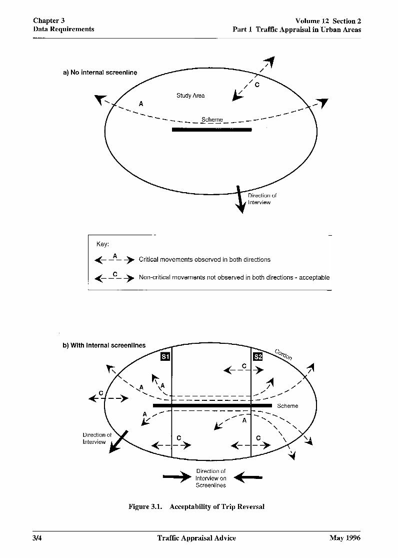
It is not advisable to derive peak period trip data for critical movements see section 3.2.5 in the non-interview direction by reversing interview-direction data from the other peak period.
I I
This means that the configuration of cordons and screenlines should enable critical movements to be observed in both directions (e.g. alternate cordons or screenlines could be surveyed in opposite directions - see Figure 3.1) _ In circumstances where this cannot be achieved, interviews may have to be carried out
in both directions (not necessarily on the same day) at some locations. The increase in reliability of the data must be balanced against the additional cost and disturbance involved in interviewing in both directions.
3.2.10 If parking information is to be included in a cordon survey (around a town centre, for example) it is desirable that such interviews are curried out in the ‘outbound’ direction (at leas0 to maximise the reliability of the parking locations given by respondents.
May 1996 Traffic Appraisal Advice 313
Chapter 3 Data Requirements
Volume 12 Section 2 Part 1 Traffk Appraisal in Urban Areas
a) No internal screenline
Key:
(- -*- + Critical movements observed in both directions
(- -‘- + Non-critical movements not observed in both directions - acceptable
With internal screenlines
\ Direction of Interview *A
Figure 3.1. Acceptability of Trip Reversal
Traffic Appraisal Advice May 1996

Volume 12 Section 2 Part 1 Traffic Appraisal in Urban Areas
Chapter 3 Data Requirements
3.2.11 Where motorways cross the study area, screenlines should be aligned with them and particular care taken with the screenline definitions. Since it is not usually possible to conduct interviews on any main carriageway and any busy off-slip road, motorway movements muy need to be interviewed by siting the surveys on on-slip rouds and adding a question about the exit used, or by using nearby locations and a ‘motorway use’ question, so that appropriate steps can be taken to deal with these movements when constructing trip matrices as set out in paragraph 4.3.15.
3.2.12 When a mixture of old and new data is to be used, it is desirable that, as far as possible, each screenline consists of only new or old (i.e. factored) sites, so that different levels of accuracy are not mixed in the same screenline.
3.2.13 Further discussion about the design of survey screenlines is included in Chapter 4, in the context of trip matrix construction.
3.2.14 In urban or congested areas there is often considerable scope for drivers to avoid roadside interview sites, and special care should be &ken with site selection and with the monitorirzg of alternative routes, for example, by the use of automatic traffic counts or by undertaking manual counts on the survey day and on another day. To minimise such problems, it is desirable to stop vehicles for as short a time as possible, by careful planning of site layouts and by limiting the number of questions to the minimum required to construct trip matrices. If necessary, delays can also be reduced by using self-completion (postcard) questionnaires that are returned by post, for part of the survey day. Postcard surveys can sometimes be located at traffic signals to further reduce delays to motorists.
3.2.15 Typical response rates wilh postcard surveys are of the order of 2540%, meaning that the number of questionnaires distributed should be at least 3 to 4 times the number of interviews that would have been carried out in a conventional survey. Goods vehicle drivers often have lower response rates, and consideration should be given to using direct interview methods for goods vehicles, even ifpostcards ure being used for other vehicle types. The generally low response rates associated with self-completion surveys can lead to biased results, andpostcard surveys should only be carried out as u lust resort, for the shortest possible duration, and where direct interviews would be impracticul or would cause unacceptible congestion,
3.2.16 The collection of origin to destination data at roadside interview sites is discussed in Sub-Section 6.4 of TAM which, in turn, refers to Advice Note TA 11/81.
Registration number surveys
3.2.17 Registration number surveys have several disadvantages over interview surveys: the trip data lack details of travel purpose and of the ultimate origin or destination of the trip; and data processing (registration number matching) can also be complicated, time consuming and subject to bias. The advantages are the absence of intrusion and a lower unit cost of observation. Reg&ration number szlrveys cun sometimes be lrsed for limited validation of or&in to destination data in s~nall or closed systems, where interview surveys would be dtJEcult to carry out. For example, they may be used to check movements using ‘rat runs’ or to provide entry to exit data for motorways, or smaller junction or road improvement schemes. They may also be used to establish overall journey times through part of the study area. The use of regktration number surveys is not recommended, however, if there ti u large number of tri)s terminating within the szlrvey area.
3.2,18 Guidance on carrying out registration number surveys, where these are required, is given in Sub-Section 6.7 of TAM.
May 1996 Traffic Appraisal Advice 31.5
Chapter 3 Data Requirements
Volume 12 Section 2 Part 1 Traffic Appraisal in Urban Areas
Count Data
3.2.19 Traffic count data are used to calculate the sample factors to be applied to roadside interview data, to adjust origin to destination data to a common time base, and to validate the traffic flows output by the base year assignment model. When updating trip matrix data, counts can be used to derive the factors to be applied to various parts of the matrix, by vehicle type. Procedures for collecting automatic and classified count data are outlined in Sub-Sections 6.5 and 6.6 of TAM. Count data are an important element in calibration and validation. TAM gives guidance on estimating their accuracy, including the effects of factoring from one situation to another. Counts with 95% CI’s wider than +. 15% should not be used in calibration or validation.
3.2.20 Automatic traffic counts are usually the cheapest, simplest and most accurate and reliable form of count data available, although their use at locations with regular queues should be avoided. They are used for all the purposes mentioned above and, in addition, can be used to monitor traffic flows during the study and to provide information about the relationship between survey day traffic and longer term flow levels. Automatic counts can also be used to provide information about local 12-, 16- and 24-hour flow ratios, and daily and seasonal traffic variations, all of which are required to estimate average daily traffic flows from shorter period data.
3.2.21
AU roadside interview sites should bc included in count programmes for at least 2 weeks, but only a selection of representative sites need be used for the measurement of longer term factors such as seasonal variation. At least one automatic traffic counter should be installed on the key route(s) relieved by the scheme and maintained in continuous use throughout the scheme preparation period.
Manual classified counts are required to break down traffic flows by vehicle type. This information is particularly important in an urban area, where the mixture of vehicle types may vary significantly by direction as well as at different times of day. Classified counts are reqzcired at every roadside interview site, and on minor parallel roads not included in the interview programme, to expand the interview sample to the total traffic flow in the corridor as a whole (see Paragraph 4.3.13). Coz~zts shozzbi be carried ant in both directions on the survey day, even ifinterviewing is only in one direction, and shouzif extend over all model periods. If azctomatic cozznts indicate that traJiccflows at a roadside interview site were influenced by the presence of the interview survey, further manzuzl classzj’ied cozcnts shozzW be made on a different day. If necessary, these alternative counts can then be used to expand the interview data to a more representative traffic flow. The vehicle classification used should correspond with that used in the interview survey itself, and this in turn should be compatible with the vehicle types represented in the traffic model.
3.2.22 Tumin,e counts at road junctions are required for the calibration and validation of junctions in a congested assignment model. Tmxing counts should be carried out at allj*zuzctz*ons within the model area that are likely to have a sign@ant impact on journey times or delays and at jzznctions that are particzzlarly significant in route choice (i.e. locations where alternative rozztes for critical movements may merge/diverge). In urban areas, there will often be a need to collect more turning count data than for an inter-urban model, because of the greater number of junctions that generally need to be validated.
3.2.23 Turning counts are carried out in the same manner as manual classified counts on links, except that more enumerators are generally required. They mzzst cover the whole of eachpeakperiod, but need only cover representative parts of other time periods. The vehicle classification used may be simpler than the one used for link surveys, provided that it is again compatible with the model classification.
316 Traffic Appraisal Advice May 1996
Volume 12 Section 2 Part 1 Traffic Appraisal in Urban Areas
Chapter 3 Data Requirements
Network Data
3.2.24 The network data required to calibrate and validate the traffic model includes measurements of journey times, and queue lengths and/or delays at road junctions. Other data describing the geometric characteristics of the network, and its operational characteristics at different times of day, will also be required. General guidance on the measurement of journey times, queue lengths and delays is given in Sub-Section 6.8 of TAM.
For the appraisal of urban trunk road schemes, journey time measurements should cover all critical movements (see Paragraph 3.2.5) through the study area, and queue and/or delay data should be collected at all significant junctions used by those critical movements.
3.2.25 Journey time measurements are an essential part of assignment model validation for most urban traffic appraisals, since the majority of scheme benefits tend to be related to journey time savings. Comparison of observed and modelled journey times gives a measure of the appropriateness of the speed-flow relationships for a capacity restrained assignment, as well as the junction delay calculations for a congested assignment model. Journey time surveys may also be used to identify junctions that need to be modelled in detail.
3.2.26 Journey time information may be collected using either the ‘moving observer’ method (in which a car travels through the network on a series of fixed routes, and at the average speed of other traffic) or by using registration number surveys. As already mentioned, the latter should only be considered for a closed system, such as motorways, where the number of intermediate stops is low. Moving observer surveys can give more information (eg about the cause of delays). However, drivers carrying out moving observer surveys cannot be instructed to exceed the speed limit, which makes the technique less suitable where average speeds exceed the speed limit.
3.2.27 Joluney time rorctes for movilrg observer surveys should be defined so that euch contains relatively homogeneorrs traflc conditions (e.g. urban, suburban or rural). In general, routes should not be excessively LOJ~ (greater than about 15 Km) or excessively short (less thun about 3 Km), allhough the lengths will depend on the nature of the critical movements. In urban areas, the turning m.ovements through which the route passes should represent a realistic series of turning movemenfs likeb to be used by the majority of crifical movements.
3.2.28 During the survey, the total travel time shouti be recorded separately for each road section between muJ*orjurzch’o?zs and, because junction delays form an important part of travel lime in urban areas, a separate note should be made of the delay time at each junction. Ideally, delay should be assumed to start once instantaneous speed falls below a chosen speed, say 15 kph (IO mph). Journey time n171s, in both directiorti and in euch model time period, should be made over u period of several days. Variations in travel times during peak periods should be taken into account by staggering start times, to represent fairly conditions over the time period as a whole.
May 1996 Traffic Appraisal Advice 317
Chapter 3 Data Requirements
Volume 12 Section 2 Part 1 Traffk Appraisal in Urban Areas
3.2.29 Detailed guidance on the number of journey time runs required to achieve a given level of accuracy is given in Sub-Section 5.10 of the COBA manual. These give the acceptable 95% confidence level of accuracy as ~10%. over a route as a whole. Four initzizljoumey time runs (each on a diJ%rent day) should be made for each route, direction and model time period, and the results used to assess the variability of journey times in each case. Further runs mrrst then be made for those routes, directions or timeperiods in which the vahbility falls outside this acceptable range. In urban areas, where journey times can sometimes be erratic, this may lead to a large number of runs being required. If a satisfactory level of accuracy has not been achieved after 12 runs, the results should be accepted, and a special note made in the survey documentation.
Queue Length and Delay Measurements
3.2.30 Queue length and delay measurements provide information for the calibration of congested assignment models. These quantities are the most detailed outputs of the model and are therefore the best measure of its ability to predict the effects of flows on junction delays. Queue length measurements arc more common, since they are easier to measure, although delays are of greater importance in the economic appraisal. Both are somewhat subjective to the extent that they depend on the judgement of individual 0
observers as to whether traffic is queuing or just moving slowly. Queues and delays can vary appreciably from day to day, and so data should be collected over several days.
3.2.31 Queue (or delay) information should be collected at all junctions in the model area that are likely to have a significant impact on journey times or delays _ As with turning count measurements (Paragraph 3.2.22), the survey should cover the whole of each peak period, together with representative parts of other modelled periods. Stationary observers (at road junctions) are normally used for this purpose, but information from moving observer journey time surveys can supplement these delay measurements. The queue length at each junction approach lane should genera& be recorded at regular (say, S-minute) intervals during each of the peak periods. However, at sign&tied junctions both the maximum and minimum queue lengths in each signal cycle should be recorded. A note should also be made of the extent and duration of any interaction between adjacent junctions (‘blocking back’), as well as any unexpected operational characteristics of the junctions.
Other Geometric and Operational Data
3.2.32 Other geometric and operational data will be needed to calibrate the assignment model. In simple situations, where link based modelling methods are adequate, only link data are generally required. When a congested assignment model is to be calibrated, more detailed information about the layout and operation of junctions will be needed to allow the network to be described in a realistic way.
3.2.33 Geometric information may be obtained from maps and large scale plans, from any existing inventories held by the highway authority, and/or by field measurements. For road links this will include the length and average width of each section; at junctions it will include the number and width of approach lanes, and other relevant aspects of junction layout. Operational information, such as signal timings, banned turns or one-way streets, may be available from local authority records, but in many cases it will be necessary to observe these directly. Further information about the preparation of highway network descriptions is included in Chapter 4.
3/a Traffic Appraisal Advice May 1996
Volume 12 Section 2 Part 1 Traffic Appraisal in Urban Areas
Chapter 3 Data Requirements
Parking Supply Data
3.2.34 Parking supply data will be required if the traffic model is to include the detailed representation of a town centre, or other area where the supply of parking spaces is restricted. This information is used to check that the estimated number of trips starting or ending in the area, in each time period, is consistent with the supply of public and private parking spaces. The numbers and usage of privately owned parking spaces can be particularly difficult to survey. Also, if the trip ends are related to the driver’s ultimate origin or destination, parking supply data may be required to re-allocate trips to the associated parking zone(s), prior to carrying out the highway assignment.
3.2.35 Parking supply information can usually be provided from local authority sources, but where this is not available, appropriate surveys will need to be arranged. It is important that parking supply data include all types of parking, i.e. on-street, public and private off-street (both residential and non-residential). Data on the supply and usage of private non-residential parking spaces may be important, but are often difficult to collect.
Public Transport Data
3.2.36 Public transport data, relating to the number and frequency of buses, will be required for parts of the study area where they represent a significant proportion of the traffic flow, or where the proposed road scheme is expected to have a significant impact on the route@ of bus services. This is readily available from timetables and other similar sources.
3 -2.37 In those cases where a comprehensive transport model is required for the adequate appraisal of a particular trunk road scheme, more comprehensive information about the pattern of public transport usage will also be required. This will usually involve surveys to collect the necessary origin to destination and count data (vehicles and occupancy) _
Planning Data
3.2.38 Planning data, giving details of present and future land use and socio-economic characteristics of each model zone, will be required if a local trip end model is to be used as part of the traffic forecasting procedures, or if National Trip End Model output at the local authority District level is to be broken down into finer areas. Suitable data can usually be obtained from local planning authority sources, although sufficient time should be allowed for what is often a lengthy activity. It will be particularly necessary to hizise close0 with Local planning authoriries to determine the likelihood, location and timing of any future new developmenti.
l May 1996 Traffk Appraisal Advice 319
Chapter 3 Volume 12 Section 2 Data Requircmcnts Part 1 Traffw Appraisal in Urban Areas
3.3
3.3.1
3.3.2
3.3.3
3.3.4
3.3.5
3.3.6
USE OF EXISTING DATA
General rules about the re-use of data were given earlier, in Sub-Section 2.10. Pressures of time and cost often encourage the use of old data, but this cannot be justified if the data are unsuitable for the current purpose.
The likely accuracy and relevance of old data must be established before they can be used in a new study. It is therefore essential that any such da&a are well documented. Inherent accuracy is a question of the sample size of the original data (or, in the case of count data, the type of data) and any calculations that may be applied to bring it to the base of the traffic model. In addition, data may no longer be appropriate if circumstances have changed significantly; for example, if substantial changes in land use or network infrastructure have occurred that change the previously observed pattern of travel.
Origin to destination data are frequently re-used, as they are expensive and difficult to collect. The various methods available for re-use of such data are discussed further in Chapter 4, under the heading ‘Matrix Updating Methods’ _ Count data for this purpose may already exist for many sites within the study area (from local authority or overseeing Departments’ sources) in which case only a limited number of additional counts may be necessary (but see also Paragraph 3.2.19).
Journey time, queue length and delay data cannot be updated reltibly. If such data are to be re-used, samples of the data should be checked against new measurements to ven;fr that traflc conditions have remained the same since the otiginal measurements were made. A check should also be made to ensure that other factors, such as junction layout and signal timings have remained the same. In general, such data should be re-used with extreme care and only in exceptional circumstances.
If a traffic model, such as a regional or county model, already exists for the scheme area, it may be possible to re-use all or part of it for the new appraisal. The trip matrices from such models may be suitable for re-use, assuming that the zoning systems are compatible or can be adapted. However, any ex&ing tr@ matrices that are used in the new model must be re-validated against recent independent data, usually traflc counts. Network and assignment aspects often need more substantial preparation work to satisfy the objectives of the new appraisal. The existing network description can sometimes be taken as the starting point when preparing a network for the new traffic model, by adding junction details, for example. If network itlformation is adapted from a previous study, it must be thoroughly checked for coding and other errors, and for compah*bility and consistency with the requirements of the new model.
The use of existing model information to construct new trip matrices is discussed in greater detail in Chapter 4.
3/10 Traffic Appraisal Advice May 1996
Volume 12 Section 2 Part 1 Traffic Appraisal in Urban Areas
Chapter 3 Data Requirements
a 3.4
3.4.1
3.4.2
DATA PROCESSING AND ANALYSIS
Before the traffic model can be developed, any data collected must undergo basic processing. Data entry must be undertaken and coding and editing procedures must be defined and performed.
The most significant element in the coding of origin to destination data is the allocation of zone codes. For simple studies it may be possible to convert the addresses given in interviews directly to zone codes. However, as this limits the usefulness of the data for other studies with different zoning systems, it is recommended thut a standard locational reference, such as a postcode or Ordnance Survey gTicl reference (OSGRA is used. This automates the allocation of zone numbers as well as overcoming this problem. To retain maximum flexibility, the postcode or OSGR should be kept on the processed trip record, in addition to the zone code. If other types of address location system are used, they should be treated in the same way as postcodes or OSGRs. If necessary, special codes (referred to as ‘dump codes’) should be used to represent non-postal or partial addresses. Any txips associated with these addresses can then be re-allocated to actual zones, immediately prior to matrix construction.
Sensible range and logic checks, including direction checks, must also be carried out on interview da& prior to its acceptance for use in a traffic appraisal. The checks carried out and the number of records amended or rejected at each stage must be reported, as an indication of the quality of the data.
3.5 REPORTING REQUIREMENTS
3.5.1 It is important that the results of all traffic surveys associated with a scheme appraisal are properly documented, stored and made accessible for use in future traffic models. A Survey Report covering all aspects of data collection must be prepared for this purpose. This will form an important component of the traffic study database documentation and will provide reference material for any subsequent users of the data. The items that should be included in the report, and the form of their presentation, are outlined more fully in Appendix A.
May 1996 Traffk Appraisal Advice 3/11
Volume 12 Section 2 Part 1 Traffx Appraisal in Urban Areas
Chapter 4 Traffic Model Development
4 Traffic Model Development
4.1 GENERAL
4,1.1 An overview of the issues involved in traffic model development has been given in Chapter 2. Guidance has also been given in Chapter 3 regarding the input data that are likely to be required. The objective of this chapter is to examine in detail the methods involved in developing a traffic model for urban trunk road appraisal. Initially, this model will be required to reproduce base year traffic conditions; subsequently, it will form a base from which future traffic levels can be projected, and the impact of the proposed scheme(s) investigated. It is therefore important that it can be shown to give a realistic representation of present traffic conditions, and that it has the facilities required to reflect perhaps extensive changes that might occur in the future. At the same time, the methods used should be as simple and cost-effective as possible, consistent with achieving these objectives.
4.1.2 The steps involved in developing a traffic model for the base year include:
Specification
0 defining the most appropriate model structure for appraisal of the scheme under consideration;
0 defining the area to be modelled, and designing an appropriate zoning system and network description;
0 if required, setting out the proposed methodology in an Inception Report;
Data Collection
0 reviewing the existing and new data that will be required to construct the model,
0 carrying out the appropriate surveys and preparing the data for use in the model;
Model Calibration and Validation
0 constructing and validating a base year trip matrix;
0 constructing and validating a base year network;
0 calibrating and validating an assignment model;
Reporting
0 preparing a local model validation report; and
0 if required, technical working notes.
Further details of these steps are given in the remainder of this chapter.
May 1996 Traffic Appraisal Advice 4/l

Chapter 4 Trtic Model Development
Volume 12 Section 2 Part 1 Traffic Appraisal in Urban Areas
Model Structure
4.1.3 The types of model structure that are likely to be appropriate for traffic appraisal in an urban area have already been outlined in Sub-Section 2.3. These range from simple models of individual junctions to more sophisticated network-based traffic models that cover the full range of characteristics associated with traffic in urban areas.
It is important to decide on the structure of the model at an early stage in the traffic appraisal process. As already stated, the aim must be to specify the form of model required to deal with the features of the study under consideration without introducing unnecessary complexity.
4.1.4 One of the factors to be considered when deciding the form of a traffic model, is the way in which the network is to be coded and, more particularly, the type of assignment model that is required. For urban schemes, some or all of the following assignment model capabilities are likely to be relevant:
the ability to model the variation of traffic flows within a given time period;
realistic representation of special features of urban road networks (one-way systems, banned turns, etc.);
an assignment algorithm that recognises the inter-relationship between traffic flows, capacities and delays (speeds);
realistic calculation of downstream flows, where capacity is restricted at a particular bottleneck (whether at a road junction or elsewhere) ;
estimation of capacities, queue lengths and delays at road junctions (with values for individual turning movement being estimated separately, for maximum realism);
the ability to distinguish between junction types (e.g. allowing U-turns at roundabouts, but not at traffic signals or priority junctions);
realistic treatment of ‘blocking back’, where queues at a junction impinge directly on the operation of upstream junctions;
separate treatment of the different vehicle types represented in the model, including road-based public transport vehicles, if appropriate; and
facilities to interface with public transport modelling software, if appropriate.
However, only those capabilities that are relevant to a given study should be included. Assignment techniques are discussed in greater detail later in this chapter.
412 Traffic Appraisal Advice May 1996
Volume 12 Section 2 Part 1 Traffic Appraisal in Urban Areas
Chapter 4 Traffic Model Development
a 4.1.5 Whichever type of model is selected, one or more trip matrices will need to be prepared, either from
survey data or from other sources.
In urban and peri-urban areas, traffic models should normally be sub-divided into separate time periods (e.g. AM peak, PM peak and inter-peak), each with its own distinct travel characteristics, and separate trip matrices will be required for each of these time periods.
In addition, it will UWU~~ be necessary to construct tn) matrices for separate journey pqoses and/or vehicle types, to reflect their different distribution, mode sensitivity and growth patterns. The individual trip purpose matrices will normally be combined, however, prior to assignment. Separate assignment of these trip matrices can only be justified if the travellers concerned are believed to exhibit different behaviour patterns, or if there is a need to identify them separately in the final traffic flow. Some assignment packages allow the level of demand to vary between ‘time slices’ within the time period covered by the trip matrix. The use of ‘time slices’ is discussed later in this Chapter and in Appendix D.
4.1.6 Models are usually required to represent a typical period of the year, and should thus avoid modelling the absolute worst conditions that may arise. Further information about the methods used to construct trip matrices for the base year is given later in this chapter. Techniques for forecasting future trip matrices are discussed in Chapter 5.
Validation Principles
4.1.7 The role of model validation has been mentioned briefly in Chapter 2, and more detailed guidance is given in Chapter 11 of TAM. The principles involved are similar for both inter-urban and urban schemes.
4.1. .8 The software used to operate the model must be capable of supporting the model structure chosen for the appraisal of the scheme under consideration. The most critical aspects will usually relate to the type of assignment model that is deemed to be necessary, and which of the features listed in Paragraph 4.1.4 are required. The assignment model software must be capable of giving traffic flows and speeds on all links in the scheme area (and turning flows and delays at selected junctions, if required). The ability to accumulate travel times along predefined routes is also desirable to facilitate the comparison with journey time data. Finally, the software package used should provide a convenient means of analysing the origins and destinations of trips assigned to a given network link (‘select link analysis’), in a way that is compatible with the main assignment procedure.
Each stage of base year model development should be validated against independent data, so that any weaknesses in the model can be properly understood and remedial action identified.
I I
Independent counts used in validation must be on different links from those used in calibration, preferably with at least a road junction or zone loading point in between. Any remedial action required should be undertaken before proceeding to the next step. The question of model validation is a recurring theme in the discussion that follows in the remainder of this chapter.
Software Requirements
May 1996 Traffic Appraisal Advice 413
Chapter 4 Traffic Model Development
Volume 12 Section 2 Part 1 Traffic Appraisal in Urban Areas
4.1.9 Base year trip matrices can usually be developed using any software that contains the appropriate procedures _ These include:
0 tabulation of survey data to form origin to destination matrices;
0 merging origin to destination data from various sources (screenlines);
0 matrix arithmetic (addition, subtraction, simple multiplication (factoring), division and matrix multiplication);
0 matrix transposition;
0 the estimation of unobserved movements from observed movements (‘partial matrix’ techniques); and
0 matrix estimation or adjustment using count data.
4.1.10 Matrix adjustment procedures such as matrix estimation by maximum entropy (ME2), that rely on network and traffic assignment characteristics for their operation, should use the same network descriptions and assignment methods as the main model. This usually requires that they are taken from the same software package as that model. (see Paragraph 4.3.28 ff.)
4.1.1 1 Procedures associated with the merging of origin to destination data should take account of the respective accuracies of the different data sources (as described in Sub-Section 8.7 of TAM). They should also be able to estimate the statistical errors associated with the merged data. At present, the only readily available software that calculates accuracies and takes them into account in matrix manipulation are the Department of Transport’s MATVAL package and EFUCA program (see Paragraph 2.11.3). Trip matrices produced by these programs can usually be converted to the format of other packages for further processing, if required.
4.1.12 The full significance of some of the above software requirements will be made clearer in the remainder of this chapter. The software requirements associated with traffic forecasting are described further in Chapter 5.
Study Area and Zoning System
4.1.13 The definition of the area to be covered, and the level of detail requird for each part of the model area, are important considerations in the design of a traffic model. The issues involved in identifying a scheme study area were referred to in Sub-Section 2.4, and can also be found in Sub-Section 3.1 of TAM. There will always be a degree of interdependence between the definitions of tbe study area/zoning system and the network, such that one should not be defined without reference to the other.
In general, the scheme study area should be as small as is consistent with the requirements of the economic appraisal, but large enough to reflect likely reassignment and induced responses to congestion and to the scheme in the future.
Trafic Appraisal Advice May 1996

Volume 12 Section 2 Part 1 Traffic Appraisal in Urban Areas
Chapter 4 Traffic Model Development
4.1.14 The model area is usually divided into an ‘internal’ (or ‘study’) area and an ‘external’ area, ideally with the boundary between the two being marked by an external cordon of roadside interview sites. The boundary between the ‘internal’ and ‘externul’ model areas should be located so as to delineate the areu of injluence of the scheme being apprahed, in terms of significant tr@ic flow changes (as advocated in Chapter 3 of TAM). Existing models are sometimes designed for use in appraising a number of road schemes within a given local authority area, with the external cordon being located at an administrative (e.g. county) or other convenient boundary. In such cases, the original boundary between the ‘internal’ and ‘external’ model areas may need to be relocated to suit the requirements of the individual scheme being appraised (if this is possible with the data that are available).
4.1.15 If external trips are loaded onto the network at the cordon crossing points, then information on the external end of the trip will be lost. This can cause problems at later stages: if a gravity model is to be used to infill a partially observed matrix (see Paragraph 4.3.18 ff) ; during the development of traffic growth factors; and if induced traffic is a key feature of the subsequent assessment. lhe alternative of defining an ‘external’ network can allow reassignments in the ‘external’ area, and is preferable provided the change in vehicle hours and miles in the external area is monitored and taken into account in the economic analysis stage.
4.1.16 In the ‘internal’ area, all traffic movements generally need to be included, so that the model can provide realistic estimates of the travel characteristics that are likely to prevail in a given situation. In the ‘external’ area, modelling methods are often simplified, with only the traffic flow associated with the study area itself being included. Consequently, capacity restraint, detailed junction modelling and traffic flow validation are not usually relevant in this part of the model area.
4.1.17 The zoning system is also an important part of the traffic model, since it provides the basis for defining the origins and destinations of trips. Guidance on the design of a local model zoning system is given in Sub-Section 3.2 of TAM, and much of this holds good for urban as well as inter-urban schemes. The following paragraphs emphasise and expand those issues that are most relevant to the construction of zoning systems in urban areas.
4.1.18 In the ‘internal’ area. zone boundaries should seek to take account of:
0 natural barriers (rivers, railways, motorways or other major roads);
0 areas of similar land use that have clearly identifiable and unambiguous points of access onto the road network included in the model;
0 existing zone boundaries, where an existing model is being used as the basis for the new model;
0 administrative and planning data boundaries (wards, parishes, Census enumeration districts);
0 the location of the main parking areas, where town centres are included in the model; and
0 the need for internal screenlines for trip matrix validation.
4.1.19 The objective of the ‘external’ model is to enable traffic flows at the study area boundary to be estimated within acceptable levels of accuracy, and the zoning system in the ‘external’ area should reflect this objective. This will usually involve an appreciation of the catchment areas of the main roads crossing the study area boundary. Zone boundaries in the ‘external’ model area should follow local authority boundaries wherever possible.
May 1996 Traffk Appraisal Advice 415
Chapter 4 Traffic Model Development
Volume 12 Section 2 Part 1 Traffic Appraisal in Urban Areas
Zone Size
4.1.20 The size of traflc zones B a critical factor in determining the realism and accuracy of the tra@c model. If zones are too large, the model will be unable to estimate traffic flows to the required I.evel of precision, however good the quality of the trip matrix data. On the other hand, if the zones are too small, the sample sizes in the cells of the matrix will be small also, affecting the accuracy of the trip and flow estimates. Typically zones need to be large enough to generate 200 trips per hour across the screenlines or cordons. Some will need to be smaller than this, to model their loading points sufficiently accurately. Beyond that, any major increase in the number of zones with fewer trips is likely to increase the complexity of the model without adding significantly to real model accuracy. Small zones should be concentrated in the key parts of the study area. As a guide, the total number of zones required for an urban traffic model for the appraisal of a road scheme is likely to be between 50 and 200. A smaller number may be appropriate when modelling the impact of simple junction improvement schemes.
4.1.21 In this context, it should also be noted that intra-zonal trips (i.e. those taking place entirely within the same zone) are not assigned to the model network. If zones are too large, this may lead to a significant underestimation of traffic flows, both on links and at junctions, and this in turn could seriously distort the pattern of flows and delays given by the assignment model. This is a particular problem in urban traffic models that use capacity restraint assignment techniques. Similar distortions, particularly in the modelling of junction turning movements, can also occur if zone sizes are not compatible with the level of network detail included in the model. A more detailed explanation of this issue is given in Paragraph 4.2.6.
4.2 NETWORK DESCRIPTION
4.2.1 Network descriptions in urban areas will often need to include both link and junction details. Links are usually described in terms of:
0 the reference numbers at the ends of the link (i.e. ‘nodes’);
0 the link length;
0 the base year travel speed on the link (during the time period being modelled) ;
0 the speed-flow relationship (if any) appropriate for the link;
0 the link capacity, if not defined by the speed-flow relationship, or junction details;
0 whether the link operates in both directions or in one direction only; and
0 any restrictions to particular vehicle types using the link.
In urban areas it may sometimes be necessary to consider the impact of traffic management measures such as bus lanes, traffic calming, ‘Red Routes’, parking controls and cycleways, on the capacity and operating speed of individual network links. The way in which the above information is input to the model may vary slightly according to the software package that is being used.
Traffic Appraisal Advice May 1996
Volume 12 Section 2 Part 1 Traffic Appraisal in Urban Areas
Chapter 4 Traffic Model Development
-
4.2.2 The way in which junctions are described also varies between different modelling packages. The usual requirements are:
0 the junction type (traffic signals, roundabouts, priority) ;
0 the number of approach arms, and their order (in terms of entry link references);
0 the number and width of traffic lanes on each junction approach, and the lane discipline adopted (including prohibited turns);
0 any additional data required to describe the operational characteristics of the junction (e.g. saturation flows, signal timings and phasing, turning radii and gap acceptance characteristics).
The most useful packages are those that provide maximum flexibility for coding unusual junction layouts, and that estimate junction capacities from geometric inputs while still allowing these capacity values to be over-ridden in special circumstances _ Some packages allow traffic signal times to be calculated directly from the assigned traffic flows but, as will be seen later, widespread use of this facility can lead to instability within the assignment model. For this reason, it is preferable to specify fixed timings for all traffic signals included in the base year network (even though this may mean coding different times for each model time period and/or time slice) and these should reflect the existing settings.
4.2.3 The level of network detail required in the ‘internal’ model area will be greater than in the ‘external’ area. In the ‘internal’ area, it will be necessary to include all main roads, as well as those secondary routes, or roads in residential areas, (including ‘rat-runs’) that are likely to carry critical traffic movements, either in the base year or in future years. Modelling this traffic may present some technical difficulties, but it is most desirable that the effectiveness of the scheme in attracting it back to the main road network, is accurately assessed. Local highway authorities will normally be aware of the common ‘rat-runs’, but some independent assessment may also be required. In the absence of count data, accident plots may also give an indication of rat-running traffic.
4.2.4 Capacity restraint should usually be applied throughout the ‘internal’ model area. Separate junction modelling will also be required in those parts of the ‘internal’ area where junction capacities have a significant impact on drivers’ route choice, and where delays are not adequately included in the speed-flow relationships applied to network links. Care must be taken to specif real&&c capacities throughout the ‘internal’ model area and in the choice of turning movements for which it is necessary to specl;fy indivtiuul turn capacities. In selecting an internal area, the need for continuity and consistency of procedures such as ‘flow metering’ and ‘blocking back’ can be important. Some software packages require continuity of modelled junctions for such procedures and without consistency analysts can inadvertently encourage unrealistic routes avoiding flow metered routes.
4.2.5 In the ‘external’ model area, the network description will need to cover all routes necessary to feed traffic to the boundary of the ‘internal’ area in a realistic way (i.e. with realistic distances and speeds). Again, care must be taken not to encourage unrealistic reussignments to routes that could avoti the ‘internal’ area, especially if fixed speeds are specified on external network links and no capacity restraint is applied, as is normally the case.
4.2.6 In most packages, special links (usually referred to as ‘zone connectors’) are used to load traffic onto the model network, although some allow other forms of zone loading. The position of these connectors is often a critical fact,or in achieving realistic results from the assignment model. In the ‘internal’ model area, they must be located as realistically as possible, and in particular must not be connected directly into modelled junctions, unless a specific arm exists to accommodate that movement. Reference has already
May 1996 Traffic Appraisal Advice 417
Chapter 4 Traffic Model Development
Volume 12 Section 2 Part 1 Traffic Appraisal in Urban Areas
been made to the relationship between the realism of zone connectors and the size of zones in the ‘internal’ model area. If zones are significantly larger than implied by the detail of the network, it will often be impossible to locate zone connectors realistically. This may lead to distorted traffic flows on nearby links, and turning movements at nearby junctions, which may themselves distort traffic patterns elsewhere in the network. In urban areas in particular, zones should be small enough to avoid this type of problem.
Parking
4.2.7 me need for and the method of handling parking choice in any town centres etc. mmt be decided at an ear& stage of model development, since it will influence the zoning system, the way that origin to destination data are collected, the network description and the results of any multi-modal modelling. Three techniques are available: the first defines vehicle origins and destinations in terms of parking locations alone; the second involves the relocation of person origins or destinations to the most likely parking areas by adjusting the trip matrices, and the third defines a series of ‘walk or park-and-ride links’ between parking locations and ultimate destinations.
4.2.8 In most trunk road appraisals that are the subject of this guidance, the detailed modelling of parking is not usually a crucial issue. Where it is, it should be noted that the first method breaks the direct relationship between land use and traffic generation, but may be the most appropriate method where simple factoring is being used to forecast future traffic levels. Where matrix adjustment is used in connection with the second method, subjective judgements are required, particularly about the way drivers will react to a limited number of parking spaces as demand increases, or to park-and-ride schemes. Although the method involving ‘walk links’ gives flexibility within the model itself for drivers to choose alternative car parks, according to the direction by which they approach the town centre, care must be taken with this method to control the proportions who can choose the walk or park and ride option, to reflect that not all drivers will be prepared to walk far and to recognise car park capacities.
Network Checking
4.2.9 Most network modelling packages contain procedures for checking the integrity of the network description. Further checks should be carried out by:
0 checking the routes through the network, produced by a standard path building algorithm; and a
0 accumulating travel times (and distances) along the journey time routes, from the network description, and comparing these with the travel times observed during the journey time surveys.
Care should be taken to ensure that the calculations and compations involved in these initial checks are meaning$J, especially as delays at explicitly modelled junctions will not have been calculated at this stage. Some network and assignment model packages allow initial estimates of junction delays to be included in the network description, and this facility should be used if available. Further checks should be carried out at a later stage (see Paragraph 4.4.32).
Traffic Appraisal Advice May 1996
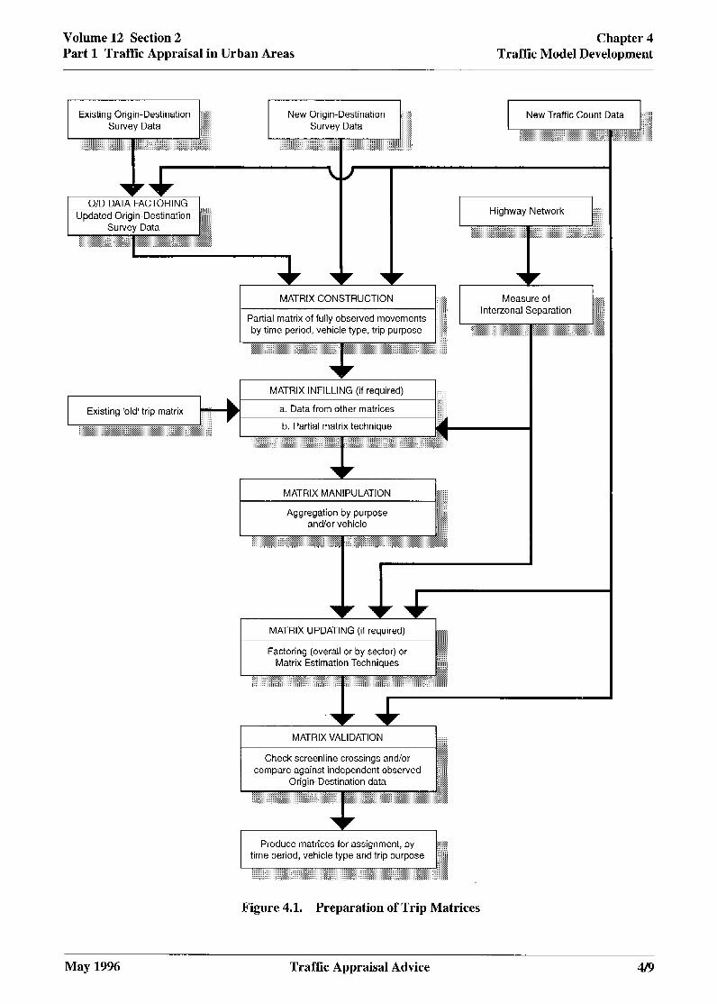
Volume 12 Section 2 Part 1 Traffic Appraisal in Urban Areas
Chapter 4 Traffic Model Development
Existing Origin-Destination :i:.!:
l ~~~
MATRIX INFILLING (if required)
a. Data from other matrices
O/D DATA FACTORING Updated Origin-Destination ‘/ii Highway Network ““:
::::::
MATRIX CONSTRUCTION ..,,,, :://// :i;;;; ::::::
Partial matrix of fully observed movements :::: : iii;;;.
by time period, vehicle type, trip purpose ::‘:“, . iiii.‘ii
Measure of / ./:
lnterzonal Separation ;$ ;;;;‘; ,, ,,:,:/,:
gr::::, I > /,,,,,,,,,, ::::::::::~ ,:, >: :.,.:::, :< /,,,,,.,..,,,,,,,, :::::: 2 :‘:,:, ::::::::, I, ..,. (‘: : :v1::::::,,:,,,,,:,’ /<// :’ ,,,,,,,,,,,,,,,,. :I:, ,.,,,, ,,,,.., .::,, : ,,:,,:, ::::::
MATRIX MANIPULATION ;;;;ii’ ;;;;ii<
MATRIX UPDATING (if required) :::::: :::::: :::::: ::::::
Factoring (overall or by sector) or ,‘!‘j’ Matrix Estimation Techniques I:);;;;
:““’ iiiiiiii:iiiiiiiiiiii:;li:ii’iizs!i-ii-’~,~~~:~~~ iiiiiiii‘::::::::i::: i.,!::.‘:::::::::l.i:iiir:i:::::::
MATRIX VALIDATION :: :F’
Check screenline crossings and/or :% compare against independent observed
ij:;
Origin-Destination data :i:i’i / ;:;$l; ;;;>u I
.y.., .::..A::::<:~~” ,.. ,,,,, :, ,,,,,,,,,,, ,, ,:,,:c;j/,, :,,, :,::,i:l‘::l:i”::,: :: .q,, :,,::,:,,,: ////,/, :ii:$ ::::::::::::::::::,:::::::: /:I;/ ,:i,::::~I:I..:::::::::::::~~~.,,~~::::’:,: ::, :>,:::: ::::::::::::: :,:,: .:.::::::::::::::::::::::::::: <::::
Figure 4.1. Preparation of Trip Matrices
May 1996 Traffic Appraisal Advice
Chapter 4 Traffic Model Development
Volume 12 Section 2 Part 1 Traffic Appraisal in Urban Areas
4.3
4.3.1
BASE YEAR TRIP MATRICES
Base year trip matrices are usually assembled using the following sequence of procedures (see Figure 4.1) :
0 O/D data factoring is the process by which old origin to destination data is scaled, preferably to new traffic counts at the old roadside interview sites or screenlines;
0 matrix construction is the process in which origin to destination data are used to calculate the observed movements of a trip matrix;
0 matrix infilling relates to the estimation of unobserved trip movements, either by using parts of another matrix, or by the use of a model;
0 matrix manipulation involves the combination of observed and infilled parts of a trip matrix, and other matrix manipulations required to obtain origin to destination matrices for assignment; and
0 matrix updating uses factors or count data to revise a matrix. a
4.3.2 There is an important difference between these techniques. Matrix construction and infilling can be carried out separately for different trip purposes and/or vehicle types, but matrix updating based on count data can only be applied to vehicle types.
4.3.3 As noted in Paragraph 4.1.5, the requirement to develop separate models for different parts of the day means that separate trip matrices must be assembled for each model time period. Two main methods of deriving trip matrices for individual time periods can be identified:
0 constructing matrices directly from the origin to destination data relating to the specific period;
0 constructing matrices by combining specified proportions of the ah-day (12 or 16-hour) Production - Attraction matrices for each trip purpose.
It is recommended that trip matrices for individual time periods are constructed directly from origin to destination data, so that the characteristics of each time period are represented as realistically as possible.
Model periods should be as long as possible, the whole of each peak period should be included (not just the peak hour), and the inter-peak should extend from the end of the AM peak to the start of the PM peak.
The first part of the recommendation does not necessarily apply to vehicle and purpose categories with very small numbers of trips (e.g. HGV or minor purposes). These are usually best handled by factoring the all-day matrices.
The second part of the recommendation arises as the collection of a single hour’s data is likely to be more subject to day by day variability than longer period data. Also there is growing evidence that in congested areas drivers have responded to the congestion they face and some of the longer distance drivers have either actively or passively retimed their journey to avoid the worst of the congestion. The use of single hour data can underestimate such longer distance trips and hence produce biased economic assessments. Its use in modelling would also present problems in any modelling of their return to the peak as a result of a scheme or of further peak spreading in its absence. a
4/10 Traffic Appraisal Advice May 1996

Volume 12 Section 2 Part 1 Traftic Appraisal in Urban Areas
Chapter 4 Traffic Model Development
a 4.3.4 Separate trip matrices will also be required for the different vehicle types that are to be represented in the
model, and by journey purpose. ‘From home’ trips should be distinguished from ‘to home’ trips, if a trip end model is to be used in the forecasting process. Appropriate trip purpose and vehicle type definitions were discussed in Sub-Sections 2.6 and 2.7, respectively.
4.3.5 Data requirements and collection were discussed in detail in Chapter 3.
4.3.6
4.3.7
a 4.3.8
4.3.9
0
Matrix Construction Methods
Sub-Sections 8.1 and 8.2 of TAM give some details of the methods involved in trip matrix construction. The present chapter concentrates on issues of particular importance in urban areas, and which are not explored in depth in TAM.
As indicated in Sub-Section 3.2, the interview data observed at individual survey sites should first be grouped into screenlines and cordons, since data from isolated sites are of little use on their own. (In the discussion that follows, the term ‘screenline’ is used for convenience to refer to both screenlines and cordons.) Separate trip matrices should be constructed for each screenline, by time period or sub-period and by vehicle type/trip purpose.
The identification of ‘observed movements’ is an important step in this process, both for constructing and validating the observed trip matrices. The screenlines mentioned above partition the study area into sectors. Sector to sector movements that must pass through a screenline in the observed direction are then considered to be fully observed, and a ‘screenline matrix’ is constructed - part of which is known as fully observed movements and the rest is called partial data.
Survey screenlines (and their constituent survey sites) should therefore be located so that as many as possible of the critical movements associated with the scheme under consideration are included in the observed part of the trip matrix.
Observed trip matrices for each screenline include some duplicate estimates and need to be merged to give the best estimate for each observed movement in the overall observed trip matrix.
Where a sector to sector movement has been observed at more than one scrccnline, the recommended method for merging matrix cells is to take account of the accuracy of each set of source data (see Paragraph 4.1.11) _
The MATVAL program RDMERG, the ERICA program, or similar programs can be used for this purpose. Simply averaging the observations from several screenlines (i.e. treating them as having equal accuracy) is not recommended.
4.3.10 During matrix construction, the observations are weighted by applying a series of factors. The sample factor weights the interviews to match a manual classified count (by vehicle type and time interval - usually l/2 hour) at the survey site. Factors derived from automatic traffic count data should also be included to convert the data from the survey day to an average weekday (usually Monday to Thursday) in the survey month.
May 1996 Traffic Appraisal Advice 4/11
Chapter 4 Traffic Model Development
Volume 12 Section 2 Part 1 Traffic Appraisal in Urban Areas
4.3.11 Further factors may be necessary to convert the data from one time base to another (e.g. 16 hours to 24 hours), to adjust to a different month or to change the base year of the matrix. However, factors of fhk sort should not normally be used, except when required to bring data to the model base.
4.3.12 These factors must not be combined before application, since the separate factor values are used when estimating the accuracy of individual matrix cells.
Corridor Factors
4.3.13 Traffic movements that use minor roads to cross a screenline often need special attention in urban areas. This arises because:
0 it is often difficult to draw watertight screenlines through residential areas, and
0 minor roads are often used to avoid congestion on adjacent major roads.
If the minor road is not included in the model network, either because the amount of traffic it carries is small and is not expected to grow disproportionately, or its impact on the scheme being appraised is considered to be insignificant, it can be ignored. In all other cases, as indicated in Sub-Section 3.2, minor roads should normally be included in the interview survey. In exceptional cases, where this is not possible, ‘corridor’ factors should be added to the major road interviews so that the expanded interviews match the total corridor flow (by vehicle type and time interval). If the characteristics of the minor road traffic are significantly different to those on the major road, this may still lead to unacceptable inaccuracies, and alternative assumptions (eg about their use by non-local traffic) may have to be made. In general, the number of trips represented by ‘corridor’ factors shouhi be kept to a minimzzm, by ensuring that all minor roads carrying signzjicant levels of traflc (say, more than 200 vph 2-way) are included in the interview survey.
Motorways
4.3.14 Motorways passing through the study area give rise to special problems. Since interviews can normally only be carried out OKI “On” and in exceptional circumstances “0ff”slip roads, the presence of motorways can influence the location and survey direction for cordons and screenlines. Also as explained in paragraph 3.2.11, motorway users may have to be interviewed at a point some distance from the true screenline location. This can require a special survey question to be included to determine which motorway entry/exit they use and hence how many screenlines they cross.
4.3.15 When constructing matrices it may then be necessary to treat ‘motorway users’ separately from ‘non- motorway users’, as each group will have different screenline and observed movement definitions, and two sets of trip matrices (for ‘motorway users’ and ‘non-motorway users’) should be built according to these definitions. Once all screenlines in each set have been merged, the two sets of trip matrices may be combined, taking care that drivers who use non-motorway routes to take short cuts between adjacent motorways are treated correctly.
4112 Traffk Appraisal Advice May 1996

Volume 12 Section 2 Part 1 Traffic Appraisal in Urban Areas
Chapter 4 Traffic Model Development
Transposing Observed Movements
4.3.16 The treatment of unobserved movements whose transpose has been observed at one or more screenlines also requires careful attention.
I For critical movements, it is not advisable to derive unobserved movements in one peak period by transposing the equivalent observed movements from the other peak period.
This means that critical movements must be observed in both directions, preferably by ensuring that, as far as possible, the pattern of screenlines allows the critical movements to be observed in both directions (see Figure 3.1 in Sub-Section 3.2), or failing that by two-way interviewing at key sites. If it is necessary to transpose observed movements, for less critical movements, then the ‘observed’ movements for one peak period should be used to calculate the reversed movements for the other, ‘non-observed’, peak period. The reversed trips must be controlled to a count in the ‘non-observed’ direction, and their trip purpose mix compared with, and if necessary controlled to the trip purpose mix of similar observed movements in the actual peak period. For inter-peak and off-peak periods, transposition of observed movements is usually acceptable, although it is sensible to check the validity of this assumption if suitable data are available.
Matrix Infting Methods
4.3.17 In an urban traffic model, where capacity restraint techniques are being employed in the assignment process, it is important that all movements llsing restrained links orjunctions are represented in the trip matrix, so that realistic traffic flows can be used in the calculation of speeds and delays. This is particularly the case in the ‘internal’ model area: whereas in the ‘external’ area, if link speeds are fixed, it is not required. For this reason, matrix infilling procedures are usually only required in the ‘internal’ model area.
When inffing, fully observed cell values must not be replaced by estimated values from other sources.
4.3.18 Two main matrix infilling methods can be identified:
0 the use of trip matrices from an existing model; and
0 the use of ‘partial matrix’ gravity model techniques.
Matrix estimation is not a suitable method for infilling a trip matrix. It cannot be applied easily by vehicle type/trip purpose, and it requires a reasonable prior estimate of the trips. If this prior estimate exists, then this should be used for infilling in the same way as trip matrices from an existing model.
4.3.19 If tr@ matrices from an exkting model are to be rcsed for matrix inJilling, their reriability must have been demonstrated in a well documented validation report. There may be a need to re-base the matrices to the current base year, and/or to adjust them to suit the new zoning system. Difficulties may also arise if the definition of time periods, trip purposes or vehicle types is different in the old and new models.
May 1996 Traffic Appraisal Advice 4/13
Chapter 4 Traffic Model Development
Volume 12 Section 2 Part 1 Traffic Appraisal in Urban Areas
In summary, care should be taken when re-using and adjusting this type of information, since the quality 0
of the resulting trip matrices could have a significant effect on the quality of the final assignment model. Recently observed count data should be used as the basis of any adjustment.
4.3.20 The use of the ‘partial matrix’ gravity model technique for infilling trip matrices, as outlined in Sub- Section 8.3 of TAM, requires a good quality observed trip matrix and a reliable measure of inter-zonal separation. Only fully observed movements in the input trip matrix should be used, and it is desirable to take account of the accuracy of the observed data during the calibration process. This can be achieved by using the Department of Transport’s RDGRAV2 program, or by manipulating the trip and variance matrices before and after calibration.
4.3.21. When using ‘partial matrix’ methods, genemlised cost (i.e. a weighted measure of time and distance) should always be considered and usually used as the measure of inter-zonal separation, with values of the generalised cost coeflcientk based initially on the perceived values given in Highways Economic Note 2 (HEN2 - Db4RB Vol 23.2) (see also Paragraphs 4.4.11 and 4.4.12). In urban models, reliable values of generalised cost for the base year are only available once the full trip matrix has been assigned and the network calibrated and validated. This may mean making an initial estimate of inter-zonal separation, and iterating between matrix infilling and network calibration until some degree of convergence is achieved. However, the merits of adopting such a lengthy procedure must be weighed against the inherent uncertainties involved in gravity model techniques.
4.3.22 The ‘partial matrix’ process is able to synthesise trips for both the observed and unobserved areas of a trip matrix. There must be a good correspondence between observed and synthes&ed trtps in the observed areas of the matrix (at the sector to sector level).
4.3.23 As in any gravity model, the treatment of short-distance (including intra-zonal) trips requires special attention. Irma-zonal travel costs are not generated by standard ‘skim’ procedures, and must therefore be estimated separately. In addition, gravity models often exaggerate the number of short-distance trips, especially in urban centres where because car parks are located some distance from the ultimate origin or destination of a trip, people are prepared to walk short distances, for some or all of their journey. This can lead to serious distortion of the assignment process, and it is a sensible precaution to check, and if necessary eliminate, very short infilled trips.
4.3.24 Preferably, ‘partial matrix’ injZlling should be carried out separately for the whole of each modelperiod and, where appropriate, for each vehicle type and trip purpose included in the model. One of the 0 problems with this approach is that observed trip matrices are often sparse, with many low or zero cell values. Urban models exacerbate this problem, since their zoning systems are often finer than those used in inter-urban models. Problems can also arise if the cost intervals used in the calculation of the deterrence function are too fine, and the number of trips represented by each interval is therefore relatively small.
4.3.25 If the gravity model fails to converge, or if different starting values for the deterrence function give different end results, appropriate remedial action should be considered. This remedial action could involve:
0 combining trip purposes &thin the same time period;
0 developing an all-day matrix for minor trip purposes and then factoring this to derive matrices for each period; and
0 combining cost intervals.
4114 Traffic Appraisal Advice May 1996
Volume 12 Section 2 Part 1 Traffic Appraisal in Urban Areas
Chapter 4 Traffic Model Development
4.3.26 The use of ‘ptiial matrix’ techniques to infill goods vehicle matrices should be treated with particular care, since vehicles of this type do not usually behave according to gravity model principles. If the results are unsatisfactory, it might be better not to infill these matrices at all, especially if the number of trips involved is relatively low.
4.3.27 Whichever matrix infilling method is used, the proportion of infilled tr&s on a selection of key links should be detennined, and reported.
Matrix Manipulation
4.3.28 The set of infilled trip matrices for each time period, disaggregated by trip purpose and/or vehicle type, will need to be combined to form vehicle matrices ready for assignment or updating (keeping different vehicle types separate, if required).
4.3.29 Where ‘time slices’ are being used to model the impact of different traffic levels within a peak period (see Paragraph 4.4.8 and Appendix D), the trip matrix for each time slice should normally be derived by
0 factoring the matrix for the whole peak period, using factors calculated from recent traffic counts. If distinctly different origin to destination patterns occur in different parts of a peak period, separate sub- period matrices may be derived directly, using the methods indicated in the previous paragraphs. The period covered by a sub-period matrix shouM not be less than one hour.
(Note: The following definitions are assumed within this document. A peak - or interpeak - period is at least one hour long, more usually two, three or more hours. A sub-period - if used - is a sub-division of a period, but also must comprise at least one hour, and is the shortest time
for which a trip matrix should be produced directly from origin to destination source data. A time slice is a sub-division of a period - or sub-period - during which the level of flow may change, but the pattern of Origin to Destination movements remains constant.)
Matrix Updating Methods
4.3.30 Matrix updating is required when:
0 a previously validated trip matrix is to be converted to a new time base or base year; or
0 unobserved (infilled) movements within a mixed (observed plus infilled) matrix need to be refined to give a better correspondence to observed traffic flows.
4 _ 3 _ 3 1 The methods available include:
0 simple (global) factoring of the whole trip matrix (possibly by vehicle type and/or trip purpose) (Matrix Factoring);
0 factoring of separate parts of the matrix, by survey station or, more usually, by screenline (also known as Matrix Factoring) ; and
0 the use of Matrix Estimation techniques, such as ME2.
a May 1996 Traffic Appraisal Advice 4115
Chapter 4 Traffic Model Development
Volume 12 Section 2 Part 1 Traffic Appraisal in Urban Areas
4.3.32 Matrix updating should usually be carried out separately for each model period. This is important in urban areas where the focus of activity changes by time of day. It is particularly important when using matrix estimation techniques, since the route@ patterns on which they rely are usually different in different time periods.
4.3.33 When the purpose is to convert a previously validated trip matrix to a new time base, the considerations are very similar to those involved in making traffic forecasts (as outlined in Sub-Section 5.4) _ The level of detail required, and the methods used, will depend on the number of years since the original trip matrix was validated and the types of change that have occurred over that time. Once again, the simplest possible method should be used, and one of the two factor methods 12 general& the most appropriate.
4.3.34 Matrix estimation techniques are very dependent on the quality of a) the prior matrix, b) the count data and c) the representation of the network and hence are more suited to the detailed refinement of trip matices, where this is required, but they cannot be used to update matrices for individual journey purposes.
Matrix estimation procedures should only be used where simpler methods fail to give a satisfactory assignment validation, and only then if they provide significant improvements over the original matrix.
Matrix estimation should not be used if the differences between count data and modelled flows are within survey accuracies.
4.3.35 The key requirements of matrix estimation methods are that they should:
0 produce repeatable results;
0 not be used to adjust critical movements:
0 not be allowed to adjust observed cell. values or observed zone totals; and
0 ideally, take account of the accuracy of the input data items.
4.3.36 The information required as input to this type of matrix updating procedure includes:
0 a reliable ‘prior’ trip matrix (i.e previously validated or containing a high proportion of observed movements) that has been updated by factoring and infilling as far as possible;
0 a reliable network description;
0 a realistic and well converged capacity restrained assignment model; and
0 a set of recent, reliable and consistent traffic counts.
4.3.37 The traffic counts should be concentrated in the area(s) where the matrix needs to be adjusted or updated (i.e. where the highest proportion of traffic in the ‘prior matrix’ is not fully observed), and their number should be kept to the minimum required to achieve sensible results. In urban areas, turning counts at road junctions are of particular interest, although link counts at systematic cordons and complete screenlines are also important.
4/16 Traffic Appraisal Advice May 1996
Volume 12 Section 2 Part 1 Traffic Appraisal in Urban Areas
Chapter 4 Traffic Model Development
l 4.3.38
4.3.39
4.3.40
4.3.41
4.3.42
4.3.43
0
4.3.44
4.3.45
The counts used must be thoroughly checked to ensure that counts on adjacent links, and at the entries and exits of junctions, are consistent. Where inconsistencies are apparent, the most reliable count data should be used. It is also important to ensure that a good selection of fully independent and reliable counts is reserved for validation, and not used in the matrix updating procedure.
An iterative approach should be adopted to matrix updating, limiting the number of movements that are adjusted and noting the scale of such adjustments, at a zone to zone and sector to sector level. At ever- stige, the resulting matrices must be checked for anomalous effecti, and remedial uction taken where the results are counter-intuitive. It can be useful to examine the differences between assigning the original and adjusted matrices, so that the effect on each link can be assessed.
Many of the practical problems of assembling trip matrices for urban areas also affect matrix updating. For example, both the original and resulting matrices may be sparse and relatively inaccurate, especially if the zoning system is fine and the time period covered is short. Further discussion of the procedures and data requirements involved in matrix estimation methods, and the difficulties that can be encountered, is contained in Sub-Section 8.5 of TAM.
Whichever matrix updating procedure is being considered, an assessment should be made of the types of movement that are affected, and the cxtcnt of the adjustmcnh that are likely to be made.
If significant adjustments are involved to movements critical to the scheme being appraised, new origin to destination data will generally be required. Finally, updated trip matrices should be validated in the same way as newly constructed trip matrices.
Trip Matrix Validation
Validation comparisons require two sets of data that are independent of each other (i.e. one set must not have been used in assembling the other).
Accuracy estimates are vital when validating trip matrices. Comparisons will never be exact, so it is essential to take account of the confidence interval around the values being compared. Some packages provide an overall measure of ‘goodness of fit’. Chapter 10 of TAM discusses a number of issues regarding the assessment of accuracy in the base year model. In particular, Sub-Section 10.2 of TAM explains the statistical meaning of errors and the distinctions between mistakes, sampling error and model specification error. An introduction to the measurement of sampling errors in trip matrices, and related measures for gravity models, is given in Sub-Section 10.4 of TAM.
Assessing the accuracy of trip matrices in the base year is mainly a matter of estimating the sampling error inherent in the original interview data, and keeping track of it throughout the matrix construction, infilling and updating processes. Much of this can be achieved using standard matrix manipulation software, and the Department of Transport’s MATVAL package is also designed to handle these procedures.
The most useful tool for calculating the accuracy of the infilled areas of a trip matrix is Whittaker’s approximation, described in Sub-Section 6.12 of TAM. This assumes that there is a good fit between the gravity model and the observed data in the observed parts of the trip matrix, and then estimates the sampling error of the synthetic cell values, in terms of the number of trips in each row, column and cost band of the observed trip matrix. The Department of Transport’s program RDGRAV2 can be used to make these estimates, if required. Validation of gravity model results is also discussed in Sub-Section 11.4 of TAM.
May 1996 Traffic Appraisal Advice 4117
Chapter 4 Traffic Model Development
Volume 12 Section 2 Part 1 Traffic Appraisal in Urban Areas
4.3.46 The accuracy of updated trip matrices is more difficult to estimate. The accuracy of the adjustment factors used needs to be taken into account, but at present this information is not generally available in matrix estimation applications.
43.47 All stages of tn) matrix assembly must be checked and reported on, and validation of the combined observed and infilled (OF updated) tn) matrices must be carried out by comparing the traflc crossing a series of independent screenlines with observed data. Two principal types of comparison are available:
0 comparisons with screenline counts; and
0 comparisons with observed trip matrices.
The first involves a comparison of total modelled and observed traffic flows across each screenline, by time period and vehicle type, and should always be carried out. The second type of validation, involves a comparison of observed and modelled sector to sector movements across a screenline, and can also distinguish different trip purposes _ However, since it requires the collection of an additional set of interview data that is held apart until validation has been completed, its use is only appropriate in exceptional circumstances.
4.4
4.4.1
4.4.2
4.4.3
TRAFFIC ASSIGNMENT
Assignment Methods
The assignment model predicts the routes that drivers will choose and the way that traffic demand interacts with the available road capacity, and the importance of this aspect of modelling in urban areas has already been emphasised. The three main assignment techniques in current use are: ‘all-or-nothing’ assignment, stochastic assignment and equilibrium, or ‘congested’, assignment. These are not mutually exclusive, and are sometimes used in combination, as indicated below.
‘All-or-nothin& is the simplest assignment method. In its most basic form, it assumes that all drivers travelling between two zones choose the same route, and that link costs do not depend on flow levels; all the traffic is loaded at once, and the need for an iterative procedure does not arise. An added level of sophistication is possible, by allowing the routes for a proportion of the vehicles, and/or different vehicle types or trip purposes, to be calculated separately (i.e. with different route choice coefficients) _ It is also possible for separate assignments to be carried out for different times of day. Even with these refinements, however, this type of assignment procedure is unlikely to be appropriate in urban areas, where congested conditions are expected to occur either at present or during the appraisal period of the scheme.
Euuilibrium assignment methods assume that all drivers of the same assignment class perceive journey costs in the same way. They adjust traffic flows on the network so that no driver can reduce his or her (perceived) journey cost by changing route. This condition is sometimes referred to as ‘War-drop (or ‘user’) equilibrium. An iterative procedure, in which the travel speed on each network link is re- calculated according to the level of traffic assigned, is used to balance flows within the available network capacity. If junction modelling is not required, these restraint procedures can be based on link capacities alone. However, separate calculation of junction delays must also be included where these have a significant impact on journey costs and route choice. Models that include both equilibrium assignment and junction modelling techniques are sometimes referred to as ‘connested assignment’ models.
4118 Traffic Appraisal Advice May 1996

Volume 12 Section 2 Part 1 Traffic Appraisal in Urban Areas
Chapter 4 Traffic Model Dcvclopment
4.4.4 Stochastic assignment methods try to account for variability in travel costs (or drivers’ perception of those costs), and are particularly relevant in urban areas where there is a choice of routes that can be taken. They assume that the perceived cost of travel on each network link varies randomly, within predefined limits. The most common method, often known as “Burrell multi-routeing” is a form of Monte Carlo simulation. The assignment is repeated a number of times with a new set of costs being computed for each origin to destination pair (or sometimes only for each origin zone, or group of origin zones) on each occasion and the results averaged. An alternative method known as ‘Dial multi-routeing ” apportions traffic between all forward leading routes based on the extra cost of using that route compared to the minimum cost route and a spread parameter. In areas where congestion effects are significant, stochastic methods may be combined with equilibrium assignment techniques, and are then referred to as ‘stochastic user equilibrium’ (SUE). However, with this type of assignment the spread in route choice due to the stochastic effects tends to reduce as congestion increases. If stochastic assignment methods are used, the randomness factor used in the calculation of link costs should be clearly stated in the model validation report.
4.4.5 The assignment methods described above usually assume ‘steady state’ conditions, in which the demand (trip matrix) is assumed to remain constant (in terms of level and pattern) throughout the modelled period. A few assignment model packages - sometimes referred to as ‘dvnamic assignment models’ - permit the trip matrix to vary in terms of both level and pattern of flow during the modelled period. These packages usually require the trip matrix to be specified in ‘time slices’ (but see paragraph 4.3.29). Each time slice is assigned to the network separately, ensuring that network travel costs during each time slice are consistent with the level of demand being assigned. This ensures that routeing fully reflects the level of demand and the corresponding journey time for each time slice. Because time slices are generally short it is essential that queues and residual demands are passed from one time slice to the next. The essential characteristic of dynamic assignment is the capability for reassignment and rerouteing between adjacent time slices. Methods which adopt time slicing to calculate network journey times and delays, but do not allow reassignment and rerouteing between adjacent time slices should not be referred to as ‘dynamic’.
The choice of the assignment method to be used for a particular scheme appraisal will therefore depend on the degree of congestion in the network, the availability of alternative routes and the extent to which delays at junctions influence route choice (see Figure 4.2).
May 1996 Traffic Appraisal Advice 4119
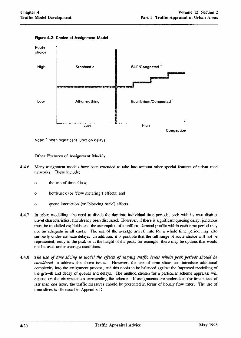
Chapter 4 Traffic Model Development
Volume 12 Section 2 Part 1 Traffk Appraisal in Urban Areas
Figure 4.2: Choice of Assignment Model
Route * choice
High
Low
Stochastic
All-or-nothing
Low
Note: * With significant junction delays.
Other Features of Assignment Models
SUE/Congested *
Equilibrium/Congested *
HIM >
Congestion
4.4.6 Many assignment models have been extended to take into account other special features of urban road networks, These include:
0 the use of time slices;
0 bottleneck (or ‘flow metering’) effects; and
0 queue interaction (or ‘blocking-back’) effects.
4.4.7 In urban modelling, the need to divide the day into individual time periods, each with its own distinct travel characteristics, has already been discussed. However, if there is significant queuing delay, junctions must be modelled explicitly and the assumption of a uniform demand profile within each time period may not be adequate in all cases. The use of the average arrival rate for a whole time period may also seriously under-estimate delays. In addition, it is possible that the full range of route choice will not be represented; early in the peak or at the height of the peak, for example, there may be options that would not be used under average conditions.
4.4.8 The use of time slicing to model the eflects of vaving tr@c levels within peak periods should be considered to address the above issues. However, the use of time slices can introduce additional complexity into the assignment process, and this needs to be balanced against the improved modelling of the growth and decay of queues and delays. The method chosen for a particular scheme appraisal will depend on the circumstances surrounding the scheme. If assignments are undertaken for time-slices of less than one hour, the traffic measures should be presented in terms of hourly flow rates. The use of time slices is discussed in Appendix D.
4120 Traffic Appraisal Advice May 1996
Volume 12 !Section 2 Part 1 Traffic Appraisal in Urban Areas
Chapter 4 Traffic Model Development
Flow Metering and Blocking Back
4.4.9 Most congested assignment models also incorporate procedures for estimating the effects of capacity restrictions on downstream traffic flows (sometimes referred to as ‘flow metering’). This is an important feature of many congested road networks, and failure to take it into account can lead to serious overestimation of queues and delays at downstream junctions and poor estimation of overall network delays. It also leads to the distinction between ‘demand’ flow (i.e. the flow that would exist if there was no upstream capacity restriction) and ‘actual’ flow (after taking such restrictions into account). If this modelling feature is in operation, care must be taken to use the correct flow definition in the subsequent traffic, environmental and economic appraisal calculations (including the validation of traffic flows). Where aggregate flows over a complete model time period (or series of time periods) are being used, the difference will usually be negligible, but if flows for shorter periods are being considered, as for example in certain of the environmental and design calculations, it is the ‘actual’ flow values that are most appropriate (see paragraph 6.2.18 re economic appraisal requirements).
4.4.10 The operation of junctions in urban areas is sometimes influenced by queues blockinn back from an adjacent junction. Most modelling packages have procedures for dealing with this situation, although the success of these varies. The use of ‘blocking buck’ procedures should be considered only where they can be justified in terms of an improved assignment model (in the base year or in a future year). Practical difficulties may arise using blocking back mechanisms at High Speed Merges and the recommended procedure there is described in Appendix E sub-section E6. Elsewhere difficulties sometimes arise when traffic flow estimates produced in the first few assignment model iterations result in an unrealistic application of the ‘blocking back’ procedures. This causes instability in subsequent iterations, and sometimes prevents proper model convergence. One solution that has been found to be effective is to inhibit the ‘blocking back’ effect in earlier model iterations, and to reintroduce it once flows have begun to stabilise.
Route Choice Generalised Cost Coefficients
4.4.11 The travel ‘costs’ referred to in the above paragraphs represent a combination of factors that drivers take into account when choosing routes. Studies have shown that the most important of these factors are time and distance. Where tolls are charged for the use of specific sections of road, these out-of-pocket costs should also be included, preferably allowing for different drivers willingness to pay tolls. This may require separate assignments for each category of driver. Current practice is to calibrate the distance to time weighting to obtain the best assignment (see TAM Sub-Section 9.6). This can be time-consuming.
The recommended procedure is to base the route choice coefficients on HEN2 perceived values, as a starting point, and to carry out a number of sensitivity tests to demonstrate the robustness of the resulting assignment model (including that small changes in Generalised Cost parameters do not lead to large changes in forecast flows).
4.4.12 Since HEN2 provides separate time and vehicle operating cost values for ‘working’ and ‘non-working’ trip purposes, and for different vehicle types, there is a case for treating these separately in the assignment procedures. When ‘all-or-nothing’ or pure ‘stochastic’ assignment techniques are being used this is a simple matter, but for ‘equilibrium’ assignment it is currently only possible with the few software packages that support ‘multiple user class’ assignment methods (see also Paragraph 4.4.25) _ Where assignment of combined purpose matrices is undertaken, weighted average route choice coefficients, using the local purpose mix, should be used, possibly with separate values being specified for each modelled time period, to reflect the different mix of trip purposes.
May 1996 Traftic Appraisal Advice 4121
Chapter 4 Traffic Model Development
Volume 12 Section 2 Part 1 Traffic Appraisal in Urban Areas
4.4.13 Different route choice coefficients can also be used when assigning heavy vehicles. If the assignment model software allows different coefficients to be specified for each road type, these can be used to reflect the fact that most drivers tend to keep to main roads wherever possible, even if there is a modest time/cost penalty in so doing. In the absence of differential coefficients, turn penalties for & movements joining key main routes may need to be considered, while recognising the general advice, that models should be kept as simple as possible, consistent with producing robust results.
Speed-flow Relationships
4.4.14 Speed-flow relationships are widely used in inter-urban trunk road scheme appraisal to model the effects of congestion on travel times and costs. In the core of a congested urban network, all significant junctions will be modelled in detail (simulated) and link-based speed-flow relationships will not necessarily be required for assignment purposes within this core. They are likely to be required for modelling journey times on J& links outside the detailed modelled (simulated) area. Speed Jlow relationships will also be required within the detailed modelled area, for those links where modelledjunctions are not the rn.aill determinant of journey times.
4.4.15 Speed-flow relationships are also used in the economic appraisal of the improvement (for example in COBA - whose relationships based on the latest research are described in Appendix E). The basic principles involved in the use of speed-flow relationships are simple; they represent how link travel costs increase with increasing link flow. The COBA approach is to set a lower bound on the link speed, to represent re-routeing and other effects _ However, this form of speed cut-off is not recommended in a traffic model as it is unlikely to give realistic assignments with congested networks.
Local traffic models, should use speed-flow relationships, based on those in COBA taking full account of local link geometry (particularly width, hilliness and bendiness) as well as road type.
This is particularly important for road links on which flows change as a result of the scheme being evaluated. Local parameters should be calculated for individual routes and distinct sections of routes.
Special speed-flow relationships should only be used in exceptional circumstances, and only then if their use is fully justified and their source is well documented.
4.4.16 Within urban areas the element of delay, associated with queuing at junctions at the end of most links, should be modelled explicitly wherever it is likely to be significant - either in the base year or in future years. Since COBA speed-flow relationships for urban road classes already include an allowance for some junction delays, care must be taken not to include these twice (i.e. on links and at junctions).
In examining the realism of any traffic model output, the areas with the lowest Iink speeds should be examined in conjunction with their implied link speed (ie including both link and junction delay). Very low implied speeds must be individually justified, particularly where they are lower than the equivalent speed cut-offs used in COBA.
4122 Traffic Appraisal Advice May 1996
Volume 12 Section 2 Part 1 Traffic Appraisal in Urban Areas
Chapter 4 Traffic Model Development
4.4.17 Many applications of ‘equilibrium’ assignment involve the Frank-Wolfe algorithm, or some equivalent. This uses an optimisation procedure that in most cases requires speed-flow relationships to be converted to a more analytical form. Typically, this is represented as a power curve:
C(Q) = A + B.(QK&)” for Q i Q,
and C(C)) = C(Q) + queuing delay for Q > Q,
where C(Q) is the cost at flow Q;
Q is the capacity flow; and
Parameters A, B and n describe the relationship between link length, free-flow speed and speed at capacity flow and the parameters reduce as the free flow speed increases. Hence the same power curve is unlikely to apply on links with markedly different free flow speeds.
Speed-flow relationships of the type used in COBA cannot be fitted exactly to this form of curve, since they generally consist of a series of straight lines. The recommended approximation involves adjusting the power curve until a best fit is achieved over the whole range of flows. In this case values of ‘n’ higher than 4.0 should not normally be required.
4.4.18 It ti important that the speed-flow relationship allocated to a particular network link should be as compatible as possible with the base year traflc flows and speeds that actuully occur on that link. If this is not the case, the model cannot be regarded as validated. The same speed-flow relationship should be allocated to each network link for all time periods modelled, unless there are reasons why the speed- flow relationship changes (e.g. parking or bus-lanes).
Model Convergence
4.4.19 In general, the iterative methods for reaching equilibrium, referred to above, will not converge absolutely, and user-defined ‘stopping criteria’ are required to describe the point at which satisfactory convergence is considered to have been achieved. The convergence indicators provided by different software packages
0 vary, as does the availability of a facility for the user to control the assignment process to ensure a given level of convergence. Care needs to be exercised to distinguish between convergence and stability. Stability can often be achieved, indeed some methods force it to happen, without there being convergence to a solution.
4.4.20 Most assignment packages that are suitable for the appraisal of urban road schemes provide one or more of the following five convergence indicators:
0 the number of iterations:
0 the percentage of links on which flows change by less than 5% between successive iterations, sometimes known as ‘P’ ;
0 the difference between the costs along the chosen routes and those along the minimum cost routes, summed across the whole network, and expressed as a percentage of the minimum costs, sometimes known as ‘delta’;
May 1996 Traffk Appraisal Advice 4/23
Chapter 4 Traffkc Model Development
Volume 12 !Scction 2 Part 1 Traffic Appraisal in Urban Areas
0 0 the degree to which the area under the speed-flow relationships is minimised, sometimes known
as ‘epsilon’; and
0 the percentage change in total user costs or time spent in the network between successive iterations, sometimes known as ‘V’ .
The first of these is not recommended for general use, since by itself it gives no indication of the extent to which equilibrium has been achieved. The last should not be used as the main indicator, except when other indicators are not available.
4.4.21 The percentage of links with small flow changes gives a pragmatic view of the degree of convergence, although it is really a measure of stability. It is recommended that, in addition to satisfying the true convergence measures described below, assignment model iterations should continue until at least four successive values of ‘P’ in excess of 90% have been obtained. If this cannot be achieved, especially in a future year assignment, this is an indication of instability caused by the level of traffic demand being higher than can be absorbed by the network capacity.
4.4.22 The ‘delta’ and ‘epsilon’ statistics are better measures of convergence, but are not provided by all packages. They both generally decrease towards a minimum value as the number of iterations increases. ‘Delta’ is preferred, since ‘epsilon’ cannot be calculated when more than one user class is being assigned separately. It is recommended that iterations should continue until the value of ‘delta’ is less than I%, or has at least stabilised. In the latter case supporting information on stability including acceptable values when measured against the other criteria should be provided.
4.4.23 It should be noted that ‘stochastic user equilibrium’ (SUE) assignment converges more slowly than Wardrop (user) equilibrium and, in addition, it is more difficult to monitor convergence. As a consequence:
0 a larger number of iterations will generally be required to achieve a satisfactory level of convergence; and
0 the majority of existing applications of SUE do not calculate ‘delta’ or ‘P’, but rely instead on the number of assignment iterations as the iterative stopping criterion.
There is no reason why ‘delta’ and ‘P’ or similar measures cannot be calculated, but if they are not available the percentage change in total user costs between successive iterations (‘V’) should be used to monitor convergence. In this case, iterations should continue until four successive values of ‘V’ less than 1% have been obtained.
4.4.24 The importance of achieving convergence is related to the need to provide stable, consistent and robust model results. When the model outputs are being used to compare the ‘do something’ and ‘do minimum’ situations, and to estimate the economic benefits of a scheme, it is important to be able to distinguish real differences from those associated with different degrees of convergence. Similar considerations apply when the benefits of different schemes are being compared. Model convergence is therefore the key to robust economic appraisal. Table 4.1 summarises the convergence criteria recommended in the preceding paragraphs which are set out in greater detail in Appendix H. Achieving these criteria may require a different number of iterations in ‘do minimum’ and ‘do something’.
4124 Traffk Appraisal Advice May 1996
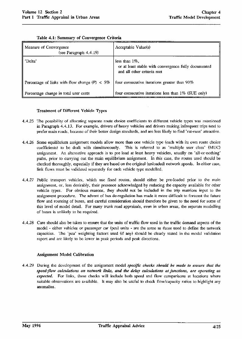
Volume 12 Section 2 Part 1 Traffic Appraisal in Urban Areas
Chapter 4 Traffic Model Development
Table 4.1: Summary of Convergence Criteria
II Measure of Convergence (see Paragraph 4.4.19)
’ Delta’
Percentage of links with flow change (P) < 5%
11 Percentage change in total user costs
Acceptable Value(s)
less than I%, or at least stable with convergence fully documented and all other criteria met
four consecutive iterations greater than 90%
four consecutive iterations less than 1% (SUE only)
TreaIment of Different Vehicle Types
a 4.4.25 The possibility of allocating separate route choice coefficients to different vehicle types was mentioned in Paragraph 4.4.13. For example, drivers of heavy vehicles and drivers making infrequent trips tend to prefer main roads, because of their better design standards, and are less likely to find ‘rat-runs’ attractive.
4.4.26 Some equilibrium assignment models allow more than one vehicle type (each with its own route choice coefficients) to be dealt with simultaneously. This is referred to as ‘multiple user class’ (MUC) assignment. An alternative approach is to pre-load at least heavy vehicles, usually on ‘all-or-nothing’ paths, prior to carrying out the main equilibrium assignment. In this case, the routes used should be checked thoroughly, especially if they are based on the original (unloaded) network speeds. In either case, link flows must be validated separately for each vehicle type modehed.
4.4.27 Public transport vehicles, which use fixed routes, should either be pre-loaded prior to the main assignment, or, less desirably, their presence acknowledged by reducing the capacity available for other vehicle types. For obvious reasons, they should not be included in the trip matrices input to the assignment procedure. The advent of bus de-regulation has made it more difficult to forecast the future flow and routeing of buses, and careful consideration should therefore be given to the need for some of this level of model detail. For many trunk road appraisals, even in urban areas, the separate modelling of buses is unlikely to be required.
4.4.28 Care should also be taken to ensure that the units of traffic flow used in the traffic demand aspects of the model - either vehicles or passenger car (pcu) units - are the same as those used to define the network capacities. The ‘pcu’ weighting factors used (if any) should be clearly stated in the model validation report and are likely to be lower in peak periods and peak directions.
Assignment Model Calibration
4.4.29 During the development of the assignment model specific checks should be made to ensure that the speed-flow culculatiom on network links, and the delay calculations at ~*urtctions, ure operuting us expected. For links, these checks will include both speed and flow comparisons at locations where suitable observations are available. It may also be useful to check flow/capacity ratios to highlight any anomalies.
May 1996 Traffic Appraisal Advice 4125

Chapter 4 Traffic Model Development
Volume 12 Section 2 Part 1 Traffic Appraisal in Urban Areas
4.4.30 At junctions, remedial action should be considered for any turning movement where:
0 the capacity calculated by the model is less than the observed count; or
0 the calculated delays (or queue lengths) are significantly greater than observed delays (or queue lengths).
This will usually involve reviewing the parameters which control the capacity of the movements affected, or possibly reviewing the position of nearby centroid connectors. In some cases the calculation of capacity relates to a group of turning movements, for example where several movements share the same traffic lane(s). For these it is also sensible to make comparisons at the group as well as tbe individual turning movement level.
4.4.3 1 When queue lengths are being compared, careful interpretation is needed of the queue length information output by the model (e.g. how cyclical queues at traffic signals are reported). Comparisons with observed data need to be made on the same basis as those reported by tbe model. Precise validation of queue lengths can be difficult because of the volatility of the observed data.
4.4.32 Once the amendments described in Paragraph 4.4.30 have been made, a second series of adjustments should be considered where:
0 modelled flows are significantly below observed flows for a particular turning movement; or
0 modelled delays (or queue lengths) are unacceptably lower than observed delays (or queue lengths).
The types of adjustment required will be similar to those described above, but in the opposite direction.
Adjustments should only be made to network descriptions if they can be justified and thcsc should be recorded in technical notes.
Arbitrary adjustments to measurable quantities (e.g. link length or junction geometry) should not be made.
Artificial adjustment of link speeds, or link or junction capacities to give a closer frt to observed conditions is not recommended.
Any adjustments made to the base year network during the calibration stage must be checked for ‘logic’ and to determine whether they would apply equally to the future year networks. Particular care should be taken if it is considered that the adjustments may affect the outputs to be used for economic appraisal.
4.4.33 Further checks on the assignment model should be car&d out by inspecting the routes through the network taken by selected traflc movementi. This is complicated by the fact that the capacity restrained assignment procedures used in urban models calculate several sets of routes. The initial set of routes excludes the effects of junction delays, and the paths calculated in subsequent iterations are not representative of the whole assignment. Ideally, a selection of calculated zone to zone routes should be checked for each assignment iteration, particularly if the software package being used can display routes graphically on a VDU screen. Since observations of routes taken are not usually available, tbese checks must be based on local knowledge and the judgement of the modeller, and cannot be regarded as a true validation. Account may need to be taken of the use of ‘signposted’ routes by drivers with limited local knowledge, Remediul action should be taken where unrealistic routes are detected. l
4126 Traffic Appraisal Advice May 1996
Volume 12 Section 2 Part 1 Traffic Appraisal in Urban Areas
Chapter 4 Traffk Model Development
0
4.4.34
4.4.35
4.4.36
4.4.37
a 4.4.38
4.4.39
4.4.40
May 1996 Traffic Appraisal Advice 4127
Assignment Model Validation
It is not possible to validate the assignment model in isolation, since the output traffic flows and travel times will reflect not only the errors in the assignment model, but also those inherited from the input trip matrix and the road network description. This is a particularly important consideration in congested urban areas, where relatively small discrepancies in a trip matrix can have a disproportionate impact on junction delays, and hence on the routes taken by vehicles through the network. On the other hand, since the assignment model is the last part of the modelling process, its output can be used to judge the performance of the model as a whole.
Guidance on the procedures to be used when validating link flows is given in Sub-Section 11.4 of TAM. The choice of links to be validated IIS particularly important, and these should include a reasonable selection of links that carry tra#ic movements critical to the scheme appra&al. Aggregating these links into screenlines provides a powerful demonstration of the overall performance of the model, but in urban areas it is also important to cheek that the model can adequately reproduce observed flows on different types of link during the different model periods (e.g. on ‘rat-runs’ in the peak and inter-peak periods as well as main road links). As indicated in Paragraph 4.4.9, ‘actual’ traffic flows should be used in these comparisons when the assignment model incorporates ‘flow metering’ procedures. The need to use independent count data, from different sites to those used to collect calibration data, is again emphasised. Counts with 95% Confidence Intervals wider than ~15% after conversion to the model base should be separately identified and not normally be used for validation.
In urban areas the performance of the model in reproducing the operating characteristics of road iunctions is also very important, since a high proportion of journey costs (and therefore scheme benefits) is often related to this part of the road network. The choice of junctions to be validated is therefore just as important as the choice of links. Comparisons should be made between modelled turning flows and observed turning counts at key junctions in the study area, including the junctions controlling the most important ‘rat-runs’ and any that are expected to be relieved by the proposed scheme(s) _
The validation of individual turning movements involves a large number of comparisons. This should be presented in order of importance, both geographically and numerically, since the magnitude of turning movements at junctions (and therefore the weight that should be given to individual comparisons), can vary widely. It should also be recognised that the accuracy of the modelled turning flows, in percentage terms, will generally be much less than that of the modelled link flows. In this case, a lesser degree of apparent agreement between modelled and observed flows does not necessarily imply a poorer model fit.
Finally, jorlrnev times should be validated by comparing the observed times to traverse the journey time survey routes with those calculated by the model. This is similar to the network validation check referred to in Paragraph 4.2.9, except that delays at explicitly modelled junctions will have been calculated by this stage.
All of the above validation cotnparisons should be carried out separately for each time period being modelled and specicrl consideration given to compations which vary consistently between periods, and with link flow comparisons being made for each vehicle type included in the model. It is not acceptable to aggregate modelled flows over a 12- or 16-hour period and to present only the validation at that level.
If sub-periods have been defined within peak periods, the comparisons should be considered and presented for the sub-periods and the time period as a whole. If time slices have been defined within peak periods, the comparisons should be presented for the time period as a whole (although the results for individual time slices can often assist in rectifying or explaining any anomalies that occur). Link and turning flows can be aggregated directly, but journey times should either be quoted as a range of values, or as a mean
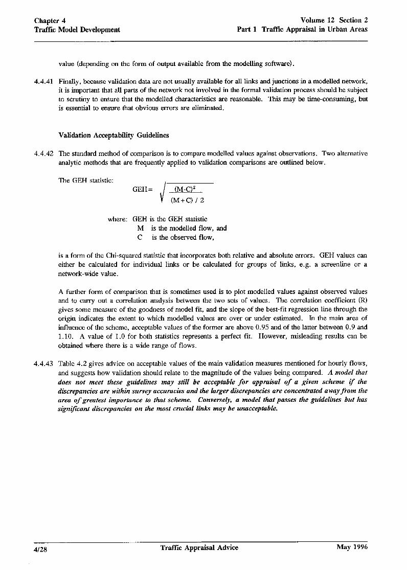
Chapter 4 Traffic Model Development
Volume 12 Section 2 Part 1 Traffic Appraisal in Urban Areas
value (depending on the form of output available from the modelling software) _
4.4.41 Finally, because validation data are not usually available for all links and junctions in a modelled network, it is important that all parts of the network not involved in the formal validation process should be subject to scrutiny to ensure that the modelled characteristics are reasonable. This may be time-consuming, but is essential to ensure that obvious errors are eliminated.
Validation Acceptability Guidelines
4.4.42 The standard method of comparison is to compare modelled values against observations. Two alternative analytic methods that are frequently applied to validation comparisons are outlined below.
The GEH statistic: GEH = (M-C)2
(M+C) / 2
a where: GEH is the GEH statistic
M is the modelled flow, and C is the observed flow,
is a form of the Chi-squared statistic that incorporates both relative and absolute errors. GEH values can either be calculated for individual links or be calculated for groups of links, e.g. a screenline or a network-wide value.
A further form of comparison that is sometimes used is to plot modelled values against observed values and to carry out a correlation analysis between the two sets of values. The correlation coefficient (R) gives some measure of the goodness of model fit, and the slope of the best-fit regression line through the origin indicates the extent to which modelled values are over or under estimated. In the main area of influence of the scheme, acceptable values of the former are above 0.95 and of tbe latter between 0.9 and 1.10. A value of 1.0 for both statistics represents a perfect fit. However, misleading results can be obtained where there is a wide range of flows.
4.4.43 Table 4.2 gives advice on acceptable values of the main validation measures mentioned for hourly flows, and suggests how validation should relate to the magnitude of the values being compared. A mode2 that l does not meet these guidelines may still be acceptible for apprakal of a given scheme 17 the dkcrepancies are within survey accuracies and the larger dkcrepancies are concentrated away from the area of greatest impotfance to that scheme. Conversely, a model that passes the guitlelines but has significant discrepancies on the most crucial links may be unacceptable.
4128 Traffic Appraisal Advice May 1996
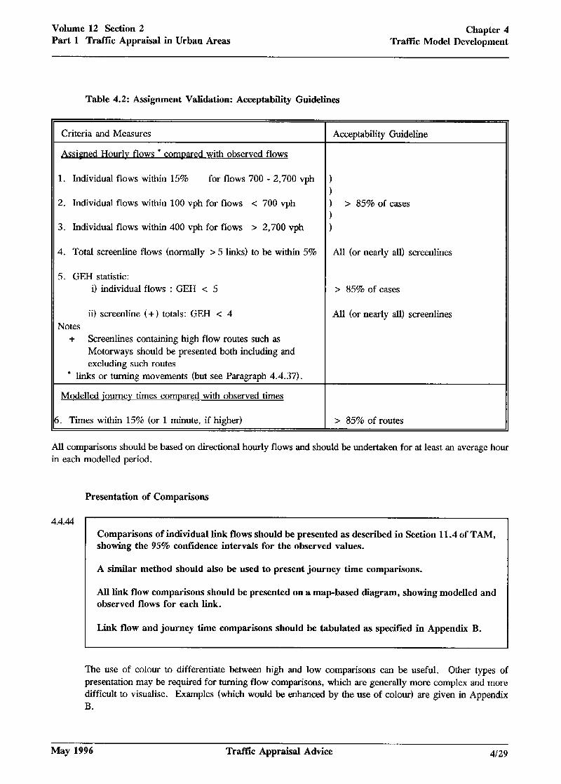
Volume 12 Section 2 Part 1 Traffic Appraisal in Urban Areas
Chapter 4 Traffic Model Development
Table 4.2: Assignment Validation: Acceptability Guidelines
Criteria and Measures
Assigned Hourlv flows * comuared with observed flows
Acceptability Guideline
1. Individual flows within 15% for flows 700 - 2,700 vph ) )
2. Individual flows within 100 vph for flows c 700 vph
3. Individual flows within 400 vph for flows > 2,700 vph
) > 85% of cases
4. Total screenline flows (normally > 5 links) to be within 5% All (or nearly all) screenlines
5. GEH statistic: i) individual flows : GEH < 5 z 85% of cases
ii) screenline (+) totals: GEH < 4 All (or nearly all) screenlines Notes
+ Screenlines containing high flow routes such as Motorways should be presented both including and excluding such routes
* links or turning movements (but see Paragraph 4.4.37).
Modelled iournev times compared with observed times
_ Times within 15% (or 1 minute, if higher) > 85% of routes
All comparisons should be based on directional hourly flows and should be undertaken for at least an average hour in each modelled period.
Presentation of Comparisons
4.4.44 - Comparisons of individual link flows should be presented as described in Section 11.4 of TAM, showing the 95% confidence intervals for the observed values.
A similar method should also be used to present journey time comparisons.
All link flow comparisons should be presented on a map-based diagram, showing modelled and observed flows for each link.
Link flow and journey time comparisons should be tabulated as specified in Appendix B.
The use of colour to differentiate between high and low comparisons can be useful, Other types of presentation may be required for turning flow comparisons, which are generally more complex and more difficult to visualise. Examples (which would be enhanced by the use of colour) are given in Appendix
a B.
May 1996 Traffic Appraisal Advice 4129
--
Chapter 4 Traffic Model Development
Volume 12 Sectioll 2 Part 1 Traffk Appraisal in Urban Areas
4.4.45
4.4.46
4.5
4.5.1
4.5.2
Modelled and observed journey times (along journey time survey routes) can also be compared by plotting cumulative time-distance graphs as shown in Figure B2. This can help in model calibration as it provides a convenient way of identifying the location of any anomalies in the calculation of link or junction delays.
The above techniques, and any others that are considered appropriate, may be used to support validation comparisons. However, they should be used to complement rather than replace the Overseeing Department’s preferred presentation method.
REPORTING REQUIREMENTS
The production of a Local Model Validation Report is a mandatory requirement for trunk road appraisals. Details of the content and format of this report are given in Appendix B. Its purpose is to:
0 demonstrate that the model accurately reproduces an existing, independently observed, situation; and
0 summarise the accuracy of the base from which the forecasts are to be prepared.
In addition to summarising the data used in model development, the LMVR should present details of the network validation, trip matrix validation and assignment validation, in the manner described earlier in this chapter. Technical Notes may be required to provide details of adjustments made in calibrating the model _
4130 Traffic Appraisal Advice May 1996
Volume 12 !3ection 2 Part 1 Traffic Appraisal in Urban Areas
Chapter 5 Traffic Forecasting
a 5 Traffic Forecasting
5.1 ELEMENTS OF FORECASTING
5.1.1 Previous chapters have recommended procedures for developing a base year traffic model for an urban area, and have given details of the types of data that will be required. This chapter describes how the base year model can be developed to produce traffic forecasts for various future situations. The local forecasting procedures recommended by the Department of Transport are outlined in Sub-Section 12.3 of TAM. These are mandatory for trunk road schemes, and their application to urban or peri-urban areas is reviewed in this chapter.
5.1.2 Three basic elements will be involved in all but the most simple traffic forecast. These are:
0 development of future year network descriptions;
0 forecasts of future traffic demand; and
0 assignment. .
Each of these elements is discussed in more detail in the following sub-sections.
5.1.3 In urban areas, special consideration must he given to those parts of the study area where the forecast levels of future traffic demand cannot be accommodated by the proposed future road network. The treatment of such cases is discussed in Sub-Section 5.7.
5.2 FORECAST YEARS
5.2.1 As explained in Sub-Section 2.8, traffic forecasts are required to provide inputs to the economic, operational and environmental appraisals, and these dictate the years for which forecasts should be made. The definition of forecast years will also depend to some extent on the forecasting and appraisal methods used, and the context of the scheme being appraised.
As an absolute minimum, forecasts should be prepared for at least two years, and these should be within one or two years of the anticipated opening and of the 15th year.
5.2.2 Additional forecust yeurs ojlen need to be included to take account o$
0 the inaccuracies introduced into the economic appratial calcuhxtions by interpohting und extrapolating results over more than 10 years within the 30-year evaluhbn period, especially when procedures other than COBA are being used (see also Sub-Section 6.2 of this note) ;
0 yean’ in which any network-based constraints to growth are expected to occur;
0 years in which significant changes are expected to the road network in the model urea (as a result of phased introduction of the scheme, or implementation of other related road schemes) ;
and 0 yeurs in which signtjicunt changes to traJff?c demund in the scheme areu (e.g. new
developments) are expected to occur.
5.2.3 Further discussion of the factors affecting the choice of forecast years can be found in Sub-Section 12.3 of TAM.
May 1996 Traffic Appraisal Advice 5/l
Chapter 5 Volume 12 Section 2 Traffic Forecasting Part 1 Traffic Appraisal in Urban Areas
5.3 FUTURE YEAR NETWORKS
5.3.1 In both the economic and environmental appraisal of road schemes, comparisons are made between the traffic situation (traffic flows, speeds, travel costs, etc.) with and without the scheme, and thi,s requires ‘do minimum’ and ‘do something’ network descriptions. These must be prepared for every year for which a traffic forecast is required.
5.3.2 Special care is required when specz;fying junetin h~yout!s and signal times in both the ‘do minimum’ and ‘do something’ cases, since these are likely to have a significant effect on the performance of future road networks. As with base year networks, it is goodpractice to& as many traflc si@zal times as possible, at least initially, with existing signals retaining the same time as in the base year network description. Reasonable optimisation of signal timings in the ‘do-minimum case is acceptable, to reflect adjustments that would be made to enable the network to cope with the increased traffic flows. These ‘do minimum’ timings should be used as the starting point for optimising the ‘do something’ signal timings. Again, reasonable optimisation in the immediate neighbourhood of the scheme is acceptable, but a different degree of optimisation should be avoided to prevent biassing of the economic evaluation results. For new signal installations, timings may either be fixed at estimated settings or be calculated by the assignment model software, where this facility exists. Further discussion of this aspect of traffic forecasting is included in Sub-Section 5.5, below.
‘Do Minimum’ Networks
5.3.3
5.3.4
5.3.5
‘Do minimum’ networks for each forecast year must be based on the base year network descriptions, and should include all schemes (other than the scheme being appraised) that could reasonably be expected to be in place by that forecast year.
In general, any road scheme in the study area that is included in the trunk road programme, or in local authority transport plans, should be included in the ‘do minimum’ network. However, it will often be desirable to cany out sensitivity tests, excluding those schemes that are subject to zmcertain& Further sensitivity tests may be reqzzired to assess the implications of local transpott policies (e.g. public transporf improvemen& parking policies, traflc calming etc.)
It is also important that minor improvemenfs lo the existing network (e.g. traflc management measures) should be conszilered. The full extent of the improvements required may need to be identified following provisional forecast year assignments that use the ‘do minimum’ network descriptions. In addition, it may be necessary to make assumptions about the geometric and operational characteristics (road widths, junction layouts, signal timings, etc.) of any improvement schemes that are included, especially where they are not defined to the level of detail required by an urban traffic model. In any case, ‘do minimum’ networks must be compatible between forecast years, with the descriptions for succeeding years being based on those for previous years.
Further guidance on the definition of ‘do minimum’ networks is given in Sub-Section 1.2 of the COBA manual, and the treatment of competing and complementary schemes is dealt with in Sub-Section 3.4 of the same document.
512 Traffjc Appraisal Advice May 1996
Volume 12 Section 2 Part 1 Traffw Appraisal in Urban Areas
Chapter 5 Traffic Forecasting
5.3.6
5.3.7
5.4
a 5.4.1
5.4.2
5.4.3
‘Do Something’ Networks
‘Do something’ networks should normally be based on the equivalent ‘do minimum’ network, so that the only difference between the two is the road scheme being appraised. However, where improvements have been included in the ‘do minimum’ network that are intended as an alternative to the scheme being appraised, these must be removed before it is used as the basis for the ‘do something’ network description. Again, a full description of the ‘do something’ network (including geometric and operating characteristics) will be required.
If the introduction of a new scheme is likely to be accompanied by traffic calming at a significant scale, it may be appropriate to test the effects of the scheme both with and without the traffic calming included in the network.
TRAFFIC DEMAND FORECASTS
Forecasts of traffic demand should be based on the validated trip matrices developed for the base year, with separate forecasts being made for each model time period.
The initial estimates of demand may need to be modified to take account of network capacity constraints (see Figure 5.1). Th e application of constraints to growth is discussed in Sub-Sections 5.6 and 5.7.
The methods used to produce traffic forecasts are all based on the application of growth factors, and the following options are generally available:
0 trip end growth factors, preferably by trip purpose, based on the National Trip End Model (NTEM) - or, in some instances, a local trip end model - and applied using a Furness procedure;
0 growth factors derived from a higher tier model; and
0 as a last resort, simple average growth factors based on the National Road Traffic Forecasts (NRTF) .
As indicated below, different methods are appropriate for different circumstances. However, the method adopted should be the simplest that k capable ofproducing a sound forecast. In some cases, different approaches may be followed for different elements of the trip matrix.
National Trip End Model
The National Trip End Model provides trip end and growth estimates (for various car trip purposes) at the local authority District level, up to 2025. In urban areas, traffic growth in peak periods is often different to that in inter-peak periods, partly as a result of a different mix of trip purposes in each time period. The different growth rates for each trip purpose will normally lead to different growth rates for the different time periods.
May 1996 Traffic Appraisal Advice 513
Chapter 5 Traffic Forecasting
Volume 12 Section 2 Part 1 Traffk Appraisal in Urban Areas
Growth Factors
F- Initial Assignments
I I Minor Coding Changes to ---
Relieve Overloaded Junctions ;;z t$.y&s, ;>,: jz
Modify Initial Growth Estimates (where appropriate)
(Peak Spreading etc.)
Intermediate Assignments
Apply Constraints to Traffic Growth :::::: :::::: (cut-offs, matrix capping, elasticity etc.)
Final Estimates of Traffic Demand “g~:~ j :::::: *> i. :“” ,I//,:/ ,,iTjir:,,,:,,:ii,,:,::::i:::: .,,,,,,, ::.:.:~E::::::::::::rr:r.: /,,,,,,,,,,,,,,,,,,,,,,
514 Traffic Appraisal Advice May 1996
Volume 12 Section 2 Part 1 Traffic Appraisal in Urban Areas
Chapter 5 Traffic Forecasting
5.4.4 Where it is necessary to distinguish smaller areas (individual zones or groups of zones) in the analysis, National Trip End Model estimates may be disaggregated. A simple method is to disaggregate according to the proportion of the District’s households (and/or employment places) in each zone, although more refined methods based on local trip end models may sometimes be available.
5.4.5 This approach is especially relevant where differential growth is expected to occur across the model area because of differential land use development. The local planning authority must be consulted to obtain the latest position regarding expected land use changes in the area. However, it is important that the planning data (and other assumptions) used are consistent with those used to produce the National Trip End forecasts. In particular, where the impacts of spe@ic developments are included in the calculations, these shouhi be accommodated within the Dk.trkt totals.
When aggregated to District level, the resultant trip end growth must match that derived from the National Trip End Model (NTEM) estimates. I 1 a
In exceptional cases, where the introduction of a large development is expected to influence the distribution of population and/or employment over a wide area, and the development was not included when the land use data were incorporated in the latest revision to the NTEM, control totals may be derived by aggregating the National Trip End Model estimates over more than one District.
In addition, for trips to or from zones away from the area of immediate interest, it is permissible to use aggregations of district level data (e.g. at County level) to derive the growth rates.
5.4.6 To maintain compatibility with NRTF forecasts, all growth factors must be based on (or constrained to) estimates from the National Trip End Model. The latest values should be used and they must be adjusted by applying the appropriate National Forecast Adjustment Factor (NFAF).
5.4.7 Further details of NRTF, the National Trip End Model and NFAF are given in Chapters 7 and 12 of TAM1. It should be noted that the overseeing Departments have adopted these forecasts to ensure that a common set of assumptions is used in the appraisal of trunk road schemes, and occasionally rebate them to take account of more recent actual traffic growth. The most recent rebasing including revised NFAFs is incorporated in the computer program TEMPRO which was issued for England and Wales with HETA Guidance Note l/94 entitled “National Trip End Model - May 1994 Projections”. Future rebased forecasts are expected to be issued as a Part of DMRB Volume 12. To reflect the uncertainties involved in traffic forecasts, two sets of assumptions are normally used, one reflecting ‘high’ growth and the other reflecting ‘low’ growth.
Both ‘high’ and ‘low’ growth assumptions must be applied for each forecast year, when using any of the traffic forecasting methods outlined in tbis section.
0 ' These refer to the latest National Road Traffic Forecasts (Great Britain) 1989, published in 1989 by HMSO.
May 1996 Traffic Appraisal Advice 5/s
Chapter 5 Traffuz Forecasting
Volume 12 Section 2 Part 1 Traffic Appraisal in Urban Areas
Growth Factors from Higher Tier Models
5.4.8 While the use of local or national trip end models takes some account of the re-distribution effects resulting from differential land use changes, neither method deals with the full range of re-distribution and modal shift effects that can sometimes accompany the introduction of a new road scheme, major public transport schemes or changes in transport policies. If any of these effects is thought to be significant, growth factors derived from a higher tier model which reflecti these factors may be applied to provide forecast& from the base year matrices. These factors may also provide initial estimates of network-wide capacity constraint effects. They must be applied separately to each set of time period (and. if appropriate, trip purpose) matrices.
If this approach is adopted, the higher tier model must have been thoroughly validated.
This validation must confirm that the input assumptions (e.g. land use, economic growth and car ownership) to its forecasts are consistent with those in the National Trip End Model (with NFAF)/NRTF.
5.4.9 In practice, the derivation and application of suitable growth factors from a higher tier model may not be straightforward. Various approaches involving different degrees of sophistication are possible. It is normally necessary to check that the growth factors derived do not contain any anomalies. Some adjustment of extreme values may be required.
NRTF Growth Factors
5.4.10 The growth estimated by the NRTF is a national average level of growth. Furthermore, in urban areas, traffic growth in peak periods is often different from that in inter-peak periods. This is partly the result of a different mix of trip purposes, and the fact that growth rates derived from trip ends tend to be different for each purpose type.
For these reasons, the use of simple NRTF forecasts is not applicable for ear trips in urban areas.
Unless a suitable local trip end model exists, however, it is the only method that can be applied to goods vehicles, since these are not covered by the National Trip End Model.
516 Traffk Appraisal Advice May 1996
Volume 12 Section 2 Part 1 Traffic Appraisal in Urban Areas
Chapter 5 Traffic Forecasting
l 5.5 ASSIGNMENT
5.5.1 Separate runs of the assignment model are required for each combination of forecast year, network (‘do minimum’ or ‘do something’), model time period and growth level (‘high’ or ‘low’).
In general, the assignment procedures used for forecasting must be the same as those used in the validated base year model. However, a number of external assumptions and factors need to be reviewed. These include:
0 the criteria used by drivers when choosing routes;
0 assignment model convergence requirements; and
0 the proportions used to distribute the total number of trips in each peak period between time slices (where applicable) _
Route Choice Criteria
5.5.2 As indicated in Sub-Section 4.4 of this note, the route choice criteria used in the base year model should be based on a combination of time and distance costs, derived initially from values contained in Highways Economics Note 2 (HEN2). The advice given in Sub-Sections 12.3 and 12.5 of TAM is that these route choice parameters should be retained for all future years. However, since values of time and fuel costs are predicted to increase at different rates in future, and this will tend to change the way drivers balance time and distance savings, TAM recommends that sensitivity tests should be carried out to investigate the implications of this course of action.
Convergence Requirements
5.5.3 For forecast years, the convergence requirements of congested assignment models are similar to those for the base year, and similar values should be achieved wherever possible. The requirements are set out in Appendix H. It is particularly important that the levels of convergence achieved in the ‘do minimum’ and ‘do something’ assignmenfs are similar, and that they are su$iciently stringent to ensure that differences in the resulfs are not confused with oscillation effecti within the model. Adopting the criteria set for the base year model will generally be sufficient to ensure that this is the case, although this may require more iterations for the do minimum than for the do something. Where difficulties are experienced in achieving adequate levels of convergence, this is usually an indication that the network is overloaded and the remedial action outlined in Sub-Section 5.7 will be required.
May 1996 Traffic Appraisal Advice 517
Chapter 5 Traffic Forecasting
Volume 12 Section 2 Part 1 Traffic Appraisal in Urban Areas
Assignment Model Checks
5.5.4 TJie assignment model output for each forecast year must be inspected careficl~ to ensure that the resulti are realistic. Any problems with the ‘do minimum’ situation should normally be dealt with before assignments are carried out for the ‘do something’ cases. Turning flows, overall link transit times, flow changes on fixed-speed links and the flows predicted on new network links should all be checked. It is also important that &l modelled junctions are carefully checked, especially where the economic appraisal will depend on journey times and delays taken from the traffic model. Examples of the problems that might arise at this stage include:
0 unreasonable delays at individual junctions on the existing road network, or on new road schemes introduced into the ‘do minimum’ or ‘do something’ networks, even after ‘peak spreading’ has been taken into account;
0 junctions at which the traffic demand for any turning movement (or group of turning movements) exceeds the available capacity over the model period taken as a whole;
0 traffic queues increasing through a model period, resulting in excessive residual queues at the end a
of the time period; or
0 zones for which the number of arriving and departing trips exceeds the estimated parking capacity (usually in town centres and other urban activity areas).
The actions that should be taken in each case are discussed below.
Overloaded Junctions
5.5.5 The capacity of individual overloaded junctions should be reviewed to ensure that the network codi,ng is reasonable. Where minor (traffic management) changes to existing junction geometry would reduce overall queues and delays (and these are not incompatible with wider considerations e.g. safety, amenity and local authority policies), these should be implemented in the network descriptions, and reported in an appendix to the Forecasting Report. The proposed designs for new road schemes (and sometimes their wider implications in terms of increased traffic demand elsewhere in the study area) also need to be reviewed in the light of the assignment results. Finally, if unrealistic (and incorrect) coding of the base year network is revealed by any of the forecast year traffic assignments, this must be corrected, and its impact on model validation investigated and reported.
Traffic Appraisal Advice May 1996
Volume 12 Section 2 Part 1 Traffic Appraisal in Urban Arcas
Chapter 5 Traffic Forecasting
l 5.6 INITIAL ADJUSTMENTS TO DEMAND
Parking Demand
5.6.1
5.6.2
5.6.3
Controlling parking demand to the estimated number of available parking spaces involves comparing the forecasts of vehicle trip ends in areas such as town centres with the most likely future supply of spaces. The likely turnover in parking spaces for the period being modelled must enter into the calculations, and this will be different for long-stay, short-stay and private parking spaces. These techniques are particularly important in urban areas where local authority policy is to limit traffic demand by the management of parking spaces. Where future parking capacity is uncertain, sensitivity tests should be carried out.
In areas where parking demand exceeds the estimated supply of spaces, consideration should be given to reallocating a proportion of trips to different zones in or around the town centre (to represent drivers having to walk further), or possibly to out-of-town zones containing park-and-ride car parks. This reallocation can be weighted to reflect the use of appropriate alternative parking facilities on the approaches to town centres, and can sometimes be automated by modelling walk or park-and-ride links. Care should be taken, however, to monitor the way such links are used within the assignment model.
Peak Spreading
As congestion increases in urban road networks, there is a tendency for the distribution of traffic during peak periods to become more uniform, as journeys are delayed or deliberately re-timed to avoid the worst parts of the peak periods. This phenomenon is sometimes referred to as ‘peak spreading’ _ Conversely, when a new road scheme introduces additional capacity to a road network, the effect can be temporarily reversed (‘peak contraction’). These effects can be reflected in the traffic model by adjusting the proportions used to allocate peak period trips to time slices. The calculations involved are often based on subjective judgement, but more objective methods, based on empirical data, have recently been developed. Further details of these are given in Appendix F.
It is important that these initial adjustments to demand are made, and that steps are taken to adjust the capacity of the road system to realistic levels (see paragraph 5.5.5) before more comprehensive constraints are considered to reduce traffic demand levels within the model.
5.6.4 Where any of the problems outlined in Paragraph 5.5.4 still persist, however, the application of growth constraint methods may be unavoidable. In some cases initial growth estimates from a higher tier model, which may already contain some constraint, may need to be capped further. Possible techniques for achieving this are described below.
May 1996 Traffic Appraisal Advice 519
Chapter 5 Traffic Forecasting
Volume 12 Section 2 Part 1 Traffk Appraisal in Urban Areas
5.7 CONSTRAINTS TO GROWTH
5.7.1 For scheme appraisal, the traffic flows output by the assignment model must be as realistic as possible, and must reflect the extent to which the capacities of both the ‘do minimum’ and ‘do something’ networks constrain traffic growth. A constrained forecast may still be the most likely outcome, despite the additional capacity provided by the scheme, and if so it would be the most relevant for design and environmental appraisal purposes.
5.7.2 ‘Variable trip matrix’ economic appraisal methods (see Sub-Section 6.2) increase the requirement For the traffic flows output by the assignment model to be as realistic as possible. They too must reflect the extent to which network capacities constrain traffic growth. Finally ‘fixed trip matrix’ economic appraisal, which requires the use of the same matrix for the ‘do minimum’ and ‘do something’ situations, usually need to be constrained to the level of growth that can be accommodated by the ‘do minimum’ network.
5.7.3 The above considerations are especially important in large urban areas, where it is not always possible to accommodate fully the forecast levels of unconstrained traffic demand. Several practical methods have been developed to apply the necessary constraints. These include:
0 user-determined factors and cut-offs;
0 matrix capping techniques;
0 elasticity techniques;
0 incremental loading techniques; and
0 shadow network techniques.
The term ‘growth constraint methods’ is used here to refer to the techniques as a whole; the term ‘matrix capping’ is only used in the context of those methods to which it strictly applies.
5.7.4 Further details of the methods involved, including a comparison of their advantages and disadvantages, are given in Appendix G following recent research into appropriate methodologies.
The realism of any growth constraint techniques used must be demonstrated and their USC justified. The simplest method should be chosen to suit the needs of the current scheme appraisal.
5.7.5 The application of such techniques may be regarded as a proxy for more complex influences on future travel patterns (re-distribution, modal shift, trip suppression, etc.), and may not be justified (or required at all) if growth factors have been derived from a higher tier model that already takes such effects into account. Whatever techniques are used, the degree of constraint that is appropriate will require the exercise of considerable judgement.
5/10 Traffic Appraisal Advice May 1996

Volume 12 Section 2 Part 1 Traffic Appraisal in Urban Areas
Chapter 5 Traffic Forwasting
a 5.7.6 Whichever method is adopted, the following principles must be adhered to:
0
0
0
a
0
0
the method must be applied con.Gtently to ‘do minimum’ and ‘do something’ networks;
constraints shot&l ensure that as far as possible appropkte traflc queue, speed and dehy criteria are met. Appropriate criteria should have regard to:
i) ii) iii)
present day values, whether extreme values are confined to a few locations or are widespread, guidance in Sub-Section 6.4 of the COBA Manual where the average delay per vehicle for any turning movement at a junction is limited to 5 minutes in peak periods and 3 minutes in inter-peak periods;
the constrained demand in each modelled time pen’od should be compatible with the capacity of the network being considered; residual queues at the end of each time period should be within reasonable limits and spill-over effects to adjacent time periods should not be permitted (This reinforces the need for time slicing (see Appendix D) within an appropriate choice of peak periods) ;
separate consideration must be given to each time period, since the impact of limited capacity on traffic growth will be greater in peak periods than in inter-peak periods; the methods used must be able to assess the situation over each complete model period, even when separate assignments are being carried out for a number of time slices within the period;
separate consideration should also be given to the different vehicle types represented in the model, if this is considered appropriate;
forecast years should be constilered in chronological order, since constraints to growth will be incremental over time; (in this context, high and low growth assumptions still apply; the constraint criteria are the same for both growth scenarios, which may lead in extreme cases to a common ultimate peak period matrix - the difference being the year in which the constraint criteria are realised;
no ortgin to destination movement should exhibit negative growth (i.e. be less than its base year value), or growth sign@cantly in excess of the unconstrained growth level being considered - ‘high’ or’ low’ - unless these can be justified in terms of land use, re-distribution, modal shift changes, or policy considerations;
the rest& must reflect reasonable expectations of behaviour in the light of thepredicted pattern of congestion;
the methods used must enable checks (and intervention) to be carried out at each stage; and
checks should be made to ensure that the relative levels ofpeak and inter-peak traflcpredicted by these methods are sensible.
May 1996 Traffic Appraisal Advice Wll
Chapter 5 Traffic Forecasting
Volume 12 Section 2 Part 1 Traffic Appraisal in Urban Areas
5.8 REPORTING REQUIREMENTS
5.8.1 It is essential that the methods used to forecast future tmflc levels, and the assumptions made, are$@ documented in a Forecasting RepoH. In particular, specific reference must be made to:
0 the changes made to the base year network description to produce the ‘do minimum’ networks (including a schedule of assumed minor traffic management changes, and the effect on validation of any corrections to the coding of the base. year network);
0 the changes made to the ‘do minimum’ networks when constructing the ‘do something’ networks;
0 the methods and assumptions used to forecast traffic demand for future years (including the steps taken to ensure compatibility with national forecasts);
0 justification and description of any procedures used to restrain traffic growth to realistic levels within the model;
0 the degree of convergence achieved in the various forecast year assignments; and
0 a full account of all checks carried out on the assignment results (including link transit times and junction delays, where relevant), together with details of the results throughout the network.
5.8.2 Further guidance on the contents and format of the Forecasting Report are given in Appendix C.
5/12 Traffic Appraisal Advice May 1996

Volume 12 Section 2 Part 1 Traffic Appraisal in Urban Areas
Chapter 6 Use of Traffic Model Outputs in Scheme Appraisal
a 6 Use of Traffic Model Outputs in Scheme Appraisal
6.1
6.1.1
GENERAL
Traffic appraisal is not an end in itself, but provides important inputs to other aspects of the appraisal of a road scheme. The purpose of this chapter is to review the various forms of appraisal involved and, in particular, to highlight any issues relating to the use of traffic model outputs in those appraisals.
6.1.2
61.3
6.2
6.2.1
6.2.2
6.2.3
Three principal types of appraisal are required for a trunk road scheme, namely: economic appraisal, environmental impact assessment and operational appraisal. In addition, the traffic model will be expected to provide information for use in the design of the road and its associated junctions. Each of these aspects of appraisal is addressed below.
Urban traffic models that take account of ‘flow metering’ (that is the effect of bottlenecks on traffic flow profiles downstream of the bottleneck) sometimes make a distinction between ‘demand’ flows and ‘actual’ flows. In most of the aspects of appraisal covered by this chapter it is the ‘actual’ flow outputs that should be used, (but to ensure that all the traffic is accounted for see Paragraph 6.2.18), If the guidance given in Sub-Section 5.7 has been followed, the ‘demand’ and ‘actual’ flows accumulated over each model time period as a whole, should be very similar.
ECONOMIC APPRAISAL
The Department of Transport maintains and releases three standard computer programs for economic appraisal (COBA, URECA and QUADRO) _ The Scottish Office maintains and releases its own economic appraisal program (NESA) . Although these use common economic assumptions to calculate the benefits associated with a particular road improvement, they are intended for use in different circumstances. Full details of the principles and operation of the programs (summarised below) are given in their respective user manuals, which are ultimately to be issued as Volumes 13, 13A, 13B & 14 of the Design Manual for Roads and Bridges (DMRB). Since NESA is broadly equivalent to COBA, no separate description is given here. Further details of NESA can be found in Volume 13A of DMRB.
Fixed and Variable Matrix Methods
A fundamental assumption made when using fixed matrix based COBA, NESA and URECA is that the economic appraisal should be undertaken on the basis that the origin to destination trip matrix will be unchanged as a result of the scheme - the so-called ‘fixed trip matrix’ approach. This simplifying assumption is conservative in many situations, but may oversimplify the situation for larger schemes that have a more extensive impact on travel patterns (or schemes that are elements of wider strategies) _ Details of where the assumption is inappropriate are set out in the Guidance on Induced traffic (DMRB ~12.2).
The ‘fixed matrix’ approach implies that any constraint to traffic growth imposed by the capacity of the ‘do minimum’ network within the 30-year economic appraisal period, must be treated as a fixed constraint for the economic appraisal of the ‘do something’ case. This may not be appropriate in urban areas, if the additional capacity provided by the scheme allows significant additional growth to occur beyond the ‘do minimum’ constraint.
May 1996 Traffic Appraisal Advice 6/l

Chapter 6 Use of Traffic Model Outputs in Scheme Appraisal
Volume 12 Section 1 Part 1 Traffic Appraisal in Urban Arcas
6.2.4 Where appropriate, the alternative ‘variable matrix’ approach, in which different ‘do minimum’ and ‘do something’ trip matrices are used, should be adopted. This is discussed in Sub-Section 1.7 of the COBA manual. Although it has not yet been fully implemented in standard COBA or URECA programs, the Department has issued guidance on ways of using current programs and test versions to undertake variable matrix economic appraisals, Zf ‘variable matrix’ methods are considered appropriate for the economic appratial of a trunk road scheme, this must be d&used at an early stuge with the overseeing organkation’s Project Manager and the advice provided in the Guidance on Induced traflc (DMRB 1712.2) should be followed.
6.2.5 Whichever approach is considered appropriate, in urban areas a choice has to be made between:
0 using the default COBA calculations, and accepting the simplifications involved;
0 using COBA more flexibly, and providing the necessary justifications for local inputs; or
0 inputting the results of traffic assignments directly into URECA, supported by more extensive justification and checking of input data.
The following paragraphs discuss each of these options in more detail
COBA
6.2.6 COBA has been used for many years to provide a standardised economic appraisal of road schemes in different parts of the country. It is principally concerned with calculating:
0 travel time costs;
0 vehicle operating costs; and
0 accidents costs.
These costs are accumulated over all network links and are calculated for both ‘do minimum’ and ‘do something’ networks, the difference representing the net benefit to road users arising from the scheme. This requires the definition of ‘do minimum’ and ‘do something’ networks, as described in Sub-Section 5.3.
6.2.7 The main traffic inputs required by COBA are:
0 the traffic flow on each network link;
0 vehicle type data; and
0 traffic growth, by vehicle type.
Complementary information on link characteristics are also input, covering road width, hilliness, bendiness, road type etc and this allows traffic speeds to be calculated from standard speed-flow relationships. Junction delays for key junctions are calculated from layout data which also needs to be specified. If vehicles speeds fall below a specified level, or junction delays exceed a specified maximum a cut-off on these values is introduced by COBA.
612 Traffic Appraisal Advice May 1996
Volume 12 Section 2 Part 1 Traffic Appraisal in Urban Areas
Chapter 6 Use of Traffic Model Outputs in Scheme Appraisal
l 6.28 In a standard run of COBA, traffic flows may be input in any one of the following ways:
0 annual average hourly traffic (AAHT);
0 the average 16-hour weekday traffic flow (0600 to 2200) in a neutral month; or
0 the average lZ-hour weekday traffic flow (0700 to 1900), again in a neutral month.
Hence, the traffic flows from the main traffic model need to be aggregated to give the chosen basis for input to a standard COBA. User-defined or average factors are then used to convert these to AAHT.
6.2.9 To take account of variations in the level of traffic flow, the 8,760 hours of the year are divided into different groups, referred to as ‘flow groups’, each representing a specific level of flow over a given number of hours. In the standard (or default) specification of COBA, the number of hours represented by each flow group is fixed, and the relative flow levels and vehicle mixes associated with each group are determined by a network-wide classification which takes into account national data and the local ratio of
0 average August to neutral month flows - known as the ‘seasonality index’. COBA then synthesises the flow for each network link and junction, by flow group, using the input flows referred to above.
6.2.10 In cases where traffic characteristics in the scheme area (flow variation, vehicle type and journey purpose mix, vehicle occupancy, etc.) are significantly different from the average default values, COBA allows a more flexible approach to the specification of traffic flow inputs. This facility could be used more widely in urban areas in recognition that the input data provided to a standard COBA run, and its default assumptions may be an over-simplification for many urban road networks, as the factors affecting variations in link flow and traffic composition are generally more complex than the national default values.
6.2.11 By inputting parameters for the AM peak, PM peak and inter-peak periods COBA runs can be carried out separately for these periods (and their associated shoulder periods) directly from the traffic model. In such cases, the number of hours in the year to be represented by each modelled time period should be determined by reference to the results of a year’s continuous ATC monitoring on key routes in the scheme corridor. Average traffic flows for the remaining (night-time and quiet weekend) hours should be derived using local flow group factors applied to all day or preferably the inter-peak modelled flows, using information obtained from the ATC data specified above, or less satisfactorily default flow group factors from COBA.
6.2.12 The approach in the previous paragraph allows more account to be taken of any differential growth that may occur in future years (between inter-peak and peak periods, for example), and for the impact of any differential growth cut-offs that may apply. A complementary, but already more common feature is the use of user-supplied values for the mix of vehicle types (cars, LGV, OGVl, OGV2 and PSVs) and the proportion of car trips in work time specified by input parameters which override the default values used by the program.
6.2.13 Within COBA, traffic flow figures for each year in the 30-year appraisal period can be derived from base year values, using national or user-specified local growth profiles (by vehicle type) relating to ‘high’ and ‘low’ growth assumptions. The arguments put forward in Chapters 4 and 5 suggest that neither of these standard approaches may be realistic in urban networks, because:
0 the capacity limitations of urban road networks will tend to limit traffic growth before the end of the 30-year period;
0 traffic patterns may change in future, and the use of ‘rat runs’ will tend to increase, as congestion increases: and
May 1996 Traffk Appraisal Advice 613
Chapter 6 Use of Traffic Model Outputs in Scheme Appraisal
Volume 12 Section 1 Part 1 Traffic Appraisal in Urban Areas
0 traffic growth will differ by journey purpose, and will therefore vary by time of day
To overcome some of these deficiencies, COBA permits and the overseeing Departments encourage the approach set out in paragraph 6.2.11 and the input of revised traffic flows at intermediate years in the 30- year appraisal period. These may require additional forecast year model runs, as discussed in Sub-Section 5.2.
62.14 Although the above refinements overcome many of the criticisms of the standard COBA approach, they do not allow full use of all the information available from the traffic model.
URBCA
6.2.15 In 1986 SACTRA, in its report ‘Urban Road Appraisal’, identified the need to make direct use of the traffic flows and journey times produced by the traffic appraisal in the calculation of economic benefits. The main reason given was that COBA makes its own estimates of journey times and delays, without reference to those output from the detailed traffic appraisal. The result was seen as an unnecessary inconsistency between the information provided by the traffic model and that used in the economic appraisal.
6.2.16 The Government’s response accepted this recommendation in the case of urban traffic models that use congested assignment techniques, and that model different traffic conditions and different times of day separately. The URECA program was subsequently issued to allow these principles to be put into effect.
URECA is usually considered to be more appropriate where, at any time during at least the first 20 of the standard 30-year economic appraisal period:
0 there is likely to be interaction between junctions, for example with the degree of congestion at one affecting the degree at another;
0 a significant proportion of network links will be operating at or above the congested end of their speed-flow relationship, and the cut-offs implied by the COBA speed-flow relationship would dominate the calculation of benefits; and/or
0 ignoring ‘flow metering’ effects would have a significant impact on the calculation of delays, and would distort the assessment of scheme benefits.
Choosing to use UBECA should not be seen as an ‘easy option’. Extensive justification of the inputs is necessary, andaestimatcd journey times and junction delays require careful checking to ensure that the times and delays input to UBECA are sensible. This external checking is necessary because UBECA makes none of the checks used by COBA and places no restrictions on its inputs.
6.2.17 URECA uses the same basic economic assumptions as COBA and is intended to be as compatible as possible with COBA. Traffic flows, speeds and delays are taken directly from the traffic model (via a suitable interface program). This information must be input for each forecast year, model time period and vehicle type, and the number of hours for which each data set contributes to the total annual situation must be specified. Interface programs which facilitate this process are the responsibility of the owners of the congested assignment packages and may eventually facilitate easier checking of URECA input data, by identifying outliers and presenting data required for the checks.
614 Traffic Appraisal Advice May 1996
Volume 12 Section 2 Part 1 Traffic Appraisal in Urban Areas
Chapter 6 Use of Traffic Model Outputs in Scheme Appraisal
6.2.18 Where time slices (or sub periods) are defined within a peak period, there is a facility to use the separate traffic model outputs for each time slice. To ensure that all queuing traffic is properly accounted for, the ‘actual’ flows should be used for the earlier time-slices and the ‘demand’ flows for the final time-slice (less any endemic queues input as a pre-load to the first time-slice) _
6.2.19 URECA calculates costs and benefits for the years for which traffic data are provided, and derives values for intervening years by interpolation. Traffic levels are extrapolated as necessary to a full 30 years assuming they remain constant for years following the last year for which data are provided (although the values of the economic parameters continue to grow). Hence, the recommendations for choosing forecast years are generally the same as for COBA, but a sufficient number of intermediate forecast years must be included in the appraisal for the interpolation to be realistic. As congestion delays vary non-linearly over time, and interpolation and extrapolation over long periods can give biased results, neither interpolation nor extrapolation should cover periods greater than about 10 years.
6.2.20 The URECA method of calculating scheme benefits, can only be justified in preference to COBA. if its traffic model output is used without modification and is demonstrably reliable. If interface programs introduce any inconsistency between the traffic and economic models (such as a delay cut-off in one and not in the other) the methodology fails to meet the fundamental concerns expressed by SACTRA, and reported in paragraph 6.2.15, making COBA preferable because of its greater consistency between schemes.
6.2.21 The reliability of any traffic model used in conjunction with URECA must be checked thoroughly prior to use. It is important that interface programs or manual checks on traffic model outputs are used at an early stage to highlight any extreme values so that the assignment model can be refined as necessary to eliminate any need for delay cut-offs. Since URECA places no restrictions on its input values this must be a separate activity and a more extensive checking procedure than for a model used in conjunction with COBA. The speed-flow reIatiomh@ andjunction dehzy relationsh@s used in the trafic model, are ubo effectively user-deflned, and also should be fitillly justfied.
The URECA method depends on the reliability of traffic model output. Hence,
0 these outputs must be checked thoroughly prior to use, particularly to ensure that model speeds and calculated junction delays are within realistic limits.
0 Interface programs must not impose delay cut offs.
6.2.22 All 8,760 hours of the year must be represented in the URJXA model. This wiIl require several modelled time periods. The number of hours in the year represented by each modelled time period should be determined by reference to the results of a year’s continuous ATC monitoring on key routes in the scheme corridor. Assumptions may be used at early stages of scheme development, provided that by Order Publication stage and subsequently, local ATC data is used and all 8,760 hours are represented.
May 1996 Traffic Appraisal Advice 615
Chapter 6 Use of Traffic Model Outputs in Scheme Appraisal
Volume 12 Section 1 Part 1 Traffic Appraisal in Urban Areas
The benefits associated with some of the quiet time periods and at weekends can be significant and ignoring them can seriously underestimate the overall economic benefit of the scheme. Nationally on built-up roads 20% of annual traffic travels in the busiest 24 hours of the weekend, 62% during the busiest 60 weekday hours and typically 18% of annual traffic travels during the 84 quietest hours of each week.
6.2.23 The analyst must consider the local importance of weekend traffic. In most cases weekend daytime traffic levels will be lower than during the week, travel patterns will usually be different and traffic congestion more localised. Analysts should consider the suitability of the weekday inter-peak model for weekend daytime traffic (with or without scaling the inter-peak trip matrices). In other cases separate weekend modelling is likely to be needed.
6.2.24 For night-time traffic at weekends and on weekdays it will usually be adequate to scale down the inter- peak trip matrices and assign the mean hourly flow.
6.2.25 When scaling matrices to represent weekends and other periods care must be taken to ensure that the scaling is appropriate to all areas in which significant benefits arise and that any differential growth, or growth cut-offs, are not carried forward to the off-peak/weekend period, unless this can he justified. Local scaling factors obtained from ATC data shou1.d always be used when available and presented as shown in Figure Dl.
6.2.26 In the early stages of scheme appraisal, the following assumptions (similar to COBA default values) may be a good starting point, pending the availability of better information:
0 peak period flows may be assumed to occur on 250 days per year, for P hours modelled per day;
0 inter-peak flows may be assumed to cover (4,380 - 25OP) hours per year: and
0 overnight and other low flow periods may he assumed to cover 4,380 hours per year.
6.3
6.3.1
6.3.2
DELAYS AT ROADWORKS
QUADRO and alternatives
The QUADRA program is specifically intended for use in the economic assessment of traffic delays during scheme construction and also maintenance operations during the life of the scheme. However, experience has shown that QUADRO is not appropriate for assessing delays caused by roadworks or construction works in urban or peri-urban areas, because it is not able to model. junctions and it is not always possible to represent complex diversions using the single diversion route method employed in QUADRO.
Construction and maintenance activities in urban areas are likely to have a significant effect on traffic behaviour over a wide area. Carriageway width restrictions, voluntary and compulsory diversions and changes to junction layouts/operation) are all likely. These types of traffic management can be modelled best using the same congested assignment package as used to predict the other traffic effects of a scheme. Several network descriptions may be required to describe the road layouts and conditions in operation for different stages of construction _
616 Traffic Appraisal Advice May 1996
Volume 12 Sxtion 2 Part 1 Traffic Appraisal in Urban Areas
Chapter 6 Use of Traffic Model Outputs in Scheme Appraisal
6.3.3 The economic assessment of traffic delays during scheme construction, and both ‘do minimum’ and ‘do something’ maintenance operations during the life of the scheme, should then be carried out using the same appraisal package used to assess the other economic effects of the scheme (usually URECA), taking into account the length of time for which each road layout is likely to be in place,
6.3.4 Drivers’ responses to modified road conditions are usually determined by the duration and scale of the disruption caused by the roadworks. They are likely to range:-
from a) drivers continuing to travel the same route as in the base case regardless of any delay caused by the roadworks. This ‘No Re-Routeing’ behaviour is likely to be the most significant behaviour for one or two days after the roadworks have been introduced and the converse effect is likely to be the most significant behaviour after long term major roadworks finish, that is traffic patterns take several days to return to a more normal situation;
to b) drivers re-routeing throughout the whole network, where individuals attempt to minimise their journey time. This response occurs when roadworks have been in place for some time. Modelling this behaviour assumes implicitly that enough drivers who are adversely affected by roadworks are aware of alternative routes, and of the alternative conditions on those routes;
and c) drivers retiming the start of their journey, changing their destination or mode, not making the trip (trip suppression) etc.
6.3.5 The combination of drivers responses make the prediction of traffic delays difficult especially for the first few days of the works. Hence for the long duration construction operations and major maintenance works (for example resurfacing and reconstruction) it is considered reasonable to model responses b) and c) and ignore a) when running the traffic model.
6.3.6 Congested assignment traffic models are typically run for 3 hour periods and the results growthed up to represent a full day/week/year using expansion factors based on an appreciation of the hourly traffic patterns over the network being modelled. To reflect response c), alternative expansion factors would need to be calculated to represent expected conditions during the duration of the roadworks and any seasonal optimisation in the planned programming of the roadworks. The principles set out in paragraphs 6.2.21 to 6.2.25 should be adopted to ensure that the full duration of the roadworks is modelled.
6.3.7 Roadworks in urban areas are increasingly being carried out during inter-peak periods and (if environmentally acceptable) during the night. If the analyst is aware of the exact periods when the works are to take place, then the traffic model should be run just for these periods. If works are restricted wholly to night-time and the road capacity available to traffic is always greater than the demand, then it may be reasonable to assume zero roadworks delay costs.
May 1996 Traffic Appraisal Advice 617
Chapter 6 Use of Traffic Model Outputs in Scheme Appraisal
Volume 12 !?+ection 1 Part 1 Traffic Appraisal in Urban Areas
6.4 ENVIRONMENTAL IMPACT ASSESSMENT
6.4.1 Guidance on the appraisal of environmental impacts of trunk road proposals is contained in Volume 11 of the Design Manual for Roads and Bridges (DMRB) . The main aspects of the environmental assessment that are related to traffic flow include:
0 traffic noise:
0 air quality;
0 impact on vehicle travellers; and
0 pedestrians, cyclists, equestrians and community effects.
6.4.2 The main traffic data requirements cover flow, composition and speed. These are discussed below, with particular reference to the contribution made by traffic model outputs, As with the economic assessment, the environmental assessments often involve comparisons between the ‘do minimum’ and ‘do something’ situations _
a
The traffic information required for the main environmental assessments should be based on, or assessed from, trafic model outputs, wherever possible. In general, ‘high’ traffic growth forecasts should be used for these calculations, taking into account any growth constraints associated with the n&work being considered, where appropriate.
Alternative calculations based on ‘low’ traffic growth may also be made as a sensitivity test, if required.
Traffic Flow
6.4.3 For the assessment of the environmental impacts, 18-hour (06.00 to 24.00) AAWT and AADT flows are normally required, together with annual average peak hour flows. These traffic flows will need to be built up from individual model time period data for the appropriate forecast years, with flows for parts of the day that have not been modelled specifically being infilled by factoring. Further factoring will be required to convert the seasonal base used for the traffic model to annual average conditions.
a 6.4.4 Current flows are required, together with forecast values for the year of opening and the 15th year.
Occasionally, forecasts for an intermediate year may also be required.
Traffic Composition
6.4.5 The basic requirement is the proportion of goods vehicles (COBA classifications OGVl and OGV2) on each network link and in each of the traffic flow periods outlined above. For modelled time periods this can be estimated from model outputs, with average values for longer periods being estimated from several model outputs. Additional information will be required to estimate values for any periods not included in the traffic model.
6.4.6 Other characteristics of the vehicle fleet may also be relevant (e.g. the percentage of diesel cars), but national data for these can usually be applied.
618 Traffic Appraisal Advice May 1996

Volume 12 Section 2 Part 1 Traffic Appraisal in Urban Areas
Chapter 6 Use of Traffic Model Outputs in Schcmc Appraisal
6.4.7
6.5
l 6.5.1
6.5.2
6.5.3
Traffic Speed
Average traffic speeds are required for each link in the ‘do minimum’ and ‘do something’ networks, for each forecast year being considered. Where the period to which the average speed relates needs to cover more than one model time period, the average speed should be calculated from a weighted average, obtained from several model outputs. The influence of junction queues and delays on overall link speeds will also have to be considered in congested urban areas.
OPERATIONAL APPRAISAL AND SCHEME DESIGN
Operational Assessment
In urban areas, the characteristics of a road scheme which need to be assessed will include the width of carriageway to be provided between junctions, and the type and size of the junctions themselves. Several model runs with different scheme designs and junction types (roundabouts, traffic signals, at-grade, grade- separated) will be required at appropriate forecast years, to determine the most effective combination of features. Consideration should also be given to the impact on the surrounding road network, including possible locations where additional improvement measures might be required to facilitate effective operation of the scheme itself.
When carrying out this operational assessment, the following measures of effectiveness should be considered:
0 average traffic speeds (by direction at a link level and also at a network total level);
0 the location and extent of queues and delays (at junctions, and other bottlenecks) ;
0 volume to capacity ratios (on links);
0 ‘stress’ points (or areas); and
0 any implications for accessibility to or from particular locations (e.g. shops, hospitals etc.).
The traffic model should be able to produce all the outputs necessary for this assessment. Further details of the requirements, and appropriate presentational techniques, are discussed in Chapter 13 of TAM.
Geometric Design
Standards for both road and junction designs in urban areas are expressed in terms of peak hour flows in the fifteenth scheme year. The historic approach was to calculate the 3Oth, 50th and 200th highest hourly flows (in a year) and default tidalities and use these as the basis for design. Congested assignment models are now sufficiently well developed to replace this historic approach, particularly when one of the modelled hours chosen is representative of the 50th highest hourly flows. ‘Ihis can often be achieved by the use of peak hour flows in a neutral month
May 1996 Traffic Appraisal Advice 619

Chapter 6 Use of Traffic Model Outputs in Scheme Appraisal
Volume 12 Section 1 Part 1 Traffic Appraisal in Urban Areas
6.5.4 While the traffic model is a useful tool for assessing the area-wide impacts of a particular scheme (or its individual components), care must be taken to ensure that my detailed model outpu/s used in the design process are senstile. In particular, the limitations of the traffic mtiel must be recognised, and adjustments made where required.
Checks of the final selected design of key links and junctions should be undertaken, using the procedures set out in the relevant design manuals. The ability of the design to handle predicted traffic flows in both peak periods must also be demonstrated.
6.5.5 Any significant layout or operational changes made as a result of these checks should be reflected in the traflc model. Sensitivity tests with both ‘high’ and ‘low’ traffic growth should be carried out to demonstrate the range of operational solutions that might be appropriate.
Pavement Design
6.5.6 The traffic information required for pavement design relates to the cumulative number of million standard axles (msa) that will pass over the pavement during its design life. The flow of commercial vehicles (i.e. OGVl + OGV2 + PSV, as defined in Paragraph 2.7.2) is the most significant factor in these calculations, and this may be estimated from the traffic model outputs, if required. The ‘high’ tra@ic growth forecasts should be used in th& calculation.
References
6.1. Incidents and Recovery Procedures at Major Roadworks. TRL Project Report, unpublished 1993.
6/10 Traffic Appraisal Advice May 1996
Volume 12 Section 2 Chapter 7 Part 1 Traffic Appraisal in Urban Areas Enquiries
0
7. Enquiries
All technical enqumes or comments on the Advice should be sent in writing as appropriate to:
;. Head of Highways Economics and Traffic Appraisal Division (HETA) I, Ix 11 Department of Transport c\ Great Minster House T WORSLEY 76 Marsham Street Head of Highways Economics and London SWlP 4DR Traffic Appraisal Division
I
The Director of Roads The Scottish Office Development Department Victoria Quay Edinburgh EH6 6QQ
J INNES Director of Roads
The Director of Highways Welsh Office Y Swyddfa Gymreig Government Buildings Ty Glas Road Llanishen Cardiff CF4 5PL
K.. J xLm4q
K J THOMAS Director of Highways
Road Service Headquarters Clarence Court lo- 18 Adelaide Street Belfast BT2 SGB
D O’HAGAN Assistant Technical Director
May 1996 Traffic Appraisal Advice 7/l
Assistant Technical Director of Road Services Department of the Environment for Northern Ireland
Volume 12 Section 2 Part 1 Traffic Appraisal in Urban Areas
Appendix A Report of Traffk Survey
a
Al
Al.1
Al.2
a Al.3
A2
A2.1
A2.2
a
Appendix A - Report of Traffic Survey
GENERAL REQUIREMENTS
This appendix outlines what is required in the presentation of the Report of Traffic Surveys (i.e. the traffic data collection work undertaken specifically for the appraisal of the scheme) _ This report should present the data in a factual manner, to inform the reader about what data have been collected, their accuracy, and their relevance to the scheme.
All data should be presented, perhaps in summary form, and should be accompanied by estimates of accuracy (full details of the data should also be available for inspection, where requested). The data presented should be accompanied by a commentary, highlighting features of importance, defects, anomalies, etc.
Details of the source, location (illustrated on a map), method of collection (e.g. roadside interview, automatic count, etc.), date, day of week and duration of collection must be given, together with information on where any fuller data is held.
TRAFFIC FLOW DATA
Flow data (i.e. data collected by automatic traffic counters, manual classified counts, etc.) should, where possible, be presented in the form of histograms or graphs illustrating daily, weekly, seasonal and long term variations, all sub-divided by vehicle type. Figure Dl shows one form of summary presentation. Supporting tabulations should also be provided and, where appropriate, these should distinguish between and compare different times of day (e.g. AM peak, PM peak or inter-peak).
Turning counts at simple junctions should be presented in tabular form, with separate sub-totals of the total flow on each approach arm. Flows should again be classified by vehicle type and time period. Junction locations should be shown on a map and adequate geographical information should be provided to allow junction layouts and individual junction arms to he identified. For complex junctions a diagram is likely to be required. Flows which are significantly different from their opposite movement in their opposite peak period should be highlighted. A complex example is reproduced as Figure Al.
A3 ORIGIN TO DESTINATION DATA
A3.1 Origin to destination data (i.e. data collected on movements between points, by roadside interview or other techniques) should be presented in the form of tabulations and ‘desire line’ diagrams (or other, similar, forms of presentation) illustrating observed movements between sectors. An example is reproduced as Figure A2. These should distinguish between different times of day and, wherever possible, between the main vehicle types and journey purposes represented in the study area. An alternative presentation is shown in Figure Bl. In that case diagrams illustrating the location of sectors must be provided. The graphical presentations should be supported by tabulations indicating the sample size, response rates (in the case of postcard interviews) and sample factors applied at each survey site, by vehicle type and time period. The tabulations should also include measures of the accuracy of the data.
May 1996 Traffic Appraisal Advice All
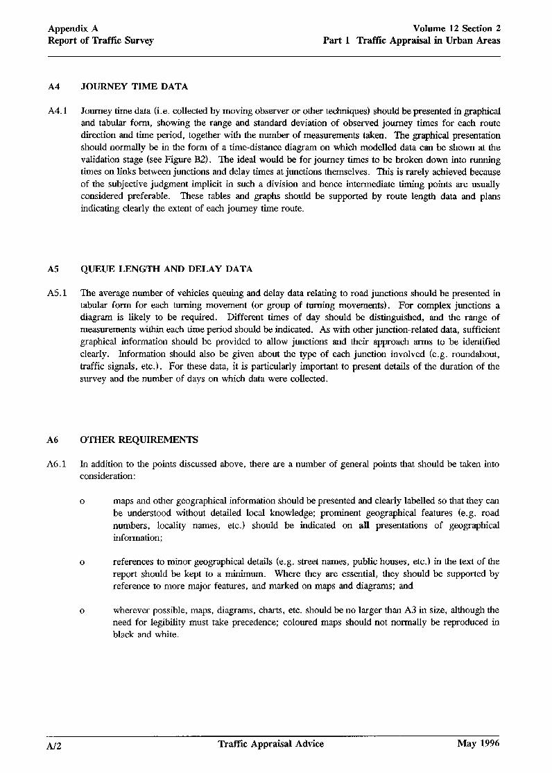
Appendix A Report of Traffic Survey
Volume 12 Section 2 Part 1 Traffk Appraisal in Urban Areas
A4 JOURNEY TIME DATA
A4.1 Journey time data (i.e. collected by moving observer or other techniques) should be presented in graphical and tabular form, showing the range and standard deviation of observed journey times for each route direction and time period, together with the number of measurements taken. The graphical presentation should normally be in the form of a time-distance diagram on which modelled data can be shown at the validation stage (see Figure B2). The ideal would be for journey tunes to be broken down into running times on links between junctions and delay times at junctions themselves. This is rarely achieved because of the subjective judgment implicit in such a division and hence intermediate timing points are usually considered preferable. These tables and graphs should be supported by route length data and plans indicating clearly the extent of each journey time route.
A5 QUEUE LENGTH AND DELAY DATA
A5.1 The average number of vehicles queuing and delay data relating to road junctions should be presented in tabular form for each turning movement (or group of turning movements). For complex junctions a diagram is likely to be required. Different times of day should be distinguished, and the range of measurements within each time period should be indicated. As with other junction-related data, sufficient graphical information should be provided to allow junctions and their approach arms to be identified clearly. Information should also be given about the type of each junction involved (e.g. roundabout, traffic signals, etc.). For these data, it is particularly important to present details of the duration of the survey and the number of days on which data were collected.
A6 OTHER REQUIREMENT3
A6.1 In addition to the points discussed above, there are a number of general points that should be taken into consideration:
0 maps and other geographical information should be presented and clearly labelled so that they can 0 be understood without detailed local knowledge; prominent geographical features (e.g. road numbers, locality names, etc.) should be indicated on all presentations of geographical information;
0 references to minor geographical details (e.g. street names, public houses, etc.) in the text of the report should be kept to a minimum. Where they are essential, they should be supported by reference to more major features, and marked on maps and diagrams; and
0 wherever possible, maps, diagrams, charts, etc. should be no larger than A3 in size, although the need for legibility must take precedence; coloured maps should not normally be reproduced in black and white.
Traffic Appraisal Advice May 1996
West Way
South Street The Crescent
<zF> Node Number
Light vehicles Heavy vehicles
Flows are in vehicles per hour
260 420 25 40
170 165 rt 15 15
Volume 12 Section 2 Appendix A Part 1 Traffic Appraisal in Urban Areas Report of Traffk Survey
West Way
\
<TiG-->
Note: Holloway Street
Light vehicle flows which are more than 20% different from their
opposite movement are shaded.
I Figure Al. Presentation of Turning Flows
May 1996 Traffic Appraisal Advice A/3

Appendix A Report of Traffic Survey
Volume 12 Section 2 Part 1 Traffic Appraisal in Urban Areas
Figure A2. Presentation of Desire Line Data
Observed Major Traffic Movements June 1992
III1 III1
0 500 1000
AM Peak Period 8 - 9 am
IIIIIIIII
0 500 1000
PM Peak Period 5- 6Pm
Traffic Appraisal Advice May 1996
Volume 12 Section 2 Part 1 Traffic Appraisal in Urban Areas
Appendix B Local Model Validation Report
l
Bl
B1.1
B1.2
B2
B2.1
B2.2
l
Appendix B - Local Model Validation Report
GENERAL
The Local Model Validation Report (LMVR) serves two broad purposes. l?irst, it summarises the accuracy of the base from which forecasts are to be prepared. This is required because the accuracy of forecasts is directly related to the accuracy of the base. Second, where modelling methods have been used, the LMVR should demonstrate that the model accurately reproduces an existing, independently observed, situation. This is needed to give confidence in the results produced by the model when used in forecasting mode.
The preparation of a Local Model Validation Report is mandatory for trunk road schemes.
The LMVR provides an invaluable reference document, especially if further model development work is to be carried out at a later date. However, there will usually be a need for additional reference material to provide fuller details of the model development. This should be contained in Technical Notes and other appropriate documentation.
REPORT STRUCTURE
The structure of the LMVR should be as follows:
0 a description of the model used and its development (including evidence of the fit achieved to the calibration data, and a description of any sensitivity tests undertaken, and their results) ;
0 a description of the data used in building and validating the model;
0 evidence of the validity of the network employed;
0 a validation of the trip matrices employed;
0 a validation of the trip assignment;
0 a validation of any other special features (e.g. higher tier model inputs, trip end models, modal choice models, etc.) employed; and
0 a present year validation, if appropriate.
Although this structure, and the weight given to the various elements within it, may be adapted to suit each scheme, no item should be omitted. The following paragraphs outline the material required in each element. Examples of diagrams illustrating ways of depicting the validation comparisons of flows and link transit times are attached to this appendix (see figures Bl to B5) _
May 1996 Traffic Appraisal Advice B/l
Appendix B Local Model Validation Report
Volume 12 Section 2 Part 1 Traffic Appraisal in Urban Areas
B3
B3.1
B4
B4.1
B4.2
El.5
B5.1
B5.2
B5.3
MODEL DESCRIPTION
The description of the model and its development should include the following:
0 the type of model used, together with reasons for selecting that model;
0 the geographical extent of the model area and the region surrounding it, together with information to confirm that it is appropriate for the scheme being considered;
0 the time periods and vehicle types modelled, with appropriate justifications (where time slicing methods are being used, information should also be given about the derivation of the trip matrices applicable to each time slice) ;
0 the methods used to calibrate the model, together with details of the calibration data and a summary of the calibration results; and
0 where applicable, the software package and programs used.
In this context, the term ‘model’ should be taken to cover all manipulations of data.
DESCRIPTION OF DATA
All data used in calibrating and validating the model should be presented in summary form, together with the associated measures of accuracy. Details of the source, location (illustrated on a map), type (e.g. roadside interview, automatic count, etc.) duration, day of week, time of day and date of collection should be presented, making reference to the relevant Report of Traffic Survey. Where data are factored, measures of accuracy should be provided for the factors, and both the original and factored data values should be presented. Calibration data (used in model development) should be presented quite separately from validation data.
Where the same type of data is available from more than one source (whether collected by the same method or a different method), a comparison should be made and the degree of agreement reported.
NETWORK CHECKS
The modelled highway network should be clearly shown on a map base, and the ‘internal’ and ‘external’ model areas should be clearly marked. Where congested assignment models have been used, the locations of junctions where delays have been explicitly modelled should be shown. Network diagrams should also illustrate the location of zone connectors.
The coding of speeds on the network should be reported, indicating whether fixed or flow-related speeds have been used. Where both types have been used, a map illustrating the location of each type should be provided.
The coding of other network characteristics (eg carriageway width) should also be reported.
B/2 Traffic Appraisal Advice May 1996
Volume 12 Section 2 Part 1 Traffic Appraisal in Urban Areas
Appendix B Local Model Validation Report
a B5.4
I36
B6.1
B6.2
a
B6.3
B7
B7.1
B7.2
B7.3
Network checks, involving an examination of an initial set of routes, should be supported by diagrams illustrating the routes chosen, together with any other evidence that they are reasonable. Checks of network speeds and other characteristics should also be presented by making comparisons with observed journey time data. A separate presentation should be made for each time period being modelled.
TRIP MATRIX VALIDATION
Each step in the assembly of base year trip matrices should be reported separately, giving details of the methods used, assumptions made, factors applied and a summary of resulting sector to sector movements. A clear distinction should be made and details drawn to the readers attention between movements based on recent, reliable observations and those infilled synthetically or from other sources.
Matrix validation should be presented at sector to sector level, with additional details for critical zone to zone movements. Comparisons should made for each time period and, where possible, vehicle type. Where independent origin to destination data are not available for validation purposes, comparisons should be based on independent counts at suitable screenlines and cordons.
The sectors used in the above analyses should be illustrated on map-based plans. An example of an overlay version is shown in Figure Bl.
TRIP ASSIGNMENT VALIDATION
The key outputs from the traffic appraisal are the forecast traffic flows and, particularly where economic appraisal methods other than COBA are to be used, the link transit times and junction delays on the network. For this reason, and because it often reflects deficiencies in earlier stages, validation of the assignment is of great importance. The selection of links and junctions for validation should ensure that all important movements are validated. Assignment validation can provide valuable insights into other aspects of the model, such as zoning and networks, and should be designed to do that as far as possible.
Assignment validation results for flows, link transit times and, where appropriate, junction delays, should be presented in three forms:
0 tables, including locations, types of observation, observed values and 95% confidence limits, assigned values and the difference between assigned and observed values as a percentage of the observed;
0 in diagrammatic form, illustrating the relationship between assigned values and the 95% confidence range of the observations (examples are given for journey time comparisons in Figures B2 &. B3) ; and
0 on map-based network diagrams showing assigned and observed values, differences and the 95% confidence range of observations (examples are given for modelled flow comparisons in Figures B4 to B6).
Separate presentations should be prepared for each modelled time period, and evidence should also be presented that the vehicle types distinguished in the model are adequately represented. All such presentations should include sub-totals for cordons and screenlines, and any other appropriate aggregation. The units of traffic flow used must be clearly stated.
May 1996 Traffic Appraisal Advice B/3
Appendix B Local Model Validation Report
Volume 12 Section 2 Part 1 Traffic Appraisal in Urban Areas
e B7.4 Where the assignment represents a time slice within a tune period (e.g. the peak hour within the peak
period), separate presentations should also be prepared for the whole tune period. Flows may be expressed as a total for the period or as an hourly average (the report should clearly state which), and transit times and delays should be weighted averages.
B7.5 Where iterative assignment techniques have been used, the report should give information about the level of convergence achieved - as per Appendix H, and the path towards the final state.
BS VALIDATION OF OTHER FEATURES
B8.1 Where there are other unusual features in the appraisal, these should be described carefully and fully validated. A brief description should be given of any existing models that have been used (e.g. higher tier models), and full documentary evidence included of their local validation, accompanied by adequate references to their data sources and overall validation.
B9 PRESENT YEAR VALIDATION
B9.1 A present year validation should be presented when the model is based on data more than five to six years old, or when there is reason to believe that conditions have changed since the data were collected. The present year validation should demonstrate that the model can accurately reproduce the present year situation, given the changes that have taken place since the data were collected. It should cover the same topics as the base year validation.
BlO OTHER REQUIREMENTS
BlO. 1 In addition to the points discussed above, there are a number of general points, applicable to all elements, that should be taken into consideration:
0 in all elements of the LMVR, attention should be given to the quantification of both the model estimates and their accuracies; wherever possible, statistical measures of accuracy should be presented; a
where estimates with measures of accuracy are to be presented, the presentation should include the estimate itself and its upper and lower 95% confidence limits; the units used should always be stated;
maps, network and zone plans and other geographical information should be presented and clearly labelled so that they can be understood without detailed local knowledge; prominent geographical features (e.g. road numbers, locality names, etc.) should be indicated on all presentations of geographical information;
0 references to minor geographical details (e.g. street names, public houses, etc.) in the text of the report should be kept to a minimum. Where they are essential, they should be supported by reference to more major features, and marked on maps and diagrams; and
0 wherever possible, maps, diagrams, charts, etc. should be no larger than A3 in size, although the need for legibility should take precedence. Coloured maps should not normally be reproduced in black and white. a
B/4 Traffic Appraisal Advice May 1996
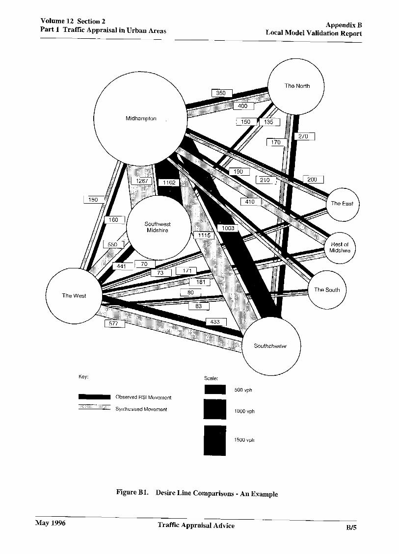
Volume 12 Section 2 Part 1 Traffk Appraisal in Urban Areas
Appendix B Local Model Validation Report
Midhampton
Southchester
Key:
m Observed RSI Movement
Synthesised Movement
Scale:
m 500vph
1000 vph
Figure Bl. Desire Line Comparisons - An Example
May 1996 Traffic Appraisal Advice B/5
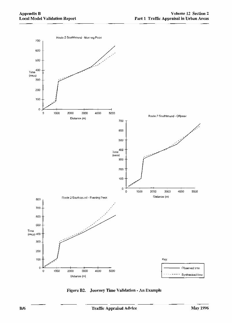
Appendix B Local Model Validation Report
Volume 12 Section 2 Part 1 Traffk Appraisal in Urban Areas
Route 2 Southbound - Morning Peak
T
500
Tirne400 (sets)
2000 3000
Distance (m)
800 -
700 --
600 --
500 --
Time (sec.) 400 --
300 -̂
200 --
100 --
Route 2 Southbound - Evening Peak
600
500
Time400 (sets)
300
200
Key:
I 2000 3000 4000 5000
Distance (m) II
Figure B2. Journey Time Validation - An Example
Route 2 Southbound _ Offpeak
2000 3doo
Distance (m)
Traffic Appraisal Advice May 1996
1600
1400
1200
1000
Time (sets) 800
400
200
b b
b
3
Observed Mean Journey
Time
Synthesised 4 Mean Journey
Time
Length of vertical line represents the 95% confidence limits around the observed mean journey time. Text shows direction of bias outside confidence limits.
I I
Volume 12 Section 2 Appendix B Part 1 Traffic Appraisal in Urban Areas Local Model Validation Report
Low High High Low Low
Route
Figure B3. Journey Time Validation - An Example
May 1996 Traffic Appraisal Advice B/7
Appendix B Local Model Validation Report
Volume 12 Section 2 Part 1 Traffk Appraisal in Urban Areas
Key: 180, -20, -11 .I Observed flow, flow difference, percentage difference
Morning peak hour link flows in 1991
Figure B4. Plot of Flow Differences - An Example
B/S Traffic Appraisal Advice May 1996
Volume 12 Section 2 Part 1 Traffic Appraisal in Urban Areas
Appendix B Local Model Validation Report
New Road\ / \ . . . ..onarl\ 1 860 1 830 1 \
/ pJew I \“--
/
2601 280
250 1 300
Vicarage Road -
780 1 950
\ Eastern Road /
A - Observed Morning Peak Hour (two-way) link flows in October 1991
B -Assigned Morning Peak Hour (two-way) 1991 link flows
C
D 3 Confidence Interval for observed flows
pj&j Flows outside Confidence Interval are shown shaded
Figure B5. Base Year Link Flow Validation - An Example
May 1996 Traffic Appraisal Advice

Appendix B Local Model Validation Report
Volume 12 Section 2 Part 1 Traffic Appraisal in Urban Areas
AM Peak Hour 8 - 9am
PM Peak Hour 5 - 6pm
Key:
1. Flows are in vehicles 2. Flows are for November 1991
except where indicated otherwise
Figure B6. Base Year Link Flow Validation - An Example
B/10 Traffic Appraisal Advice May 1.996
Volume 12 Section 2 Part 1 Traffic Appraisal in Urban Areas
Appendix C Forecasting Report
Appendix C - Forecasting Report
Cl GENERAL REQUIREMENTS
Cl _ 1 The purpose of the Forecasting Report is to document the methods and assumptions used in preparing the traffic forecasts and to present the forecasts themselves. The report should demonstrate that the forecasts are consistent with the Department’s National Road Traffic Forecasts (NRTF). It should also describe the impact of local factors derived from NTEM and NFAF and show how they have been taken into account. The report should present the forecasts that form the basis of the economic, environmental and other appraisals, together with the basis and results of any sensitivity tests that may have been carried out.
Cl .2 The emphasis placed on these reporting requirements will vary, depending on the current stage of scheme
a
assessment. At the early stages (in England - Public Consultation (PC) and Preferred Route (PR)), more than one route alignment and/or scheme layout will usually be considered. At the Order Publication (OPR) stage the forecasts will generally only relate to one route (layout), although the traffic information required will often be more detailed than in previous stages. When the Forecasting Report refers to a stage in which more than one option is being considered, the results of all options, including those that are rejected, should be presented.
c2 STRUCTURE OF REPORT
C2.1 The structure of the report should be as follows:
0 a description of the methods and assumptions used in forecasting future traffic demand;
0 a description of the ‘do minimum’ and ‘do something’ networks examined: and
0 a presentation of the ‘do minimum’ and ‘do something’ traffic forecasts.
C2.2 Although the content of each element within this structure may be adapted to suit each scheme, no item should be omitted. The following paragraphs outline the material required in each element.
C2.3 Because the LMVR and Forecasting Report are complementary, the Forecasting Report should not repeat information given in the LMVR, unless that information is required in the Forecasting Report.
May 1996 Traffic Appraisal Advice C/l
Appendix C Forecasting Report
Volume 12 Section 2 Part 1 Traffic Appraisal in Urban Areas
c3 DESCRIPTION OF METHODS
C3.1 The description of the methods used to forecast traffic demand should include the following:
0 the use made of the Department’s national zonal trip end projections, including details of the level of disaggregation (e.g. District, County or Region); the calculations should be set out in tabular form, providing details for both ‘low’ and ‘high’ growth;
0 where Districts are disaggregated into finer zones, details of the methods used should be given, and a sample calculation included; the description should make clear how the constraint to the District level growth rate is achieved; the source of any additional data used should be given, and the data summarised in the report;
0 the handling of future land use developments should be fully documented in the report, and the way they are accommodated within the District control totals should be demonstrated;
a
0 if growth is limited by network constraints, full details of the timing and degree of constraint should be provided, together with the methods employed and the results obtained; and
0 the overall study area growth rates should be presented in the Forecasting Report, and compared with the NRTF rates; results should be presented for both ‘low’ and ‘high’ growth forecasts.
c4 NETWORK DESCRIPTIONS
C4.1 Changes to the highway network (excluding the scheme itself) should be divided into those that are fully committed and those that are less certain, and the latter examined individually using appropriate sensitivity tests. Descriptions of network changes should be supported by maps illustrating the locations of those changes.
C4.2 The route of the scheme itself, and of any alternatives considered, should be ihustrated on a map. Where the characteristics of junctions affect the forecast traffic patterns, sufficient details should be provided to enable the effects to be understood.
c/2 Traffic Appraisal Advice May 1996

Volume 12 Section 2 Part 1 Traffic Appraisal in Urban Areas
Appendix C Forecasting Report
C5 PRESENTATION OF TRAFFIC FORECASTS
C5.1 The Forecasting Report should include details of traffic forecasts with both the ‘do minimum’ and ‘do something’ networks, for all years for which forecasts are explicitly prepared and for both ‘low’ and ‘high’ growth assumptions. The information that will be used in the economic analysis should be presented first. For COBA, this means the traffic flow on maps covering &l links; & for other procedures, link times (for aJ links) and junction delays (for &l modelled junctions) should also be presented. A second and separate presentation should be made of any forecasts different from that used in the economic appraisal (e.g. where different units or time periods are required, or where ‘fixed matrix’ assignments have been used in the economic appraisal) _ These must provide full details of the traffic flow and speed and delay information that is to be used for environmental assessment and scheme design purposes.
C5.2 In both cases, this information should be presented in the form of maps, supported where necessary by tables. Traffic flow information should be segregated by vehicle type, if appropriate, and the units used should be clearly stated. Separate information should be given for each model time period, and the methods used to factor model outputs to cover other time periods should be clearly indicated. Where several schemes are being compared, the information should be presented in such a way as to facilitate comparison between them.
C5.3 The traffic flow forecasts should be supported by load relief diagrams, indicating the absolute and percentage changes in traffic flow that are expected on completion of the scheme, and selected link analyses, based on the trips using the key link (or links) on the scheme. Again, comparisons between options should be facilitated. An example is shown in Figure Cl. If methods other than COBA are to be used for economic appraisal, changes in link transit times and junction delays should be presented in a similar manner.
C5.4 When iterative assignment methods are used, the level of convergence achieved should be reported and compared with those achieved in the base year assignments.
C6 OTHER REQUIREMENTS
a C6.1 In addition to the points discussed above, there are a number of general points applicable to all elements of the report, that should be taken into consideration:
0 maps, network and zone plans and other geographical information should be presented so that they can be understood without detailed local knowledge; prominent geographical features (e.g. road numbers, locality names, etc.) should be indicated on all presentations of geographical information;
0 references to minor geographical details (e.g. street names, public houses, etc.) in the text of the report should be kept to a minimum. Where they are essential, they should be supported by reference to more major features, and marked on maps and diagrams; and
0 wherever possible, maps, diagrams, charts, etc. should be no larger than A3 in size, although the need for legibility must take precedence. Coloured maps should not be reproduced in black and white.
May 1996 Traffuz Appraisal Advice c/3

Appendix C Forecasting Report
Volume 12 Section 2 Part 1 Traffic Appraisal in Urban Areas
4399
--\
Key: I
Do-minimum Reduction in flow Percentage Reduction
Flows are AADT vehicles
Increase in flow
Figure Cl. Load Relief Diagram - An Example
c/4 Trafk Appraisal Advice May 1996
Volume 12 Section 2 Part 1 Traffic Appraisal in Urban Areas
Appendix D The Use of Sub-periods and Time SIiccs
Dl
D1.l
a D1.2
D1.3
D2
D2.1
a D2.2
D2.3
Appendix D - The Use of Sub-periods and Time Slices
INTRODUCTION
It is easiest, in assignment modelling, to assume ‘steady state’ conditions throughout the modelled period. This basic assumption implies that both the pattern of demand, as represented by the trip matrix, and the level of demand stays constant throughout the period to which the assignment relates. In practice, flow levels are likely to vary within peak periods and in congested areas delays are also likely to vary. Consequently, the assumption of a uniform demand profile within each time period may prove inadequate and the use of the average arrival rate for a whole time period may seriously under-estimate average delays _
Ideally, at the start of the peak period, there should be no significant queues (see Paragraph 2.5.4 in the main report). As demand increases, queues are likely to build up, as a result of limited capacity and, if so, there could be “flow-metering” and/or “blocking back” effects which cause drivers to choose different routes at the “peak of the peak” _ The combination of these effects is likely to result in a range of route choice options some of which would not be used under average conditions.
These effects are likely to be particularly significant in congested urban areas and should be taken into account by means of “time slicing” the peak period.
TRIP MATRICES
Appropriate terminology must be used to explain the extent of non uniformity which is being modelled. To that end, throughout this advice, the distinction has been drawn between time slices (where the O-D pattern remains the same but the traffic volumes differ) and sub-periods (where the O-D pattern varies between sub-periods).
Figure Dl shows a typical 24 hour Automatic Traffic Count (ATC) profile which has been divided into model periods, sub periods and time slices. For economic assessment purposes, these model periods need to be related to the 8,760 hours in the full year from the most typical ATC site. The lower part of Figure Dl shows the default inter-relationship as per paragraph 6.2.26 and the default inter-urban Flow Group structure, if COBA were to be used. (In this example, average flows clearly vary according to the subdivision used.)
In most cases it will be adequate to use time slices - derived by factoring the whole period matrix, but, exceptionally, it may be necessary to derive separate sub-period matrices. In these exceptional cases, a compromise must be made between the need to model origin to destination flow variations within the time period and the need to ensure that adequate data accuracy is maintained. For this reason, it zk recommended that trt@ matrices should not be built for sub-periods of less than one hour. The various approaches are summarised in Figure D2.
May 1996 Traffic Appraisal Advice D/l
Appendix D The Use of Sub-periods and Time Slices
Volume 12 Section 2 Part 1 Traffic Appraisal in Urban Areas
D3 NETWORK CHARACTERISTICS
D3.1 The use of sub-periods or time slices allow the opportunity for network characteristics, as well as flows, to vary within a peak period. Normally, this will only apply to traffic signal timings and lane allocations, which may need to be varied where blocking back occurs and could be varied to represent short-term fluctuations in traffic demands in particular locations (e.g. factory shift changeovers) _ In the latter cases, the practicality of forecasting these short-term changes for the future year networks, in both do minimum and do something, needs to be considered when deciding whether to incorporate them in the base year network.
D4
D4. .l
ALTERNATIVE ASSIGNMENT METHODS
Two main methods for assigning the sub-period or time slice matrices can be identified:
separate assignments for each sub-period or time slice, with residual queues from one assignment 0 0
being passed as initial queues to the next sub-period or time slice; and
0 linked assignments for each sub-period or time slice, with vehicles (or groups of vehicles) being tracked across sub-periods or time slices as they traverse the network.
D4.2 The method chosen for a particular scheme appraisal will depend on the circumstances surrounding the scheme _
D4.3 The first method can give rise to conceptual difficulties in congested networks (or in less congested networks when the sub-period or time slice is substantially shorter than the average journey time of the trips being assigned). The second method is the more defendable, in that it addresses the deficiencies of the first, and is correctly referred to as ‘Dynamic Assignment’. However, true Dynamic Assignment is currently only available in one particular assignment package.
D4.4 A further approach, ‘Dynamic Profiling’ - but often mistakenly called ‘Dynamic Assignment’, which does not involve either sub-periods or time slices, utilises a single assignment, with flow profiles applied prior to the calculation of junction delays. However, it does not take account of either different origin- destination or routeing patterns that may exist in different parts of the peak period and should not be used where such effects are known to be significant.
D5
D5.
PRESENTATION OF RESULTS
1 If sub-period or time slices have been defined within peak periods, the comparisons should still be presented for the time period as a whole (although the results for individual sub-period or time slices may need to be examined to assist in rectifying or explaining any anomalies that occur) _ If assignments are undertaken for periods of other than one hour, the traffic volumes should be presented in terms of hourly flow rates. Link and turning flows can be aggregated directly, but journey times should either be quoted as a range of values, or as a mean value (depending on the form of output available from the modelling software).
D/2 Traffic Appraisal Advice May 1996
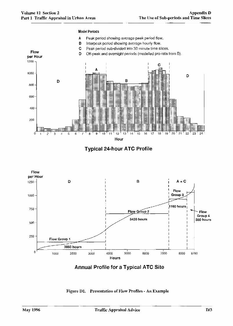
Volume 12 Section 2 Part 1 Traffic Appraisal in Urban Areas
Appendix D The Use of Sub-periods and Time Slices
Model Periods
Flow per Hour
A Peak period showing average peak period flow. B Interpeak period showing average hourly flow. C Peak period sub-divided into 30 minute time slices. D Off-peak and overnight periods (modelled pro-rata from B).
1200
600
Hour
Typical 24-hour ATC Profile
Flow per Hour
1250
1000
500
250
B
- 4.
3420 hours I I - I I
I I
I I
I I I
Flow Group 1 I I I I I I I I I
I---- 3860 hours I I I I I
- Flow Group 4
380 hours
J 0'
I 1000 2000 3000 4000 5000 6000 7000 8000 8760
Hours
D
Annual Profile for a Typical ATC Site
l Figure Dl. Presentation of Flow Profiles - An Example
May 1996 Traffic Appraisal Advice D/3

Appendix D The Use of Sub-periods and Time Slices
Volume 12 Section 2 Part 1 Traffic Appraisal in Urban Areas
Build Peak Period Matrix (usually 2 or 3 hours)
Build Sub Period Trip Matrices & (each at least one hour) %g:;: “;;;;;’
Traffic Count Data
Traffic Flow Profiles for Each Time Slice within Time (Sub) Period
Factor Peak Period
Assign Matrix zra:! .>a ;
for Each Time Slice $ ;, *:
.::::::::,:,, --:i<ii,i.., ,,,:,:,:,,,::::::::., ;;;;; . . ..ii.fi< ,,,,,,,,::,:::: .A.,., :: // p.:::,:: i,,,,,,,,,,,,, : ,,>>xT>““:::;,:w ,.,.,. . . . . . . ..</...., ,, ,,. ,?,...M:::::::::>:,
Factor Sub-Period Matrices to Flow Levels
in Each Time Slice
Figure D2. Derivation of Time Slice Data
‘, Factor Sub-Period “, Matrix to One Hour
: :i ,, : : : : : : : : : : :
Assign One :::::: :::::: Hour Matrix
:::::: ““‘: :‘, :::::/ ,,,,,,
‘:::“iiiiiili::,:iliiiiiiiiiiii ,,I j, ,,, ,,,,,,,,,,,, :::::: ::;:/;///// ,,,,: ..,,,,,,, ,,_,,,,,:::,::::::::::,,:::,,,,,,,,,,,,, ,,, ,!
-
D/4 Traffic Appraisal Advice May 1996
Volume 12 Section 2 Part 1 Traffic Appraisal in Urban Areas
Appendix E Speed/flow Relationships
l Appendix E - Speed/Flow Relationships
El
El.1
El.2
a El.3
El .4
0
INTRODUCTION
The Speed/Flow relationships used in COBA have been derived from national research and are considered to be the most appropriate for use in traffic models. Their use in modelling and economic evaluation of schemes in urban areas helps ensure the compatibility between the economic assessment of different schemes. The standard formulae use nationally-derived relationships to predict the traffic speed associated with a given traffic flow, fitted by local parameters and validated by journey time runs.
Traflc assignment mod& in congested areas usually make use of estimates of delays at junctions in determining route choice, but should be complemented by the use of the COBA relationships on links between the specifically modelled junctions. This Appendix gives details of the relationships for all categories of road and concludes with advice on modelling high speed merges.
The basic form of the speed/flow relationships varies between road classes. For rural, suburban and small town roads the speed of vehicles reduces as flow increases until a critical “break point” flow level is reached, at which the rate of speed reduction becomes greater until capacity is reached. The relationships for urban roads are simpler and they have a uniform speed/flow slope for all flow levels above their nominal capacity. In all cases a flag is set in COBA and a warning message is printed when forecast flow appears to exceed capacity. The same relationships are used within NESA, extended to cover a wider range of road categories to reflect the range of trunk road standards in Scotland.
The standard road classes are as follows:-
Road Class Description for more details:-
1 Rural single carriageway see subsection E2 2 Rural all-purpose dual 2-lane carriageway 3 Rural all-purpose dual 3 or more lane carriageway ;
4 Motorway, dual 2-lanes 1 see subsection E3 5 Motorway, dual 3-lanes 6 Motorway, dual 4 or more lanes 1
7 Urban, non-central 8 Urban, central i see subsection E4
9 Small town see subsection E5 10 Suburban single carriageway 11 Suburban dual carriageway see subsection E6
Table El .I: COBA Road Classes
Classes 1 to 6 are used for all-purpose roads and motorways that are generally not subject to a local speed limit. Their relationships do not allow for speed/flow effects at major junctions. Classes 7 and 8 are used for roads (including junctions) in large towns or conurbations subject to 30 mph (48 kph) speed limits only. Class 9 is used in small towns or villages (excluding junctions) for routes subject to a 30 mph (48 kph) or 40 mph (64 kph) speed limit. Classes 10 and 11 are used for major suburban routes (including some junctions) in towns and cities that are generally subject to a 40 mph (64 kph) speed limit.
May 1996 Traffic Appraisal Advice E/l
Appendix E Speed/flow Relationships
Volume 12 Section 2 Part 1 Traffic Appraisal in Urban Areas
El.5
El.6
El.7
El.8
E2
E2.1
E2.2
E2.3
E2.4
Separate modelling by vehicle class can be important in modelling tFafic route@ in some urban areas. In other areas it can be important for economic assessment and in justifying differential capacities in the peak and contra-peak directions. In these cases the most appropriate speed/flow relationships should be used for each vehicle class.
The relationships can predict speeds above the legal speed limit for the particular road class considered. If this occurs the realism of the predicted speed should be examined and the speed of the relevant vehicle type reduced to the legal speed limit before any economic calculations are made.
Away from the area of immediate interest (ie where flows are not expected to change markedly as a result of the scheme) the use of area wide urban (class 7 or 8) speed/flow relationships, which include an allowance for junction delays, may be satisfactory. The suburban speed relationships (classes 10 & 11) may also prove satisfactory, where the speed limit is 40 mph (64 kph). They too provide estimates of the average journey speed including delays at uncongested junctions.
Within COBA all relationships are subject to a minimum speed cut-off which varies by road class to reflect the likely rerouteing etc which would occur in practice as speeds drop. When speed/$0 w re&iorzshr>s are uxed for truflc modelling purposes, a more direct approach to modelling high flow condition. involvilrg specific modelling of congestion, retiming and rerouteing will need to be adopted. Hence, the use of speed cut-ogs ought not to be necessary. However if a tFaflc model predicts unrealish? speeds adjrtshents must be made to the underlying traflc model - as it is unacceptable to use cut-ofls in URECA interfaces OF to carry forward nnrealtitic speeds to a URECA application.
RURAL SINGLE CARRIAGEWAYS (ROAD CLASS 1)
The rural single carriageway speed/flow relationships apply to single carriageways which do not lose priority, nor are subject to a local speed limit. Table E2.1 defines the geometric parameters and variables used in the relationships and gives the ranges of typical values over which the relationships should apply. The relationships cannot necessarily be taken to apply outside the given ranges of the variables.
Vehicle speeds for a given jlow level are paFticularly dependent on the geomelric variables (CWID, BEND, HILL and HJ. The value of those variables should be calculated, and the rehxtioilships set out in paragraphs E2.6 & E2.7 applied, for at least each individual road link on which flows change us a result of the scheme beina evahrated. For other links, similar roads may be allocated to one of a number of typical link types (eg 6.7m bendy) each representing averaged characteristics. The use of a single road type for roads with markedly different characteristics (particularly free flow speeds) should be avoided.
The actual width of surfaced road is defined by two parameters. The first (CWID) being the width of carriageway between any continuous white lines which may or may not be delineating a hard strip. The second (SWID) is the total width of any continuous edge line and hard strip, which increases the effective carriageway width as set out in para E2.7 by at least 0.8 metres and thus increases free flow speeds as well.
The COBA manual shows how measurements of bendiness, hilliness and visibility are taken. Hilliness is (H, + Hr) and net gradient NG is (H, - Hr). On two-way links net gradient is always zero because the two directions of flow are not disaggregated. On one-way links, rises and falls are defined with respect to the direction of traffic flow; in general they will not cancel out.
El2 Trafic Appraisal Advice May 1996
Volume 12 Section 2 Part 1 Traffic Appraisal in Urban Areas
Appendix E Speed/flow Relationships
E2.5 The average sight distance VISI is the harmonic mean of individual observations. For proposed new roads, VISI should be calculated as set out in the COBA manual from engineering drawings. For existing roads, an empirical relationship has been derived which provides estimates of VISI given bendiness and edge details :
Log VISI = 2.46 + (VWID + SWID)/25 - BEND/400.
This relationship should normally be used for all existing roads for which bendiness and verge width have been measured. On long straight roads or where sight distance is available outside the highway boundary, VISI should be set to 700 metres for roads with high visibility; otherwise estimates should be made from plans or site measurements.
SYMBOL VARIABLE DESCRIPTION TYPICAL VALUES Min Mm
DES Is road designed to TD9/81 (DMRB 6.1.1.) Standards? Yes or No
BEND Bendiness; total change of direction (deg/km) 0 150
HILLS Hilliness; total rise (H,) and fall (H,) (m/km) 0 45
NG Net gradient one-way links only (m/km) -45 45
JUNC Side roads intersection, both direction (no/km) 0 5
CWID Average carriageway width between white line edge 6 11 markings, excluding any painted out portion (m)
SWID Average width of hard strip on both sides, including width of 0 1.0 white line (m)
VWID Average verge width, both sides (m) 0 7
VISI Average sight distance (m) 100 550
PHV Percentage of heavy vehicles (OGVl + OGV2 + PSV) 2 30
VL, VH Speed of light and heavy vehicles (kph) 45 90
SL. &l Speed/flow slope of light and heavy vehicles (kph reduction 5 50 per 1000 increase in Q)
Q Flow all vehicles (vehs/hour/dir)
QJ3 Breakpoint: the value of Q at which the speed/flow slope of 0.8 Qc light vehicles changes (vehs/hour/dir)
QC Capacity: defined as the maximum realistic value of Q (vehs/hour/dir)
900 1600
Table E2.1: Definition of Variables Used in Speed Prediction Formulae for Rural Single Carriageways
May 1996 Traffic Appraisal Advice E/3
Appendix E Speed/flow Relationships
Volume 12 Section 2 Part 1 Traffic Appraisal in Urban Areas
E2.6 The capacity of a single carriageway per direction is:
Qc = 2400(CWID - 3.65)/CWID x (92 - PHV)/80 vehs/hour.
This value of QC ident@7es links which are likely to be overloaded. Whets Jo ws reach this level the user must decide whether the flows are real&ic and what course of action to take.
The point of change of slope (Q,) is given by the relationship:
Qa = 0.8 QC.
E2.7 For flow levels less than the breakpoint QB the speed prediction formulae for light vehicles in kph is:
V, = 72.1 - 0.09 x BEND or -0.015 x BEND for roads designed to TD9/81
- 0.0007 x BEND x HILLS
- 0.11 x NG (one-way links only)
- 1.9x JUNC
+ 2.0 x CWID
+ SWID (1.6/SWID + 1.1)
+ 0.3 x VWID
+ 0.005 x VISI
- (0.015 + (0.00027 x PHV)) x Q.
NOTE: for two-way links HILLS is the average of H, + H,; for one-way links HILLS is H, alone.
E2.8 For flow values greater than Qs the speed prediction formula for light vehicles is:
v, = \lB - 0.05 x (Q - QJ,
where V, = speed at Q = QEl.
E2.9 For all flow levels the speed prediction formula for heavy vehicles in kph is:
V, = 78.2 - 0.1 x BEND or ZERO for roads designed to TD9/81
- 0.07 x HILLS
- 0.13 x NG (one-way links only)
- 1.1 x JUNC
+ 0.007 x VISI
+ 0.3 x VWID
- 0.0052 x Q,
subject to the constraint that if the calculated value of V, is greater than V, then V, is set equal to V,+, which is often the case in non-hilly areas.
E2.10 Within traflc models and URECA applications speed cut-qfls ought not to be necessary. However, it in good prach’ce to compare lheir model outputs against the minimum speed cut-opused by COBA for
the same road type. In the case of rural single carriageways the COBA cut-off is 45 kph. Hence, particular attention should be given to the realism of any traffic model which predicts speeds lower than this on rural single carriageways, (after averaging speeds for very short links with their neighbours).
E2.11 The speed prediction formulae should be used to estimate speeds in the two directions of travel separately on important links where there are significant differences in net gradient or sight distances.
El4 Traffic Appraisal Advice May 1996
Volume 12 Section 2 Part 1 Traffic Appraisal in Urban Areas
Appendix E Speed/flow Relationships
a E3 RURAL ALL-PURPOSE DUAL CARRIAGEWAYS AND MOTORWAYS (ROAD CLASSES 2-6)
E3.1 The speed/flow relationships apply to dual carriageways and motorways which do not lose nrioritv. nor are subiect to a local speed limit. Table E3.1 below defines the variables used in the relationships and gives the ranges of values over which the relationships should apply. The relationships cannot necessarily be taken to apply outside the given ranges of the variables.
SYMBOL VARIABLE DESCRIPTION
BEND Bendiness; total change of direction (deg/km)
HILL Sum of rises and falls per unit distance (m/km)
HII Sum of rises per unit distance one-way links only (m/km)
HF Sum of falls per unit distance one-way links only (m/km)
PHV Percentage of heavy vehicles (OGVl + OGV2 + PSV)
VL, VII Speed of light and heavy vehicles (kph)
%. SH Speed/flow slope of light and heavy vehicles (kph reduction per 1000 increase in Q)
Q Flow, all vehicles, two-way or one-way (vehslhourllane)
QB Breakpoint: the value of Q at which the speed/flow slope of light vehicles changes (vehs/hour/lane)
V, Speed of vehicles at flow Qt, (kph)
QC Capacity: defined as the maximum realistic value of Q (vehs/hour/lane)
TYPICAL VALUES Min Ma:
0 60
0 45
0 45
0 45
2 30
45 speet limit
0 55
0 2300
1080 or 1200
80 105
1400 2250
Table E3.1: Definition of Variables Used in Speed Prediction Formulae for Rural All-Purpose Dual Carriageways and Motorways
E3.2 Vehicle speeds for a given jlow level are particularly dependent on the geomettic vatibles (BEND, HILL and HJ. The value of those variables should be calculated, and the relatiolzships set out in paragraphs E3.5 & E3.6 applied, for at least each individual road link on which flows chance us a result of the scheme beinp evaluated. For other links, similar roads may be allocated to one of a number of typical link types (eg D3L uphill) each representing averaged characteristics. The use of a single road type for roads with markedly different characteristics (particularly free flow speeds) should be avoided.
E3.3 Qc, the maximum realistic value of Q, per lane is:
2330 / (1 + 0.015 x PHV) for motorways, and 2100 / (1 + 0.015 x PHV) for all-purpose dual carriageways.
May 1996 Traffic Appraisal Advice E/.5
Appendix E Speed/flow Relationships
Volume 12 Section 2 Part 1 Traffic Appraisal in Urban Areas
E3.4
E3.5
E3.6
E3.7
E3.8
E3.9
Q,, the value of Q at which the speed/flow slope changes, is taken as 1200 and 1080 vehicles/hour/lane for motorways and all-purpose dual carriageways respective1.y.
For flow levels less than the breakpoint (QJ the speed prediction formula for light vehicles, in kph is:
v, = KL - 0.1 x BEND - 0.14 x HILL (two-way links only) - 0.28 x H, (one-way links only) -sLxQ,
where KL is 108 for dual 2-lane all-purpose (COBA Class 2) 11.5 for dual 3-lane all-purpose (COBA Class 3) 111 for dual 2-lane motorways (COBA Class 4) 118 for dual 3-lane motorways (COBA Class 5) 118 for dual 4-lane motorways (COBA Class 6),
and S, Ihe speed/flow slope for light vehicles, is 6 kph per 1000 vehicles.
At flow levels greater than the breakpoint (QB) the speed prediction formula for light vehicles, in kph is:
V, = V, - 33(Q - Q,J/lOOO.
There is no allowance for delays at any junctions in the above formzdue. Any such delays shordd be sepurutely modelled as set out in detail in sub-section E7 of thk Appendk
The speed prediction formula for heavy vehicles which is applied at all flow levels, in kph is:
v,., = K,, - 0.1 x BEND - 0.25 x HILLS (two-way links only) - 0.5 x H, (one-way links only),
where K, is 86 for all-purpose 93 for motorways
(COBA Classes 2 and 3) (COBA Classes 4, 5 and 6),
subject to the constraint (which is unlikely to apply before the breakpoint) that if the calculated value of V, is greater than V, then V, is set equal to V,.
Within truflc models and URECA applications speed cut-ofls ought not to be necessary, However, it is good practice to compare their model outputs agaimt the minimum speed cut-of used by COBA for the sume road type. In the case of rural dual carriageways and motorways the COBA cut-off is 45 kph. Hence, particular attention should be given to the realism of any traffic model which predicts speeds lower than this on these classes of road, (after averaging speeds for very short links with their nei,ghbours).
The dual carriageway speed/flow relationships are expressed in flow per lane and not flow per direction as is the case wilh single carriageways. The research to develop the speed/flow relationships was undertaken on links with close to the standard 3.65 metre width lanes and was not able to detect a significant width parameter for use in the speed prediction formulae. Also it found that, unlike single carriageway links, the average speed of light vehicles on al-purpose dual carriageways is not influenced by the presence of a hard strip. However, if the average lane width of the proposed scheme is significantly less than the standard 3.65 metres then it may be necessary to survey free flow speeds and use a local speed/flow relationship.
E/6 Traffic Appraisal Advice May 1996
Volume 12 Section 2 Part 1 Traffic Appraisal in Urban Areas
Appendix E Speed/flow Relationships
EY UREWN ROADS (ROAD CLASSES 7 AND 8)
E4.1 Away from the area of immediate interest (ie where flows are not expected to change markedly as a result of the scheme) the use of area wide class 7 or 8 speed/flow relationships which include an allowance for junction delays may be satisfactory. These apply to that part of the main road network in towns (population greater than 70,000) and cities where there is a 30 mph (48 kph) speed limit. They are linear relationships of fixed negative slope with a minimum speed cut-off and include an allowance for an average number of junctions.
E4.2 A distinction is made between central non-central areas. Central areas are defined as those including the main shops, offices and central railway stations, with a high density of land use and frequent multi-storey developments, as in the widely used classification ‘central business district’ or CBD. Conurbations will have several CBDs whilst most free-standing towns will normally have only one. Streets which have commercial or industrial development but are not of a high-density CBD nature should not be included in the central area category. Non-central areas comprise the remainder of the urban area. With this classification, the central areas constituted between 4 per cent and 22 per cent (average 11 per cent) of the total street length in the networks of the 13 towns studied.
E4.3 The definition and range of the variables used in the speed prediction formulae are given in Table E4.1.
SYMBOL VARIABLE DESCRIPTION
INT Frequency of major intersections averaged over the main road network (no/km)
TYPICAL VALUES Min Ma:
2 9
DEVEL Percentage of road network with frontage development (%) 50 90
V Average vehicle speed (kph) 15 48
vo Speed at zero flow (kph) 28 48
Q Total flow, all vehicles, per standard lane (vehs/hr/3.65m lane) 0 1200
QC Capacity: defined as the maximum realistic value of Q 800 (vehs/hr/3.65m lane)
Table lZ4.1: Definition of Variables Used in Speed Prediction Formulae for Urban Roads
E4.4 All links in a particular area should have the same value for INT or DEVEL, and therefore the same speed/flow relationship per standard lane. Even then changes in speeds would be predicted on a link-by-link basis, but the free flow speed would be set by reference to the network-average conditions.
E4.5 The average vehicle speed V kph at flow Q vehs/hour/3.65m lane is given by the relationship:
V = V, - 30 x Q HOOO,
where V,, the speed at zero flow, is defined below for Central and Non-central areas. The maximum vehicle speed should be limited to the legal speed limit.
May 1996 Traffic Appraisal Advice E/7

Appendix E Speed/flow Relationships
Volume 12 Section 2 Part 1 Traffic Appraisal in Urban Areas
E4.6 A capacity warning is given in COBA at 800 vehicleslhour/3+65m lane. When flows reach this level the user must decide whether the flows are realistic and what course of action to take.
0 This value is not
affected by the proportion of goods vehicles.
E4.7 Closer to the area where the introduction of the scheme being evaluated is predicted to produce major flow changes in urban areas local journey time surveys should be undertaken to validate the modelling of speeds through the area. Where this validation data suggests that the standard speed/flow relationships are inappropriate then the user is advised to use observed values of speed (Vj, and corresponding flow (Qj) through which a line of fixed negative slope of -30 kph per 1000 vehicles is drawn.
E4.8 For traffic modelling purposes speeds may sometimes reflect an observed average speed in excess of the speed limit, whereas for economic appraisal purposes speeds should always be reduced to the speed limit.
EA.9 Within traflc models and URECA applications speed cut-ofls ought not to be necessary. However, it LT recommended practice to compare their model outputs against the minimum speed cut-oflused by COBA for the same road type. In the case of urban roads COBA imposes the constraint that urban speeds should not fall below the slowest average speeds observed in towns in practice. This minimum speed in COBA is 15 kph for central areas and 25 kph for non-central areas. Particular attention should be given to the realism of any traffic model which predicts speeds lower than this (including junction delays and after averaging speeds for very short links with their neighbours).
a
E4.10 Non-central areas (Road Class 7) are defined as all those areas not included in the central area definition. The average network speed V, in kph at zero flow is given by the relationship:
V, = 64.5 - DEVEL 15 kph,
where DEVEL is defined as the percentage of the non-central road network of the town that has frontage devel.opment, counting business and residential development as 100% and open space as 0%. DEVEL is normally in the range 50-90% with average values about 80%. Within COBA the 25 kph minimum speed cut-off applies to these areas.
E4.11 Central areas (Road Class 8) are defined as those including the mai,n shops, offices and railway stations, with a high density of land use as in the widely used classification ‘central business district’ (CBD) . Streets which have commercial or industrial development but are not of a high density central business district nature should not be included in the central area. The average network speed V, in kph at zero flow is given by the relationship:
V, = 39.5 - 5 x INT I4 kph,
where INT is a measure of the frequency of major intersections averaged over the main road network. INT is calculated by dividing the total number of lengths of road between major intersections in the central area by the total length of main road in the central area. Major intersections will generally be roundabouts or traffic signals, but they may also be uncontrolled junctions where a significant traffic movement loses priority.
E4.12 This network based value is not directly comparable with a route based value used for suburban links. INT should generally be in the range 2 to 9 per km, with an average of about 4.5. A value less than 2 is not appropriate for Central areas; if this occurs part or all of the area classified as ‘Central’ should be re-classified as ‘Non-central’. Within COBA the 15 kph minimum speed cut-off applies to these areas. Particular attention should be given to the realism of any traffic model which predicts speeds lower than this (after averaging speeds for very short links with their neighbours).
E/8 Traffic Appraisal Advice May 1996
Volume 12 Section 2 Part 1 Traffic Appraisal in Urban Areas
Appendix E Speed/flow Relationships
E5 SMALL TOWN ROADS (ROAD CLASS 9)
E5.1
E5.2
E5.3
E5.5
E5.6
The small town speed/flow relationships have been developed for towns with a population of less than 70,000 (where the main urban relationships do not apply) and for villages or short stretches of development. Table E5.1 defines the variables used in the relationships and ranges of typical values.
SYMBOL VARIABLE DEXRIPTION TYPICAL VALUES Min Ma?
DEVEL Percentage of route with frontage (%) 35 90
P30 Percentage of route subject to a 30 mph speed limit 0 100
V Average vehicle speed (kph) 25 64
VB Average vehicle speed at QB 38 57
Q Total flow, all vehicles, per standard lane (vehs/hr/365m lane) 0 1200
QB Breakpoint: the value of Q at which the speed/flow slope 70 changes (vehs/hr/3.65m lane)
Table E5.1: Definition of Variables Used in Speed Prediction Formulae for Small Town Roads
Like the suburban speed/flow relationships (COBA Classes 10 and 11) they do not apply to individual links, they model traffic speeds over the whole of a route that is subject to a sseed limit of 30 or 40 mph. Unlike the suburban relationships, however, they do not distinguish between light and heavy vehicles, and they snecificallv exclude iunction delays; hence junctions where the route loses priority must be modelled separately _
These relationships should not be used for routes with an almost continuous 40 mph limit (ie P30 < lo%), or less than 65% development (ie DEVEL < 65). In such cases, the route should be split into links, as appropriate, and the standard rural relationships should be used instead.
The breakpoint flow QB is taken as 700 veh1hour13.65 metre lane. The maximum realistic flow (QJ assumed by COBA is 1200 veh/hour/3.65 metre lane. If modelled flows reach this level the user must decide whether the flows are realistic and what course of action to take.
The average speed in kph of all vehicles for flows below the breakpoint (QB) is given by:
V = 70 - DEVEL/8 - P30/8 - 12Q/lOOO,
where DEVEL is the percentage of the length of route that has frontage development, counting business and residential development as 100% and open space as 0%: the value will normally lie in the range 35% - 90%.
For flows greater than Q, the average speed in kph of vehicles is given by:
V - V, - 45 (Q - Q&/1000,
Withiu traflc models and URECA application speed cut-ofls ought not to be necessary. However, it is good practice to cornpare their model outpnn~~ against the minimum speed cut-of used by COBA.for the same road type. In the case of small town roads COBA imposes a 30 kph minimum speed cut-off to these areas. Particular attention should be given to the realism of any traffic model which predicts speeds lower than this (after averaging speeds for very short links with their neighbours).
May 1996 Traffic Appraisal Advice El9
Appendix E Speed/flow Relationships
Volume 12 Section 2 Part 1 Traffk Appraisal in Urban Areas
E6 SUBURBAN ROADS (ROAD CLASSES 10 AND 11)
E6.1
E6.2
E6.3
E6.4
The suburban speed relationships apply to the major suburban routes in towns and cities where the speed limit is generally 40 mph (64 kph). They provide estimates of the average journey speed of light and heavy vehicles separately, including delays at junctions. However, congested junctions should be modelled separately and not included in the calculation of the value of INT.
Generally the use of area wide class 10 or 11 speed/flow relationships which include an allowance for junction delays will be satisfactory away from the area of immediate interest.
The basic form of the relationships is that speed reduces as flow increases. The initial speed is dependent upon the road standard, the number of major intersections and the number of minor intersections and private drives. The rate of decrease in speed is dependent upon the number of major intersections until a critical flow is reached at which point the rate of speed decrease changes to a fixed value until a minimum speed cut-off is reached. (see para E6.11)
Table E6.1 below defines the variables used in the relationships and gives the ranges of values over which the relationships apply. The relationships cannot necessarily be taken to apply outside the given ranges of the variables. The geometric variables INT and AXS should be averaged over a reasonable length of link, generally not less than two kilometres.
SYMBOL VARIABLE DESCRIPTION TYPICAL VALUES min mxi
INT Frequency of major intersections (no/km) 0 2
AXS Number of minor intersections and private drives 5 75 (no/km)
PHV Percentage of heavy vehicles (%) 2 20
VIsVki Speed of Light and Heavy Vehicles (kph) 25 64
&SH Speed/flow slope of light and heavy vehicles (kph) 0 45 reduction per 100 increase in Q
vo
Q
Speed at Zero flow (kph)
Total flow, all vehicles, per standard lane (vehs/hour/3.65m lane)
48 64
0 1500
QB Breakpoint: the value of Q at which the speed/flow slope changes (vehs/hour/3.65m lane)
1050
QC Capacity: defined as the maximum realistic value of Q (vehs/hour/3.65m lane)
1350 1700
Table E6.1: Definition of Variables Used in Speed Prediction Formulae for Suburban Roads
E/10 Traffic Appraisal Advice May 1996
Volume 12 Section 2 Part 1 Traffic Appraisal in Urban Areas
Appendix E Speed/flow Relationships
0 E6.5 There are important differences between the definition of the variable INT for suburban compared to urban roads. In suburban roads INT is specific to each section of route and classified junctions, whose delays are separately assessed, should be excluded from INT. Major intersections are either roundabouts or traffic signals. Junctions between consecutive links should not be double counted. The number of minor intersections and private drives, AXS, should be the total for both sides of the road (even for dual carriageways).
E6.6 The maximum realistic flow (QC), which triggers the overcapacity flag in COBA is the same for both single and dual carriageways and is calculated by the relationship:
QC = 1500 (92 - PHV)/80 veh/hour/3.65m lane.
When flows reach this level the user must decide if the flows are realistic and the course of action to take.
E6.7 The point of change of slope (QB) of light vehicles by the relationship:
QB = 0.7 x QC = 1050 vehs/hour/3.65m lane.
l E6.8 The speed for vehicles (V,) at zero flow (Q = 0) in kph is given by:
V, = C - 5 x INT - 3 x AXSl20,
where, for single carriageways - ROAD CLASS 10
C = 70 for light vehicles, and C = 64 for heavy vehicles,
for dual carriageways - ROAD CLASS 31
C = 80 for light vehicles, and C = 74 for heavy vehicles.
E6.9 The rate of decrease in speed (S) with increasing flow is the same for light and heavy vehicles and for single and dual carriageways. For values of flow (Q) less than the breakpoint (Q& for light vehicles and for all flow ranges for heavy vehicles:
S, = S, = 12 + 50 x INT/3 kph per 1000 vehicles.
For values of flow (Q, greater than the breakpoint (QB) the speed/flow slope for light vehicles increases to:
S, = 45 kph per 1000 vehicles.
E6.10 The speed/flow slope for heavy vehicles does not increase when flow levels exceed the breakpoint. Therefore the calculated speed of heavy vehicles can exceed the speed of light vehicles, when this occurs the speed of heavy vehicles (V,) must be set to the speed of light vehicles (V,).
E6.11 Within tra$j% modeIs and URECA applications speed cut-offs ought not to be necessary. However, it is good practice to compare their model ontpufs against the minimum speed cut-offused by COBA for the same road type. In the case of suburban roads COBA employs minimum speed cut-offs of 25 kph for single carriageways and 35 kph for dual carriageways and maximum speeds limited by the legal speed limit. Particular attention should be given to the realism of any traffic model which predicts speeds higher than the speed limit or lower than the speed cut-offs (after averaging speeds for very short links with their neighbours).
May 1996 Traffic Appraisal Advice E/11
Appendix E Speed/flow Relationships
Volume 12 Section 2 Part 1 Traffic Appraisal in Urban Areas
E7 MERGE MODELLING ON HIGH SPEED ROADS
E7.1 Research by TRL into traffic behaviour on high speed roads (published in CR 279) has allowed the speed/flow relationships incorporated in COBA 9 to be updated. Further research then developed a modified speed/flow relationship on the links between junctions (already described in paragraph E3.6) and a relationship for the delay caused by merges on high speed roads. The resultant advice on merge delays applies to all merge types (including lane gains) which involve weaving and merging manoeuvres.
E7.2 The merge dehy formula ti:-
Dehy = 227 (downstream jlo w/averuge capacity - 0.75) seconds per vehicle.
Thh Ls applicable when flows exceed 0.75 times average capacity and increases linearly with flow. WheJz flows reach average capacity delay per vehicle is 57seconds. It applies equally to ull traflc when acceleration lanes are provided to Departmental design standards (80 kph or higher), as then traffic can merge with minimal delay at that point. The extra traffic joining at such merges reduces gap lengths in the downstream traffic flow until the traffic is able to spread out. However, when flows are heavy, average capacity may be exceeded and “flow breakdown” may follow starting 0.5 to 2 kilometres downstream from the merge point, rather than from the merge point itself. After flow breukdown, capacity B reduced by 5-10s and speeds are s&n@cantly reduced. Average capacity reflects situations both with and withoutflow breakdown.
E7.3 Behaviour at such merges is therefore different from the “Give Way” mechanism, usually based on a gap acceptance, which forms the underlying basis of most congested assignment packages. The mechanism of demand exceeding capacity can be represented in most congested assignment packages by means of their “blocking back” procedures. These use a mechanistic process which at some point usually reduces effective capacity on upstream links and can thus propagate blocked backed queues onto either a) the upstream link designated as giving way, or b) predominantly onto the more congested upstream link (which can be either the mainline or joining feeder), where priorities are designated as equal.
E7.4 There is no evidence to support either apriori rule at High Speed Merges. Hence, unless evidence has been collected over 10 or more days which shows that a more appropriate factor can be calibrated locally, blocking back in truflc models of high speed merges should be controlled by the analyst to delay ‘joining ” and “mainline ” truflc to an equal extent. This can be achieved by keeping the modelled blocking back delay downstream of the merge. This may require careful choice of the model parameter for the average length of a vehicle in a queue, or other measures of stacking capacity. For example at least 15% overcapacity can be handled on a 2km link length by using 5.75m per vehicle (which is in practice less than that observed on High Speed Roads).
E7.5 Thus the recommended procedure is to model high speed merges on a “No Priority” basis with a downstream link length of 2 km &less merges are more closely spaced than that) and check where blocking back is forecast to occur. If any blocking back is forecast upstream of the merge considtr reducing the purumeter representing the average length of a vehicle in a queue for that link. The number of modelled blocked back vehicles should be monitored and the potential for their interaction with other traffic movements which do not pass through the merge considered. Alternative procedures could then be justified and may be required where such interactions already occur.
E7.6 Such modelling needs to be complemented by the icse of a speciul node type at the downstream end qf the Link to simulate the additional merge delay. Alternatively the link may be given a special speed/flow relationship, which mimics standard speed/flow effects up to the breakpoint (1,200 vehs/hour/lane or 1,080 on all purpose roads) and introduces the additional merge delays as per paragraph E7.2. The slope of such a relationship will be dependent on the length of the link and will vary significantly for different percentages of HGV.
E/12 Traffic Appraisal Advice May 1996
Volume 12 Section 2 Part 1 Traffic Appraisal in Urban Areas
Appendix F The Application of Peak Spreading
Fl
Fl.1
F1.2
0
F1.3
F1.4
F2
F2.1
a
F2.2
0
Appendix F - The Application of Peak Spreading
DEFINITION
The term ‘peak spreading’ refers to a reduction in the proportion (though not usually the absolute quantity) of traffic in the most congested part of the peak period, with corresponding increases immediately before and after the height of the peak. This phenomenon falls into two basic categories: ‘passive’ peak spreading (which involves journeys extending beyond the intended part of the peak because of increased delays and is increasingly modelled by passing information on queuing vehicles between time slices), and ‘active’ peak spreading (which involves people starting their journeys earlier or later to avoid the worst traffic conditions or starting earlier so as to arrive at their destination at the same time zs previously).
The opposite effect (‘peak contraction’), can also be an important consideration for schemes that result in significant reductions in travel time over a wide area. In practice, all types of peak spreading occur naturally as traffic demand increases, and without careful analysis can be difficult to distinguish from each other and from other causes of differential growth in peak and off peak travel.
Any modelling of peak spreading, or peak contraction, necessarily will be a simplification of a complex behavioural response to changes in congestion and other factors. None of the methods described in this Appendix is wholly satisfactory. The methods represent the results of interim research pending fuller research into appropriate ways of incorporating peak spreading into traffic models. Further advice on this subject will be issued in due course.
Active peak spreading is less prevalent in the PM peak period, than in the AM peak period, and passive peak spreading is correspondingly greater. In the absence of local data a weaker relationship or no PM peak spreading should be assumed.
APPLICATION TO TRAFFIC MODELLING
Congested assignment techniques using time slicing and information on inherited queues and delays attempt to model ‘passive’ peak spreading effects and ‘passive’ peak contraction. ‘Active’ or combined peak spreading (or contraction) can also be modelled by adjusting the proportion of the peak period traffic demand that is allocated to each time slice. This could be an automated process within for example the mechanism for dealing with inherited queues, or by means of manual intervention by the analyst. Since levels of congestion are usually different in different parts of an urban area, and this leads to differential peak spreading effects, such adjustment methods should preferably avoid uniform factoring.
Several methods for incorporating the effects of peak spreading into urban traffic models have been identified. One has been used by StebbinEs at the Greater Manchester Transportation Unit (GMTU), and is described in References Fl, F2 and F.5. It involves creating and applying the following uniform relationships between the proportion (PH/PP) of peak period traffic that occurs in the peak hour, and an index of peak period traffic growth. The duration of the peak periods used is 3 hours in each case.
PH/PP = 0.514 -0.0846 G (where G = daily traffic growth factor - since 1980) PH/PP = 0.588 -0.1555 G (where G = peak period traffic growrh factor - since 1982) PH/PP = 0.606 -0.189 G (where G = peak period traffic growth factor - since 1984)
The resulting relationships are not suitable for application outside Greater Manchester, and local relationships must be calibrated from past count data if the method is to be applied in other areas. In the
May 1996 Traffic Appraisal Advice F/l
Appendix F The Application of Peak Spreading
Volume 12 Section 2 Part 1 Traffic Appraisal in Urban Areas
F2.3
F2.4
F2.5
F2.6
F2.7
same way, the assumption of linearity is not binding for all applications. Although there is no theoretical basis for this, the relationship calibrated from historic data is normally extrapolated into the future, and care must be taken to ensure that this gives sensible results for future years.
Hounsell has also carried out a study for the TRL into the incorporation of peak spreading into congested assignment models (Reference F3). This explored two methods of adjusting traffic demand profiles to reflect peak spreading. The first was that used by GMTU, and described above. The second involved the identification of past traffic growth trends in short periods within the peak period, relative to growth in the peak period as a whole. This method suffers from the same drawback as the GMTU approach, that trends in the past are assumed to be applicable to the future, and that relationships are not necessarily transferable between study areas.
Goodwin & Coomhe when at Halcrow Fox developed a relationship that they saw as suitable for general application, based on data from a number of towns and cities with different existing levels of congestion (London, Bristol, Birmingham, Bournemouth, Exeter, Norwich, Ipswich and Bury St Edmunds) _ It takes the following form:
R = 1 - k.vZ
where R is the ratio of the flows in the two half-hour periods adjacent to the peak hour to the flow in the peak hour itself - the ‘peakiness factor’;
and
V is the average peak hour traffic speed (kph);
k is a calibrated coefficient specific to the chosen peak period (0.0001935 for AM or 0.0001089 for PM).
The average peak hour traffic speed relates to the modelled network as a whole, and flow variations were derived from appropriate traffic surveys. The method is applied iteratively, with speeds from successive assignments being used to recalculate the value of the ‘peakiness’ factor and, hence, to revise the trip matrices input to the assignment. Further details are given in Reference F4.
This method assumes that each peak period has a fixed length of 2 hours, so that the relationships involved would have to be re-calibrated to accommodate longer or shorter peak periods. A further disadvantage is that it only gives information about the scale of peak hour demand in relation to the peak period as a whole, and no information is available about the allocation of trips to the preceding and following half hours. This method is sensitive to reductions in congestion, and is therefore capable of representing ‘peak contraction’ effects.
Three other still experimental approaches are deemed to be more suitable for modelling changes in peak profiles in Reference FS and those and other ideas are described below.
Count Based Models: These techniques estimate a functional relationship between the peak hour to peak period ratio (PH/PP) and explanatory variables for congestion in the network, using local count data. They employ a negative exponential form, with the peak hour volume to capacity ratio (V/C) as explanatory variable. For a three-hour peak period this would be of the following shape:
PH/PP = 0.333 + A e-bcv’c’
where PH/PP = VIC =
A,b =
peak hour to peak period proportion peak hour volume to capacity ratio on the link,
or flow-weighted on the screenline model parameters
F/2 Traffic Appraisal Advice May 1996
Volume 12 Section 2 Part 1 Traffic Appraisal in Urban Areas
Appendix F The Application of Peak Spreading
l F2.8
F2.9
a
F2.10
F2.11
a F2.12
The model needs to be calibrated using regression techniques on long term data from local sites which are representative of the scheme under consideration. The model needs to be applied to data from the main congestion pinchpoint, whose local V/C ratio is the appropriate determinant for peak spreading. If diversionary routes are available a weighted V/C ratio may be the appropriate determinant. If there are other upstream or downstream bottlenecks, the effect of any forecast capacity improvement may need to be constrained accordingly. In the absence of long term local data, an average slope model can be estimated as follows:
PH/PP = 0.333 + A e-3W’c)
The local intercept parameter A can be estimated from the working day average for PH/PP ratio and peak hour V/C ratio in the base year, as calculated from the ATC data. (This average slope model uses the value for the slope b based on an assessment of observed peak spreading in the morning peak at 38 motorway and trunk road sites in the UK between 1981 and 1991, as described in Reference F6). Clearly, the accuracy of the model will improve with local and longer count data availability.
This approach provides information about the reduction in demand in the busiest hour, but not about the shoulder to which this traffic transfers; the simplest assumption would be a 3 to 1 transfer to pre- and post-peak. Alternative proportions designed to counteract the modelled passive peak spreading, or from local historic count data may indicate however a more appropriate split.
Proportionate Models: These use Stated Preference or other techniques to determine the proportion of drivers who when faced with a pre-specified level of congestion would set off earlier, rather than later and builds a utility function incorporating such a mechanism. Research into this approach is still being undertaken. In the interim it may be possible to modify the process of queuing vehicles being passed between time slices, within existing traffic modelling packages by using Origin-Destination data on those vehicles, estimated proportions moving earlier and an iterative process.
Multi-Period EIouilibtium Models; These aim to maintain relative travel times (or generalised costs) between time periods, once they exceed a pre-determined limit. Flows in each time period are modelled simultaneously and calibrated penalties introduced representing drivers’ reluctance to shift from the desired to an earlier or later period with less congestion. Calibration is based on historic data covering a number of years during which drivers were known to time shift. Multi-period equilibrium models are not unlike shadow networks and employ standard equilibrium assignment techniques on extended networks, in which the extensions in this case represent alternative departure time choices.
The multi-period equilibrium approach is most suitable in complex networks, where more than a single bottleneck affects travel times on routes, and where different OD-pairs are affected in different ways by either the increase in congestion or the impacts of a road scheme. The approach works as follows:
run a multi-period base year assignment with the base year profile; determine the matrix of trips modelled as spreading away from the peak hour; transfer a similar matrix from the shoulders back to the peak; re-run the multi-period assignment with the new desire matrix and check whether the observed base profile is reproduced; repeat the procedure until assignment of desire profile leads to observed base profile.
Through this trial-and-error approach the desire profiles should be determined, expressing the distribution of travel demand over the constituent time periods in the absence of congestion. These desire profiles are likely to vary by trip purpose and are a function of the modelled transfer penalties per purpose. Once the desire profiles have been established the model can be used in a forecasting mode.
May 1996 Traffic Appraisal Advice F/3

Appendix F The Application of Peak Spreading
Volume 12 Section 2 Part 1 Traftic Appraisal in Urban Areas
F2.13
F2.14
F2.15
F2.16
F2.17
Incremental Logit Models of Denarture Time Choice: The concept behind incremental logit models is similar to the multi-period equilibrium technique: changes in travel costs per time peri,od are assumed to govern the spread of demand over the peak period. Full details are given in reference F7.
An observed base year peak profile is taken and after assignment gives rise to reference costs per OD-pair in each time period. Using forecast growth in the peak period as a whole “no-change demand flows” in each of the constituent peak hours are calculated for the target years. An assignment of these no-change demand flows produces target year “no-change costs” per OD-pair per time period.
The incremental logit model then estimates a new peak profile, based on the “no-change profile” of trips in the target year, and the change in costs in each time period between reference and target years. The basic form of the incremental logit model is:
where P, = proportion of trips in time period t in the target year St = no-change trips for ti,me period t in the target year Ct = costs in time period t in the target year dt = costs in time period t in the reference year 13 = local sensitivity parameter
The costs used in the incremental logit model should be OD-specific costs.
A model based on cost ratios is also possible. Whereas the model based on absolute cost differences would tend to shift long-distance trips first, the model based on cost ratios places a greater emphasis on short distance travel:
The sensitivity parameters p play a vital role in these incremental logit models. They should be estimated locally, by calibrating the logit model using a trial and error approach to the estimation of /I using count data at least 3 years apart. Sensitivity testing with respect to model parameters is advisable.
References Fl
F2
F3
F4
F5
F6
F7
Stebbings F. Forecasting Peak Spreading. GMTU Note 52. July 1988.
Stebbings F. Further Peak Spreading. GMTU Note 234. May 1993.
Hounsell N.B. Peak Spreading and Congestion: Some Preliminary Analysis. Transport and Road Research Laboratory. Contractor Report 268. 1991.
Goodwin R.P. and Coombe R.D. _ Dealing with the National Road Traffic Forecasts in Urban Areas. PTRC 19th Summer Annual Meeting, Seminar G. 1991.
Van Vuren T. Porter S.J. & Sharpe M.A. Advice on modelling changes in peak profiles for road scheme appraisal. PTRC 23rd European Transport Forum, Seminar F. 1995.
Porter S.J, Field M.A. and Van Vuren T. Evidence of Peak Spreading in the UK. PIRC 23rd European Transport Forum, Seminar F. 1995.
Chin KK, Van Vliet D. and Van Vuren T. An equilibrium model of departure time and route choice. PTRC 23rd European Transport Forum, Seminar F. 1995.
F/4 Traffic Appraisal Advice May 1996
Volume 12 Section 2 Part 1 Traffic Appraisal in Urban Areas
Appendix G Growth Constraint Tcchniqucs
Appendix G - Growth Constraint Techniques
Gl INTRODUCTION
Gl. 1 Growth constraint techniques are required where unconstrained growth, or growth constrained at a strategic level by a higher tier model, would result in the model predicting unrealistic local traffic conditions, e.g. numerous instances of severe delays, the appearance of grid-lock and/or unrealistic routeing. In general, the network will need to be examined at three levels of detail to assess the onset of saturation:
0 at the network level, queues may build up steadily through the modelled period without being cleared at the end of the period;
0 at a sector level, overall zone to zone speeds may fall below a critical level for a significant number of origin to destination pairs; and
0 at a local level, pockets of severe congestion may arise where vehicles are effectively stationary for significant periods of time.
01.2 Several different methods have emerged in the past few years for constraining growth in traffic models used for highway scheme appraisal. These fall into the following categories:
0 user-determined factors or cut-offs;
0 matrix capping techniques;
0 elasticity techniques;
0 incremental loading techniques; and
0 shadow network techniques.
Gl f 3 Each of these methods tends to concentrate on one of the aspects of constraint listed in Paragraph Gl . 1, and the method chosen for a particular study will depend to a certain extent on the emphasis required. They can be used (within their limitations) to model Suppressed Traffic and its release in accordance with the Guidance on Induced Traffic issued by the Department in response to the 1994 SACTRA report ‘Trunk Roads and the Generation of Traffic’. However, elasticity techniques are the only ones capable of modelling Induced Traffic in excess of the reference case. A brief description of each type of method is given below and a comparison of several methods is given in Reference Gl.
G1.4 It should be noted that most of the methods rely heavily on the quality of the assignment model and its principal outputs. The assignment model used must therefore be converged, responsive to congestion and based on reliable parameters to give a realistic representation of the traffic conditions that would arise from a given set of travel demands and network characteristics.
G1.5 To avoid the known limitations of these methods, it is recommended that the local realism of any growth restraint techniques used be demonstrated and their local use thus justified. As discussed in Paragraph 5.7.4 in the main body of this report, growth constraint techniques are only a proxy for more complex influences on future travel patterns. The principles set out in Paragraph 5.7.5 should be adhered to. The simplest realistic method should be chosen and implemented with care.
May 1996 Traffic Appraisal Advice G/l
Appendix G Growth Constraint Techniques
Volume 12 Section 2 Part 1 Traffic Appraisal in Urban Areas
G2 USER-DETERMINED FACTORS OR CUT-OFFS
G2.1 User determined factors or cut-offs, based on a comparison of forecast traffic flows and capacities at critical locations on the scheme network (or, less commonly, forecast speeds), are the simplest way of modelling constraints to traffic growth. For simple schemes, where the constraint is approximately the same for all origin to destination movements, it may be possible to apply a single (uniform) factor to each forecast year trip matrix. For more complex schemes, with a wider area of influence, different factors may be applied to different parts of the trip matrix (eg radial, orbital), or model area (urban, suburban, rural, etc.), or may be derived by examining the capacity constraints across natural barriers such as rivers and railways _
G2.2 These methods can handle trip suppression, but trips cannot be generated above those in the original demand matrix and as a result the methods cannot predict the full response to the improved infrastructure. Most applications are not directly related to travel speeds or network capacity.
G3 MATRIX CAPPING TECHNIQUES
G3.1 With these techniques, the aim is to identify the origin to destination movements that pass through the most congested parts of the network, and to reduce these movements (or their growth) to a level that gives a more realistic degree of congestion. This will usually relate to or exceed the level prevailing in the model base year. By applying this process for a succession of forecast years, a logical pattern of constraint should emerge.
G3.2 Techniques similar to those used in m&x estimation (ME2) may be employed to carry out this process, in this case with network capacities speci,fied in place of target traffic counts (e.g. References G2 and G3). The recommended approach is to input a demand trip matrix, actual capacities and a scale factor to allow the precise degree of saturation to be varied, so that a realistic amount of over-saturation can occur before matrix capping takes place. The effect of queues inherited from earlier parts of the model period (and in appropriate cases the effect of trip retiming) may also need to be input. Hence, some assignment methods attempt to automate this part of this process by allowing flow profiling to be taken into account before matrix capping is applied, so that a more realistic assessment of the true degree of over-saturation in any time slice can be made (e.g. Reference G4). Care must be taken when using such methods that all adjacent junctions are modelled in detail to provide continuity of profiling.
G3.3 All of these techniques must use converged assignments and the same assignment procedures as the main assignment model, and the capacities input must be treated as upper limits to traffic flow, not targets. Some assignment methods recommend ‘warm start’ procedures so that abnormal routeings are not embedded in the initial assigned flows. Such procedures must be adopted for Trunk Road appraisals unless local monitoring of their effect, which have been fully documented, justifies alternative procedures.
G/2 Traffic Appraisal Advice May 1996
Volume 12 Section 2 Part 1 Traffic Appraisal in Urban Areas
Appendix G Growth Constraint Techniques
0 G3.4
G3.5
G3.6
G3.7
The effective degree of oversaturation which drivers are prepared to tolerate should be confirmed, a) by reference to experience in similar areas, b) by comparison of forecast and actual queues in the base year
and c) by applying the chosen capping methodology to the validated base year network and traffic matrix (thus checking that the assumed tolerated capping level is not exceeded in the base year).
The trip matrices output from this process must be inspected to see that no origin to destination movement exhibits unjustifiable negative growth or growth significantly in excess of unconstrained growth forecasts; remedial action must be taken l;funacceptable violations occur. In addition, the realism of the most severe constraint must be critically examined and the aggregate situation over each complete model period, inspected even when a different assignment is being carried out for each time slice within the period.
The main advantage of this technique is that it can be related directly to the capacity of individual links (or junctions) in the network being considered. Its disadvantages are that:
0 there is little behavioural justification for the adjustments made beyond any incorporated in the input matrices (i.e. trips are suppressed regardless of their length, overall travel speed or the availability of alternative transport modes); the puttem of trip suppression must therefore be examined, and a judgement made as to its plausibility and consistency;
0 the identification of Ihe origin to destination movements to be adjusted relies heavily on the routes calculated by the assignment model and the location and density of the capping points; steps must be taken to ensure thut overloading of the network does not lead to unrealrjtic routeing (possibly by considering frequent intermediate years), that capping points form screenlines and that tlze capaci& of short links does not uffect the process;
0 turning movement capacities are easiest to use, but inappropriate as turning proportions usually fluctuate widely over a complete model period; hence, where junctions are the major constraint, their upproach link cupacities after repeated signal oph’mtiation and allowing for likely improvements should be used,
0 the method can handle trip suppression, but trips cannot be generated above those in the original demand matrix; so the metlzod is most approprtite for improvements not expected to@& relieve exxisting or expected congestion,. and
,.
0 as a result of the above cautions, careful (and possibly time-consuming) incremental application of the methodology is therefore required;
The technique is likely to suppress fewer short distance trips compared with other methods.
May 1996 Traffic Appraisal Advice G/3
Appendix G Growth Constraint Techniques
Volume 12 Section 2 Part 1 Traffic Appraisal in Urban Areas
G4 ELSTICITY TECHNIQUFS
G4.1 These techniques involve applying elasticity adjustments to trip matrices to model the effects of changing travel costs relative to a previous equilibrium situation (e.g. the ‘do minimum’ assignment for the current forecast year, or the ‘do minimum’ or ‘do something’ assignment for a previous forecast year).
G4.2 The assumption underlying these techniques is that all behavioural responses can be combined into a single trip rate demand curve, which subsume the underlying complex cross elasticities. Appropriate values for use in generalised cost models are set out in the Guidance on Induced Traffic, suitable for use in a range of circumstances. Implied time elasticities can be calculated for the same formulations and where models have been calibrated as time only assignments, the implied time elasticities should be used. Future editions of the Guidance are expected to report both time and generalised cost elasticities.
G4.3 The techniques have their foundation in the economic basis of travel behaviour, but have the following practical disadvantages:
the results are dependent on the elasticities and elasticity functions used; evidence on suitable elasticity values is limited, but recent research (References G5 and G6) has shown that appropriate values depend on trip purpose, trip length, trip orientation (orbital or radial) and the extent to which travel costs increase (i.e. the elasticities are not constant); ICY, nnd the fact that many existing applications use a single elastici~ value, makes the choice of ehzsticihSes vety difficult (the practice of testing dtrerent elastic@ values until an acceptable result LY achieved is indefensible);
if only part of a trip length is represented in the model network, the elastic adjustments can be distorted; thrj problem can apply to both short trips and external trt@s. Both may represent tri]s with a high proportion of their time on zone connectors. Hence, short hlljs may need to be excludedporn the adj’ustmentprocess and elastici@ adjVustments only applied to external trips after allowing for the journey time and distance outside the modelled network;
the value of the elasticity parameter is the only means by which simple elasticity methods can attempt to reflect the opportunities offered to travel to alternative destinations, or by alternative modes of travel; thus multi class assignment may need to be considered as a way of introducing different elastic@ parameters;
the scale of the elastic adjustments are only indirectly related to .network capacity, so that the intended effect of limiting queues and delays at individual junctions to specific maxhum values cannot be guaranteed; and
elasticity techniques adjust trip rates, usually using traffic eh’isticihes which also reflect trip lengthening effects, hence their principal unconstrained effect is to reduce (or increase) the overall numbers of trips in the matrix - in effect, they imply that the dominant traffic response to congestion is the suppression of trips. For most schemes, rerowteing, retiming, redistribution and change of mode are likely to be the major components of the overall response. However, for approprtite geographical& restricted network, elastic adjustments may provide an adequate proxy for the assessment of local traflc impacts.
G4.4 The application of elasticity techniques can sometimes lead to negative growth in some areas and growth above unconstrained levels in other areas. Specific checks should be made of the resultant forecast growth at a zone to zone level to ensure that such effects are valid (i.e. that they represent sensible trip patterns likely to be brought about by known changes in travel characteristics and/or land use). Controls need to be applied (funacceptable results are obtained.
G/4 Traffic Appraisal Advice May 1996
Volume 12 Section 2 Part 1 Traffic Appraisal in Urban Areas
Appendix G Growth Constraint Techniques
0 G4.5
G4.6
G4.7
G4.8
It is possible to apply these techniques as an iterative combination of an elasticity adjustment to a matrix, followed by an assignment of the adjusted matrix and further recycling of the output costs. However, this method may not converge in some cases, particularly where the elasticity is relatively large. An integrated trip demand/assignment procedure (sometimes referred to as ‘elastic assignment’) may be considered, as theoretically it should have better convergence characteristics (Reference G7). Whichever approach is used, checks are still required to ensure that anomalous effects have not arisen and that growth constraints are within acceptable limits.
Elastic adjustments to individual zone to zone flows can be forecast using alternative mathematical formulae, which embody constant elasticities, elasticities which rise or fall with cost, elasticities which are bounded etc. The Power formulation:-
where T, = T,O * (cjj / cjjo) ’
T, is the forecast number of trips T,’ is the forecast number of trips in the reference case cij is the forecast cost cijo is the cost in the base year or reference case
and B is the elasticity, which is constant for all trips
should normally be used in Trunk Road applications. There may be instances where other forms may have superior properties for the local circumstances, in which case the arguments in favour of the alternative formulation must be clearly presented and rigorously justified.
Other mathematical formulations are available. Some of these have the property of Base Independence. (That is that if situation C is forecast directly from A, then the same answer is produced when B is forecast from A followed by C from B.) The Power formulation has this property, is simple to apply, distance neutral and elasticity parameters are not dependent on the units used.
The semi-log (also known as the Elastic Exponential) formulation is also simple to apply, distance neutral and elasticity parameters are not dependent on the units used. However, as it is not Base Independent, it can only give absolutely consistent results when used in a prescriptive and behaviourally realistic way.
Both of these formulations are likely to have a neutral effect on trip length. Other formulations which suppress fewer short distance trips and more long distance trips are less likely to provide a conservative forecast of Variable Trip Matrix economic benefits. This arises as other formulations are more likely to forecast a greater net release of long distance trips, as a result of a scheme, which are likely to be associated with higher consumer surplus benefits than the release of the same number of short distance trips.
May 1996 Traffic Appraisal. Advice G/5
Appendix G Growth Constraint Techniques
Volume 12 Section 2 Part 1 Traffic Appraisal in Urban Areas
G5 INCWMENTAL LOADING TECHNIQUES
G5.1 Incremental loading techniques involve developing demand matrices for a series of future years, and assigning them consecutively. At each stage, travel speeds are monitored separately for each zone to zone movement, and those that have fall.en below a specified minimum speed (which can vary by trip length) are prevented from growing further, or in some applications reduced by a small percentage. Full unconstrained growth is permitted for all other movements (see Reference G8).
G5.2 The main advantage of this technique is that it has a behavioural basis (i-e it attempts to replicate the likely judgement of travellers rather than the characteristics of individual network links and junctions), and gives a smoother transition between forecast years.
G5.3 The disadvantages are similar to those experienced with elasticity techniques, i.e. :
the quality of the results depends critically on the minimum speeds specified, and more particularly on the rel,ationship between minimum speed and distance travelled (for example, short-distance trips generally accept lower overall speeds than longer-distance trips) ;
there is no general agreement as to what the minimum threshold speeds should be or how they should vary with trip characteristics (the usual assumption is that threshold speeds increase with distance) ;
if only part of a trip length is represented in the model network, overall journey speeds are difficult to define: thus the method should only be upplied after allowing for the journey time and distance outstie the modelled network; a less satisfactory alternative is to avoid adjusting long distance tr@ and to upp& the technique only to trips that are contained who& within the modelled network;
the method does not reflect the opportunities offered to travel to alternative destinations, nor by alternative modes of travel;
since there is no direct relationship with network capacity, achieving specific maximum queue and delay objectives cannot be guaranteed;
for a given zone to zone movement, whilst the growth in trip making will be cut off at the specified threshold speed, lower speeds may follow as congestion caused by the growth of other trip movements continues to increase (hence in some applicutions small reductions in existing trips are allowed); and
the method can handle trip suppression, but trips cannot be generated above those in the original demand matrix; so the method is most appropriate for improvements not expected tofu& relieve existing or expected congesh~on.
G5.4 Negative growth is not usually a problem with this technique, since flow levels will stabilise for parti,culat+ movements, and any reductions are controlled by the analyst. However, the output matrices should still be inspected (usually at the sector level) to see that rea1.M~ results are obtained.
G5.5 The effect on trip length distribution can be controlled by making the minimum acceptable speed dependent on trip length and the choice of a suitable relationship.
G/6 Traffic Appraisal Advice May 1996
Volume 12 Section 2 Part 1 Traffic Appraisal in Urban Areas
Appendix G Growth Constraint Techniques
0 G6 SHADOW NETWORK TECHNIQUES
G6.1 These techniques are in many ways similar to the incremental loading techniques outlined above. Here each network description also contains a ‘shadow’ of the true network. In the most common applications this is identical to the true network, except that speeds are fixed and represent assumed minimum travel speeds. Zone connectors feed directly or via extra nodes onto both networks and there is no other connection between them. Thus, only those trips that can achieve overall zone to zone speeds in excess of the minimum threshold speed are assigned to the true network. Minimum threshold speeds can vary by link, or link type, and shorter trips can be made less susceptible to transfer to the shadow network by including fixed delays on the shadow zone connectors, Although it is theoretically possible to represent the shadow network by a series of zone to zone connectors (‘spider network’), this is generally not possible in practice.
G6.2 The method is also capable of using nested shadow networks, with one level representing other time periods and another the public transport network and including appropriate transfer penalties. However, there is no known experience of its use in this way except as a research tool.
a G6.3 This process is able to produce converged assignments that limit congestion to realistic levels. It is again based on traveller behaviour, rather than the effect of individual congestion points, and can be applied relatively easily using existing software packages and is a process which could be automated.
G6.4 The following disadvantages should be noted, however:
0 the choice of minimum travel speeds is difficult, and they cannot be varied easily for different trip length; however, indirect trip length efsects can be introduced by va+zg the delays on the shadow zone connectors, and thlj should be considered as a means of improving behavioural realism; (a minimu,m speed of 15 kph for all but the shortest tr@s ti sometimes considered appropriate);
0 as with ‘incremental’ methods, overall minimum speeds are difficult to define if only part of a trip length is represented in the model network (again, trips that are not contained wholly within the modelled network should be treated with care); and
0 negative growth can be a major problem with this method; some origin to destination movements can fall dramatically, largely because of interaction with other movements, and multi class assignment (separating the base traffic from the exogenolls growth) may need to be used to overcome the worst of these effects.
0 the method can handle trip suppression, but trips cannot be generated above those in the original demand matrix; so the method 13 most approprtite for improvements not expected to&lly relieve existing or expected congestion.
G6.5 The ‘real’ trip matrix required by economic appraisal procedures such as COBA may be derived by identifying Ihe movements contained in the ‘real’ assignment (eg by cordoning on the ‘real’ zone connectors) _ The results should be inspected closely to ensure that they are sensible for each jbrecast year, and action taken as necessary to adjust minimum travel speeds, etc.
G6.6 Without introducing delays on the shadow zone connectors, the technique suppresses large proportions of short distance trips and virtually no long distance trips.
May 1996 Traffic Appraisal Advice G/7

Appendix G Growth Constraint Techniques
Volume 12 Section 2 Part 1 Traffic Appraisal in Urban Areas
Gl
G2
G3
G4
G5
G6
G7
G8
White C., Emmerson P. and Gordon A. Assignment Based Techniques for Modelling Traffic Growth in Congested Areas. Traffic hgineering and Con&o1 Vol. 36 No. IO. October 1995.
Rogers K. Congested Assignment and Matrix Capping - Constraining the Trip Matrix to Reflect Network Capacity Automatically. GMTU Report 182. October 1991_
Rogers K. Congested Assignment and Matrix Capping - Constraining the Trip Matrix to Reflect Network Capacity. Traffic Engineering and Control Vol. 32 No. 7/8. July/August 1991.
Logic M. and Witte R. Dynamic Assignment Modelling with TRIPS. MVA Systematica. 1990.
Coombe D., Leigh S. and Chua H. The Sources of Benefit from Urban Road Improvements. PTRC Summer Annual Meeting. September 1989.
Brown M.B., Evans R.C., Mackie P.J. and Sheldon R. The Development of Elasticities for a Road Pricing Model. PTRC Summer Annual Meeting. September 1993.
SATlZASY User Guide. W.S. Atkins Planning Consultants/ITS Leeds University. November 1991.
Hounsell N.B. Limits to Traffic Growth in Congested Urban Networks. TRRL Contractor Report 171. 1989.
G/8 Traffic Appraisal Advice May 1996

Volume 12 Section 2 Part 1 Traffic Appraisal in Urban Areas
Appendix H Convergence
l Appendix H - Convergence
HI INTRODUCTION
H1.l Before the results of any traffic assignment are used to influence decisions, the stability (or convergence) of the assignment process and the sensitivity to the generalised cost parameters need to be assessed. This appendix is concerned with the stability (convergence) topic which is less well understood than the sensitivity issue. Non converged and unduly sensitive results do not provide reliable forecasts.
H1.2 For all iterative assignment processes convergence is an issue. In some cases the iterative assignment procedure is mathematically guaranteed to converge, so that after an infinite number of iterations a perfectly stable flow and delay pattern which meets the assignment objective will be reached. However, with most advanced assignment models involving explicit modelling of junctions or other options, convergence is not guaranteed.
- H1.3 For practical purposes convergence in assignment should be considered as a reasonable point in the
iterative process, where returns are diminishing, and where the flows and costs are sufficiently stable and within an acceptable proximity to the assignment objective. Convergence in practice needs to be measured in terms of two desirable properties of the flows and costs cakulakd by the programme:
- stability of the model outcomes between consecutive iterations,
- proximity to the assignment objective, (eg. Wardrop equilibrium),
HI .4 The number of iterations in an assignment will generally depend on network size and level of congestion, but in excess of 100 iterations should not be regarded as unreasonable. This implies in many cases a substantil increase over default values. Network size or computing requirements should not be a limiting factor in ucceptabilig of convergence stmdards.
H1.5 Convergence monitoring is an integral part of congested assignment modelling. It is of particular
0
importance:
a) at the initial stages of base year model calibration,
b) when moving to future year forecasts, and
c) in assessing the accuracy of the final results.
May 1996 Traffk Appraisal Advice H/l
Appendix H Convergence
Volume 12 Section 2 Part 1 Traffic Appraisal in Urban Areas
H2 MODEL CALIBRATION - USE OF CONVERGENCE CRITERIA
H2.1 Convergence of congested assignment models can be monitored using a variety of indicators. These can be classified as follows:
a) global stabiliq indicators, based on comparisons between successive iterations of network-wide values of total journey time, total journey distance, total or average travel costs or average speed.
b) disaggregate stability indicators, based on absolute changes in values of individual link flows, costs or times, origin-destination costs or a combination of these,
c) proximi,ty indicators, reflecting how close the cnrrent flow and cost pattern is to the assignment objective.
H2.2 Stabilitv at global level (e.g. total travel time, costs or dtitance) 13 not su@‘icient for ensuring model convergence. Such measures may hide substantial uncertainty at a lower level, such as in individual linkflows or OD-costs. Even though global stabiliy may provide use@1 inform&on during the iterative process, it should always be accompanied by dkaggregute analyses at link or OD-Level. a
H2.3 Of a large number of disazreEate stability indicators, the following three have been identified as being straightforward to compute, easy to interpret and explain, and robust in their explanation of assignment stability.
a) average absolute difference in link flows between successive iterations:
where : N = number of links Van = flow on link a in iteration n
b) relative average absolute difference in link flows between successive iterations:
N I n-1 -DE+ v:-va I 4-l v,“-’
c) %FLOW, the proportion of links in the overall network with flows changing less than 5% from the previous iteration,
H2.4 Proximitv measures can only be calculated when an asignment objective has been formulated- This is usually the case with equilibrium assignment, and deterministic extensions (multiple user classes, dynamics, elastic assignment). In stochastic assignment (Burrell or Dial) such an objective cannot be defined and convergence can only be measured in terms of stability.
HI2 Traffx Appraisal Advice May 1996
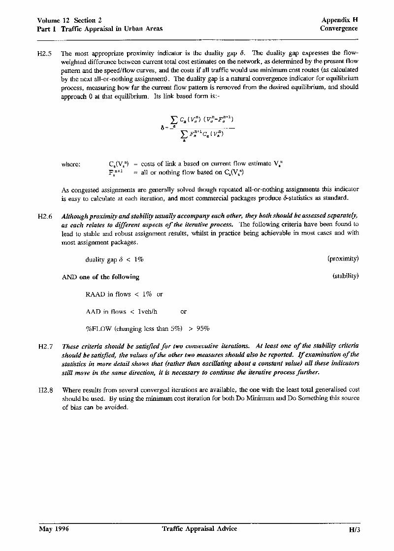
Volume 12 Section 2 Part 1 Traffic Appraisal in Urban Areas
Appendix H Convergence
0 H2.5 The most appropriate proximity indicator is the duality gap S. The duality gap expresses the flow- weighted difference between current total cost estimates on the network, as determined by the present flow pattern and the speed/flow curves, and the costs if all traffic would use minimum cost routes (as calculated by the next all-or-nothing assignment). The duality gap is a natural convergence indicator for equilibrium process, measuring how far the current flow pattern is removed from the desired equilibrium, and should approach 0 at that equilibrium. Its link based form is:-
c c,w:, K-F3 SE 1
c F,“+k, ( v,“, a
where: C,(V,“) = costs of link a based on current flow estimate VP Fan+1 = all or nothing flow based on C,(V,“)
0
As congested assignments are generally solved though repeated all-or-nothing assignments this indicator is easy to calculate at each iteration, and most commercial packages produce a-statistics as standard.
H2.6 Althoughproximity and stability usually accompany each other, they both should be assessed separately, as each ret&es to d@erent aspects of the iterative process. The following criteria have been found to lead to stable and robust assignment results, whilst in practice being achievable in most cases and with most assignment packages.
duality gap S < 1% (proximity)
AND one of the following (stability)
RAAD in flows < 1% or
AAD in flows < lveh/h or
%FLOW (changing less than 5%) > 95%
0 H2.7 These criteria should be satisfied for two consecutive iteratiorts. At least one of the stability criteria
should be satisfied, the values of the other two measures should also be reported. If examination of the statistics in more detail shows that (rather than oscillating about a constant value) all these indicators still move in the same direction, it is necessary to continue the iterative process further.
H2.8 Where results from several converged iterations are available, the one with the least total generalised cost should be used. By using the minimum cost iteration for both Do Minimum and Do Something this source of bias can be avoided.
May 1996 Traffic Appraisal Advice H/3

Appendix H Convergence
Volume 12 Section 2 Part 1 Traffk Appraisal in Urban Areas
H3
H3.1
H3.2
H3.3
H3.4
H3.5
CONVERGENCE MONITORING FOR DIFFERENT ASSIGNMENT METHODS
Not all of the above criteria are applicable to all assignment options:
in user equilibrium assignment both proximity and stability should be satisfied;
in multiple user class assignment stability should be monitored for each class separately; proximity should be assessed for total flow;
in stochastic assignment stability needs to be addressed within the iterative process and between different seed values for the stochastic process (see below).
With stochastic user equilibrium (SUE) both proximity and stability must be assessed.
in dynamic assignment convergence monitoring for the whole period should suffice.
Pure stochastic assignment, as implemented in all UK software packages, is based on an iterative application of the randomisation of link times or costs, followed by all-or-nothing assignment steps. The randomisation of link costs results in more than single paths being found in the iterative assignment process, with a greater probability for objectively cheaper routes. It is accompanied by the combination of a sequence of consecutive assignments using the Method of Successive Averages (MSA).
Stability of this process itself can be monitored using stability indicators as above. However, because of the random element, there is a risk that a particular set of random numbers will cause the convergence conditions to be met prematurely. (In the extreme case, the first two iterations may give exactly the same routeing pattern.) Thus a further check is needed with stochastic assignment procedures to ensure that any apparent convergence is genuine.
In the initial iterations of a stochastic assignment the effect of different random number “seed” values on the calculated flow pattern may be substantial, but in later iteration these differences should reduce to acceptable levels. The stability of stochastic assignment with respect to the seed-value should be monitored using the AAD and RAAD in flow estimates after an equal number of iterations with different seeds, with the minimum acceptable values being the same as for stability within the iterative sequence. This process should be carried out for three randomly chosen different seed values. Having generated three stable, similar assignments, the one of these with minimum total network cost should be used.
Stochastic user eauilibrium (SUE) assignment combines a stochastic element and a capacity restraint element in the iterative procedure. Convergence with respect to both elements should be monitored. However, due to the stochastic element, proximity cannot be measured directly; therefore an equivalent deterministic user equilibrium assignment must be employed to monitor proximity, and comprehensive convergence monitoring should take place as follows:
Carry out a deterministic user equilibrium assignment using the method of successive averages; determine the minimum number of iterations required for proximity: S < 1%
Carry out stochastic user equilibrium assignment with at least the required number of iterations for sufficient proximity, and monitor for convergence of the stochastic element as above, checking for stabihty within the iterative procedure and stability between different seed-values for the random number generator.
HI4 Traffk Appraisal Advice May 1996
Volume 12 Section 2 Part 1 Traffic Appraisal in Urban Areas
Appendix H Convergence
H4 BASE YEAR MODELLING & FUTURE YEAR FORECASTS
H4.1 Not all assignment packages produce all the above statistics or allow the user to define stop criteria for the iterative process. In such cases users should allow the iterative assignment procedure to run for a fixed, large number of iterations during the initial stages of base year model calibration- Then check to see at which iteration the above requirements are met, and use this as a guide as to the number of iterations required during model development. Similarly, in forecasting it will generally be sufficient to determine the minimum number of required iterations for each scenario and each demand level once. Other runs can then be undertaken using perhaps 110% of the minimum number, as any small changes in network or demand definition are likely to have only a small impact on convergence behaviour.
H4.2 As part of model validation, a sensitivity test should be carried out rrsing a small change to the generalised cost formulation, to check the robustness of rest&. If small changes to the generaltied cost parameters produce major dtflerences in link flows or link costs, the model is unstable and remedial action should be taken.
H4.3 As convergence is greatly affected by the level of congestion in the network, it may lead to greater computational demands in forecast years, particularly in a do-minimum network. Thus in general longer run times and more iterations will be required to achieve a similar level of convergence in forecast years.
H4.4 If convergence proves difficult, a spatially segregated assessment of convergence in different parts of the network should be carried out, by calculating the convergence statistics over subsets of the network. If this indicates that the problem is remote from the scheme, it may be possible to take results from the converged part only. If not, it is important to examine the coding of the part of the network where convergence problems arise.
H4.5 If it appears that the desired convergence criteria cannot be met, the model network coding must be reassessed. Convergence problems can oflen be traced back to local or global overcapacity problems, requiring an adj*ustment in centroid connections orj*unction coding. It nu%y be necessary to re-consider possible Do-Minimum improvements, or in the extreme case reduce overall travel demand. Poorly or non-converged assignment models produce unreliable flow and cost estimates - no reliance shoubl be placed on any apparent validation or set of results from a model run in the absence of convergence.
May 1996 Traffic Appraisal Advice H/5
Appendix H Convergence
Volume 12 Section 2 Part 1 Traffic Appraisal in Urban Areas
H5 A!SSJZSSING THE ACCURACY OF FINAL RESULTS
H5.1 A key element of successful and robust scheme evaluation is the relationship between:
the size of the model (in terms of total network times/costs).
the time/cost savings of the scheme under consideration,
the uncertainty due to possible lack of convergence.
If a large model is used to evaluate a scheme with relatively small network impacts, then convergence requirements need to be very tight. Otherwise the noise in poorly converged models can swamp the difference in total costs between Do-Minimum and Do-Something.
H5.2 When using assignment models in scheme appraisal the remaining uncertainty in model results may still be substantial, even after the model has achieved the desired level of convergence. This may arise where very large assignment models are used for relatively minor highways schemes, so that a small relative convergence error in the overall model may be quite large in comparison with the estimated scheme benefits. This can also happen when very high demand forecasts in future years lead to instabilities in the iterative sequence, particularly in the do-minimum scenario.
H5.3 In some cases the remaining uncertainty in the model cannot be eradi,cated, as the model oscillates around the optimum flow pattern. It is necessary to assess this uncertainty in comparison with the scheme benefit estimates, to ensure that results are robust. The following approach is recommended.
H5.4 After the convergence criteria set out in section 2 have been met for the Do-Minimum and Do-Something networks, the iterative process should be allowed to continue for twice the apparent period in oscillations, with a minimum of four iterations. Then the mean and standard deviation of total network travel time of these converged iterations can be calculated for each network. Based on these calculations the mean difference in network travel time between the do-minimum and do-something cases can be computed, plus the associated standard deviations. This mean value serves as a proxy for scheme benefits (which depend largely on travel time savings).
H5.5 The estimated difference between DM and DS is
xM-xD3
where X is the mean of the N iterations being considered in each case.
The suandard deviation of this estimate is
The confidence interval for the estimated difference between DM and DS may he taken as twice this standard deviation. Expressing the Confidence Interval as a percentage of the mean, a reasonable working assumption is that the same percentage uncertainty applies to the resultant estimate of scheme benefit.
H/6 Traffic Appraisal Advice May 1996
Volume 12 Secti 2 Part 1 Traffic Appraisal in Urban Areas
Appendix H Convergence
a H5.6
H6
H6.1
H6.2
If this level of uncertainty is considered acceptable (in the context of scheme costs, etc) then the assignment may be taken to be robust. Out of the converged iterations for the Do-Minimum and Do- Something assignments those should be selected which have minimum total network travel time in each case.
PRESENTATION OF CONVERGENCE RESULTS
Final results should always be accompanied by supporting documentation on convergence quality.
Convergence moniton’ng of the assignment modeIs used should form an explicit element of both the base year validation report and the presentation of forecasts. One suggested form of presentation is a “convergence monitor” as shown overleaf.
Reference
Van Vuren, Harris & Emmerson, “Convergence Monitoring for Congested Assignment in Road Scheme Appraisal”, PTRC 23rd European Transport Forum, Seminar E. 1995.
May 1996 Traffic Appraisal Advice H/7
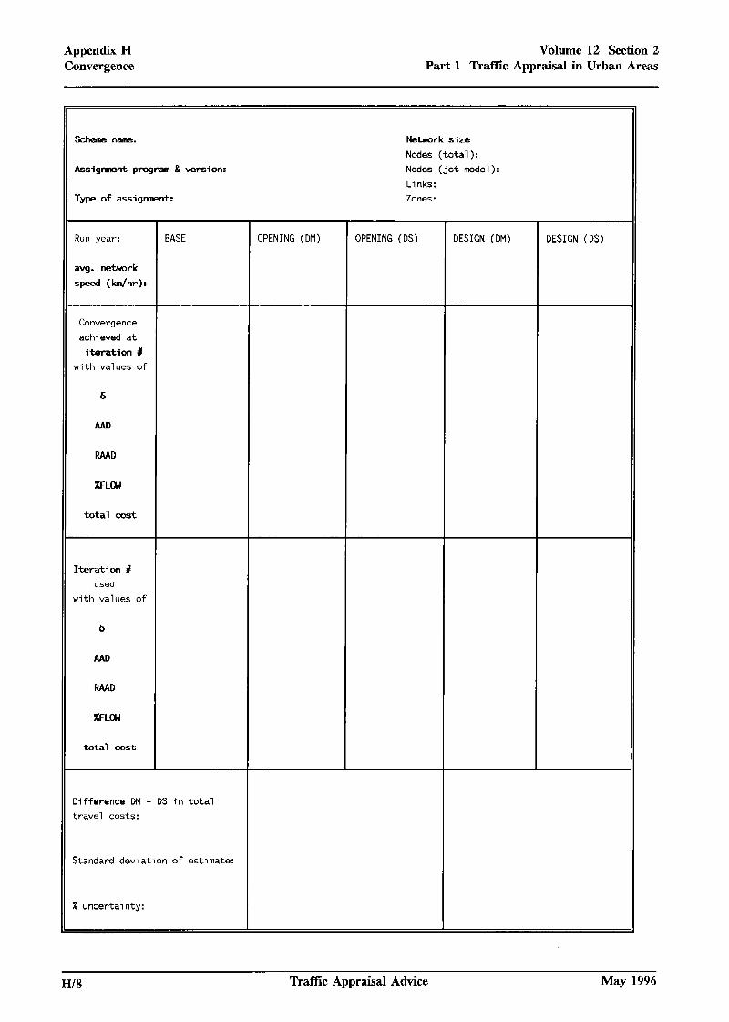
Appendix H Volume 12 Section 2 Convergence Part 1 Traffic Appraisal in Urban Areas
?dlena nanva:
Assigmnt prqram & version:
Type of assignment:
Mehark size
Nodes (total ) :
Ndes (jet model):
Links:
Zones :
Run year: BASE OPENING (DM) OPENING (DS) DESIGN (DM) DESIGN (DS)
avg. netrmrk
sped (km/hr):
Convergence
achieved at
iteration #
with values of
6
MD
WAD
XFLCM
total cost
Iteration R
used
with values of
6
MD
RAAD
ZFLCM
teal cost
Difference DM - DS in total
travel costs:
Standard deviation of estimate:
X uncertainty:
H/8 Traffic Appraisal Advice May 1996