1

DNA Genealogy, Mutation Rates, and Some Historical Evidences Written in Y-Chromosome. I. Basic Principles and the Method Anatole A. Klyosov1

Abstract

Origin of peoples in a context of DNA genealogy is an assignment of them to a

particular tribe (all members of which belong to a certain haplogroup) or its

branch (a lineage), initiated in a genealogical sense by a common ancestor, and an

estimation of a time span between the common ancestor and its current

descendants. At least two stumbling blocks in this regard are as follows: (1)

sorting out haplotypes from a random series in order to assign them to their

proper common ancestors, and (2) an estimation of a “calibrated” time span from

a common ancestor. The respective obstacles are (1) random series of haplotypes

are often descend from a number of common ancestors, which – as a result of

non-critical approaches in calculations – superimpose to a some “phantom

______________________________________________________________

1 Anatole Klyosov, 36 Walsh Road, Newton, Massachusetts 02459, USA

aklyosov@comcast.net; Phone (617)785-4548; Fax (617)964-4983

2

common ancestor”, and (2) mutation rates depend on a set of markers employed,

and on a “definition” of a generation length, let alone some “evolutionary” and

“pedigree-based” mutation rates lacking a clear explanation when either of them

can and should be employed. We have developed a convenient approach to

kinetics of haplotype mutations and calculating the time span to the common

ancestor (TSCA) using both established and modified theoretical methods (Part I)

and illustrated it with a number of haplotype series related to various populations

(Part II). The approach involves both the “logarithmic” (no mutation count) and

the “linear” “mutation-count” procedures as complementary to each other, along

with a separation of genealogical lineages as branches on a haplotype tree, each

having its base (ancestral) haplotype. Besides, we have advanced the “linear”

approach employing a correction of dating using the degree of asymmetry of

mutations in the given haplotype series, and a correction for reverse mutations,

using either a mathematical formula or a reference Table. It was compared with

the ASD (average square distance) method, using both base haplotypes and a

permutational ASD method (no ancestral haplotypes employed), and showed that

the “linear” method has a lower error margin compared to the ASD, while the

ASD method does not require corrections for back mutations, however, its

outcome does depend on a symmetry of mutations (not the permutational

method). Therefore, both “linear” and the ASD methods are complementary to

each other.

3

A convenient formula was suggested for calculations of standard deviations for

an average number of mutations per marker in a given series of haplotypes and

for a time span to the common ancestor, and it was verified using the Bayesian

posterior distribution for the time to the TSCA, taking into account the degree of

asymmetry of the given haplotype series. A list of average mutations rates for 5-,

6-, 7-, 9-, 10-, 11-, 12-, 17, 19-, 20-, 25-, 37- and 67-marker haplotypes was

offered for calculations of the TSCA for series of haplotypes.

Introduction

Origin of peoples in a context of DNA genealogy involves an assignment of each

of them to a particular tribe or its branch (lineage) descending from a particular

ancestor who had a base (“ancestral”) Y-STR haplotype. Of particular interest is

an estimation of a time span between the common ancestor and its current

descendants. If information obtained this way can be presented in a historical

context and supported, even arguably, by other independent archeological,

linguistic, historical, ethnographic, anthropological and other related

considerations, this can be called a success.

Principles of DNA genealogy have been developed over the last decade

and volumes can be written on each of them. The main principles are

4

summarized briefly below (Nei, 1995; Karafet et al., 1999; Underhill et al., 2000;

Semino et al., 2000; Weale, et al., 2001; Goldstein et al., 1995a; Goldstein et al.,

1995b; Zhivotovsky & Feldman, 1995; Jobling & Tyler-Smith, 1995; Takezaki

& Nei, 1996; Heyer et al., 1997; Skorecki et al., 1997; Thomas et al., 1998;

Thomas et al., 2000; Nebel et al., 2000; Kayser et al., 2000; Hammer et al., 2000;

Nebel et al., 2001).

First- Fragments of DNA (haplotypes) considered in this study have

nothing to do with genes. Technically, some of them can be associated with gene

fragments. However, those arguable associations are irrelevant in context of this

study.

Second- Copying of the Y chromosome from father to son results in

mutations of two kinds, single nucleotide polymorphisms (SNP) which are certain

inserts and deletions in Y chromosomes and mutations in short tandem repeats

(STR), which make them shorter or longer by certain blocks of nucleotides. A

DNA Y-chromosome segment (DYS) containing an STR is called a locus, or a

marker. A combination of certain markers is called a haplotype.

Third- All people (males in this context) have a single common ancestor

who lived by various estimates between 50,000 and 90,000 years ago. This time

is required to explain variations of haplotypes in all tested males.

Fourth- Haplotypes can be practically of any length. Typically, the

shortest haplotype considered in DNA genealogy is a 6-marker haplotype (though

5

an example of a rather obsolete 5-marker haplotype is given in Table 1 below). It

used to be the most common in peer-review publications on DNA genealogy

several years ago, then it was gradually replaced with 9-, 10-, and 11-marker

haplotypes, and lately with 17-, 19- and 20-marker haplotypes, see Table 1.

Twelve-marker haplotypes are also often considered in DNA genealogy;

however, they are rather seldom presented in academic publications. For

example, a common 12-marker haplotype is the “Atlantic Modal Haplotype” (in

haplogroup R1b1b2 and its subclades):

13-24-14-11-11-14-12-12-12-13-13-2

In this case, the order of markers is different when compared with the 6-marker

haplotypes (typically DYS 19, 388, 390, 391, 392, 393), and it corresponds to the

so-called FTDNA standard order: DYS 393, 390, 19, 391, 385a, 385b, 426, 388,

439, 389-1, 392, 389-2.

In a similar manner, 17-, 19-, 25-, 37-, 43- and 67-marker haplotypes have

been used in genetic genealogy, which is of the same meaning as that in the DNA

genealogy. On average, when large haplotype series are employed, containing

thousands and tens of thousands of alleles one mutation occurs once in: 2,840

years in 6-marker haplotypes, shown above, 1,140 years in 12-marker haplotypes,

740 years in 17-marker haplotypes (Y-filer), 880 years in 19-marker haplotypes,

6

540 years in 25-marker haplotypes, 280 years in 37-marker haplotypes, and 170

years in 67-marker haplotypes, using the mutation rates given in Table 1. This

gives a general idea of a time scale in DNA genealogy. Specific examples are

given below for large and small series of haplotypes.

Fifth- However, the above times generally apply on average only to a

group of haplotypes, whereas a pair of individuals may have large differences

with these values since the averaging process is more crude. One cannot calculate

an accurate time to a common ancestor based upon just a pair of haplotypes,

particularly short haplotypes. As it is shown below in this paper, one mutation

between two of 12-marker haplotypes (of the same haplogroup or a subclade)

places their most recent common ancestor between 1,140 ybp and the present

time (the 68% confidence interval) or between 1725 ybp and the present time (the

95% confidence interval). Even with four mutations between two of 12-marker

haplotypes their common ancestor can be placed – with 95% confidence –

between 4575 ybp and the present time, even when the mutation rate is

determined with the 5% accuracy. On the other hand, as it will be shown below,

with as many as 1527 of 25-marker haplotypes, collectively having almost 40

thousand alleles, the standard deviation (SD) of the average number of mutations

per marker is as low as ±1.1% at 3500 years to the common ancestor, and the

uncertainty of the last figure is determined by only uncertainly in the mutation

rate employed for the calculation. Similarly, with 750 of 19-marker haplotypes,

7

collectively having 14,250 alleles, the SD for the average number of mutations

per marker equals to ±2.0% at 3600 years to the common ancestor.

As one can see, mutations are ruled by statistics and can best be analyzed

statistically, using a large number of haplotypes and particularly when a large

number of mutations in them. The smaller the number of haplotypes in a set and

the smaller the number of mutations, the less reliable the result. A rule of thumb,

supported by mathematical statistics (see below) tells us that for 250 alleles (such

as in ten 25-marker haplotypes, 40 of 6-marker haplotypes, or four 67-marker

haplotypes), randomly selected, a standard deviation of an average number of

mutations per marker in the haplotype series is around 15% (actually, between 11

and 22%), when its common ancestor lived 1,000 – 4,000 years before present.

The less amount of the markers, the higher the margin of error.

Sixth- An average number of STR mutations per haplotype can serve to

calculate the time span lapse from the common ancestor for all haplotypes in the

set, assuming they all derived from the same common ancestor and all belong to

the same clade. That ancestor had a so-called base, or ancestor (founder)

haplotype. However, very often haplotypes in a given set are derived not from

one common ancestor from the same clade, but represent a mix from ancestors

from different clades.

Since this concept is very important for the following theoretical and

practical considerations in this work, it should be emphasized that by a “common

8

ancestor for a series of haplotypes” we understand haplotypes directly discernable

from the most recent common ancestor. Such series of haplotypes are called

sometimes “a cluster”, or “a branch”, or “a lineage”. Each of them should have a

founding haplotype motif, and the founding haplotype is called the base

haplotype. Each “cluster”, or “branch”, or a “uniform” series of haplotypes

typically belong to the same haplogroup, marked by the respective SNP (Single

Nucleotide Polymorphism) tag, and/or to its downstream SNP’s, or clades.

Granted, any given set of haplotypes has its common ancestor, down to

the “Chromosomal Adam”. However, when one tries to calculate a time span to a

[most recent] “common ancestor” for an assorted series of haplotypes, which

belong to different clades within one designated haplogroup, or to different

haplogroups, he comes up with a “phantom common ancestor”. This “phantom

common ancestor” can have practically any time span separating it from the

present time, and that “phantom time span” would depend on a particular

composition of the given haplotype set.

Since descendants retain the base haplotype, which is relayed along the

lineage from father to son, and mutations in haplotypes occur on average once in

centuries or even millennia, then even after 5000 years, descendants retain 23%

of the base, ancestral, unchanged 6-marker haplotype. In 12-marker haplotypes,

theoretically 23% of the descendants of the founder will still have the base

9

haplotype after 1,800 years. As it is shown below in this paper, this figure is

supported by actual, experimental data.

Seventh- The chronological unit employed in DNA genealogy is

commonly a generation. The definition of a generation in this study is an event

that occurs four times per century. A “common” generation cannot be defined

precisely in years and floats in its duration in real life and it depends on time in

the past, on culture of the given population, and on many other factors. Generally,

a “common” generation in typical male lineages occurs about three times per

century in recent times, but may be up to four times (or more) per century in the

pre-historic era. Furthermore, generation times in specific lineages may vary.

Hence, it does not have much sense for calculation in DNA genealogy to rely on

so vaguely “defined” factor as “duration of a common generation”.

In this study “generation” is the calculus term, it is equal exactly to 25

years, and represents the time span used for the calibration of mutation rates.

Again, many argue that a generation often is longer than 25 years, and point at

33-35 years. However, it is irrelevant in the presented context. What is actually

matters in the calculations is the product (n·k), that is a number of generations by

the mutation rate. If the mutation rate is, say, 0.0020 mutations per 25 years (a

generation), it is 0.0028 per 35 years (a generation), or 0.0080 per 100 years (a

“generation”). The final results in years will be the same. A different amount of

years per generation would just require a recalculation of the mutation rate

10

constant for calibrated data. A “years in a generation” is a non-issue, if calibrated

data are employed.

Eighth- Particular haplotypes are often common in certain territories. In

ancient times, people commonly migrated by tribes. A tribe was a group of

people typically related to each other. Their males shared the same or similar

haplotypes. Sometimes a tribe population was reduced to a few, or even to just

one individual, passing though a so-called population bottleneck. If the tribe

survived, the remaining individual or group of individuals having certain

mutations in their haplotypes passed their mutations to the offspring. Many

members left the tribe voluntarily or by force as prisoners, escapees, through

journeys, or military expeditions. Survivors continued and perhaps initiated a

new tribe in a new territory. As a result, a world DNA genealogy map is rather

spotty, with each spot demonstrating its own prevailing haplotype, sometimes a

mutated haplotype, which deviated from the initial, base, ancestral haplotype. The

most frequently occurring haplotype in a territory is called a modal haplotype. It

often, but not necessarily, represents the founder’s ancestral haplotype.

Ninth- People can be assigned to their original tribes of their ancestors

not only based on their haplotypes, but based on their SNP’s, which in turn lead

to their haplogroups and sub-haplogroups, so-called clades. SNP mutations are

practically permanent. Once they appear, they remain. Theoretically, some other

mutations can happen at the same spot, in the same nucleotide, changing the first

11

one. However, with millions of nucleotides such an event is very unlikely. There

are more than three million chromosomal SNP’s in the human genome (The

International HapMap Consortium, 2007), and DNA genealogists have employed

a few hundreds of them.

Examples include haplogroups A and B (African, the oldest ones),

haplogroups C (Asian, as well as a significant part of Native Americans,

descendants of Asians), haplogroups J (Middle Eastern) with J1 (mainly Semitic,

including both Jews and Arabs), and J2 (predominantly Mediterranean, including

also many Turks, Armenians, Jews). Others include haplogroups N (represented

in many Siberian peoples and Chinese, as well as in many Northern Europeans)

and haplogroup R1b and its subgroups are observed primarily, but not

exclusively, in Western Europe, Asia, and Africa. Haplogroup R1a1 dominates

in Eastern Europe and Western Asia, with a minute percentage along the Atlantic

coast. R1a1 represents close to 50% (and higher) of the population in Russia,

Ukraine, Poland, and the rest of Eastern Europe, and 16% of the population in

India. Haplogroup R1a1 also occurs in some areas in Central Asia particularly in

Kirgizstan and Tadzhikistan.

In other words, each male has a SNP from a certain set, which assigns his

patrilineal lineage to a certain ancient tribe.

Tenth- It is unnecessary to have hundreds or thousands of different

haplotypes in order to determine an ancestral (base) haplotype for a large

12

population and calculate a time span from its common ancestor to the present

time. Alleles in haplotypes do not have random values. Rather, they are typically

restricted in rather narrow ranges. Then, after thousands of years descendants of

common ancestors for whole populations of the same haplogroup have typically

migrated far and wide. In Europe, for example, one can hardly find an enclave in

which people have stayed put in isolation for thousands of years. Last but not

least, wherever bearers of haplotypes are hiding, their mutations are “ticking”

with the same frequency as the mutations of anyone else.

For example, an ancestral (base) haplotype of the Basques of haplogroup

R1b1b2, deduced from only 17 of their 25-marker haplotypes (see below) follows

(in the FTDNA order):

13-24-14-11-11-14-12-12-12-13-13-29-17-9-10-11-11-25-14-18-29-15-15-17-17

This base haplotype is very close to a deduced haplotype (Klyosov, 2008a) of a

common ancestor of 184 individuals, who belong to haplogroup R1b1b2,

subclade U152:

13-24-14-11-11-14-12-12-12-13-13-29-17-9-10-11-11-25-15-19-29-15-15-17-17

13

Two different alleles (in bold) differ between the two base haplotypes and have

average values of 14.53 and 18.35 in the Basques, while in subclade U152 the

average values are 14.86 and 18.91, respectively. Adding the two differences we

get 0.89 mutations total between the 25-marker haplotypes. This amount of

difference between two founding haplotypes would suggest only approximately

ten generations between them, using a method to be presented shortly. However,

a margin of error will be significantly higher when, e.g., 425 alleles are

considered (17 of 25-marker haplotypes) compared to 14,250 alleles (750 of 19-

marker haplotypes), as in the following example.

All (or most of them) of as many as 750 of 19-marker Iberian R1b1

haplotypes, published in (Adams et al, 2008), descended from the following base

(ancestral) haplotype, shown here in the same format as the above:

13-24-14-11-11-14-X-12-12-13-13-29

The base haplotype on the first 12 markers is exactly the same, plus the

only marker, DYS437, from the second FTDNA panel, determined in the 19-

marker haplotype series, is also “15” in the base Iberian haplotype in both 25- and

19-marker formats. As it will be shown below, an average number of mutations

in these two series of Basque haplotypes, seventeen 25- and seven hundred fifty

19-markers ones, is also practically the same: 100 mutations in the first series and

14

2796 mutations in the second series give, respectively, 0.257 and 0.262 after

normalizing for their average mutation rates (see Table 1). However, the margin

of error is much lower in the second case. It will be considered in detail below.

This kind of a comparison would, however, be misleading when

comparing haplotypes of two individuals on or near the modal values of a

haplogroup (Nordtvedt, 2008). As it was stated above (section Fifth), mutations

are ruled by statistics and can best be analyzed statistically, using a number of

haplotypes, not just two, as it was demonstrated above using 17 Basque,, 184

subclade U152, and 750 Basque haplotypes from three different series.

To further illustrate the example, consider 12,090 of 25-marker R1b

haplotypes (including subclades) from the YSearch database. When combined,

they have the following modal (base) haplotype:

13-24-14-11-11-14-12-12-12-13-13-29-17-9-10-11-11-25-15-19-29-15-15-17-17

This is exactly the same base haplotype as shown above for R1b1b2-U152, and

practically the same for that for the Basques of haplogroup R1b1b2. Furthermore,

as it is shown below, common ancestors of the 17 Basques, 750 Basques, 184

bearers of U152 subclade, and 12,090 bearers of R1b haplogroup lived in about

the same time period, within less than a thousand years.

15

The power of DNA genealogy is not in large numbers, though they are

always welcomed and greatly reduce the standard deviation of the TSCA, but in

randomness of haplotype selections. Again, that power can be significantly

reduced when small haplotype series (with less than 250 alleles collectively, see

above) are employed.

Eleventh- Unlike languages, religion, cultural traditions, anthropological

features, which are often assimilated over centuries and millennia by other

languages, cultures, or peoples, haplotypes and haplogroups cannot be

assimilated. They can be physically exterminated, though, and haplotype trees

very often point at extinct lineages. This non-assimilation makes haplogroups and

haplotypes practically priceless for archaeologists, linguists, and historians. They

not only stubbornly transcend other assimilations across millennia, but also

provide means for calculations of when, and sometimes where, their common

ancestors lived.

Methods

We will discuss several methods for calculating time spans to common ancestors

(TSCA) for a given series of haplotypes. Underlying principles of the methods

are well established, and all are based on a degree of microsatellite variability and

“genetic distances” by counting a number of mutations in various loci and

conducting their statistical evaluation. In principle, either of the methods may be

16

used, and they should – theoretically – yield approximately the same result. In

reality, they do not, and results vary greatly, often by hundreds per cent, when

presented by different researchers, even when practically the same populations

were under study.

The main reasons of such a discrepancy are typically as follows: (a)

different mutation rates employed by researchers, (b) lack of calibration of

mutation rates using known genealogies or known historical events, or when a

time depth for known genealogies was insufficient to get all principal loci

involved, (c) mixed series of haplotypes, which are often derived from different

clades, and in different proportions between those series, which directly affect a

number of mutations in the series, (d) lack of corrections for reverse mutations

(ASD-based calculations [see below] do not need such a correction), (e) lack of

corrections for asymmetry of mutations in the given series of haplotypes – in

some cases.

All these issues are addressed in this study. Besides, a different in kind

method was applied to calculating “age” of a common ancestor. This method is

based not on mutations counting, but on base haplotypes counting in a series of

haplotypes. This method does not suffer from “asymmetry” of mutations, or from

multiple mutations of the same marker, and does not consider which mutations to

include and which to neglect in a total count of mutations. It’s the only principal

limitation is that it requires an appreciable number of base haplotypes in the

17

series, preferably more than four or five. Naturally, the longer the haplotypes in

the series, the less of the base haplotypes the series retains. However, for

extended series of haplotypes said restriction can be alleviated. For example, said

19-marker haplotypes in the 750-haplotype Iberian R1b1 series contains 16

identical, base haplotypes, shown above. A series of 857 English 12-marker

haplotypes contains 79 base haplotypes (Adamov and Klyosov, 2009b). While a

series of 325 of Scandinavian I1 25-marker haplotypes contained only two base

haplotypes, the same series of 12-marker haplotypes contained as many as 26

base haplotypes. In fact, all four cases (12- and 25-marker haplotypes, in which

calculations employed “mutation counting” and “base haplotypes counting”) gave

pretty much similar results, equivalent to 0.210, 0.238, 0.222, and 0.230

mutations per marker, on average 0.225±0.012, that is with 5.3% deviation. This

deviation (the standard error of the mean) corresponds to 5.3 %6.104

standard deviation for the average number of mutations per marker, which is

similar to those calculated and reported below in this paper. This standard

deviation includes those for the both two different procedures (counting

mutations and counting non-mutation haplotypes), and mutation rates for 12- and

25-marker haplotypes.

Probabilities of mutations, or mutation rates in haplotypes can be

considered from quite different angles, or starting from different paradigms. One

of them assumes that a discrete probability distribution of mutations in a locus (or

18

an average number of mutations in a multi-loci haplotype), that is a probability of

a number of independent mutations occurring with a known average rate and in a

given period of time, is described by the Poisson distribution

ktm

em

ktmP !)()(

where:

P(m) = a probability of appearance of “m” mutations in a marker (or haplotype),

m = a number of mutations in a marker (or haplotype),

k = average mutation rate per generation,

t = time in generations.

As an example, for k = 0.022 mutations per 12-marker haplotype per

generation (Table 1), a 100-haplotype series will contain 80 base (unchanged,

identical) haplotypes (m=0) after 10 generations, since e-0.22 = 0.8.

Another approach employs a binomial theorem, according to which a

fraction of haplotypes with a certain number of mutations in a series equals

mmt

qmmt

ptmP!)!(

!)()(

where:

19

m = a number of mutations,

q = probability of a mutation in each generation,

t = time in generations,

p = 1-q

Similarly with the above example, for q = 0.022 mutations per 12-marker

haplotype per generation (Table 1), a 100-haplotype series will contain 80 base

(unchanged) haplotypes (m=0) after 10 generations, since 0.97810 = 0.8.

The third approach, which I employ in this work due to its simplicity and

directness, is the “logarithmic” approach. It states that a transition of the base

haplotypes into mutated ones is described by the first-order kinetics:

B = Aekt, (1)

that is

ln(B/A) = kt (2)

where:

B = a total number of haplotypes in a set,

A = a number of unchanged (identical, not mutated) base haplotypes in the set

20

k = an average mutation rate (frequency), which is, for example, 0.0088, 0.022,

0.034, 0.0285, 0.046, 0.090, and 0.145 mutations per haplotype per generation

for a 6-, 12-, 17-, 19-, 25-, 37- and 67-marker haplotype, respectively (Table 1).

t = a number of generations to the common ancestor for the whole set of

haplotypes (without corrections for back mutations).

For the example given above it shows that for a series of 100 of 12-

marker haplotypes (the average mutation rate of 0.022 mutations per haplotype

per generation),

ln(100/80)/0.022 = 10 generations.

It is exactly the same number at those obtained by the Poisson distribution and

the binomial theorem described above.

Needless to say, that all the above three approaches stay on the same

mathematical basis, and, as it was said above, are presented at three different

angles at the calculations.

Following the introduction of this and other methods (the “linear” method

along with a correction for back mutations, and two ASD [average square

distance] methods, along with dissection of haplotype trees into branches, or

lineages, and their separate analysis), Table 2 below is provided that will make it

21

possible to avoid most of the math that is involved to make corrections for

reverse mutations.

Principles of the “logarithmic” method for calculating a timespan to the

common ancestor. Either of two methods – the logarithmic and the linear

(mutation-counting) – for calculating a time span to the common ancestor may be

used, but with one condition: they both should give approximately the same

result. This is important, since both of them are based on quite different

methodology. If the two methods yield significantly different results, for

example, different by a factor of 1.5, 2 or more, then the haplotype series

probably represents a mixed population, that is haplotypes of different clades,

clusters, lineages. Or it might signal of some other details of the genealogy or

population dynamics, which is inconsistent with one lineages, and will result in a

“phantom common ancestor”. In this case it will be necessary to divide the group

appropriately into two or more subgroups and to treat them separately. A

haplotype tree is proven to be very effective in identifying separate lineages, as

will be shown in the subsequent paper (Part II).

This is a brief example to illustrate this important principle. Let us

consider two sets of 10 haplotypes in each:

14-16-24-10-11-12 14-16-24-10-11-12

14-16-24-10-11-12 14-16-24-10-11-12

22

14-16-24-10-11-12 14-16-24-10-11-12

14-16-24-10-11-12 14-16-24-10-11-12

14-16-24-10-11-12 14-16-24-10-11-12

14-16-24-10-11-12 14-16-24-10-11-12

14-17-24-10-11-12 14-16-25-9-11-13

15-16-24-10-11-12 14-16-25-10-12-13

14-15-24-10-11-12 14-17-23-10-10-13

15-17-24-10-11-12 16-16-24-10-11-12

The first six haplotypes in each set are base (ancestral) haplotypes. They are

identical to each other. The other four are mutated base haplotypes or admixtures

from descendant haplotypes of a different common ancestor. A number of

mutations in the two sets with respect to the base haplotypes are 5 and 12,

respectively. If to operate only with mutations, the apparent number of

generations to a common ancestor in the sets is equal to 5/10/0.0088 = 57

generations and 12/10/0.0088 = 136 generations, respectively (without a

correction for back mutations). However, in both cases a ratio of base haplotypes

gives us a number of generations equal to ln(10/6)/0.0088 = 58 generations

(principles of calculations are described above). Hence, only the first set of

haplotypes gave close to a matching numbers of generations (57 and 58) and

represents a “clean” set, having formally one common ancestor. The second set is

23

“distorted”, or “mixed”, as it certainly includes descendant haplotypes from

apparently more than one common ancestor. Hence, it cannot be used for

calculations of a number of generations to a common ancestor.

An advantage of the “logarithmic” method is that there is no risk of

counting the same mutation multiple times; one counts only an amount of

unchanged (base) haplotypes in the series. For example, Fig. 2 below shows a

haplotype tree of the Donald Clan 25-marker haplotypes. There are 84 haplotypes

in the series, and 21 of them are identical to each other. Hence, ln(84/21)/0.046 =

30 generations to a common ancestor. All those 84 haplotypes contain 109

mutations, this gives 109/84/0.046 = 28 generations to a common ancestor. 0.046

mutations per 25-marker haplotype per generation is the average mutation rate

constant (Table 1). Hence, the above calculations give three pieces of evidence:

(1) reliability of the calculations, (2) a proof of a single common ancestor in the

series of 84 haplotypes, (3) approximately 29±2 generations to a common

ancestor, if not to consider the standard deviation for the figure, based on the

margin of error of the average number of mutations per marker, and of the

employed mutation rate. This example will be considered in more detail below.

However, it should be noticed here that the 28 generations obtained by the linear

method should carry the standard deviation, which in this particular case is 28±4

generations. It is based on 9.6% standard deviation for the average number of

24

mutations per marker, and 13.9% standard deviation for the mutation rate, all for

the 95% confidence interval. The theory behind it is considered below.

Lately four more mutated haplotypes were added to the Donald Clan

series. 21 base haplotypes stay the same, and all 88 haplotypes contain 123

mutations. This gives ln(88/21)/0.046 = 31 generations, and 123/88/0.046 = 30

generations to a common ancestor. It still holds the preceding value of 29±2

generations to a common ancestor without considering the “experimental”

standard deviation, and 30±4 generations with that consideration.In the last case,

with the inclusion of four additional haplotypes, the two standard deviations

described above became 9.0% and 13.5%, respectively. It will be explained

below.

Table 1 shows average mutation rates per haplotype and per marker for

haplotypes of various lengths. Table 2 shows corrections for reverse mutations.

Mutation rates for 5-, 6-, 7-, 9-, 10-, 11-, and 12-marker haplotypes are calculated

in accordance with Chandler’s data (Chandler, 2006). Mutation rates for 17-, 19-,

20-, 25-, 37- and 67-marker haplotypes are obtained via calibration, primarily

using the Donald Clan haplotypes and verified, when possible, with Chandler’s

data, as illustrated above and described in detail earlier (Klyosov, 2008a, 2008b,

2008c; Adamov & Klyosov, 2008a). Findings conclude that average mutation

rates per marker for 12- and 25-marker haplotypes are equal to each other

(0.00183 mutations per marker per generation), and that for 17-marker haplotypes

25

equals to 0.00200 mutations per marker per generation. Mutation rates for 37-

and 67-marker haplotypes equal 0.00243 and 0.00216 mutations per marker per

generation, respectively (Klyosov, 2008a, 2008b, 2008c; Adamov & Klyosov,

2008a).

The calibration made unnecessary to consider separately “slow” or “fast”

markers and discuss how they can impact calculations. The calibration showed

that 37- and 67-marker haplotypes have the average mutation rate of 0.09 and

0.145 mutations per haplotype per generation of 25 years. Practical examples

given in the subsequent paper (Part II) show that all these average mutation rates

agree well with each other. In many cases calculations of a series of haplotypes

for the same population, using 12-, 17-, 19-, 25-, 37- and 67-marker haplotypes,

results practically in the same time span to a common ancestor. Sometimes (but

not always) 12-marker haplotypes give lower time spans compared with 25- and

37-marker haplotypes. 25-, 37- and 67-marker haplotypes commonly agree well

with each other.

Calibration of 17-marker haplotypes (Y-filer) using the Donald Clan

haplotype series, and comparison of them with 25- and 37-marker haplotype

series have a surprisingly convenient, “classical” average mutation rate of 0.002

mutations per marker per generation, that is 0.034 mutations per haplotype per

generation.

26

According to John Chandler (2006), his average mutation rate values for

25- and 37-marker haplotypes were 0.00278±0.00042 and 0.00492±0.00074 per

marker per generation, that is 0.070 and 0.180 mutations per haplotype per

generation. They are much too high compared with the respective calibrated rates

of 0.00183 and 0.00243 mut/marker/gen and 0.046 and 0.090 mut/haplotype/gen,

employed in this and the subsequent paper. They would not result in the same

time spans to a common ancestor for 25- and 37-marker haplotypes. Apparently,

the “summation” of individual mutation rates for individual markers works only

for the first 12 markers (in the FTDNA order). There the calibrated value of

0.00183 mut/marker/gen, employed in this work, is within the error margin with

the Chandler’s 0.00187±0.00028 value. Summation of the 25 markers by

Chandler gives 0.00278±0.00042, which the calibrated value employed in this

work results in the much lower value of 0.00183 mut/marker/gen, more than 50%

difference. Outcomes of such a difference, based on actual haplotype series, are

given below.

Apparently, not all individual mutation rates can be and should be

summed up. It gives an “upper hand” to fast markers. For example, in the

Chandler’s table just four DYS464 markers (total mutation rate of 0.00566x4 =

0.02264) exceed by rate the whole first (1-12 markers) panel (0.02243). With

such a “background” for 25-marker haplotypes mutations in the first panel

become insignificant in the whole balance of mutations. Examples of comparative

27

applications of the Chandler’s average mutation rates to actual series of

haplotypes are given below.

Procedure for a calculation of a timespan to a common ancestor of a

series of haplotypes. Logistics of DNA genealogy requires a set, or a sequence,

of rather simple steps which would simplify a calculation of a timespan to a

common ancestor for a given series of haplotypes. Here are suggested steps to

follow:

First: Make sure that the series of haplotypes under consideration is

derived each from a single common ancestor, not from a variety of “common

ancestors”. “Variety” for the purposes of this discussion is defined as a

minimum of two. Clearly, a “common ancestor” is a euphemism and can

include brothers or/and close male relatives, which cannot be resolved by

contemporary methods of DNA genealogy. By a “common ancestor” we assume

an individual and his close relatives which are the bearers of an ancestral

haplotype, which in turn served as a base for consequent branching via mutations

in loci of the ancestral haplotype. Those branchings have led to a series of

haplotypes under consideration. In order to make sure that the series is derived

from a single “common ancestor”, we can employ a few criteria.

The first criterion is to analyze a haplotype tree. In case of one common

ancestor, the tree will ascend to one “root” at the trunk of the tree. If two or more

separate roots are present, each with separate branches, the construction would

28

point to separate “common ancestors”. All of them, if within one haplogroup,

have their “common ancestor”. This may occur within several haplogroups as

well. However, a given haplotype series should be treated separately, with one

common ancestor at a time. Otherwise some “phantom common ancestor” will be

numerically created, typically as a superposition of several of them.

A “base” haplotype can be equivalent to the ancestral one, or it can be its

approximation, particularly when it does not present in multiple copies in the

considering series of haplotypes. Hence, two different terms, “ancestral

haplotype” and “base haplotype” can be utilized.

The simplest and the most reliable way to identify an ancestral (base)

haplotype is to find the most frequently repeated copy in a given series of

haplotypes. It should be verified by using the so-called “linear” and “logarithmic”

models. According to the linear model:

n/N/µ = t

where n is a number of mutations in all N haplotypes in the given series of

haplotype, µ is an average mutation rate per haplotype per generation (Table 1),

and t is a number of generations to a common ancestor. Unlike the “linear”

model, the “logarithmic” one, as it was described above, considers a number of

29

base haplotypes in the given series, and does not count mutations. It employs the

following formula

ln(N/m)/µ = tln

where m is a number of base (identical) haplotypes in the given series of N

haplotypes, tln is a number of generations to a common ancestor. If t = tln (in a

reasonable range, for example, 10% of their values), then the series of haplotypes

is derived from the same common ancestors. If t and tln are significantly different

(for example, 150-200% or greater difference between them), the haplotype series

is certainly heterogeneous. Table 2 can be applicable only after separation of

haplotypes into several groups, each deriving from its common ancestor. For that

separation, the respective haplotype tree can be used (Klyosov, 2008a, 2008b,

2008c; Adamov & Klyosov, 2008a).

In other words, for a “homogeneous” series of haplotypes which are

derived from a single common ancestor, a number of mutations should be

compatible with a number of base haplotypes in the same series.

Second: Count a number of mutations in the “homogeneous” series

of haplotypes. This number should be counted with respect to the base

(ancestral) haplotype identified in the preceding step. All mutations should be

counted, considering them as independent ones. This is justified below.

30

Third: Calculate an average number of mutations per marker for all

haplotypes in the “homogeneous” series, as described in the preceding step. For

example, if there are 65 mutations per 20 of 7-marker haplotypes, then an average

number of mutation equals to 65/20/7 = 0.464±0.057 mutations per marker

accumulated during a timespan from a common ancestor. This figure is obtained

with the assumption of a full symmetry of the mutations (see below).

Fourth: Recalculate the average number of mutations, as described

in the preceding step, to the average mutations rate equal to 0.002 mutations

per marker per generation. The reason for this step is that each marker has its

own mutation rate. Different haplotypes contain different sets of markers and

therefore have different average mutation rates. These average mutation rates for

the mostly frequently used haplotypes are given in Table 1 below. For example,

for 7-marker haplotypes, considered in the above section (“Third”), the average

mutation rate per marker is not 0.00200, but 0.00186 mutation/marker/generation

(Table 1). It actually led to the accumulated 0.464 mutation/marker for a 7-

marker haplotype (see above). However, with the mutation rate of 0.002

mutations per marker per generation, there would be 0.464x0.002/0.00186 =

0.499±0.062 mutations/marker. One needs to do this recalculation in order to use

Table 2. Otherwise one needs to use 18 different tables for 18 types of haplotypes

in Table 1.

31

Fifth: Apply Table 2 to the obtained figure, in order to correct for

reverse mutations, which are accumulated in the haplotype for the time period

needed to generate all mutations in the given series of haplotypes. For example,

for an average number of accumulated mutations of 0.464±0.057 mutations per

marker in the 7-marker haplotype, recalculated to 0.499±0.062 mutations per

marker in an imaginary haplotype with 0.002 mutations per marker per

generation (see above), this corresponds to 331±53 generations or 8,275±1,320

years to a common ancestor. The timespan in years is calculated by assigning 25

years to a generation, as explained above.

If only the linear model is employed, without a consideration for reverse

mutations, then 65 mutations in 20 of 7-marker haplotypes would lead one to an

erroneous conclusion. The erred “result” would show only 65/20/0.013 = 250±40

generations (6,250±995 years) to a common ancestor, versus the more correct

331±53 generations (8,275±1,320 years) to a common ancestor. Formally, these

two figures are overlapping within their margins of error, however, the lower one

is still incorrect.

The same Table 2 considers contributions of reverse mutations into results

of the logarithmic model in which reverse mutations are not included. For

example, if the logarithmic model results in 250 generations to a common

ancestor, Table 2 shows that it corresponds to 331 generations, corrected for

reverse mutations.

32

In this study, haplotype trees were constructed using PHYLIP, the

Phylogeny Inference Package program (Felsenstein, 2005). A “comb” around the

wheel, a “trunk”, in haplotype trees identifies base haplotypes, identical to each

other and carrying no mutations compared to their ancestral haplotypes (see Fig.

2 below). The farther the haplotypes lies from the wheel, the more mutations they

carry compared to the base haplotype and the older the respective branch.

* * *

For more sophisticated researchers, three more steps in haplogroup

analysis are suggested below.

Sixth: Calculate a degree of asymmetry of the haplotype series under

consideration. A degree of asymmetry, when significant, affects a calculated

time span to a common ancestor at the same number of mutations in the

haplotype series. Generally, the more asymmetrical is the haplotype series (that

is, mutations are predominantly one-sided, either “up” or “down” from the base

haplotype), the more overestimated is the TSCA. Specific examples are

considered in the subsequent section.

The degree of asymmetry is calculated as a number of +1 or -1 mutations

(whichever is higher) from the base haplotype divided by a combined number of

+1 and -1 mutations. For a symmetrical haplotype series the degree of asymmetry

is equal to 0.5, as in the East European Slav R1a1 12- and 25-marker marker

haplotypes (see Part II). For a moderately asymmetrical series the degree of

33

asymmetry is equal to about 0.65, as in the R1b1b2 Basque 12-marker haplotype

series, though for the 17-marker extended haplotype series of 750 haplotypes it is

equal to 0.56 (see below). For a significantly asymmetrical series it is equal to

0.86, as in the N1c1 Yakut haplotype series (Adamov and Klyosov, 2008b), or to

0.87, as with the English I1 extended haplotype series (see below), and in

extreme cases approaches to 1.0

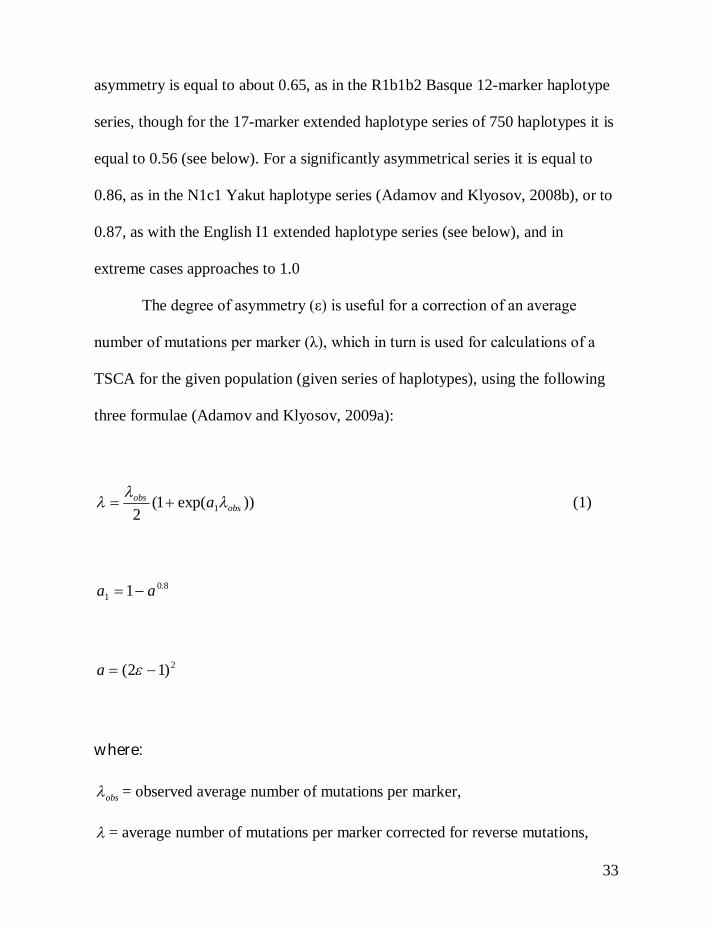
The degree of asymmetry (ε) is useful for a correction of an average

number of mutations per marker (λ), which in turn is used for calculations of a

TSCA for the given population (given series of haplotypes), using the following

three formulae (Adamov and Klyosov, 2009a):

))exp(1(2 1 obsobs a

(1)

8.01 1 aa

2)12( a

where:

obs = observed average number of mutations per marker,

= average number of mutations per marker corrected for reverse mutations,

34

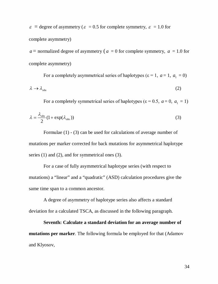
= degree of asymmetry ( = 0.5 for complete symmetry, = 1.0 for

complete asymmetry)

a = normalized degree of asymmetry ( a = 0 for complete symmetry, a = 1.0 for

complete asymmetry)

For a completely asymmetrical series of haplotypes (ε = 1, a = 1, 1a = 0)

obs (2)

For a completely symmetrical series of haplotypes (ε = 0.5, a = 0, 1a = 1)

))exp(1(2 obsobs

(3)

Formulae (1) - (3) can be used for calculations of average number of

mutations per marker corrected for back mutations for asymmetrical haplotype

series (1) and (2), and for symmetrical ones (3).

For a case of fully asymmetrical haplotype series (with respect to

mutations) a “linear” and a “quadratic” (ASD) calculation procedures give the

same time span to a common ancestor.

A degree of asymmetry of haplotype series also affects a standard

deviation for a calculated TSCA, as discussed in the following paragraph.

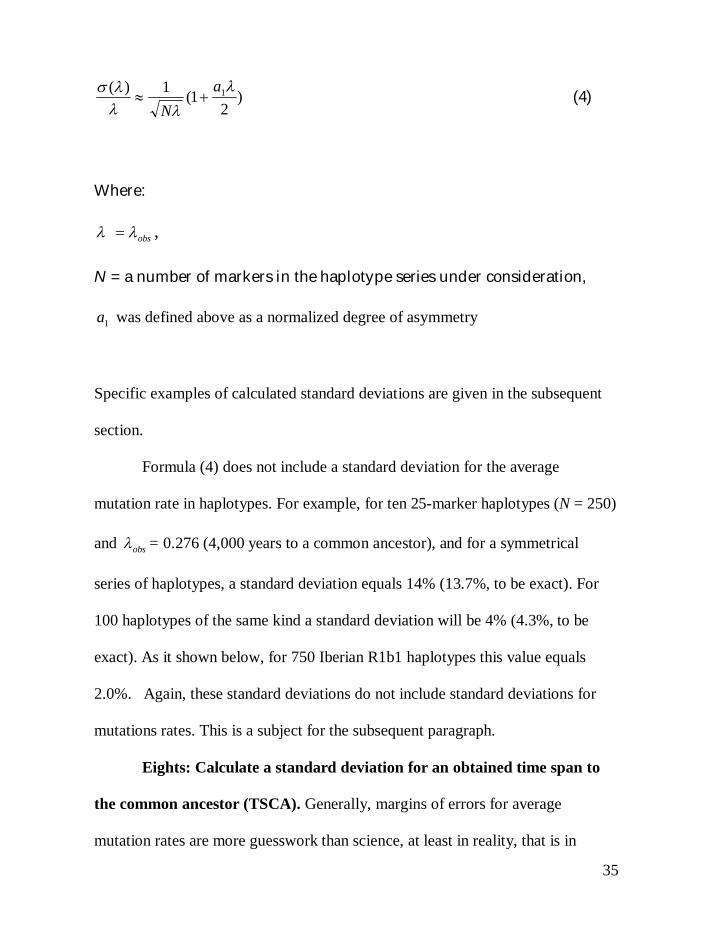
Seventh: Calculate a standard deviation for an average number of

mutations per marker. The following formula be employed for that (Adamov

and Klyosov,

35

)2

1(1)( 1

aN

(4)

Where:

obs ,

N = a number of markers in the haplotype series under consideration,

1a was defined above as a normalized degree of asymmetry

Specific examples of calculated standard deviations are given in the subsequent

section.

Formula (4) does not include a standard deviation for the average

mutation rate in haplotypes. For example, for ten 25-marker haplotypes (N = 250)

and obs = 0.276 (4,000 years to a common ancestor), and for a symmetrical

series of haplotypes, a standard deviation equals 14% (13.7%, to be exact). For

100 haplotypes of the same kind a standard deviation will be 4% (4.3%, to be

exact). As it shown below, for 750 Iberian R1b1 haplotypes this value equals

2.0%. Again, these standard deviations do not include standard deviations for

mutations rates. This is a subject for the subsequent paragraph.

Eights: Calculate a standard deviation for an obtained time span to

the common ancestor (TSCA). Generally, margins of errors for average

mutation rates are more guesswork than science, at least in reality, that is in

36

practical calculations, They probably vary between 5% and 15-20%. For the most

of mutation rates employed in this work I estimated the standard deviation as

10% for the 95% confidence interval (“two sigma”).

John Chandler in his study (Chandler, 2006) listed the mutation rates for

the FTDNA panels of 12, 25 and 37 markers as 0.00187±0.00028,

0.00278±0.00042, and 0.00492±0.00074, which gave a standard deviation as

exactly 15% in each case. Clearly, it is an assumed estimate rather than a

calculated value, since a mutation rate for 12 markers would be determined with a

different standard deviation compared to that for 25 or 37 markers, however, it

would be unrealistic to demand an exact value of standard deviation in those

cases. One would assume that a standard deviation for a whole panel of markers

would be lower than that for a each of the 37 markers determined separately and

then combined. Hence, a 5%-10% value for a standard deviation employed in this

study for a whole panel of haplotypes (as “one sigma” and “two sigma”), and for

that divided by a number of haplotypes in the panel can be considered as a

reasonable estimate. It is considered in more detail in the Discussion section

below.

At any rate, a standard deviation (SD) for the time span to the common

ancestor is based on the standard deviations for each of the two components, that

is the SD for the average number of mutations per marker (see above, Item 7) and

the SD for the average mutation rate for the given series of haplotypes. For

37

example, for R1b1 Iberian haplotypes (see above) a 68% confidence interval

(“one sigma”) for the TSCA would be equal to a square root of 0.012 + 0.12, that

is 10%, if we take the SD for the mutation rates in this case (19-marker

haplotypes) to be 10%. For the SD equaled to 5%, the 68% confidence interval

for the TSCA for the 750 Iberian haplotypes would be 5%. In other words, for

such numerous series of haplotypes, having one (in terms of DNA genealogy)

common ancestor, standard deviation for a time span to a common ancestor is

fully defined by the SD for the employed average mutation rate.

The 95% confidence interval (“two sigma”) for TSCA for the same R1b1

Iberian haplotypes would be equal to 10.2% (for the 10% standard deviation – as

“two sigma” – for the mutation rate). Again, even for such an extended and

symmetrical series of haplotypes, standard deviation for a time span to the

common ancestor is fully defined by the error margin for the employed average

mutation rate. Since I am inclined to a reasonable 5% SD in the mutation rate in

this work, the 95% confidence interval for the above case would be equal to a

square root of 0.022 + 0.12, that is ±10.2%, or 3,625±370 years before present

(see below).

Practical Examples

Let us consider four examples, the first one is so-called R1a1 Donald Clan

haplotype series, the second is the Basque R1b1b2 haplotype series in 12- and 25-

38

marker format, the third one is the Iberian R1b1 19-marker haplotypes, , and the

fourth one is the British Isles and Scandinavian I1 12- and 25-marker haplotype

series. The Iberian, the Isles and the Scandinavian haplotype series include

hundreds and well over a thousand of extended haplotypes.

R1a1 Donald haplotypes

There is a series of West European (by origin) haplotypes for which “classical”

genealogy data are known, so we can “calibrate” mutation rates we employ with

an actual timespan to a known common ancestor. The Donald extended family

haplotypes provide a good example (DNA-Project.Clan-Donald, 2008). Their

founding father, John Lord of the Isles, lived 26 generations ago (died in 1386)

(taking 25 years for generation, how it was explained above). Eighty four of 25-

marker haplotypes of his direct descendants are available (DNA-Project.Clan-

Donald, 2008), with all belonging to the R1a1 haplogroup.

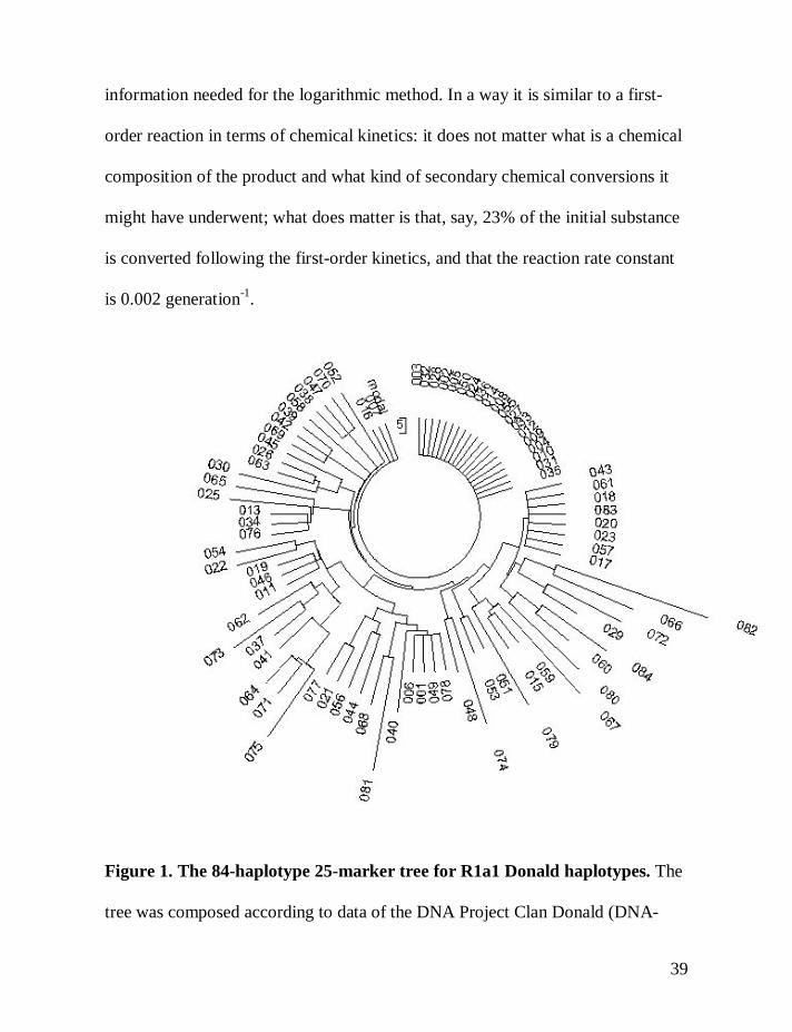
The haplotype tree is shown in Fig. 1. It illustrates a “classical” example

of a single common ancestor, since the tree in its entirety is base on one “stem”,

and includes a series of identical “base” haplotypes forming a “comb” on top of

the tree. As one can see, it does not matter for the logarithmic method which

“petals” (haplotypes) on the tree are longer and which are shorter, which in turn

reflects a number of mutations in them. The tree shows that 21 haplotypes are

ancestral ones, and the other 63 haplotypes are mutated. This is all the

39

information needed for the logarithmic method. In a way it is similar to a first-

order reaction in terms of chemical kinetics: it does not matter what is a chemical

composition of the product and what kind of secondary chemical conversions it

might have underwent; what does matter is that, say, 23% of the initial substance

is converted following the first-order kinetics, and that the reaction rate constant

is 0.002 generation-1.

Figure 1. The 84-haplotype 25-marker tree for R1a1 Donald haplotypes. The

tree was composed according to data of the DNA Project Clan Donald (DNA-

40

Project.Clan-Donald, 2008). The tree shows 21 identical “base” haplotypes sitting

on top of the tree.

The ancestral (base) haplotype for all 84 individuals is as follows:

13-25-15-11-11-14-12-12-10-14-11-31-16-8-10-11-11-23-14-20-31-12-15-15-16

The deviations (shown in bold) from the typical Isle base R1a1 haplotypes

(Klyosov, 2008e) are actually mutations the haplotype of the founding father

apparently had. All 84 haplotypes have 44 mutations in their 12-marker

haplotypes. This results in 0.0437±0.0066 mutations per marker on average, or

25±2 generations to the common ancestor with the 68% confidence interval, and

25±5 generations with the 95% confidence interval. In all 84 of 25-marker

haplotypes there were 109 mutations (with exclusion of several unusual 4-step

mutations), which gives 0.0519±0.050 mutations per marker, or 29±2 generations

to a common ancestor with the 68% confidence interval, and 29±4 generations

with the 95% confidence interval.. These results are close to the years of life of

the known common ancestor (26 generations ago).

A principally different approach to evaluation of a timespan to the

common ancestor is based not on counting mutations, but on counting of base,

non-mutated haplotypes in a haplotype set, as it was described above. This

41

approach is indifferent to “unusual” multistep mutations, since it considers only

“mutated” and “non-mutated” (base) haplotypes. Among all 84 Donald family

haplotypes there are 52 non-mutated 12-marker haplotypes, and 21 non-mutated

25-marker haplotypes. It gives ln(84/52)/0.022 = 22 generations, and

ln(84/21)/0.046 = 30 generations for 12- and 25-marker haplotypes, respectively.

This results in an average 26 ± 5 generations to a common ancestor, in a full

accord with “classical” genealogy.

Since the Chandler’s list of mutation rates provides with the average

mutation rates of 0.00187±0.00028 and 0.00278±0.00042 mutations per marker

in the 12- and 25-marker panel per generation (Chandler, 2006), it would result in

0.0437/0.00187 = 23±4 generations and 0.0519/0.00278 = 19±3 generations to

the common ancestor of the Donald Clan. with the 68% confidence level, and

23±10 and 19±6 generations with the 95% confidence interval. Obviously, these

two values are in a good agreement with each other and with the values given

above, that is 25±5 and 29±4 generations with the 95% confidence interval,

obtained with the mutation rates employed in this work.

We can also test the Kerchner’s mutation rates, which are 0.0025±0.0003

and 0.0028±0.0003 for 12- and 25-marker series (Kerchner, 2008). One can

notice that unlike the Chandler’s mutation rates, in which the 25-marker panel is

49% “faster” compared to the 12-marker panel (0.00278 and 0.00187

42

mut/marker/gen, respectively), the Kerchner’s mutation rates are more similar

with those employed in this work (0.00183 and 0.00184), albeit faster.

For the Clan Donald haplotypes the Kerchner mutation rates would result

in 0.0437/0.0025 = 17±7 generations and 0.0519/0.0028 = 19±4 generations

(with the 95% confidence interval), to the common ancestor of the Donald Clan.

It is probably an underestimate, though it depends how many years per generation

one would assume.

Basques, haplogroup R1b1b2. 12- and 25-marker haplotypes

The Basque DNA Project (Basque DNA Project, 2008) lists 76 haplotypes which

belong to haplogroups E1b1a, E3b1a, E3b1b2, G2, I, I1b, I2a, J1, J2, R1a and

R1b1, and their downstream haplogroups and subclades. Of this grouping of

haplotypes, 44 haplotypes (or 58% of total), belong to subclades R1b1 (one

haplotype), R1b1b2a (three haplotypes), and R1b1b2 (40 haplotypes, or 91%).

The last one is often considered to be of Western European origin, though it is

more conjecture than proven fact. It appears that the R1b1b2 subclade is more

likely to be of an Asian or a Middle Eastern origin, however, it would be a

subject of another study (to be published).

Only 17 of those R1b1 Basque haplotypes were presented in the 25-

marker format (numbering is according to 44 of 12-marker haplotypes; the

43

haplotypes are presented in the FTDNA Format). The respective haplotype tree is

given in Fig. 2.

003 13 23 14 10 11 11 12 12 12 14 13 30 18 9 10 11 11 25 15 19 29 15 17 17 18

009 13 23 14 11 11 14 12 12 13 14 13 30 18 9 10 11 11 24 15 19 29 15 16 17 19

013 13 24 14 10 11 14 12 12 13 13 13 29 18 9 10 11 11 25 15 19 28 15 15 17 18

014 13 24 14 10 11 15 12 12 12 13 13 29 17 9 10 11 11 25 14 18 29 15 15 17 17

015 13 24 14 10 11 15 12 12 12 13 13 29 17 9 10 11 11 25 14 18 29 15 16 17 17

017 13 24 14 11 11 14 12 12 11 14 14 31 17 9 9 11 11 25 14 18 29 15 15 15 15

021 13 24 14 11 11 14 12 12 12 13 13 29 17 9 10 11 11 25 14 18 29 15 15 17 17

024 13 24 14 11 11 14 12 12 12 14 13 30 17 9 10 11 11 25 14 18 29 15 15 16 17

027 13 24 14 11 11 15 12 12 12 13 13 29 16 9 10 11 11 25 15 19 28 15 15 17 17

029 13 24 14 11 11 15 12 12 12 13 13 30 16 9 10 11 11 25 15 19 28 15 15 17 17

030 13 24 14 11 11 15 12 12 13 13 13 29 17 9 10 11 11 25 14 18 31 15 15 17 17

032 13 24 14 11 12 14 12 12 12 14 13 30 17 9 10 11 11 25 14 18 30 15 15 17 17

034 13 24 15 11 11 14 12 12 12 13 13 29 19 9 10 11 11 24 15 19 30 15 16 17 17

035 13 25 14 10 11 15 12 12 12 13 13 29 18 9 10 11 11 25 15 19 29 15 15 17 19

036 13 25 14 11 11 11 12 12 12 12 13 28 18 9 10 11 11 25 16 17 28 15 15 17 17

037 13 25 14 11 11 14 12 12 11 14 13 30 17 9 10 11 11 25 14 18 30 15 15 16 17

038 13 25 14 11 11 14 12 12 12 14 13 30 18 9 9 11 11 25 14 18 29 15 16 16 17

44

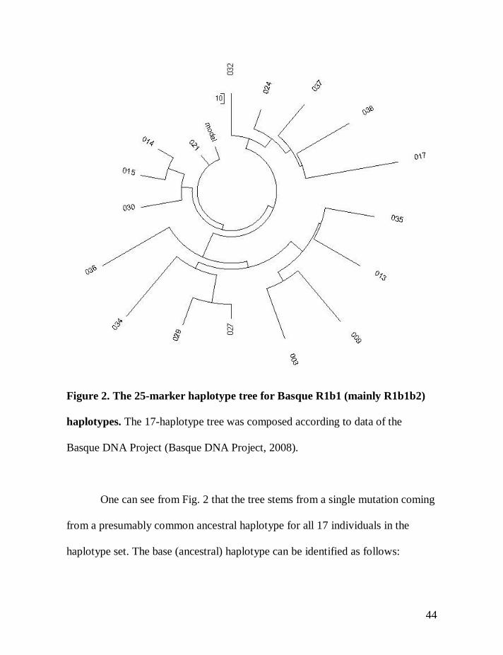
Figure 2. The 25-marker haplotype tree for Basque R1b1 (mainly R1b1b2)

haplotypes. The 17-haplotype tree was composed according to data of the

Basque DNA Project (Basque DNA Project, 2008).

One can see from Fig. 2 that the tree stems from a single mutation coming

from a presumably common ancestral haplotype for all 17 individuals in the

haplotype set. The base (ancestral) haplotype can be identified as follows:

45

13-24-14-11-11-14-12-12-12-13-13-29-17-9-10-11-11-25-14-18-29-15-15-17-17

In fact, this is the haplotype 021 on the tree (Fig. 2) and in the list of haplotypes

above. However, one base haplotype is not enough to use the logarithmic

approach, since it can be just an accidental match. A rule of thumb tells that there

should be at least 3-4 base haplotypes in a series in order to consider the

logarithmic method.

In the 12-marker format the Basque ancestral haplotype is also identical to

the so-called Atlantic Modal Haplotype (Klyosov, 2008a, 2008b).

13-24-14-11-11-14-12-12-12-13-13-29

The “linear” method. All 17 of 25-marker haplotypes have 100

mutations from the above base (ancestral) haplotype (DYS389-1 was subtracted

from DYS389-2), which gives 0.235±0.024 mutations per marker on average (the

statistical treatment of the data is given below). Using Tables 1 and 2, one can

calculate a time span to a common ancestor of the Basques presented in the

haplotype set, which is equal to 147±21 generations, or 3,675±520 years.

Using the same approach for all 44 of 12-marker Basque R1b1b2

haplotypes, one finds that all of them contain 122 mutations from the base

haplotype

46

13-24-14-11-11-14-12-12-12-13-13-29

which corresponds to 0.231±0.021 mutations per marker on average, 145±20

generations or 3,625±490 years to a common ancestor. It is practically equal to

the findings above of 3,675±520 years obtained from the 25-marker set of

haplotypes.

However, these calculations are applicable only for symmetrical

mutations over the whole haplotype series, which does not exactly apply in the

considered case since the mutations were asymmetrical: 65 of single mutations

were “up” and only 36 “down”, all three double mutations were up, and all five

triple mutations were down. The degree of asymmetry for 12-marker haplotypes

equals to 0.64, hence, a = 0.0784, a1 = 0.869, and an average number of mutations

per marker, corrected for reverse mutations, calculated by using formula (1), is

equal to 0.257±0.023 .

Thus, the “linear” method ( obs = 0.231±0.021); the same method,

corrected for back mutations assuming a symmetrical pattern of mutations and

using Table 2 ( = 0.265±0.024); and corrected for back mutations and

asymmetry of the mutations ( = 0.257±0.023) results, respectively, in 145±20

and 140±19 generations, or 3625±490 and 3500±470 years to a common

ancestor.

47

Here, the degree of asymmetry of 0.64, that is about two thirds of “one-

sided” mutations, resulted in a slightly increased TSCA, if the respective

correction is not made. The increase in this particular case was 5 generations on

average, or 3.6% of the total. The increase progressively grows with the “age” of

the common ancestor.

The standard deviation, calculated by using formula (4), gives

095.0)2257.0869.01(

257.05281)(

that is 9.5%. It results in 3,500±170 years to a common ancestor, without

considering an error margin for the average mutation rate. If a standard deviation

for the last one is about 5%, it gives the overall SD of %8.13105.9 22 for

the 95% confidence interval, that is 3,500±480 years to a common ancestor of the

given Basque series of haplotypes.

The Chandler’s mutation rates (see above) results in 0.231/0.00187 = 124

generations (12-marker haplotypes) and 0.235/0.00278 = 85 generations (25-

marker haplotypes) to the common ancestor of the Basque haplotypes (the

standard deviations are omitted here). Obviously, there is significant mismatch

between the two values (46% difference). The difference increases even more

when the necessary correction for back mutations is introduced from Table 2. It

48

results in 142 and 93 generations, respectively, to the common ancestor, with

53% difference between the two values.

One can notice that for 12-marker haplotypes the values of 145 (our data)

and 142 (Chandler’s data) generations to a common ancestor are practically

identical. However, it is a series of 25-marker haplotypes which does not fit the

Chandler’s mutation rates but nicely corresponds to the mutation rates employed

in this work.

We can also test the Kerchner’s mutation rates, which would result in

0.231/0.0025 = 92 generations and 0.235/0.0028 = 84 generations, for 12- and

25-marker series, respectively, that is 102 and 92 generations after correction for

back mutations. For 25 years per generation it would give 2550 – 2300 years to

the Basque common ancestor, which is an unbelievably recent time period (but

who knows?). Even at 35 years per generation, which for ancient people would be

probably a stretch, it still gives 3570 – 3,220 years bp, the latter figure for

(supposedly) more accurate 25-marker haplotypes.

ASD methods. In order to verify the obtained timespan to a common ancestor

and validity of the correction for reverse mutations, we have employed the

average square distance (ASD) method in its two principal variants –

(a) employing a base (ancestral) haplotype, and (b) without a base haplotype, that

is employing permutations of all alleles (Adamov & Klyosov, 2008b). Both of the

49

ASD methods do not need to include corrections for back mutations, but they are

more tedious otherwise, when used manually. Besides, the variant (a) is sensitive

to asymmetry of mutations in the series (Adamov & Klyosov, 2008b, 2009a), and

particularly to even a small amount of extraneous haplotypes. Both the ASD

methods typically give a higher error margin compared with the “linear” method,

commonly as a result of multiple (multi-step) mutations and accidental

admixtures of haplotypes from a different common ancestor (Adamov &

Klyosov, 2009a).

The ASD method, using the base haplotype. Since all 44 of 12-marker

haplotypes contain 101 single-step mutations, three double mutations, and five

triple mutations, the “actual” number of mutations in the 44-haplotype set is 101

+ 3x22 + 5x32 = 158. The observed number of mutations was 122 (see above), or

77% of the actual, as the calculations showed. Hence, an average number of

actual mutations per marker is 0.299±0.027 (compared to the observed

0.231±0.021, see above), which corresponds to 163±22 generations or 4,075±550

years to a common ancestor. It overlaps with the 3500±470 ybp obtained with the

“linear” method, in the margin of error range, which should be slightly higher for

the ASD-based figure due to a higher sensitivity of “quadratic” method to

admixtures as well as to double and triple mutations in the haplotype series (there

50

are three double and five triple mutations in the 12-marker haplotype series,

hence, the higher “age” of the series calculated by ASD).

The permutational ASD method, no base haplotype. We will illustrate

this method using 25-marker haplotypes. There are 17 alleles for each marker in

the haplotypes, and the method considers permutations between each one of

them, with squares of all the differences summed up for all the 25 markers. For

17 Basques haplotypes this value equals to 3728. It should be divided by 172 (all

haplotypes squared), then by 25 (a number of markers in a haplotype) and by 2

(since all permutations are doubled by virtue of the procedure). This gives

0.258±0.035 as an average number of “actual” mutations per marker, which

corresponds to 141±19 generations to a common ancestor. It is remarkable that it

practically equals to 0.257±0.023 as the respective figure for the 44 of 12-marker

haplotypes, corrected for back mutations and asymmetry of the mutations, and

shows how accurate calculations can be when justified approaches are employed.

In summary, the linear method gave 145±20 and 140±19 generations to a

common ancestor (with and without correction for asymmetry of mutations), the

ASD/base haplotype gave 163±22 generations, and the ASD/permutational gave

141±19 generations to a common ancestor. All results are in a reasonably good

agreement with each other, with the ASD/base-generated figure 12-16% higher

than the other three. The most reliable figure is 3,500±480 years to a common

51

ancestor of present day Basques exemplified with the considered 44 haplotypes.

This value is on a lower side of European R1b1b2 common ancestor, and will be

discussed in the subsequent paper (Part II).

Iberian R1b1 19-marker haplotypes

In order to further verify the approach, 750 of 19-marker Iberian R1b1

haplotypes were considered. The haplotype tree, based on the published data

(Adams et al, 2008) is given in Fig. 3, with a purpose to show that the tree is a

pretty uniform, reasonably symmetrical, and does not contain ancient, distinct

branches. All branches are of about the same length. This all indicates that the

tree, with its most or all of the 750 haplotypes, is derived from a relatively recent

common ancestor, who lived no more than four or five thousand years ago. It

would be impossible for the tree to be derived from a common ancestor who lived

some 10-15 years ago, much less 30 thousand years ago.

Let us verify it.

First, the base haplotype for all the 750 entries, obtained by a

minimization of mutations, in the format DYS 19-388-3891-3892-390-391-392-

393-434-435-436-437-438-439-460-461-462-385a-385b, employed by the

authors (Adams et al, 2008), is as follows:

52

14-12-13-16-24-11-13-13-11-11-12-15-12-12-11-12-11-11-14

In this format the Atlantic Modal Haplotype (AMH) is as follows (Klyosov,

2008a):

14-12-13-16-24-11-13-13- X- X- Y- 15-12-12-11- X- X- 11-14

in which X replaces the alleles which are not part of the 67-marker FTDNA

format, and Y stands for DYS436 which is uncertain for the AMH. The same

haplotype is the base one for the subclade U152 (R1b1c10), with a common

ancestor of 4375 ybp, and for R1b1b2 haplogroup with a common ancestor of

4450 ybp (Klyosov, 2008a). Hence, the Iberian R1b1 haplotypes is likely to have

a rather recent origin.

53

Figure 3. The 19-marker haplotype tree for Iberian R1b1 haplotypes. The

tree was composed according to data published (Adams et al, 2008).

All 750 haplotypes showed 2796 mutations with respect to the above base

haplotype, with a degree of asymmetry of 0.56. Therefore, the mutations are

54

fairly symmetrical, and a correction for the asymmetry would be a minimal one.

The whole haplotype set contains 16 base haplotypes.

An average mutation rate for the 19-marker haplotypes is not available in

the literature, as far as I am aware of, and cannot be calculated using the

Chandler’s, Kerchner’s, or other similar data. However, the Donald Clan latest

edition of 88 haplotypes contains 63 mutations in the above 19 markers. Taking

into account the 26 generations to the Clan founder (see above), this results in the

mutation rate of 0.0015 mut/marker/gen and 0.0285 mut/haplotype/gen, listed in

Table 1.

The logarithmic method gives ln(750/16)/0.0285 = 135 generations, and a

correction for reverse mutations results in 156 generations (Table 2), that is 3900

years to a common ancestor of all the 750 Iberian 19-marker haplotypes. It

corresponds well with 3500±480 ybp value, obtained above for 12- and 25-

marker haplotype series. The “mutation count” method gives 2796/750/19 =

0.196±0.004 mutations per marker (without a correction for back mutations, that

is obs = 0.196±0.004), or after the correction it is of 0.218±0.004 mutations per

marker, or 0.218/0.0015 = 145±15 generations, that is 3625±370 years to a

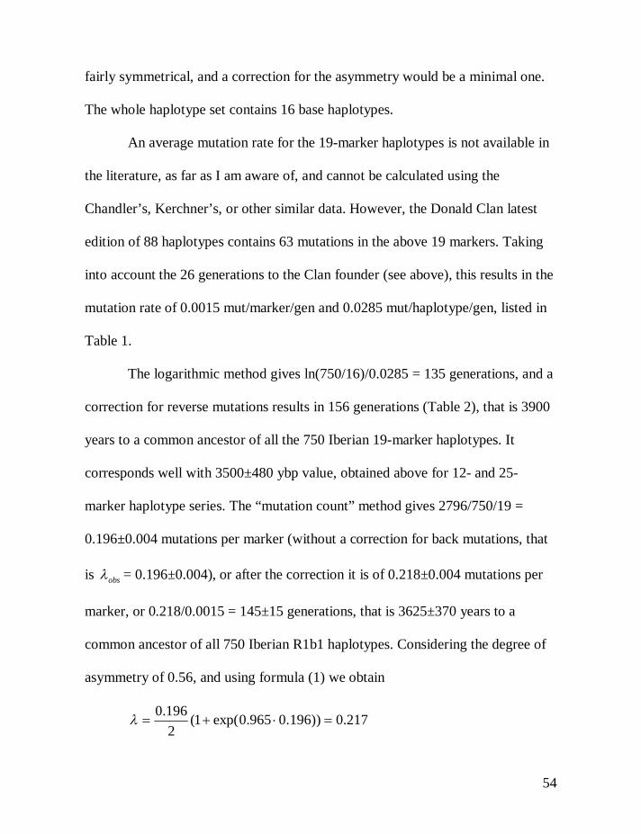
common ancestor of all 750 Iberian R1b1 haplotypes. Considering the degree of

asymmetry of 0.56, and using formula (1) we obtain

217.0))196.0965.0exp(1(2196.0

55

In other words, at the degree of asymmetry of 0.56 the average number of

mutations per marker, 0.217±0.004, is practically equal to 0.218±0.004 for the

fully symmetrical (ε = 0.50) pattern of mutations in the haplotype series. It gives

145±15 generations, that is 3625±370 years to a common ancestor. Formula (4)

gives the standard deviation

)2

196.0965.01(196.014250

1)(

= 2% (5)

that is 0.217±0.004 mut/marker, and for the 5% standard deviation for the

mutation rate, the 95% confidence interval for the time span to a common

ancestor with be equal to %2.10102 22 . This is how the above figure of

3625±370 ybp for the 750 Iberian 19-marker haplotypes was calculated. This

figure is practically equal to 3,500±480 ybp for 12- and 25-marker Basque

haplotypes.

It might look that the margin of error of 2.0% is too low, even for 750 19-

marker haplotypes, with a total 14,250 alleles. In fact, it is not too low. For a

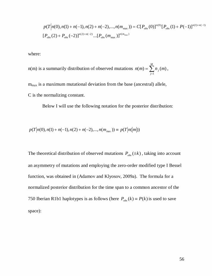
verification of formula (4) we obtain the Bayesian posterior distribution for the

time T to the TSCA, as it was obtained by Walsh (Walsh, 2001) and applied in

(Adamov and Klyosov, 2009b) with a consideration of the asymmetry of a

haplotype series:

56

)(max

)2()2(

)1()1()0(max

max)](...[)]2()2([

)]1()1([)]0([))(),...,2()2(),1()1(),0((mn

obsnn

obsobs

nnobs

nobs

mPPP

PPPCmnnnnnnTp

where:

n(m) is a summarily distribution of observed mutations

M

jj mnmn

1)()( ,

mmax is a maximum mutational deviation from the base (ancestral) allele,

C is the normalizing constant.

Below I will use the following notation for the posterior distribution:

))(())(),...,2()2(),1()1(),0(( max mnTpmnnnnnnTp

The theoretical distribution of observed mutations )( kPobs , taking into account

an asymmetry of mutations and employing the zero-order modified type I Bessel

function, was obtained in (Adamov and Klyosov, 2009a). The formula for a

normalized posterior distribution for the time span to a common ancestor of the

750 Iberian R1b1 haplotypes is as follows (here )()( kPkPobs is used to save

space):

57

0

239137239711675

239137239711675

)]4()4([)]3()3([)]2()2([)]1()1([)]0([

)]4()4([)]3()3([)]2()2([)]1()1([)]0([))((dTPPPPPPPPP

PPPPPPPPPmnTp

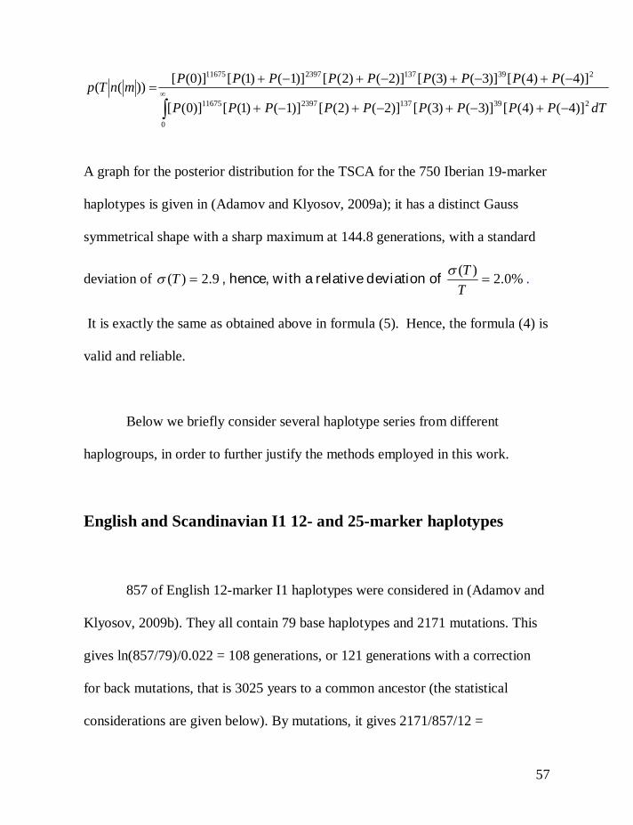
A graph for the posterior distribution for the TSCA for the 750 Iberian 19-marker

haplotypes is given in (Adamov and Klyosov, 2009a); it has a distinct Gauss

symmetrical shape with a sharp maximum at 144.8 generations, with a standard

deviation of 9.2)( T , hence, with a relative deviation of %0.2)(

TT .

It is exactly the same as obtained above in formula (5). Hence, the formula (4) is

valid and reliable.

Below we briefly consider several haplotype series from different

haplogroups, in order to further justify the methods employed in this work.

English and Scandinavian I1 12- and 25-marker haplotypes

857 of English 12-marker I1 haplotypes were considered in (Adamov and

Klyosov, 2009b). They all contain 79 base haplotypes and 2171 mutations. This

gives ln(857/79)/0.022 = 108 generations, or 121 generations with a correction

for back mutations, that is 3025 years to a common ancestor (the statistical

considerations are given below). By mutations, it gives 2171/857/12 =

58

0.211±0.005 mut/marker ( obs , without a correction), or 0.238±0.005 mut/marker

(corrected for back mutations), or 0.220±0.005 (corrected for back mutations and

the asymmetry of mutations, which equal to 0.87 in this particular case). This

results in 0.220/0.00183 = 120±12 generations to a common ancestor. This is

practically equal to the 121 generations, obtained by the logarithmic method.

Obviously, the logarithmic method, being irrelevant to asymmetry of mutations

(since only base, non-mutated haplotypes are considered), can be preferred

method in cases of high asymmetry of mutations. This results in 3,000±300 years

to a common ancestor for all the 857 English 12-marker haplotypes.

The asymmetry of mutations, which is rather high in this particular case

(0.87) adds 10 generations (250 years) to the TSCA, corrected for reverse

mutations. This addition was properly corrected back in this particular case.

The same haplotypes, but in the 25-marker format, contain 4863

mutations, which gives obs = 0.227±0.003 mut/marker, and = 0.260±0.004

(corrected for back mutations), and = 0.251±0.004 (corrected for both back

mutations and asymmetry of mutations). It is of interest that for 25-marker

haplotypes the degree of asymmetry was appreciably lower, 0.66 compared to

0.87 for 12-marker haplotypes. This gives 0.251/0.00183 = 137±14 generations,

that is 3,425±350 years to a common ancestor. The difference between the

TSCA’s for 12- and 25-marker series equals to 14±2%. The reasonably low

degree of asymmetry (0.66) added only 5 generations, that is 125 years, to the

59

TSCA, corrected only for back mutations. This is only 3.6% in this particular

case, however, progressively grows when the TSCA is much “older”.

The Chandler’s mutation rates would result in 0.220/0.00187 = 118

generations for the 12-marker series, and 0.251/0.00278 = 90 generations for the

25-marker series. The difference is 31% (!).

The Kerchner’s mutation rates would give 88 and 90 generations, which is

an excellent fit. It gives the time spans of 2200 and 2250 ybp, which is 36-52%

lower compared to the estimates of this work. This was expected, since the

Kerchner’s rates resulted in reduced values of TSCA for the Donald Clan

haplotype series.

If to combine the above 857 English I1 haplotype series with 366 Irish I1

haplotypes and 304 Scottish I1 haplotypes, the resulted 1527 of 25-marker

haplotypes contain 8785 mutations, obs = 0.230±0.002 mut/marker, =

0.265±0.003 (corrected for back mutations), and = 0.255±0.003 (corrected for

both back mutations and asymmetry of mutations). Again, in this combined

haplotype set the degree of asymmetry was higher for 12-marker haplotypes:

0.85, compared to 0.65 for 25-marker haplotypes. This results in 0.255/0.00183 =

139±14 generations, that is 3475±350 years to a common ancestor. This is

practically equal to the TSCA for the English haplotypes (3425±350 ybp).

The standard deviations for the 1527 25-marker haplotype series were

calculated using formula (4) which gives “two sigma” in this particular case as

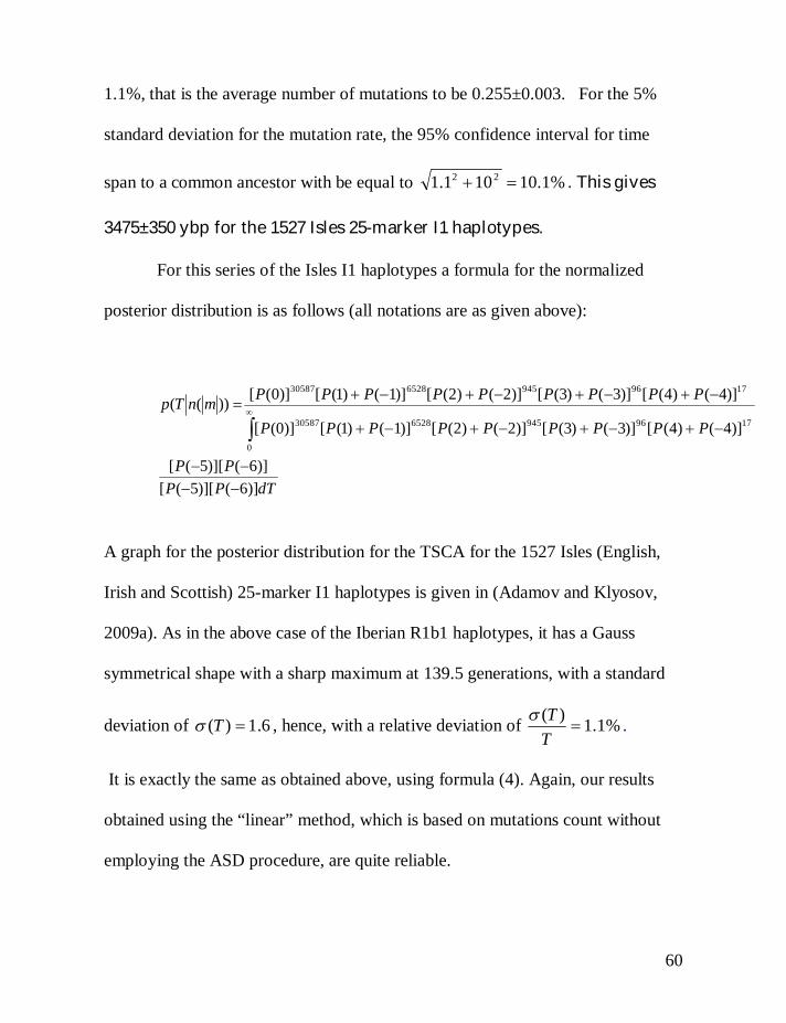
60

1.1%, that is the average number of mutations to be 0.255±0.003. For the 5%

standard deviation for the mutation rate, the 95% confidence interval for time

span to a common ancestor with be equal to %1.10101.1 22 . This gives

3475±350 ybp for the 1527 Isles 25-marker I1 haplotypes.

For this series of the Isles I1 haplotypes a formula for the normalized

posterior distribution is as follows (all notations are as given above):

dTPPPP

PPPPPPPPP

PPPPPPPPPmnTp

)]6()][5([)]6()][5([

)]4()4([)]3()3([)]2()2([)]1()1([)]0([

)]4()4([)]3()3([)]2()2([)]1()1([)]0([))((

0

1796945652830587

1796945652830587

A graph for the posterior distribution for the TSCA for the 1527 Isles (English,

Irish and Scottish) 25-marker I1 haplotypes is given in (Adamov and Klyosov,

2009a). As in the above case of the Iberian R1b1 haplotypes, it has a Gauss

symmetrical shape with a sharp maximum at 139.5 generations, with a standard

deviation of 6.1)( T , hence, with a relative deviation of %1.1)(

TT .

It is exactly the same as obtained above, using formula (4). Again, our results

obtained using the “linear” method, which is based on mutations count without

employing the ASD procedure, are quite reliable.

61

Speaking of the ASD, or the “quadratic” method, it is worth mentioning

that it gave the following values for the average number of mutations per marker

for the 12- and 25-marker 1525-haplotype Isle combined series: 0.244±0.015 and

0.296±0.038, that is 133±16 and 162±26 generations, respectively, compared to

124±12 and 139±14 generations to the common ancestor, and to 139.5

generations obtained by using the Bayesian posterior distribution for the 25-

marker haplotypes. For this particular series of haplotypes the ASD procedure

results in a higher margin of error for the average number of mutations per

marker (the “two sigma” was 6-12% compared to 1-2% for the “linear” method),

hence, in slightly elevated figures (typically by 15-20% in the TSCA for 25-

marker haplotypes) due to multiple mutations and possible extraneous

haplotypes.

Discussion

There is a number of typical questions and issues addressed when the very basis

of quantitative DNA genealogy is considered. Among them are the following

ones:

1) Which mutations should be counted and which should be not?

The underlying reason is that there is a potential problem of counting the same

mutation multiple times. For example, in Fig. 2 one can see three branches, each

stemming from a supposedly one ancestral (base) haplotype. The branch at the

62

bottom of the Figure contains eight haplotypes with the distinct common DYS437

= 15, while all other branches contain 14 in that locus. Hence, the typical

argument is that the common ancestor of this branch had DYS437 = 15, and this

very mutation (one step from the AMH) was counted eight times (in fact, nine

times, since 036 contains there 16). Therefore, as opponents argue, one probably

over-counts the mutations, and obtains an erroneously high number of

generations to the common ancestor of the entire haplotype set.

Generally, this consideration may be valid (see below), but not in this

particular case. First, as it was shown above, the same number of generations to

the common ancestor was obtained from both 12-marker haplotypes (which do

not include DYS437), using both the logarithmic and the “linear” methods, also

from the 25-marker haplotypes, and from a large series of 19-marker haplotypes.

However, there is another way to examine the obtained value, namely, to consider

all the three branches in Fig. 2. The branch at the bottom contains eight

haplotypes, all contain 46 mutations from its common ancestor of the branch,

which gives 144±26 generations from the common ancestor of the branch. The

five-haplotype upper-right branch contains 16 mutations, which gives 75±19

generations to its common ancestor. The three-haplotype upper-left branch

contains only 5 mutations from its base haplotype, which gives 39±17

generations to its common ancestor. An average number of generations for all

63

three branches is 86±21. Certainly, these operations are very approximate ones,

and they aim at the semi-quantitative verification of the concept.

Then we apply the same approach to those three base haplotypes as

described above. They all have 8 mutations between them from the base

haplotype for the entire haplotype series, which results in summarily 62±6

generations from the common ancestor for the whole series to the “averaged”

common ancestor of the separate branches. This gives (86±21)+(62±6) = 148±27

generations from the initial common ancestor to the present time, .

This figure is pretty close to 147±21 generations obtained by the “linear”

method (see above). Indeed, mutations in haplotypes can be considered as

practically independent ones, and we can count them either for the entire

haplotype series, provided that all haplotypes are derived from one common

ancestor, or analyze branches separately, as it was shown above.

In many cases one indeed can over-count mutations, particularly when

they belong to different branches and to different common ancestors. For

example, English and Irish R1a1 haplotype series contain many DYS388 = 10 (in

one particular haplotype series of 57 English haplotypes there are 10 of them, and

in 52 Irish haplotypes there are 12 of them, that is 18% and 23%, respectively).

There are practically no such DYS388=10 alleles in Polish, Czech, Slovak,

Hungarian, Russian, Jewish and Indian R1a1 haplotypes, and very few among

Swedish and German haplotypes. Incidentally, there was not a single case of

64

DYS388=10 in R1b1 haplotype series considered in the subsequent paper (Part

II), containing 750 Iberian, and 983 and 218 Irish haplotypes. DYS388 is an

extremely slow marker, and it is likely that all R1a1 haplotypes with DYS388=10

descended from the same, just one common ancestor.

When mutations in R1a1 haplotypes are counted assuming that

DYS388=10 is a common, random mutation, without a consideration that those

haplotypes are derived from a different common ancestor, each DYS388 = 10

haplotype adds a double mutation, which is particularly damaging when the ASD

method is employed. On a haplotype tree of English and Irish R1a1 haplotypes

the DYS388 = 10 branches stand out quite distinctly (the trees are shown in the

subsequent paper, Part II). If to count all those double mutations, without

separation the branches, the Irish “phantom” common ancestor comes out as of

5000 ybp. However, a separate consideration of the branches results in 3575±450

ybp for the DYS388 = 10 common ancestor, and in 3850±460 ybp for the

DYS388 = 12 common ancestor. However, their 25-marker base haplotypes

differ by six mutations, which places their common ancestor at 5,700±600 years

before present (see Part II).

Another remarkable example of a potential over-count of mutations is

related to haplotypes with DYS426 = 10 in haplogroup J1. It is known that

DYS426 is an extremely slow marker. Those mutations are so infrequent that

they are practically irreversible. In haplogroups of an earlier origin, including C

65

through O, a great majority of people have DYS426 = 11. Only in “younger”

haplogroups, Q and R, a great majority of people have DYS426 = 12. For

example, among all 343 haplotypes of haplogroup J1 in YSearch, collected in

2008, only 23 had DYS426 = 10 or 12. It turned out that all of them derived from

one common ancestor each, and in fact the same mutation was carried through

practically all the generations in the respective lineage over many thousand years.

Fig. 4 shows the 12-marker J1 haplotype tree with mutated DYS426.

Haplotypes of all said 23 individuals are shown there. Of all the 23 haplotypes,

eleven are located in the vicinity of the “trunk” of the tree, and eight of their

bearers have Jewish surnames (haplotypes 002 through 006, 008, 010 and 011 in

Fig. 4). They have five base haplotypes and four mutations among those eight,

which gives ln(8/5)/0.022 = 21 generations, and 4/8/0.022 = 23±12 generations,

that is 550±200 years to their common ancestor, who lived, apparently, around

the 15th century, and had the following haplotype:

12-24-13-10-12-19-10-15-13-12-11-29

Other eight individuals with DYS426 = 10 did not have typical Jewish surnames.

They had the following base haplotype:

12-24-13-10-12-19-10-15-12-12-11-29

66

All those 8 haplotypes had 24 mutations, which brings their common ancestor to

3950±1450 ybp.

Figure 4. The 12-marker haplotype tree for J1 haplotypes with mutated

DYS426. The tree was composed from haplotypes collected in YSearch data

base. Bearers of haplotypes 002, 003, 004, 005, 006, 008, 010 and 011 have

Jewish surnames.

67

Haplotypes of the remaining seven individuals had DYS426 = 12, and form a

distinct, obviously very ancient branch on the right-hand side in Fig. 4. Most of

them have rather typical European surnames, along with one Palestinian

individual among them. Their deduced base haplotype:

12-24-14-10-12-14-12-13-12-13-11-29

All the seven haplotypes contained 46 mutations from this base haplotype, which

indicates that their common ancestor lived 10600±1900 years ago.

The above and the “Jewish” J1 haplotypes differ by 12 mutations on 12-

markers, which brings their common ancestor to 760±135 generations ago, that is

19,000±3,400 ybp. This is as close to the “bottom” of J1 haplogroup as one gets.

These examples show that in order to avoid over-count of mutations one

should consider a haplotype tree, separate branches, and calculate them

separately.

2) Which mutation rates to use?

This question was considered in details in (Athey, 2007). He specifically

considered three sets of mutation rates, those advanced by Chandler, Kerchner

68

and Zhivotovsky. The first two are similar in kind, though based on different

sources of haplotypes. For the first three panel of markers in the FTDNA format

the respective mutation rates are 0.00187±0.00028, 0.00278±0.00042, and

0.0492±0.00074 (Chandler), 0.0025±0.0003, 0.0028±0.0002, and 0.0043±0.0002

(Kerchner) compared to the rates employed in this work (0.00183±0.00009,

0.00183±0.00009, and 0.00243±0.00024) [Table 1]. I have tested all the three

mutation rate sets with multiple haplotype systems, and some results are shown

above. Overall, I came to a conclusion that the set of mutation rates employed in

this work (Table 1) is the most agreeable with actual haplotype series, and gives

the most consistent results between 12-, 25-, and 37-marker haplotypes and with

expected time spans to common ancestors.

Here is an example, one of many. It is related to a rather recent common

ancestor. A reader sent me a 25-marker haplotype set of eight relatives in Britain.

He asked me to determine when a common ancestor lived, however, did nor

disclose the actual date. The list was as follows:

13 25 14 10 11 14 12 12 10 13 11 30 15 9 10 11 11 23 14 20 35 15 15 15 16

13 25 15 10 11 14 12 12 10 13 11 29 15 9 10 11 11 23 14 20 35 15 15 15 16

13 25 15 10 11 14 12 12 10 13 11 30 15 9 9 11 11 23 14 20 35 15 15 15 15

13 25 15 10 11 14 12 12 10 13 11 30 15 9 10 11 11 23 14 20 35 15 15 15 16

13 25 15 10 11 14 12 12 10 13 11 30 15 9 10 11 11 23 14 20 35 15 15 15 16

69

13 25 15 10 11 14 12 12 10 13 11 30 15 9 10 11 11 23 14 20 35 15 15 15 16

13 25 15 10 11 14 12 12 10 13 11 30 15 9 10 11 11 23 14 20 35 15 15 15 16

13 25 15 10 11 14 12 12 10 13 11 30 15 9 10 11 11 23 14 20 35 15 15 15 16

Clearly, the base, ancestral haplotype is as follows:

13 25 15 10 11 14 12 12 10 13 11 30 15 9 10 11 11 23 14 20 35 15 15 15 16

All eight haplotypes have three mutations per 200 alleles. It gives

3/8/0.046 = 8 generation from a common ancestor. At the same time the series

contains five base haplotypes, which gives ln(8/5)/0.046 = 10 generations. It

gives the average value of 9±1 generation. However, formula (4) shows that for a

200-marker series and three mutations in it, for a fully asymmetrical mutations

(which the series has) a standard deviation theoretically equals to 57.7%. At the

68% confidence level (“one sigma”, the 5% standard deviation for the mutation

rate) we obtain that there would be 9±3 generations, and at the 95% confidence

level (“two sigma”, the 10% standard deviation for the mutation rate) there would

be 9±5 generations to the common ancestor. Therefore, the common ancestor

lived in 1784±75 (68% confidence), or in 1784±125 (95% confidence). In fact, as

I was informed, Robert, the common ancestor of all the eight individuals, was

born in 1767. His son, also Robert, was born in 1797.

70

Zhivotovsky “evolutionary” mutation rate of 0.00069 mutations per

marker per generation was empirically derived using a number of questionable

assumptions, and it was recommended for use not in “genealogical”, or

“pedigree-based”, but in “population dynamics” studies. Criteria of when a series

of haplotypes represent the “population” and when “genealogical” situation were

not provided. As a result, this mutation rate have been widely used in the

academic literature quite indiscriminately, often (or always) resulting in time

spans to common ancestors some 300-400% higher compared to those obtained

with “genealogical” mutation rates.

In fact, it is easy to calculate from Table 2 that the 0.00069 mut/mark/hapl

mutation rate is applicable for a time span equal to 2560 generations, that is

64,000 years ago, no more, no less. For >64,000 ybp the actual mutation rate will

be lower than 0.00069, for <64,000 ybp the actual mutation rate will be higher

than 0.00069.

3) Are the same mutation rates applicable to the cases where the time

depth is a few hundred years, and where it is over a thousand or more years?

As it was shown in this study, the same mutation rates are well applicable

in the both cases, from as recent times as a couple of centuries to 3625±370 ybp

(the Basques and R1b Iberian haplotypes), and to 16,300±3,300 years (Native

71

Americans of Q-M3 haplogroup, see the subsequent paper) and there is no reason

to believe that they cannot be applicable to a much deeper time spans.

An illustration can be provided with a recent publication (Tofanelli et al,

2009), in which the authors listed 282 of 20-marker haplotypes of haplogroup J1-

M267. The authors gave an overall estimate of the “median TMRCA” between

6643 and 47439 ybp. Their list of 282 haplotypes showed a base haplotype (in the

format DYS 19-3891-3892-390-391-392-393-385a-385b-437-438-439-456-458-

635-GATAH4-YCAIIa-YCAIIb)

14-23-13-17-10-11-12-13-19-17-14-10-11-20-15-18-21-11-22-22

All the 282 haplotypes have 2746 mutations from that base haplotype,

which gives the average number of mutations per marker of 0.487±0.009, and the

TSCA of 6,025±610 years bp. In order to verify this figure, the tree (Fig. 5) was

subdivided to seven major branches, and the TSCAs were calculated to each of

them. Surprisingly, except the “oldest” branch in the upper right area with the

TSCA of 5,300±600 years, all other branches are relatively young, with the

youngest one in the middle left area, with TSCA of 1800±230 years, beginning of

the AD. Overall, the analysis of the branches showed that the common ancestor

of all of them lived 5,400±800 ybp. There is no reason to believe that calculations

72

of the TSCA work only at depths no more than a few hundred of years ago, even

with a rather complicated haplotype trees.

Another support to this statement is provided with a calculation of a time

span to the common ancestor of a few dozen haplotypes of haplogroup A, which

came out as about 75,000 ybp (to be published). There is nothing unexpected in

this figure. Clearly, in order to handle such distant time spans the tree should be

dissected to separate branches, and corrections for back mutations should be

applied.

73

Figure 5. The 20-marker haplotype tree for J1-M267 haplotypes. The tree

contains 282 haplotypes, and was composed according to data published

(Tofanelli et al, 2009).

74

4) How one can take the mutational analysis seriously, since the

standard deviations must be so high?

Such a general misconception is propagated mainly as a result of a non-

critical analysis of the well known paper by Walsh (2001). In his excellent paper

Walsh considered pairs of haplotypes, since the main goal was to provide a basis

for forensic analysis. Naturally, with only two haplotypes an error margin would

be huge, as follows from formula (4) above. For example, for two of 12-marker

haplotypes having a common ancestor 600 years ago the formula in its simplified

form (for a fully asymmetrical mutations and fully symmetrical mutations,

respectively)

042.0241)(

)2042.01(

042.0241)(

gives the margin of errors of 100%. The standard deviation of the mutation rate

will be added on top of it, however, it will not add much.

The same results will be observed if two 12-marker haplotypes (which

belong to the same haplogroup or a subclade) contain one mutation between

75

them. Then for the 68% confidence interval the common ancestor of these two

haplotypes lived between 1,140 ybp and the present time, and for the 95%

confidence interval he lived between 1,725 ybp and the present time.

A similar in kind situation will be observed for two, three or four

mutations between two 12-marker haplotypes in the FTDNA format. At the 95%

confidence level the common ancestor of the two individuals would have lived

between 2,900 ybp, or 3625 ybp, or 4575 ybp, respectively, and the present time,

even when the mutation rate is determined with the 5% accuracy.

Only with five mutations between two 12-marker haplotypes it is unlikely

– with the 95% confidence level – that the common ancestor lived within 12

generations, that is 300 years before present. It rather lived between 5500 ybp and

300 ybp.

Obviously, we have considered quite different situations, typically with

multiple haplotype series, which progressively reduce the standard deviations of a

number of average mutations per marker, in some cases with hundreds or even

well over a thousand of 25-marker haplotypes, down to 2.0% (with 750 of 19-

marker haplotypes) and 1.1% (with 1527 of 25-marker haplotypes, collectively

having almost 40 thousand alleles). In those cases the standard deviation of a time

span to a common ancestor is determined by only that for the mutation rate.

However, relative values of TSCA’s will stay with a reasonably good accuracy.

76

5) What are limitations of the logarithmic method of determining of a

time span to a common ancestor?

The logarithmic method has a firm basis, well proven in chemical

kinetics. The limitations are practically the same as there, though in chemical

kinetics nobody questions a validity of the method. It is commonly applied to

kinetics of the first order, which principally is the way how mutations appear in

the respective loci, that is statistically and without a direct influence of other

reagents, except the respective enzyme (a collective term here), a catalyst. In this

work it is applied to the amount of non-mutated, or base haplotypes, which

disappear in accord with the mutation rate. The faster the mutation rate, the faster

base haplotypes disappear from the haplotype series. For 12-, 25-, 37- and 67-

marker haplotypes, half of base haplotypes will disappear (become mutated) after

32, 15, 8, and 5 generations, respectively. Clearly, for 37- and 67-marker

haplotypes the logarithmic method is hardly applicable. For large series of 25-

marker haplotypes it can be quick and convenient. For example, in a series of 200

of 25-marker haplotypes, even after 65 generations, that is 1625 years, as many as

10 base haplotypes will still be present. This can easily be seen from

ln(200/10)/0.046 = 65 generations. For 12-marker haplotypes ln(200/10)/0.022 =

136, that is 10 base haplotypes in the series will still stay after about 3400 years.

To use the logarithmic method is not recommended when less than 4-5

base haplotypes present in the haplotype series.

77

A concern that a considerable data is discarded in order to focus on

unmutated haplotypes is a non-issue, since this method is recommended to be

applied along with the traditional method of mutation counting. Only when the

two methods give similar results (in terms of a number of generations or years to

the common ancestor), the results are justified. If the results are significantly

different, such as by 1.4-2 times or higher, neither of the results can be accepted.

A difference of 1.3-1.4 times is conditionally acceptable, however, results will

have a high margin of error.

Asymmetry of mutations

This phenomenon was considered in this study using a number of specific

examples. It was shown that when mutations are fairly symmetrical, that is both-

sided (the degree of asymmetry is around 0.5), no corrections to the TSCA are

needed. The TSCA is typically calculated as an average number of mutations per

marker, divided by the appropriate average mutation rate (Table 1) and corrected

for back mutations using Table 2. Alternatively, formula (1) can be employed in

its simplified version (with a1 = 1 for a symmetrical pattern of mutations). Even

when the degree of mutations reaches about 0.66 (two-thirds of mutations in the

haplotype series are one-sided), the respective correction is not significant and is

typically within a corresponding margin of error (for the Basque R1b1b2

78

haplotypes it was of 5 generations, that was 3.6% of total). For the degree of

asymmetry around 0.85 (as in the case of the Isles I1 haplotypes, considered

above) the necessary correction can be around 10-20 generations (250 years) on

the 120-generation span, that is reach 8-16%, and further increase with an “age”

of the TSCA. At a fully one-sided mutation pattern (the degree of asymmetry

equal to 1), it completely nullifies the correction for reverse mutations, hence, can

increase the calculated TSCA by 750 years at 4000 years and by 1200 years at

5000 years to the common ancestor, respectively, and continue to grow. This is,

of course, the extreme case of asymmetry, however, it should be taking into

consideration.

Overall, this section has essentially shown how to make calculations and

interpret data extracted from a number of mutations and a number of base

haplotypes in haplotype sets. The subsequent paper (Part II) will follow with

principal illustrations and conclusions, without repeating the methodology.

Acknowledgements I am indebted to Theresa M. Wubben and Dmitry Adamov

for valuable discussions, and to Dr. Whit Athey for multiple suggestions and

critical consideration of the manuscript.

79

References

Adamov, D.S., and Klyosov, A.A. (2008a). Theoretical and practical estimates of

reverse mutations in haplotypes of Y chromosome (in Russian). Proc. Russian

Academy of DNA Genealogy (ISSN 1942-7484), 1, 631-645.

Adamov, D.S., and Klyosov, A.A. (2008b). Evaluation of an “age” of populations

from Y chromosome using methods of average square distance (in Russian).

Proc. Russian Academy of DNA Genealogy (ISSN 1942-7484), 1, 855-905.

Adamov, D.S., and Klyosov, A.A. (2009a). Evaluation of an “age” of populations

from Y chromosome. Part I. Theory (in Russian). Proc. Russian Academy of DNA

Genealogy (ISSN 1942-7484), 2, 81-92.

Adamov, D.S., and Klyosov, A.A. (2009b). Practical methods for determining

“age” of common ancestors for large haplotype series (in Russian). Proc. Russian

Academy of DNA Genealogy (ISSN 1942-7484), 2, 422-442.

Adamov, D.S., and Klyosov, A.A. (2009c). Evaluation of an “age” of populations

from Y chromosome. Part II. Statistical considerations (in Russian). Proc.

Russian Academy of DNA Genealogy (ISSN 1942-7484), 2, 93-103.

80

Adams, S.M., Bosch, E., Balaresque, P.L., Ballereau, S.J., Lee, A.C., Arroyo, E.,

López-Parra, A.M., Aler, M., Gisbert Grifo, M.S. , Brion, M., et al. (2008) The

Genetic Legacy of Religious Diversity and Intolerance: Paternal Lineages of

Christians, Jews, and Muslims in the Iberian Peninsula. Amer. J. Hum. Genet, 83,

725-736.

Athey, W. (2007) Mutation rates – who’s got the right values?. J. Genet. Geneal.

3, (Editor’s Corner).

Basque DNA Project. URL : http://www.familytreedna.com/public/BasqueDNA,

2008.

Chandler, J.F. (2006). Estimating per-locus mutation rates. J. Genetic Genealogy

2, 27-33.

Cordaux, R., Bentley, G., Aunger, R., Sirajuddin, S.M., Stoneking, M. (2004) Y-

STR haplotypes from eight South Indian groups based on five loci. J. Forensic

Sci. 49, 1-2.

81

Cruciani, F., La Fratta, R., Trombetta, B., Santolamazza, P., Sellitto, D., Colomb,

E.B., Dugoujon, J.-M., Crivellaro, F., Benincase, T., Pascone, R. et al. (2007)

Tracing past human male movement in Northern/Eastern Africa and Western

Eurasia: new clues from Y-chromosomal haplogroups E-M78 and J-M12. Mol.

Biol. Evol. 24, 1300-1311

DNA-Project.Clan-Donald. URL: http://dna-project.clan-donald-

usa.org/tables.htm, 2008.

Felsenstein, J. (2005). Phylip, the Phylogeny Inference Package. PHYLIP,

version 3.6. Department of Genome Sciences, University of Washington, Seattle.

Goldstein, D.B., Linares, A.R., Cavalli-Sforza, L.L. and Feldman, M.W. (1995a).

Genetic absolute dating based on microsatellites and the origin of modern

humans. Proc. Natl. Acad. Sci. US, 92, 6723-6727.

Goldstein, D.B., Linares, A.R., Cavalli-Sforza, L.L. and Feldman, M.W. (1995b).

An evaluation of genetic distances for use with microsatellite loci. Genetics 139,

463-471.

82

Hammer, M.F., Redd, A.J., Wood, E.T., Bonner, M.R., Jarjabazi, H., Karafet, T.,

Santachiara-Benerecetti, S., Oppenheim, A., Jobling, M.A., Jenkins, T., et al.

(2000). Jewish and Middle Eastern non-Jewish populations share a common pool

of Y-chromosome biallelic haplotypes. Proc. Natl. Acad. Sci. US. 97, 6769-6774.

Heyer, E., Puymirat, J., Dieltjes, P., Bakker, E., and de Knijff, P. (1997).

Estimating Y chromosome specific microsatellite mutation frequencies using

deep rooting pedigrees. Human Mol. Genetics 6, 799-803

Jobling, M.A., and Tyler-Smith, C. (1995). Fathers and sons: the Y chromosome

and human evolution. TIG, 11, 449-456.

Karafet, T.M., Zegura, S.L., Posukh, O., Osipova, L., Bergen, A., Long, J.,

Goldman, D., Klitz, W., Harihara, S., de Knijff, P., et al. (1999). Ancestral Asian

source(s) of New World Y-chromosome founder haplotypes. Am. J. Hum. Genet.

64, 817-831.

Kayser, M., Roewer, L., Hedman, M., Henke, L., Hemke, J., Brauer, S., Kruger,

C., Krawczak, M., Nagy, M., Dobosz, T., et al (2000). Characteristics and

frequency of germline mutations at microsatellite loci from the human Y

83

chromosome, as revealed by direct observation in father/son pairs. Am. J. Hum.

Genet. 66, 1580-1588.

Kerchner, C. (2008) Y-STR haplotype observed mutation rates in surname

projects study and log, http://kerchner.com/cgi-kerchner/ystrmutationrate.cgi

Klyosov, A.A. (2008a). The features of the “West European” R1b haplogroup (in

Russian). Proc. Russian Academy of DNA Genealogy (ISSN 1942-7484), 1, 568-

629.

Klyosov, A.A. (2008b). Origin of the Jews via DNA genealogy. Proc. Russian

Academy of DNA Genealogy (ISSN 1942-7484), 1, 54-232.

Klyosov, A.A. (2008c). Basic rules of DNA genealogy (in Russian). Proc.

Russian Academy of DNA Genealogy (ISSN 1942-7484), 1, 252-348.

Klyosov, A.A. (2008d). Calculations of time spans to common ancestors for

haplotypes of Y chromosome (in Russian). Proc. Russian Academy of DNA

Genealogy (ISSN 1942-7484), 1, 812-835.

84

Klyosov, A.A. (2008e). Where Slavs and Indo-Europeans came from? (in

Russian). Proc. Russian Academy of DNA Genealogy (ISSN 1942-7484), 1, 400-

477.

Mertens, G. (2007) Y-Haplogroup frequencies in the Flemish population. J.

Genet. Geneal. 3, 19-25.

Mulero, J.J., Chang, C.W., Calandro, L.M., Green, R.L., Li, Y., Johnson, C.L.,

and Hennessy, L.K. (2006) Development and validation of the AmpFlSTR Yfiler

PCR amplification kit: a male specific, single amplification 17 Y-STR multiplex

system. J Forensic Sci 51, 64-75.

Nebel, A., Filon, D., Weiss, D.A., Weale, M., Faerman, M., Oppenheim, A., and

Thomas, M. (2000). High-resolution Y chromosome haplotypes of Israeli and

Palestinian Arabs reveal geographic substructure and substantial overlap with

haplotypes of Jews. Hum. Genet. 107, 630-641.

Nebel, A., Filon, D., Brinkmann, B., Majumder, P.P., Faerman, M., and

Oppenheim, A. (2001). The Y chromosome pool of Jews as part of the genetic

landscape of the Middle East. Am. J. Hum. Genet. 69, 1095-1112.

85

Nei, M. (1995). Genetic support for the out-of Africa theory of human evolution.

Proc. Natl. Acad. Sci. US, 92, 6720-6722.

Nordtvedt, KN (2008) More realistic TMRCA calculations. J. Genetic Geneal,

4:96-103.

Semino, O., Passarino, G., Oefner, P.J., Lin, A.A., Arbuzova, S., Beckman, L.E.,

De Benedictis, G., Francalacci, P., Kouvatsi, A., Limborska, S., et al. (2000). The

genetic legacy of Paleolithic Homo sapiens sapiens in extant Europeans: a Y

chromosome perspective. Science 290, 1155-1159.

Skorecki, K., Selig, S., Blazer, S., Bradman, R., Bradman, N., Warburton, P.J.,

Ismajlowicz, M and Hammer, M.F. (1997). Y chromosomes of Jewish Priests.

Nature 385, 32

Takezaki, N. and Nei, M. (1996). Genetic distances and reconstruction of

phylogenic trees from microsatellite DNA. Genetics 144, 389-399.

The International HapMap Consortium (2007).. A second generation human

haplotype map of over 3.1 million SNPs. Nature 449, 851-862.

86

Thomas, M.G., Skorecki, K., Ben-Ami, H., Parfitt, T., Bradman, N., and

Goldstein, D.B. (1998). Origins of Old Testament priests. Nature 394, 138-140.

Thomas, M.G., Parfitt, T., Weiss, D.A., Skorecki, K., Wilson, J.F., le Roux, M.,

Bradman, N. and Goldstein, D.B. (2000). Y Chromosomes traveling South: the

Cohen Modal Haplotype and the origin of the Lemba – the “Black Jews of

Southern Africa”. Am. J. Hum. Genet. 66, 674-686.

Tofanelli, S., Ferri, G., Bulayeva, K., Caciagli, L., Onofri, V., Taglioli, L.,

Bulayev, O., Boschi, I., Alù, M., Berti, A., Rapone, C., Beduschi, G., Luiselli,

D., Cadenas, A.M., Awadelkarim, K.D., Mariani-Costantini, R.,Elwali,

N.E.,Verginelli, F., Pilli, E., Herrera, R.J., Gusmão, L., Paoli, G., Capelli, C.

(2009). J1-M267 Y lineage marks climate-driven pre-historical human

displacements. Eur. J. Hum. Genetics, 1-5.

Underhill, P.A., Shen, P., Lin, A.A., Jin, L., Passarino, G., Yang, W.H.,

Kauffman, E., Bonne-Tamir, B., Bertranpetit, J., Francalacci, P., et al. (2000). Y

chromosome sequence variation and the history of human populations. Nature

genetics 26, 358-361.

87

Walsh, B. (2001) Estimating the time to the most common ancestor for the Y

chromosome or mitochondrial DNA for a pair of individuals. Genetics 158,

897-912.

Weale, M.E., Yepiskoposyan, L., Jager, R.F., Hovhannisyan, N., Khudoyan, A.,

Burbage-Hall, O., Bradman, N. and Thomas, M. (2001). Armenian Y

chromosome haplotypes reveal strong regional structure within a single ethno-

national group. Hum. Genet. 109, 659-674.

Zhivotovsky, L.A., and Feldman, M.W. (1995). Microsatellite variability and

genetic distances. Proc. Natl. Acad. Sci. US, 92, 11549-11552.

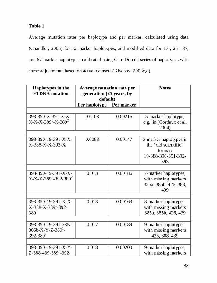
88

Table 1

Average mutation rates per haplotype and per marker, calculated using data

(Chandler, 2006) for 12-marker haplotypes, and modified data for 17-, 25-, 37,

and 67-marker haplotypes, calibrated using Clan Donald series of haplotypes with

some adjustments based on actual datasets (Klyosov, 2008c,d)

Haplotypes in the FTDNA notation

Average mutation rate per generation (25 years, by

default)

Notes

Per haplotype Per marker

393-390-X-391-X-X-X-X-X-3891-X-3892

0.0108 0.00216 5-marker haplotype, e.g., in (Cordaux et al,

2004)

393-390-19-391-X-X-X-388-X-X-392-X

0.0088 0.00147 6-marker haplotypes in the “old scientific”

format: 19-388-390-391-392-

393

393-390-19-391-X-X-X-X-X-3891-392-3892

0.013 0.00186 7-marker haplotypes, with missing markers 385a, 385b, 426, 388,

439

393-390-19-391-X-X-X-388-X-3891-392-3892

0.013 0.00163 8-marker haplotypes, with missing markers 385a, 385b, 426, 439

393-390-19-391-385a-385b-X-Y-Z-3891-392-3892

0.017 0.00189 9-marker haplotypes, with missing markers

426, 388, 439

393-390-19-391-X-Y-Z-388-439-3891-392-

0.018 0.00200 9-marker haplotypes, with missing markers

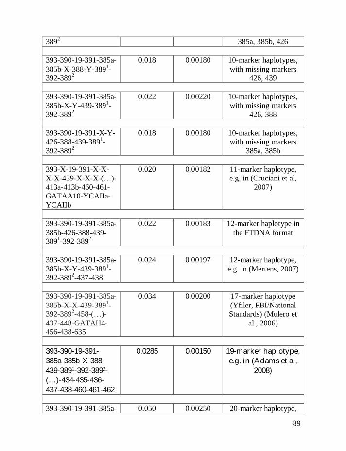
89

3892 385a, 385b, 426

393-390-19-391-385a-385b-X-388-Y-3891-392-3892

0.018 0.00180 10-marker haplotypes, with missing markers

426, 439

393-390-19-391-385a-385b-X-Y-439-3891-392-3892

0.022 0.00220 10-marker haplotypes, with missing markers

426, 388

393-390-19-391-X-Y-426-388-439-3891-392-3892

0.018 0.00180 10-marker haplotypes, with missing markers

385a, 385b 393-Х-19-391-Х-Х-Х-Х-439-Х-Х-Х-(…)- 413a-413b-460-461-GATAA10-YCAIIa-YCAIIb

0.020 0.00182 11-marker haplotype, e.g. in (Cruciani et al,

2007)

393-390-19-391-385a-385b-426-388-439-3891-392-3892

0.022 0.00183 12-marker haplotype in the FTDNA format

393-390-19-391-385a-385b-X-Y-439-3891-392-3892-437-438

0.024 0.00197 12-marker haplotype, e.g. in (Mertens, 2007)

393-390-19-391-385a-385b-X-X-439-3891-392-3892-458-(…)-437-448-GATAH4-456-438-635

0.034 0.00200 17-marker haplotype (Yfiler, FBI/National Standards) (Mulero et

al., 2006)

393-390-19-391-385a-385b-X-388-439-3891-392-3892-(…)-434-435-436-437-438-460-461-462

0.0285 0.00150 19-marker haplotype, e.g. in (Adams et al,

2008)

393-390-19-391-385a- 0.050 0.00250 20-marker haplotype,

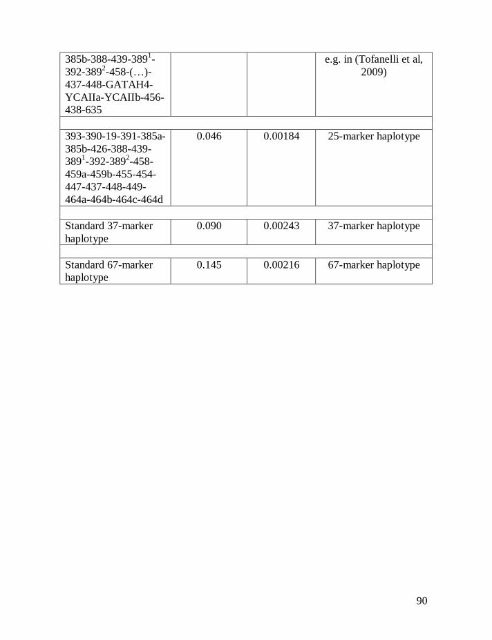
90

385b-388-439-3891-392-3892-458-(…)-437-448-GATAH4-YCAIIa-YCAIIb-456-438-635

e.g. in (Tofanelli et al, 2009)

393-390-19-391-385a-385b-426-388-439-3891-392-3892-458-459a-459b-455-454-447-437-448-449-464a-464b-464c-464d

0.046 0.00184 25-marker haplotype

Standard 37-marker haplotype

0.090 0.00243 37-marker haplotype

Standard 67-marker haplotype

0.145 0.00216 67-marker haplotype

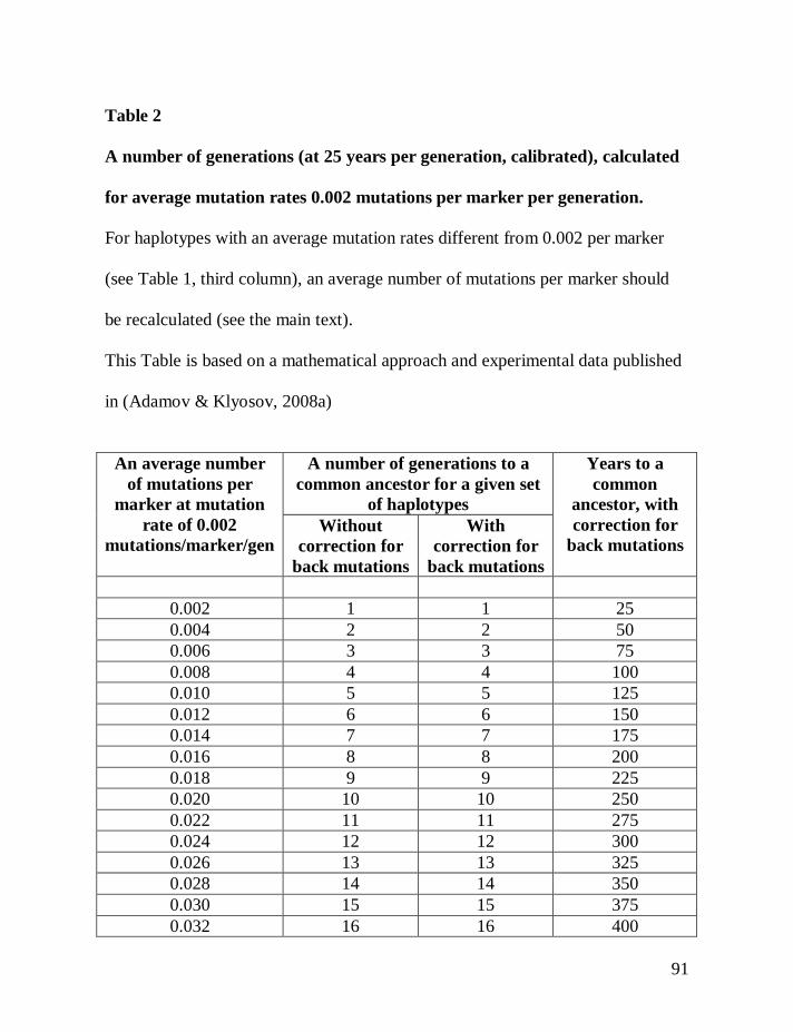
91

Table 2

A number of generations (at 25 years per generation, calibrated), calculated

for average mutation rates 0.002 mutations per marker per generation.

For haplotypes with an average mutation rates different from 0.002 per marker

(see Table 1, third column), an average number of mutations per marker should

be recalculated (see the main text).

This Table is based on a mathematical approach and experimental data published

in (Adamov & Klyosov, 2008a)

An average number

of mutations per marker at mutation

rate of 0.002 mutations/marker/gen

A number of generations to a common ancestor for a given set

of haplotypes

Years to a common

ancestor, with correction for

back mutations Without

correction for back mutations

With correction for

back mutations

0.002 1 1 25 0.004 2 2 50 0.006 3 3 75 0.008 4 4 100 0.010 5 5 125 0.012 6 6 150 0.014 7 7 175 0.016 8 8 200 0.018 9 9 225 0.020 10 10 250 0.022 11 11 275 0.024 12 12 300 0.026 13 13 325 0.028 14 14 350 0.030 15 15 375 0.032 16 16 400

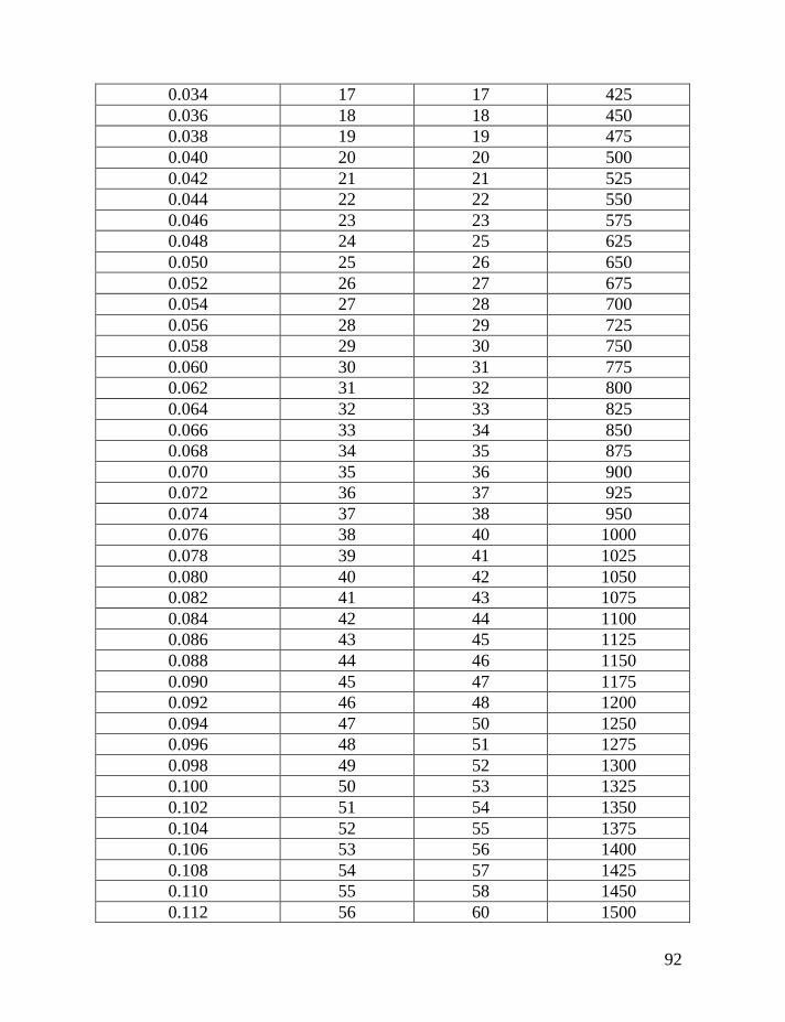
92

0.034 17 17 425 0.036 18 18 450 0.038 19 19 475 0.040 20 20 500 0.042 21 21 525 0.044 22 22 550 0.046 23 23 575 0.048 24 25 625 0.050 25 26 650 0.052 26 27 675 0.054 27 28 700 0.056 28 29 725 0.058 29 30 750 0.060 30 31 775 0.062 31 32 800 0.064 32 33 825 0.066 33 34 850 0.068 34 35 875 0.070 35 36 900 0.072 36 37 925 0.074 37 38 950 0.076 38 40 1000 0.078 39 41 1025 0.080 40 42 1050 0.082 41 43 1075 0.084 42 44 1100 0.086 43 45 1125 0.088 44 46 1150 0.090 45 47 1175 0.092 46 48 1200 0.094 47 50 1250 0.096 48 51 1275 0.098 49 52 1300 0.100 50 53 1325 0.102 51 54 1350 0.104 52 55 1375 0.106 53 56 1400 0.108 54 57 1425 0.110 55 58 1450 0.112 56 60 1500

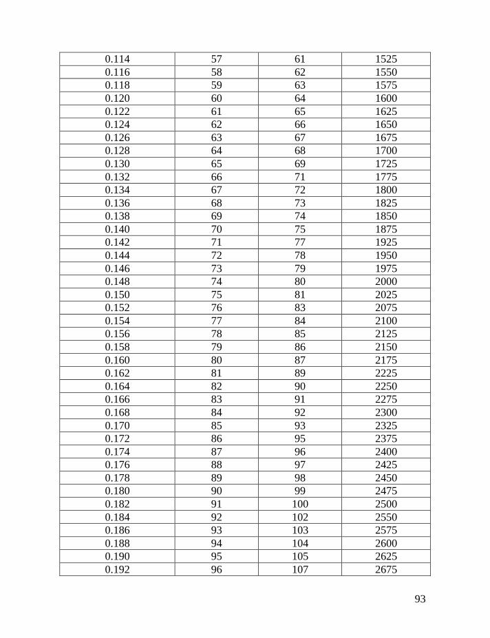
93

0.114 57 61 1525 0.116 58 62 1550 0.118 59 63 1575 0.120 60 64 1600 0.122 61 65 1625 0.124 62 66 1650 0.126 63 67 1675 0.128 64 68 1700 0.130 65 69 1725 0.132 66 71 1775 0.134 67 72 1800 0.136 68 73 1825 0.138 69 74 1850 0.140 70 75 1875 0.142 71 77 1925 0.144 72 78 1950 0.146 73 79 1975 0.148 74 80 2000 0.150 75 81 2025 0.152 76 83 2075 0.154 77 84 2100 0.156 78 85 2125 0.158 79 86 2150 0.160 80 87 2175 0.162 81 89 2225 0.164 82 90 2250 0.166 83 91 2275 0.168 84 92 2300 0.170 85 93 2325 0.172 86 95 2375 0.174 87 96 2400 0.176 88 97 2425 0.178 89 98 2450 0.180 90 99 2475 0.182 91 100 2500 0.184 92 102 2550 0.186 93 103 2575 0.188 94 104 2600 0.190 95 105 2625 0.192 96 107 2675

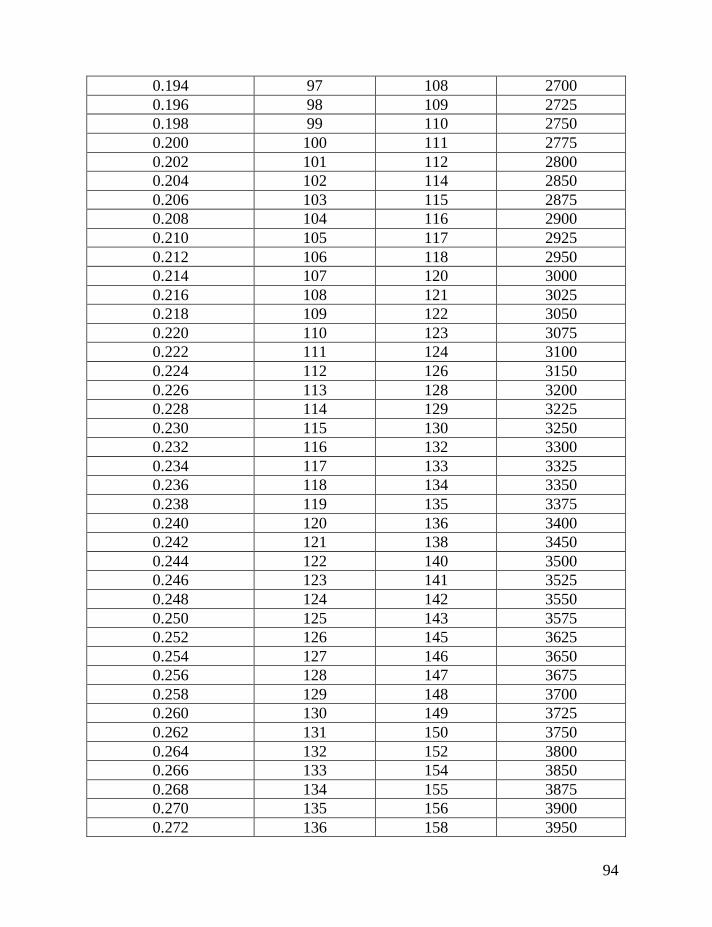
94

0.194 97 108 2700 0.196 98 109 2725 0.198 99 110 2750 0.200 100 111 2775 0.202 101 112 2800 0.204 102 114 2850 0.206 103 115 2875 0.208 104 116 2900 0.210 105 117 2925 0.212 106 118 2950 0.214 107 120 3000 0.216 108 121 3025 0.218 109 122 3050 0.220 110 123 3075 0.222 111 124 3100 0.224 112 126 3150 0.226 113 128 3200 0.228 114 129 3225 0.230 115 130 3250 0.232 116 132 3300 0.234 117 133 3325 0.236 118 134 3350 0.238 119 135 3375 0.240 120 136 3400 0.242 121 138 3450 0.244 122 140 3500 0.246 123 141 3525 0.248 124 142 3550 0.250 125 143 3575 0.252 126 145 3625 0.254 127 146 3650 0.256 128 147 3675 0.258 129 148 3700 0.260 130 149 3725 0.262 131 150 3750 0.264 132 152 3800 0.266 133 154 3850 0.268 134 155 3875 0.270 135 156 3900 0.272 136 158 3950

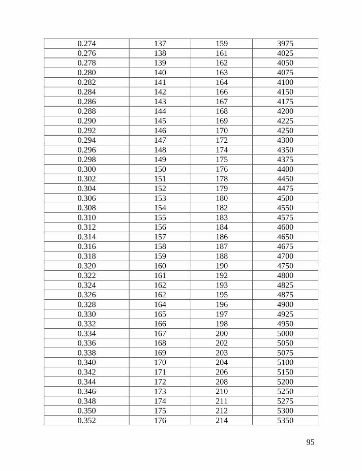
95

0.274 137 159 3975 0.276 138 161 4025 0.278 139 162 4050 0.280 140 163 4075 0.282 141 164 4100 0.284 142 166 4150 0.286 143 167 4175 0.288 144 168 4200 0.290 145 169 4225 0.292 146 170 4250 0.294 147 172 4300 0.296 148 174 4350 0.298 149 175 4375 0.300 150 176 4400 0.302 151 178 4450 0.304 152 179 4475 0.306 153 180 4500 0.308 154 182 4550 0.310 155 183 4575 0.312 156 184 4600 0.314 157 186 4650 0.316 158 187 4675 0.318 159 188 4700 0.320 160 190 4750 0.322 161 192 4800 0.324 162 193 4825 0.326 162 195 4875 0.328 164 196 4900 0.330 165 197 4925 0.332 166 198 4950 0.334 167 200 5000 0.336 168 202 5050 0.338 169 203 5075 0.340 170 204 5100 0.342 171 206 5150 0.344 172 208 5200 0.346 173 210 5250 0.348 174 211 5275 0.350 175 212 5300 0.352 176 214 5350

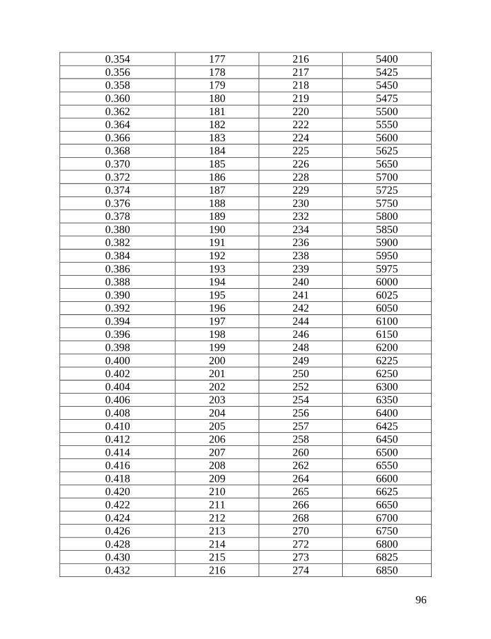
96

0.354 177 216 5400 0.356 178 217 5425 0.358 179 218 5450 0.360 180 219 5475 0.362 181 220 5500 0.364 182 222 5550 0.366 183 224 5600 0.368 184 225 5625 0.370 185 226 5650 0.372 186 228 5700 0.374 187 229 5725 0.376 188 230 5750 0.378 189 232 5800 0.380 190 234 5850 0.382 191 236 5900 0.384 192 238 5950 0.386 193 239 5975 0.388 194 240 6000 0.390 195 241 6025 0.392 196 242 6050 0.394 197 244 6100 0.396 198 246 6150 0.398 199 248 6200 0.400 200 249 6225 0.402 201 250 6250 0.404 202 252 6300 0.406 203 254 6350 0.408 204 256 6400 0.410 205 257 6425 0.412 206 258 6450 0.414 207 260 6500 0.416 208 262 6550 0.418 209 264 6600 0.420 210 265 6625 0.422 211 266 6650 0.424 212 268 6700 0.426 213 270 6750 0.428 214 272 6800 0.430 215 273 6825 0.432 216 274 6850

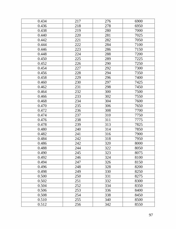
97

0.434 217 276 6900 0.436 218 278 6950 0.438 219 280 7000 0.440 220 281 7025 0.442 221 282 7050 0.444 222 284 7100 0.446 223 286 7150 0.448 224 288 7200 0.450 225 289 7225 0.452 226 290 7250 0.454 227 292 7300 0.456 228 294 7350 0.458 229 296 7400 0.460 230 297 7425 0.462 231 298 7450 0.464 232 300 7500 0.466 233 302 7550 0.468 234 304 7600 0.470 235 306 7650 0.472 236 308 7700 0.474 237 310 7750 0.476 238 311 7775 0.478 239 313 7825 0.480 240 314 7850 0.482 241 316 7900 0.484 242 318 7950 0.486 242 320 8000 0.488 244 322 8050 0.490 245 323 8075 0.492 246 324 8100 0.494 247 326 8150 0.496 248 328 8200 0.498 249 330 8250 0.500 250 331 8275 0.502 251 332 8300 0.504 252 334 8350 0.506 253 336 8400 0.508 254 338 8450 0.510 255 340 8500 0.512 256 342 8550

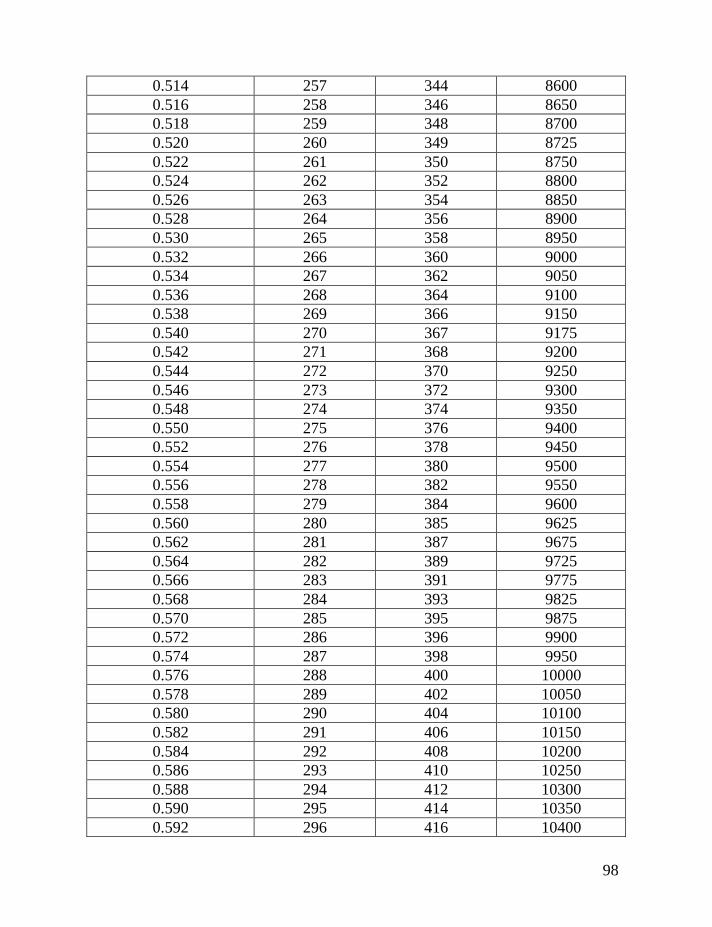
98

0.514 257 344 8600 0.516 258 346 8650 0.518 259 348 8700 0.520 260 349 8725 0.522 261 350 8750 0.524 262 352 8800 0.526 263 354 8850 0.528 264 356 8900 0.530 265 358 8950 0.532 266 360 9000 0.534 267 362 9050 0.536 268 364 9100 0.538 269 366 9150 0.540 270 367 9175 0.542 271 368 9200 0.544 272 370 9250 0.546 273 372 9300 0.548 274 374 9350 0.550 275 376 9400 0.552 276 378 9450 0.554 277 380 9500 0.556 278 382 9550 0.558 279 384 9600 0.560 280 385 9625 0.562 281 387 9675 0.564 282 389 9725 0.566 283 391 9775 0.568 284 393 9825 0.570 285 395 9875 0.572 286 396 9900 0.574 287 398 9950 0.576 288 400 10000 0.578 289 402 10050 0.580 290 404 10100 0.582 291 406 10150 0.584 292 408 10200 0.586 293 410 10250 0.588 294 412 10300 0.590 295 414 10350 0.592 296 416 10400

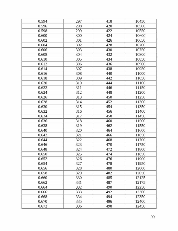
99

0.594 297 418 10450 0.596 298 420 10500 0.598 299 422 10550 0.600 300 424 10600 0.602 301 426 10650 0.604 302 428 10700 0.606 303 430 10750 0.608 304 432 10800 0.610 305 434 10850 0.612 306 436 10900 0.614 307 438 10950 0.616 308 440 11000 0.618 309 442 11050 0.620 310 444 11100 0.622 311 446 11150 0.624 312 448 11200 0.626 313 450 11250 0.628 314 452 11300 0.630 315 454 11350 0.632 316 456 11400 0.634 317 458 11450 0.636 318 460 11500 0.638 319 462 11550 0.640 320 464 11600 0.642 321 466 11650 0.644 322 468 11700 0.646 323 470 11750 0.648 324 472 11800 0.650 325 474 11850 0.652 326 476 11900 0.654 327 478 11950 0.656 328 480 12000 0.658 329 482 12050 0.660 330 485 12125 0.662 331 487 12175 0.664 332 490 12250 0.666 333 492 12300 0.668 334 494 12350 0.670 335 496 12400 0.672 336 498 12450

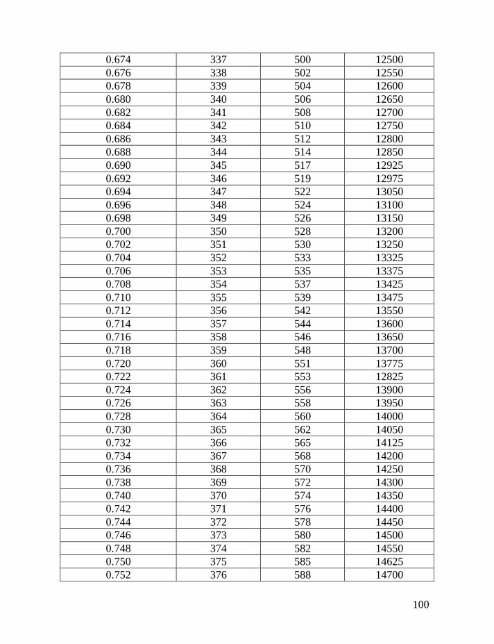
100

0.674 337 500 12500 0.676 338 502 12550 0.678 339 504 12600 0.680 340 506 12650 0.682 341 508 12700 0.684 342 510 12750 0.686 343 512 12800 0.688 344 514 12850 0.690 345 517 12925 0.692 346 519 12975 0.694 347 522 13050 0.696 348 524 13100 0.698 349 526 13150 0.700 350 528 13200 0.702 351 530 13250 0.704 352 533 13325 0.706 353 535 13375 0.708 354 537 13425 0.710 355 539 13475 0.712 356 542 13550 0.714 357 544 13600 0.716 358 546 13650 0.718 359 548 13700 0.720 360 551 13775 0.722 361 553 12825 0.724 362 556 13900 0.726 363 558 13950 0.728 364 560 14000 0.730 365 562 14050 0.732 366 565 14125 0.734 367 568 14200 0.736 368 570 14250 0.738 369 572 14300 0.740 370 574 14350 0.742 371 576 14400 0.744 372 578 14450 0.746 373 580 14500 0.748 374 582 14550 0.750 375 585 14625 0.752 376 588 14700

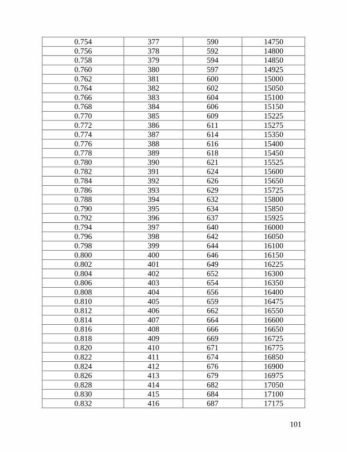
101

0.754 377 590 14750 0.756 378 592 14800 0.758 379 594 14850 0.760 380 597 14925 0.762 381 600 15000 0.764 382 602 15050 0.766 383 604 15100 0.768 384 606 15150 0.770 385 609 15225 0.772 386 611 15275 0.774 387 614 15350 0.776 388 616 15400 0.778 389 618 15450 0.780 390 621 15525 0.782 391 624 15600 0.784 392 626 15650 0.786 393 629 15725 0.788 394 632 15800 0.790 395 634 15850 0.792 396 637 15925 0.794 397 640 16000 0.796 398 642 16050 0.798 399 644 16100 0.800 400 646 16150 0.802 401 649 16225 0.804 402 652 16300 0.806 403 654 16350 0.808 404 656 16400 0.810 405 659 16475 0.812 406 662 16550 0.814 407 664 16600 0.816 408 666 16650 0.818 409 669 16725 0.820 410 671 16775 0.822 411 674 16850 0.824 412 676 16900 0.826 413 679 16975 0.828 414 682 17050 0.830 415 684 17100 0.832 416 687 17175

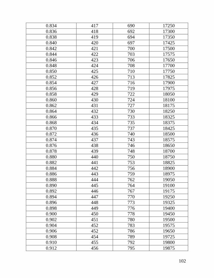
102

0.834 417 690 17250 0.836 418 692 17300 0.838 419 694 17350 0.840 420 697 17425 0.842 421 700 17500 0.844 422 703 17575 0.846 423 706 17650 0.848 424 708 17700 0.850 425 710 17750 0.852 426 713 17825 0.854 427 716 17900 0.856 428 719 17975 0.858 429 722 18050 0.860 430 724 18100 0.862 431 727 18175 0.864 432 730 18250 0.866 433 733 18325 0.868 434 735 18375 0.870 435 737 18425 0.872 436 740 18500 0.874 437 743 18575 0.876 438 746 18650 0.878 439 748 18700 0.880 440 750 18750 0.882 441 753 18825 0.884 442 756 18900 0.886 443 759 18975 0.888 444 762 19050 0.890 445 764 19100 0.892 446 767 19175 0.894 447 770 19250 0.896 448 773 19325 0.898 449 776 19400 0.900 450 778 19450 0.902 451 780 19500 0.904 452 783 19575 0.906 452 786 19650 0.908 454 789 19725 0.910 455 792 19800 0.912 456 795 19875

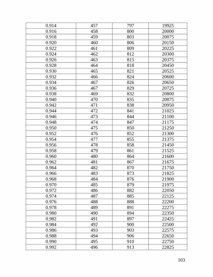
103

0.914 457 797 19925 0.916 458 800 20000 0.918 459 803 20075 0.920 460 806 20150 0.922 461 809 20225 0.924 462 812 20300 0.926 463 815 20375 0.928 464 818 20450 0.930 465 821 20525 0.932 466 824 20600 0.934 467 826 20650 0.936 467 829 20725 0.938 469 832 20800 0.940 470 835 20875 0.942 471 838 20950 0.944 472 841 21025 0.946 473 844 21100 0.948 474 847 21175 0.950 475 850 21250 0.952 476 852 21300 0.954 477 855 21375 0.956 478 858 21450 0.958 479 861 21525 0.960 480 864 21600 0.962 481 867 21675 0.964 482 870 21750 0.966 483 873 21825 0.968 484 876 21900 0.970 485 879 21975 0.972 486 882 22050 0.974 487 885 22125 0.976 488 888 22200 0.978 489 891 22275 0.980 490 894 22350 0.982 491 897 22425 0.984 492 900 22500 0.986 493 903 22575 0.988 494 906 22650 0.990 495 910 22750 0.992 496 913 22825

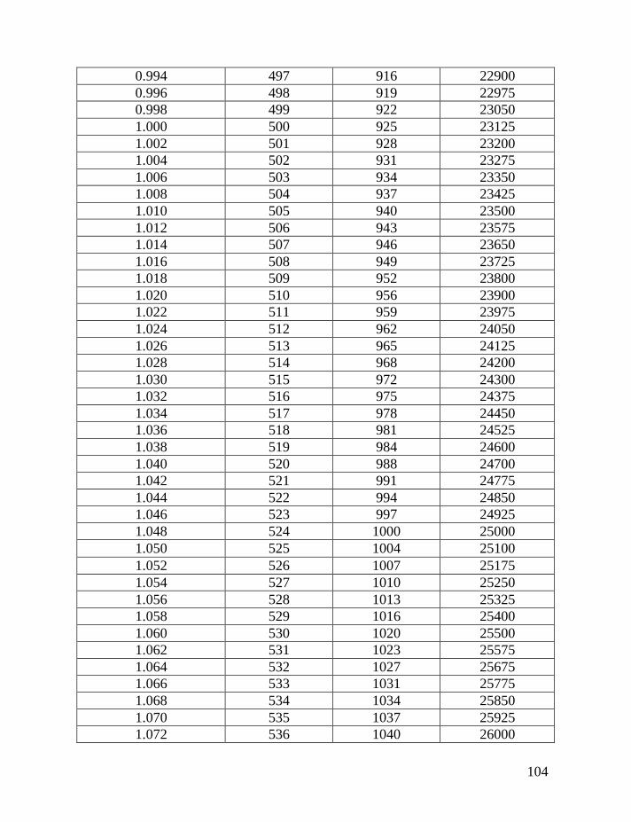
104

0.994 497 916 22900 0.996 498 919 22975 0.998 499 922 23050 1.000 500 925 23125 1.002 501 928 23200 1.004 502 931 23275 1.006 503 934 23350 1.008 504 937 23425 1.010 505 940 23500 1.012 506 943 23575 1.014 507 946 23650 1.016 508 949 23725 1.018 509 952 23800 1.020 510 956 23900 1.022 511 959 23975 1.024 512 962 24050 1.026 513 965 24125 1.028 514 968 24200 1.030 515 972 24300 1.032 516 975 24375 1.034 517 978 24450 1.036 518 981 24525 1.038 519 984 24600 1.040 520 988 24700 1.042 521 991 24775 1.044 522 994 24850 1.046 523 997 24925 1.048 524 1000 25000 1.050 525 1004 25100 1.052 526 1007 25175 1.054 527 1010 25250 1.056 528 1013 25325 1.058 529 1016 25400 1.060 530 1020 25500 1.062 531 1023 25575 1.064 532 1027 25675 1.066 533 1031 25775 1.068 534 1034 25850 1.070 535 1037 25925 1.072 536 1040 26000

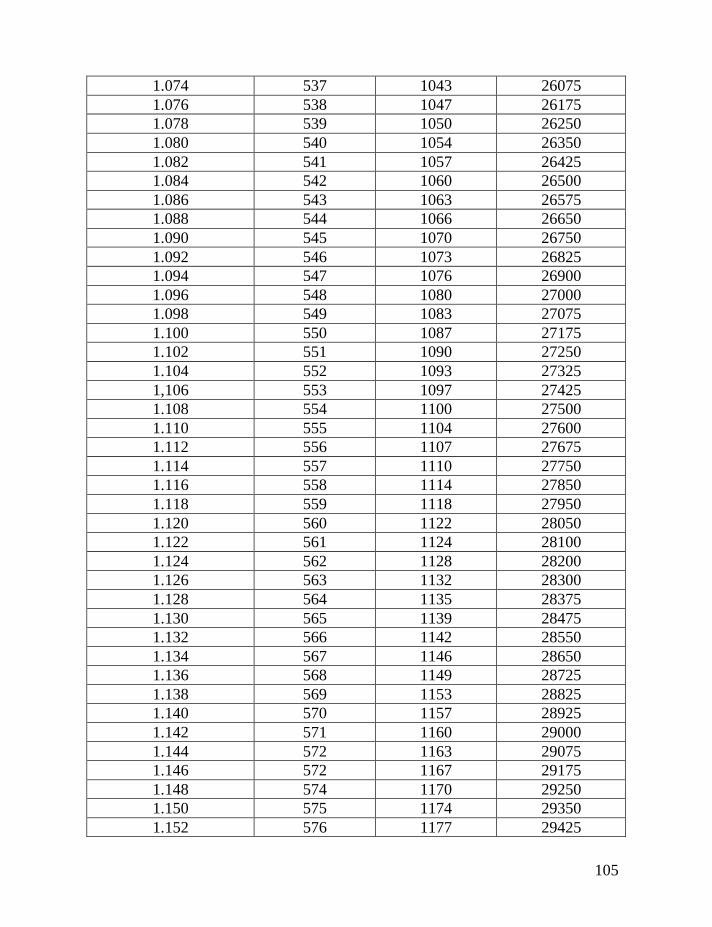
105

1.074 537 1043 26075 1.076 538 1047 26175 1.078 539 1050 26250 1.080 540 1054 26350 1.082 541 1057 26425 1.084 542 1060 26500 1.086 543 1063 26575 1.088 544 1066 26650 1.090 545 1070 26750 1.092 546 1073 26825 1.094 547 1076 26900 1.096 548 1080 27000 1.098 549 1083 27075 1.100 550 1087 27175 1.102 551 1090 27250 1.104 552 1093 27325 1,106 553 1097 27425 1.108 554 1100 27500 1.110 555 1104 27600 1.112 556 1107 27675 1.114 557 1110 27750 1.116 558 1114 27850 1.118 559 1118 27950 1.120 560 1122 28050 1.122 561 1124 28100 1.124 562 1128 28200 1.126 563 1132 28300 1.128 564 1135 28375 1.130 565 1139 28475 1.132 566 1142 28550 1.134 567 1146 28650 1.136 568 1149 28725 1.138 569 1153 28825 1.140 570 1157 28925 1.142 571 1160 29000 1.144 572 1163 29075 1.146 572 1167 29175 1.148 574 1170 29250 1.150 575 1174 29350 1.152 576 1177 29425

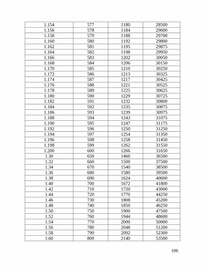
106

1.154 577 1180 28500 1.156 578 1184 29600 1.158 579 1188 29700 1.160 580 1192 29800 1.162 581 1195 29875 1.164 582 1198 29950 1.166 583 1202 30050 1.168 584 1206 30150 1.170 585 1210 30250 1.172 586 1213 30325 1.174 587 1217 30425 1.176 588 1221 30525 1.178 589 1225 30625 1.180 590 1229 30725 1.182 591 1232 30800 1.184 592 1235 30875 1.186 593 1239 30975 1.188 594 1243 31075 1.190 595 1247 31175 1.192 596 1250 31250 1.194 597 1254 31350 1.196 598 1258 31450 1.198 599 1262 31550 1.200 600 1266 31650 1.30 650 1460 36500 1.32 660 1500 37500 1.34 670 1540 38500 1.36 680 1580 39500 1.38 690 1624 40600 1.40 700 1672 41800 1.42 710 1720 43000 1.44 720 1770 44250 1.46 730 1808 45200 1.48 740 1850 46250 1.50 750 1900 47500 1.52 760 1944 48600 1.54 770 2000 50000 1.56 780 2048 51200 1.58 790 2092 52300 1.60 800 2140 53500

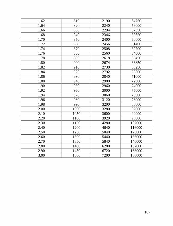
107

1.62 810 2190 54750 1.64 820 2240 56000 1.66 830 2294 57350 1.68 840 2346 58650 1.70 850 2400 60000 1.72 860 2456 61400 1.74 870 2508 62700 1.76 880 2560 64000 1.78 890 2618 65450 1.80 900 2674 66850 1.82 910 2730 68250 1.84 920 2792 69800 1.86 930 2840 71000 1.88 940 2900 72500 1.90 950 2960 74000 1.92 960 3000 75000 1.94 970 3060 76500 1.96 980 3120 78000 1.98 990 3200 80000 2.00 1000 3280 82000 2.10 1050 3600 90000 2.20 1100 3920 98000 2.30 1150 4280 107000 2.40 1200 4640 116000 2.50 1250 5040 126000 2.60 1300 5440 136000 2.70 1350 5840 146000 2.80 1400 6280 157000 2.90 1450 6720 168000 3.00 1500 7200 180000

108

Legends to Figures

Figure 1. The 84-haplotype 25-marker tree for R1a1 Donald haplotypes. The

tree was composed according to data of the DNA Project Clan Donald (2008).

The tree shows 21 identical “base” haplotypes sitting on top of the tree.

Figure 2. The 25-marker haplotype tree for Basque R1b1 (mainly R1b1b2)

haplotypes. The 17-haplotype tree was composed according to data of the

Basque DNA Project (2008).

Figure 3. The 19-marker haplotype tree for Iberian R1b1 haplotypes. The

tree was composed according to data published (Adams et al, 2008).

Figure 4. The 12-marker haplotype tree for J1 haplotypes with mutated

DYS426. The tree was composed from haplotypes collected in YSearch data

base. Bearers of haplotypes 002, 003, 004, 005, 006, 008, 010 and 011 have

Jewish surnames.

Figure 5. The 20-marker haplotype tree for J1-M267 haplotypes. The tree

contains 282 haplotypes, and was composed according to data published

(Tofanelli et al, 2009).

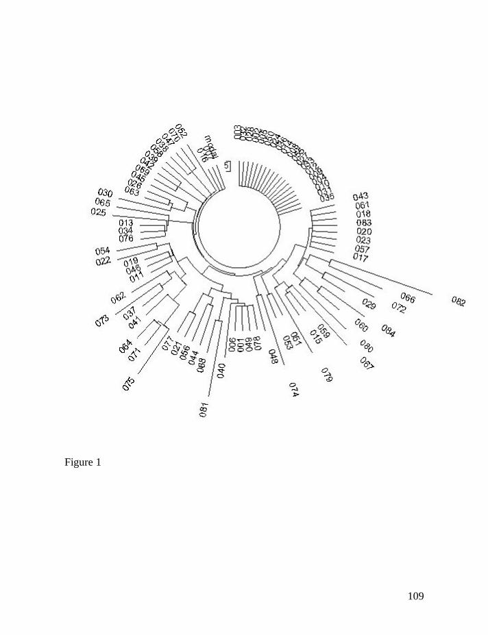
109

Figure 1

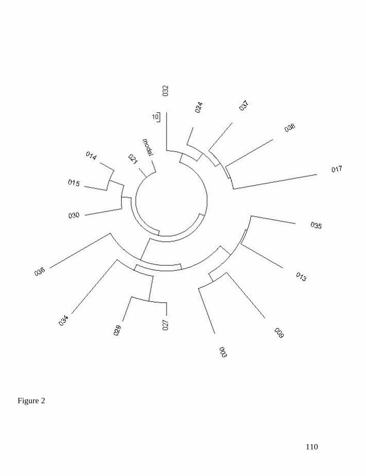
110

Figure 2

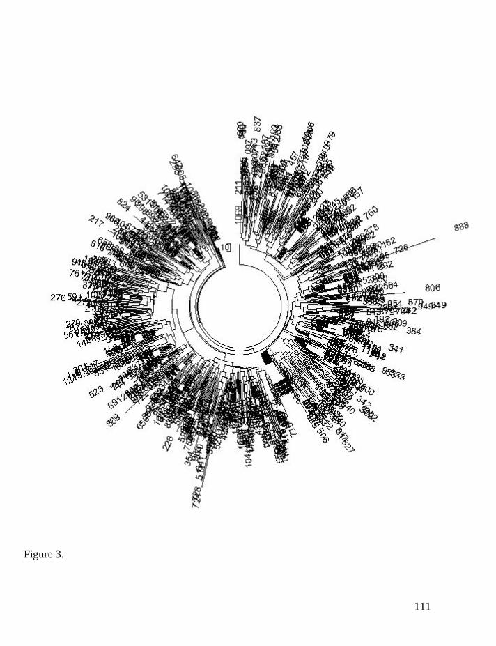
111

Figure 3.

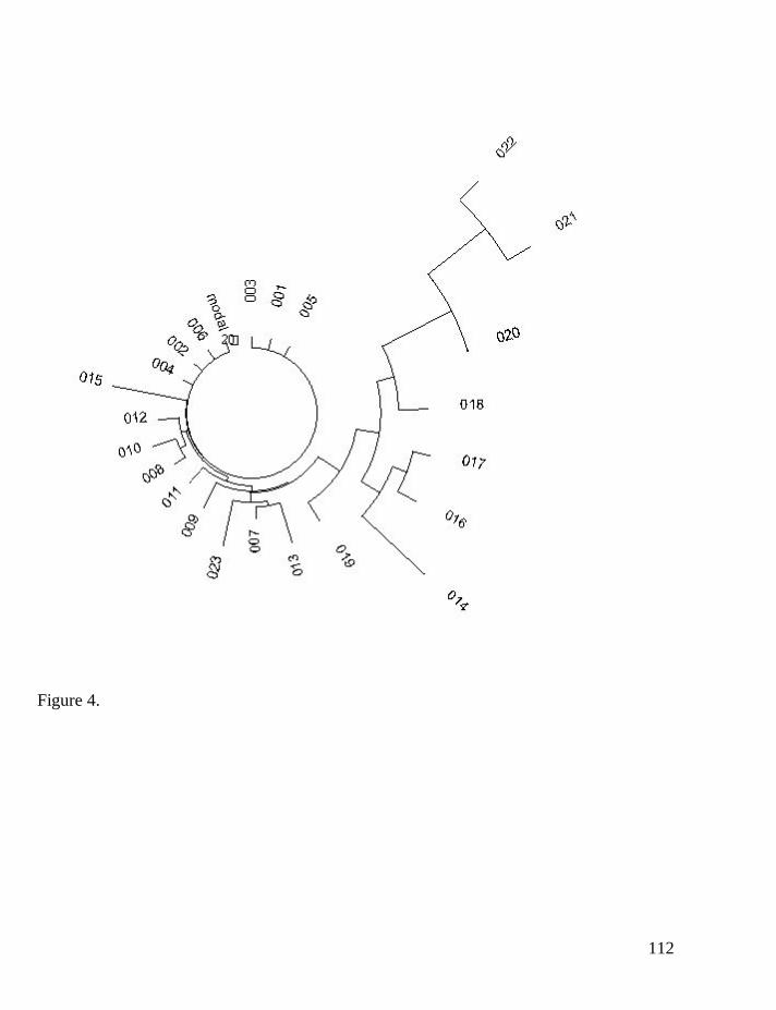
112

Figure 4.

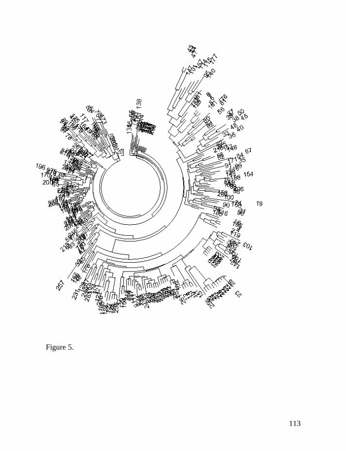
113

Figure 5.