Do Cash Transfers Promoting Early Childhood

Development Have Unintended Consequences on Fertility?¤

Pedro Carneiro Lucy Kraftman Imran Rasul Molly Scotty

September 2021

Abstract

There has been a stark rise in direct cash transfer programs to the poor, and in policy

interest in interventions targeting outcomes in early childhood. We draw these trends together

to study whether interventions o¤ering cash transfers to pregnant mothers to promote early

childhood development, unintentionally induce those not pregnant to bring forward birth

timing in order to become eligible for the receipt of such transfers. We do so in the context of

rural Northern Nigeria, where the majority of households reside in extreme poverty, are credit

constrained and food insecure, and frequently experience aggregate shocks. Contraceptives

are unavailable and men largely drive fertility choices, yet the costs of bringing forward birth

timing mostly operate through worse maternal and child health. We present evidence from

a randomized control trial evaluating an intervention o¤ering high-valued and long-lasting

unconditional cash transfers to pregnant mothers. We examine how this impacted fertility

dynamics among 1700 households in which women were not pregnant at baseline, tracked over

four years from the intervention initiation. We document precise null impacts on the timing of

births, total births and composition of households becoming pregnant over our study period.

The reason is a combination of three factors: (i) women retain full control over the use of

additional resources they bring into their household; (ii) women have available productive

investment opportunities in their own businesses; (iii) they choose to transfer few resources to

husbands. Hence ultimately men have weak private incentives to alter birth timing. Based

on this constellation of factors, we use DHS surveys to classify low-income countries into

those that are more or less likely to see fertility consequences when cash transfers for early

childhood development are targeted to pregnant mothers. JEL Classi…cation I15, O15.

¤We gratefully acknowledge …nancial support from DfID, the ESRC CPP at IFS (ES/H021221/1), the ESRC forCEMMAP (ES/P008909/1) and the ERC (ERC-2015-CoG-682349). We thank Save the Children International andAction Against Hunger International, and the OPM Abuja Survey team led by Femi Adegoke. Oriana Bandiera,John List, David Phillips, Rodrigo Soares, Michela Tincani and numerous seminar participants provided valuablecomments. Human subjects approval was obtained from the National Health Research Ethics Committee of Nigeria(NHREC/01/01/2007-30/06/2014c). The study is registered (AEARCTR-0000454). All errors remain our own.

yCarneiro: UCL, IFS, CEMMAP, FAIR-NHH, p.carneiro@ucl.ac.uk; Kraftman: IFS, lucy.kraftman@ifs.org.uk;Rasul: UCL and IFS, i.rasul@ucl.ac.uk; Scott: National Centre for Social Research, molly.scott@natcen.ac.uk.

1

1 Introduction

One of the most prominent changes in the landscape of development policy has been the increased

use of direct cash transfers to the poor. 119 low-income countries have now implemented some

unconditional cash transfer program, and a further 52 have established conditional cash transfer

programs [Handa et al. 2017]. This trend extends to Sub Saharan Africa, where 40 countries had

implemented unconditional cash transfer programs by 2014, double the number in 2010 [De Groot

et al. 2017]. Cash transfers to the poor are likely to become further entrenched as such policies

have been a leading response to the COVID-19 crisis in the developing world. An established

body of evidence shows cash transfers are an e¤ective means by which to reduce poverty and

increase household welfare through multiple channels including those related to education, health

and nutrition, savings and investment [Bastagli et al. 2018].

Equally impressive has been the rise in policy maker interest in promoting human capital

development in early life. There has been growing recognition that 250 million children in low-

and middle-income countries are at risk of not meeting their developmental potential because of

inadequate nutrition and stimulation in early life [Black et al. 2017], and such deprivation in

early life has consequences throughout the life cycle [Almond and Currie 2011]. Evaluations from

across settings – including in Sub Saharan Africa – show interventions to promote human capital

development in early life can generate large private, social and intergenerational returns.1

These powerful trends are now intertwining, with the provision of cash transfers increasingly

being used to promote early childhood development. Common features of such interventions are

that resources are provided directly to mothers, and that eligibility hinges on whether a woman

within the household is identi…ed to be pregnant, or to have a very young child. We study whether

and how the availability of such programs impact households without pregnant women in them

and so not initially eligible for the cash transfers. More precisely, in a context of extreme economic

destitution, we study whether the o¤er of cash transfers promoting early childhood development

induces endogenous fertility responses among not pregnant households, in order to gain access to

the resources on o¤er and ease some of the economic hardships they would otherwise face.

We do so by presenting evidence from a randomized control trial evaluation of program pro-

viding extremely high-valued cash transfers to promote early child development, in a context of

extreme poverty (two states in Northern Nigeria). The program is known as the Child Devel-

opment Grant Program (CDGP). It provides any household in which a women is veri…ed to be

pregnant (via a urine test) a bundle of: (i) information to mothers and fathers on recommended

practices related to pregnancy and infant feeding; (ii) unconditional cash transfers, paid directly

to mothers conditional on their pregnancy being veri…ed, so while the child is in utero, each month

1Impacts of interventions in early life have been found on cognitive development and health [Campbell et al.2014, Conti et al. 2016, Attanasio et al. 2019, Doyle 2019, Carneiro et al. 2021, Field and Ma¢oli 2021, Justinoet al. 2021], schooling and labor market productivity [Hoddinott et al. 2008, Gertler et al. 2014] and acrossgenerations [Heckman and Karapakula 2019].

2

until the child turns 24-months old. Targeting children in utero re‡ects the belief that providing

resources to households in the critical window of the …rst 1000 days of life generate higher returns

on child outcomes than those targeting children later in life. Transfers are provided for one child,

not later borns, although there is no requirement for the pregnancy to occur closer to baseline.

Enrolment into the program was announced to be in open for four years from baseline, providing

a narrow window for non pregnant households to endogenously accelerate birth timing within.

The value of the unconditional cash transfer is US$22 per month. However benchmarked, this

is a substantial amount, corresponding to 85% of women’s baseline monthly earnings or 26% of

monthly food expenditures. The cumulative resource ‡ow available to eligible households amounts

to over $500, akin to a big push on the same scale as asset transfer policies [Banerjee et al. 2015,

Bandiera et al. 2017]. Moreover, the fact that women know transfers will be provided monthly

over this period of the child’s life provides them with a more stable ‡ow of resources than is

available from labor activities: the transfers almost act as a de facto temporary basic income for

pregnant mothers.

Understanding fertility responses among those not immediately eligible is important because

in low-income contexts even small changes in birth timing and total fertility can have large and

persistent impacts on the welfare of children and mothers, through well-documented risks to

maternal and child health [DaVanzo et al. 2004, WHO 2005, Pimentel et al. 2020, Damtie et al.

2021].2 Our study context – Jigawa and Zamfara states in Northern Nigeria – is an area of intense

economic destitution and any unintended consequence on fertility might by especially costly. As

Figure A1 shows, this region is yet to experience the demographic transition, with total fertility

rates close to six and so well above the average in Sub Saharan Africa (Panel A); birth spacing is

30 months (Panel B) with around 30% of births being spaced less than 24 months apart (Panel C),

a threshold marker for detrimental impacts for mothers and children [WHO 2005]; contraceptive

usage is very limited, with fewer than 10% of married women in Jigawa and Zamfara states in

Northern Nigeria reporting using any form of contraception (Panel D).

These features are re‡ected in our evaluation sample, that is purposefully collected in order to

answer our core research question. Our sample comprises households not immediately eligible for

the program because the main women in them is not pregnant when the program is initiated. At

baseline, 85% of our sample households live in extreme poverty – so below the $190/day threshold.

Infant mortality rates are 90 per 1000 children, and the vast majority of women entirely lack access

to contraceptives. Both factors result in high fertility rates – at baseline, women in our sample

2The WHO recommends a minimum birth interval of 33 months or more to ensure the maximum health bene…tsfor mothers and newborns [WHO 2005]. Spacing the child for a minimum of two years reduces infant mortality by50% [DaVanzo et al. 2004]. Short birth spacing has been linked with di¤erent adverse pregnancy and childbirthoutcomes such as low birth weight, preterm birth, congenital anomalies autism, small size for gestational age, andneonatal, infant and child mortality. Moreover, women with short birth spacing are at high risk of developing hyper-tensive disorders of pregnancy, anemia, third-trimester bleeding, premature rupture of membranes, and puerperalendometritis [Damtie et al. 2021].

3

are aged 24 and have 4 children on average, yet are far from completing their fertility cycle. In

this region the agricultural cycle includes a lean season in which households face food shortages,

and have to resort to extreme coping strategies. Households have access to highly imperfect credit

markets that limit household’s ability to smooth consumption, and our sample villages are subject

to frequent aggregate shocks. Finally state capacity is limited, so even though the intervention we

study is delivered by NGOs and announced to have a …xed window of enrolment, its introduction

might not signify permanent changes in the social assistance on o¤er.

All these features of the environment create economic forces pushing in the same direction, to

provide households high-powered incentives to accelerate the timing of births in order to become

eligible for cash transfers, or to have an additional child if their fertility cycle was already complete.

The marginal bene…t of doing so is that such resources might then be used to ameliorate

economic pressures, as well as being used to invest in the human capital of young children. The

marginal cost of doing so is that by reducing birth spacing, there are risks to maternal and child

health. These marginal bene…ts and marginal costs are spread slightly di¤er across household

members: husbands, wives and children.

Furthermore, we note that Nigeria is a patriarchal society where bride prices are still common,

with wives often perceived as being purchased by their husbands. This leads to decisions about

reproduction residing primarily in the hands of the husband and his family. These features of

our study context are well documented by work in demography and gender studies [Caldwell and

Caldwell 1987, 1988, Odimegwu and Adenini 2014, 2015]. If men are less informed about the

maternal risks of shifting birth timing or total fertility than their wives [Ashraf et al. 2020a],

yet have some say over fertility, the imbalance between spouses in terms of who drives fertility

decisions and who bears the marginal costs of shifting birth timing can further tilt the balance

towards households bringing forward the timing of births in order to gain access to these resources.

Our research design and data collection allow us to present evidence to causally link multiple

margins of fertility-related responses to the o¤er of cash transfers conditional on pregnancy, and

link them to these marginal bene…ts and marginal costs across household members.

Our evaluation covers households in 210 villages: two thirds of them are randomly assigned

to treatment, where the intervention is rolled out from baseline. In earlier work, Carneiro et

al. [2021], we evaluated the intervention tracking 3700 women already veri…ed to be pregnant

at baseline. Among that sample, by construction, there is no endogenous fertility response to

the intervention. For the children that were in utero at baseline, we …nd persistent and large

positive impacts on child anthropometrics, such as their height-for-age Z-scores, and statistically

and economically signi…cant reductions in the incidence of child illness, improvements in child

nutrition, deworming and vaccination rates. We estimate an IRR to the program, in terms of

child outcomes, of at least 10% under plausible assumptions. Hence the program is cost e¤ective

among the cross section of women that happen to be pregnant at baseline. In this paper we shed

light on whether this extends to the far larger cohort of women not pregnant at baseline.

4

Relative to Carneiro et al. [2021] we focus on an entirely separate sample of 1700 women that

were not pregnant at baseline. We shed light on endogenous fertility responses to the intervention

o¤er of cash transfers by tracking this sample of women not pregnant at baseline at two- and

four-years post intervention.

Our four year study timeline is thus long enough to consider behavioral responses among

households: (i) that decide to shift forward their birth timing in order to start receiving transfers

earlier than they otherwise would have if they maintained the fertility path they had planned pre-

intervention; (ii) towards the end of the study period and lifetime of enrolment into the program,

who otherwise risk losing access to the high-valued cash transfers altogether. On (i), households

demand for short term liquidity has been experimentally documented in other low-income contexts,

including in response to lean seasons and ‡uctuating income streams from agriculture [Casaburi

and Willis 2018, Casaburi and Macchiavello 2019, Fink et al. 2020, Mobarak et al. 2021]. We

bring this issue to study of cash transfers targeting pregnant mothers, whereby households can

gain liquidity to ease economic hardships and uncertainty, but only conditional on women in them

becoming pregnant. On (ii) we note that in other studies where large big push resource injections

are o¤ered to households, take-up rates are close to 100%. We extend this to a context in which

cumulative resources of around $500 gain be gained by households if they shift birth timing into

the four-year window of open enrolment into the program.

Results First, we document precise null impacts on the fertility dynamics of women not pregnant

at baseline over the study period. This is both in terms of overall fertility (a quantum e¤ect) and

the exact timing of births as identi…ed from survival analysis (a tempo e¤ect). On the number of

children born, these null e¤ects are precise, the 95% con…dence interval on our treatment e¤ect

rules out a magnitude larger than 094 between baseline and the two-year midline, and larger

than 066 between midline and the four-year endline. We also …nd very limited impacts on the

composition of households that become pregnant during our four-year study period.

Second, for women not pregnant at baseline, but who gave birth during our study period, the

intervention still leads to improvements in child outcomes. For example, at midline: (i) children’s

height-for-age Z-scores (HAZ) improve by 26 ; (ii) there is a reduced incidence of stunting of

107pp, corresponding to an 22% reduction. Stunting is the best measure of cumulative e¤ects of

chronic nutritional deprivation, and is therefore a key indicator of long-term well-being. On health,

an index of health outcomes improves by 16 at midline, and this improvement is sustained at

endline, where the index rises by 25 over controls.

Overall, we show the trajectory of child development is very similar between the children of

mothers that were not pregnant at baseline and only become eligible through pregnancy, and those

that were pregnant at baseline and so automatically eligible at baseline, as we previously analyzed

in Carneiro et al. [2021]. We also show there are no detrimental impacts on maternal health

from the o¤er of cash transfers. These results reinforce the …nding that any endogenous fertility

5

responses to the o¤er of cash transfers by households not immediately eligible for the intervention

is second order.

Our third set of results explain what causes the null e¤ects on fertility dynamics, despite

strong economic incentives households face in this setting to become eligible for the cash transfers

by bringing forward the timing of births, or to alter the quantity of births for those families who

were close to the end of their planned fertility. To do so, we reiterate the wedge between wives

– who primarily bear the marginal costs of shifts in birth timing or total fertility – and their

husbands, who largely drive fertility decisions given the absence of contraceptives. We thus dig

deeper to examine the role of husbands.

We show the null fertility impacts can be explained through a combination of three factors:

(i) there is separate spheres decision making in these households [Lundberg and Pollak 1993,

Browning et al. 2010], so women entirely retain control of any resources they bring into the

household (such as earnings), including how additional resources such as cash transfers from the

intervention are spent; (ii) women have high labor force participation rates and have productive

investment opportunities available to them through their own businesses; (iii) few resources leak

to husbands for their private gain, except via household public goods of higher food consumption

and savings in the longer run.

These factors combine to imply husbands have weak private incentive to change fertility dynam-

ics in response to the program, all else equal, despite the strong decision making rights husbands

have over fertility in this context.

We underpin this interpretation of our null results using within-sample variation in fertility

responses between women that were not pregnant at baseline and: (i) report having full autonomy

over how to spend any exogenous increase in resources they bring into the household; (ii) are self-

employed; (iii) have opportunities for business investment (either because they own productive

livestock or have other business assets at baseline), versus women for whom none of these three

conditions are satis…ed at baseline. We view the husbands of the former group of women as having

relatively weaker incentives to bring forward birth timing, and the latter as having husbands with

relatively stronger incentives to do so – either because they can appropriate the cash, or their wife

willingly transfers resources to them because she lacks investment opportunities of her own.

We continue to …nd null fertility impacts among the former group of households. In contrast,

we …nd that for the latter group, households are 92pp signi…cantly more likely to have any children

born between baseline and midline (corresponding to a 16% increase over comparable households

in controls). As is intuitive, this increase in fertility for husbands with stronger incentives occurs

within the …rst two years of open enrolment into the program. Testing for di¤erences across

households where husbands have weaker and stronger incentives, the di¤erential impact on the

number of children born between baseline and midline is statistically di¤erent ( = 091).

We rule out further alternative explanations for the null impacts on the timing of fertility

unrelated to any speci…c role of husbands. For example, we consider alternatives related to birth

6

spacing and the demand for additional children. We show that birth spacing – while low – is not

close to its biological lower bound [WHO 2005]. It is feasible for the vast majority of households

to bring forward birth timing if they choose to. We also show the results are not driven by women

close to the end of their fertility cycle and so perhaps with little desire for additional children. We

do so by documenting null impacts for households at di¤erent stages of the fertility cycle.

We also rule out that households expect the o¤er of cash transfers from the intervention to be

available for the foreseeable future. Given transfers are only available for one child, and fertility

rates are high to begin with, households might be secure in the knowledge that they will eventually

receive the transfers without having to adjust their planned fertility path. At its initiation, the

program is announced to be in place for four years. This is reinforced by a further announcement

– close to our four-year endline – that the program will close further enrolment. Households that

have not become pregnant at that stage risk losing receipt of cash transfers altogether. We …nd

no spike in births even towards the end of our evaluation period. At the four-year endline, 94%

of households in treated villages that have a non-pregnant woman in them at baseline, still have

not had a child by endline (and this does not di¤er to controls where it is 99%).

At a …nal stage of analysis we take the implications of the mechanisms driving our main

results to wider cross-country data to speculate on the external validity of our …ndings, and

their implications for the next generation of interventions using cash transfers to promote early

childhood development. More precisely, we draw together DHS surveys from across Sub Saharan

Africa to shed light on other low-income settings that are more or less likely to see unintended

fertility consequences when substantial cash transfers promoting early childhood development are

o¤ered to pregnant mothers. We establish this typology based on this constellation of factors

related to household decision making and investment opportunities available to women revealed

by the evidence from the randomized control trial.

This analysis provides new insights on which are the other countries where the same constel-

lation of factors related to women retaining control over resources and having productive employ-

ment/investment opportunities, come together as in our sample. These include Nigeria as a whole,

Ghana, Gambia, Uganda and Burkino Faso. All else equal, we might expect muted (unintended)

consequences on fertility dynamics from the o¤er of high-valued cash transfers to pregnant women

in those contexts. At the other extreme, contexts such as Ethiopia and Mozambique, women

lack agency and labor market opportunities. These are locations where our results suggest more

caution when using cash transfers to promote early childhood development.

Contribution Our analysis spans three literatures and provides contributions to each: on the

design of cash transfer policies in low-income settings, on cash transfers for early childhood devel-

opment, and on the design of social assistance and household fertility, a literature hitherto mostly

based in high-income countries with advanced welfare bene…t programs.

On cash transfer policies, we build on work examining potential unintended consequences of

7

the income e¤ects provided by cash transfers. Prominent examples studied are disincentive e¤ects

on labor supply [Blattman et al. 2014, the studies cited in Banerjee et al. 2017, Banerjee et al.

2020] or price distortions [Egger et al. 2019, Attanasio and Pastorino 2020, Cunha et al. 2019,

Filmer et al. 2021]. Most of these concerns have been shown not be founded, at least outside

of particular settings. Our approach ties concerns arising through income e¤ects on eligibles, to

the hitherto separate literature on the distortionary e¤ects of conditionality in transfer policies

[Bryan et al. 2021 and references therein]. Conditionality has been shown to impact behaviors

of non-eligibles, especially in the context of interventions in Latin America where conditionality

is linked to (un)employment status [Garganta and Gasparini 2015]. We bridge these literatures

by providing novel evidence on a new and important margin of unintended consequence, relevant

when eligibility for transfers hinges on being pregnant or with young children: fertility.

In so doing, we reveal a critical constellation of factors related to household decision making

and women’s investment opportunities that eliminate any such unintended consequences. Our

approach adds to a nascent literature in economics that has emphasized the role of intrahousehold

decision making over fertility, and our granular experimental evidence helps provide insights on

the distinct roles that husbands and wives play in such decisions [Rasul 2008, Ashraf et al. 2014,

Doepke and Kindermann 2019, Rossi 2019, Ashraf et al. 2020a]. We thus extend the standard

concern raised that transfers to households might crowd in/out informal transfers they receive, to

the notion that the nature of intrahousehold decision making and economic opportunities available

are also critical to understand the aggregate impacts of social assistance programs to households.

On cash transfers for early childhood development, the literature has mostly focused on eval-

uating impacts on child outcomes such as birthweight and anthropometrics [Sridhar and Du¢eld

2006, Manley et al. 2013, Caeyers et al. 2016, Levere et al. 2016, Fernald et al. 2017, Ahmed

et al. 2019]. Far less is known about the nature of unintended fertility e¤ects on non-targeted

households. This is in part because most studies combine pregnant and non-pregnant women or

samples are based on the age of children in the household [Maluccio and Flores 2004, Levere et

al. 2016, Fernald et al. 2017, Ahmed et al. 2019, Field and Ma¢oli 2019]. Most broadly, the

concern as been raised that the majority of early childhood evaluations lack detailed analysis of

maternal outcomes beyond those related to parenting practices [Evans et al. 2021]. We bring new

and important margins of evidence to this body of work, using a sample purposefully designed to

study endogenous fertility responses to the o¤er of large-scale and long-term cash transfers.

Of course there is an extensive literature examining fertility responses to more general cash

transfer programs, where eligibility either does not depend on pregnancy, eligibility is ‘closed’

and …xed by initial household characteristics, or conditionality depends on factors unrelated to

pregnancy (such as work or schooling requirements for school-age children) [Arenas et al. 2015,

Handa et al. 2017, Baird et al. 2019]. Our study is distinct from this large body of literature: rather

than examine income e¤ects on fertility, a concern stemming back to Malthus [1840], we study

whether and how cash transfers that are e¤ectively conditional on pregnancy, induce endogenous

8

responses in fertility timing among those not eligible for the transfers to begin with.

The closest papers to ours based on experimental estimates are Stecklov et al. [2007] and

Palermo et al. [2016]. Stecklov et al. [2007] examine unintended fertility impacts of the RPS

conditional cash transfer program in Honduras, where conditionality is based on the HAZ of …rst

grade children in the household, and is ‘open’ in the sense that non-eligibles can become eligible

for the cash if they later meet the conditionality criteria. They …nd positive impacts on fertility

of between 2 and 4pp, on those initially non-eligible, two years after the program initiation.

Palermo et al. [2016] study a child grant program in Zambia – designed to target early childhood

development – over a four year horizon. In contrast, they …nd null impacts on fertility.

We go far beyond the analyses of Stecklov et al. [2007] and Palermo et al. [2016], that both

focus primarily on overall fertility. We study both tempo and quantum margins of fertility, child

and maternal outcomes, and how cash transfers are actually allocated, across consumption, saving

and investment purposes. This allows to paint a rich picture of the marginal costs and bene…ts of

changing birth timing or total fertility in response to o¤er of cash transfers. We ultimately shed

light on the fundamentals of household decision making processes that explain why null fertility

responses are found in our context, and the constellation of factors that could lead to di¤erent

fertility responses in other contexts in Sub Saharan Africa (so explaining the null e¤ects found in

Zambia by Palermo et al. [2016]).

Finally, on welfare programs and fertility choices, there is an established literature from high-

income countries on how cash bene…ts – including childcare support, tax credits and paid leave –

impact fertility. These are some of the most popular pro-natal policies in OECD countries with

advanced programs for social assistance. Strands of this literature have used data from the US

and other high-income countries to study the impacts of tax incentives on fertility [Mo¢tt 1998,

Rosenzweig 1999, Baughman and Dickert-Conlin 2003, Kearney 2004], the impacts of the wider

bene…ts system on fertility [Hotz et al. 1997, Hoynes 1997, Grogger and Bronars 2001, Laroque

and Salanie 2004, Keane and Wolpin 2007, Milligan 2005, Kearney 2008, Brewer et al. 2012,

Cohen et al. 2013, González 2013, Aizer et al. 2020], and how parental leave impacts fertility

[Lalive and Zweimüller 2009, Malkova 2018, Raute 2019]. The evidence is somewhat mixed. Many

of these studies focus on completed fertility (the quantum e¤ect), they are identi…ed from natural

experiments exploiting cross-jurisdiction variation in taxes/bene…ts, and sometimes the marginal

…nancial incentive is hard to isolate (or needs to be simulated rather than measured). Our research

design and primary data collection allows us to improve on all three margins in our work.

Section 2 describes our context, intervention and data. Section 3 presents results on the number

and timing of births, and selection of households into pregnancy. Section 4 considers the marginal

costs of accelerated fertility, embodied in impacts on child and maternal outcomes. Section 5

explains the null impacts on fertility dynamics by examining the pattern of marginal bene…ts

across household members. Section 6 speculates on the external validity of our …ndings. Section

7 concludes. Additional results are in the Appendix.

9

2 Intervention

2.1 Context and Program Design

Context Our evaluation sample covers 210 villages in two states in North West Nigeria: Zamfara

and Jigawa. Households are almost entirely of Hausa ethnicity and Muslim religion, and are

structured around a male household head. Women are often secluded during daytime but engage

in income-generating activities such as petty trading or rearing livestock. Hence it is commonplace

for women to be generating resources ‡ows into the household.

Information The intervention we study is called the Child Development Grant Programme

(CDGP) and is provided at the village level.3 The CDGP intervention comprises a bundle of: (i)

information to mothers and fathers on recommended practices related to pregnancy and infant

feeding; (ii) unconditional cash transfers to mothers once they are veri…ed to be pregnant, using

an on-the-spot urine test in the presence of a female community volunteer [Sharp et al. 2018].

Any household can enrol onto the program and thus receive cash transfers conditional on a veri…ed

pregnancy. This targeting criteria is simple, transparent and open in the sense that households

can enter the program at any time while the CDGP is taking enrollees.

Information messages are tailored to the context and were developed by our intervention part-

ners: Save the Children (SC) and Action Against Hunger (AAH).4 Panel A of Table A1 shows

the messages disseminated. Panel B details how messages were delivered through various low-

intensity channels including posters, radio, Friday preaching/Islamic school teachers, health talks,

food demonstrations, and pre-recorded SMS/voice messages. High intensity channels (o¤ered in

addition, in a random subset of villages as discussed below) include small group parenting sessions

and one-to-one counselling in home visits.

Households face no incentive to change the timing of fertility in order to acquire the information

supplied because messages are publicly disseminated in treated villages and so non-excludable.

Figure A2 shows recall rates for the eight messages provided, measured at midline, so two years

after the program started. The top panel shows recall rates at midline for (i) women pregnant at

baseline; (ii) women that became pregnant between baseline and midline; (iii) women not pregnant

at midline. The bottom panel repeats this for husbands. We see that for most messages, there are

no signi…cant di¤erences in recall between the three groups.

This is in sharp contrast to being able to receive cash transfers o¤ered by the intervention:

these can only begin to be given to a women once she is veri…ed to be pregnant. For the remainder

3In rural Nigeria, communities are normally subdivided into traditional wards, that represent a communitysubdivision made up of a separate cluster of households. In cases where communities were too large to serve assampling units, we randomly selected one ward in the community. In cases where a sampled community had lessthan 200 households, we merged it with the neighboring community. We refer to these sampling units as villages.

4The program is implemented in Zamfara by SC, and in Jigawa by AAH. The exact same program is implementedby both NGOs, using common modalities.

10

of the analysis we therefore focus on the cash transfer component of the intervention as potentially

driving unintended consequences on fertility dynamics among those not immediately eligible for

the intervention when it starts at baseline.

Cash Transfers The value of the unconditional cash transfer – US$22 per month (at the PPP

exchange rate in August 2014) – was calibrated by our intervention partners to correspond to the

cost of a diverse household diet (not accounting for any crowd out of existing food expenditures).

The monthly value of the transfer is substantial: at baseline, it corresponds to 12% of household

monthly earnings, 85% of women’s monthly earnings, or 26% of monthly food expenditures. Given

transfers are provided monthly from when a pregnancy is veri…ed until the child turns 24 months

old, the cumulative value of transfers can be upwards of $500, corresponding to nearly three

months of the combined earnings of husbands and wives.

Once eligibility was established, thumbprints were taken to be used when transfers were dis-

bursed. Women are eligible to receive transfers for one child only – the child in utero when

eligibility is established. In the case of maternal mortality, payments would still be disbursed to a

female caregiver of the child. In the case of child mortality, the women remain eligible for a later

child. Finally, for polygamous households, multiple wives in the same household can be eligible.

Delivery of Cash Transfers The intervention is designed to be scalable within Nigeria and

transportable to other contexts with low state capacity [Visram et al. 2018]. Cash transfers

were delivered by payment agents who visited villages monthly, using thumbprints to identify the

correct eligible women, and transferring cash directly to them. Key challenges lay around ensuring

security of payments and predictability of when transfers would occur. A target payment date

of the 19th of each month was chosen (to avoid coinciding with state government payments and

when local banks face liquidity issues).5 Bene…ciaries collected payments from a …xed location

(pay points), located within 5km of each village. The decision to centralize pay points (rather

than have one per village) was made both for security reasons and to coordinate CDGP activities,

such as pregnancy testing and information messaging.

95% of payments were made within 10 days of target [Visram et al. 2018]. On payment days,

pay agents adopted a …rst-come-…rst served policy. Delays sometimes occurred on payment days

if pay agents ran out of cash reserves and had to restock. Overall though, given the context, the

cash transfer component of the intervention operated largely as intended.6

5It was originally planned for mobile the phones to be used for payments, but this proved infeasible. In practice,phones were used to alert bene…ciaries about payment dates.

6There are not many reports of bene…ciaries raising security concerns when travelling back from pay points.The program leveraged local knowledge in avoiding areas with security concerns, and security assessments wereconducted before each payment cycle.

11

2.2 Data Collection

Study Timeline Figure 1 shows the study timeline from June 2014. In villages where the CDGP

was implemented, there was a one week period of intense mobilization, involving local and religious

leaders. Given the logistical issues described above, cash transfers began being disseminated in

August 2014, some three to four months after registration took place and information provision

began. Even with this delay, any non-pregnant women at baseline could thus expect transfers to

be received as soon as any later pregnancy was veri…ed.

We conducted a village census covering 38 803 women aged 12-49 in the 210 villages. 83% of

them were married, 53% were in polygamous relationships. The census identi…ed households with

a pregnant woman, and so immediately eligible for the program, as well as women aged 12-49 who

were not pregnant at baseline. Our baseline survey took place from August to October 2014, our

midline survey was conducted in October/November 2016, and the endline survey took place from

August to October 2018.7

Enrolment into the program was announced to be in place for four years from baseline. Just

prior to the end of our study period in 2018 it was formally announced that no new enrolment

would take place from April 2019. Our study timeline is thus long enough to consider behavioral

responses among households: (i) that decide to shift forward their birth timing in order to start

receiving transfers earlier than they otherwise would have if they maintained the fertility path they

had planned pre-intervention; (ii) towards the end of the study period and lifetime of enrolment

into the CDGP, who otherwise risk losing access to the cash transfers altogether.

Surveys and Sampling We drew a sample of 26 women per village. Each was interviewed

separately from their husband on modules covering knowledge related to pregnancy and infant

nutrition, consumption, savings, asset ownership/investments, and labor activities. This allows us

to build a detailed picture of how cash transfers are utilized, including within household transfers

and hence how the marginal bene…ts of the cash transfers are spread across spouses and children.

Among not pregnant women identi…ed from our census, we selected those most likely to give

birth in the two years after baseline using a prediction model based on the 2013 Nigeria DHS

survey.8 We selected not pregnant women with the highest predicted probability. Panel A of

Figure A3 shows the distribution of predicted probabilities (using a linear probability or probit

model). Panel B shows the ex post likelihood of actually giving birth by midline. We actually

…nd a very weak gradient between the predicted and actual likelihood of giving birth. As such,

7Households are de…ned as individuals residing in the same dwelling unit with common cooking/eating arrange-ments. Polygamous husbands can rotate dwellings where they sleep, as wives are not always in the same dwelling.The lean season in rural North West Nigeria runs from March to October. This coincides with the baseline andendline surveys, but this timing does not di¤er between treatment and control villages.

8We use the DHS data to predict the likelihood of becoming pregnant using the covariates common with ourhousehold census: age, time since last birth, household size, number of children aged below/over …ve and TVownership.

12

the sample is more representative of all not pregnant women at baseline, and thus we only exploit

the underlying predicted probabilities for some robustness checks.

Our baseline sample covers 1743 not pregnant women and their husbands. We implemented a

mother-child speci…c survey to collect outcomes for the …rst child conceived and born after baseline.

We refer to this as the ‘target’ child: this is the child for whom the cash transfer is provided for

(until they are 24 months old). At baseline we also collect information about a randomly selected

child aged 0-60 months – an older sibling of the target child. Among our sample of not pregnant

women at baseline: (i) 44% had no target child by midline; (ii) 56% had one additional child. We

surveyed 973 (1330) target children at midline (endline), and 1565 older siblings at baseline.9

Randomization and Attrition Villages were randomly assigned to a control group or two

treatment arms. Treatment arms varied only in the intensity of information delivered, as described

in Table A1. The cash transfer component of the intervention is identical in both treatment arms

and so for this study, we merge these treatment arms throughout. We divided villages into three

tranches, with random assignment of villages taking place within each tranche.

By the four-year endline, 20% of women not pregnant at baseline had attrited. Table A2 shows

that attrition is: (i) uncorrelated to treatment; (ii) almost perfectly predicted by whether the village

is insecure (and thus enumerators were unable to travel there and interview any households). In

villages that were always secure, only 8% of women attrit by endline; (iii) there is no evidence of

di¤erential attrition in treated villages by baseline characteristics of women or their households

(Column 3): the p-value on the joint signi…cance of these interactions is 569. Columns 4 to 6

show similar levels and correlates of attrition for husbands, the older sibling of the target child

(that is tracked between baseline and midline), and the target child (that is tracked from midline

to endline).10

2.3 Descriptives

Baseline Balance Table 1 shows the samples are well balanced between treatment and controls

on characteristics of households, women and their husbands, and of the older sibling of the target

child. Panel A highlights the economic vulnerability of households: monthly food expenditures are

$83 (recall the monthly transfer is $22). 41% of all expenditures are on food. 72% of households

live in extreme poverty, below the $190/day global threshold. They also su¤er food insecurity,

with 17% reporting not having enough food at some point during the year. The lean season in rural

North West Nigeria runs from March to October: this is when food is in short supply and, absent

9It is also possible that between midline and endline, another child is born after the target child (their youngersibling). We collected information on these children at endline, but they are not the focus of this study.

10At midline, enumerators were unable to visit 18 villages due to security risks, and this rose to 28 villages atendline. Village insecurity is itself not correlated to treatment, but largely relates to various types of man madeshock that the village experiences such as curfews, violence, or widespread migration into the village.

13

…nancial resources, households have to sometimes resort to extreme coping strategies. All else

equal, the combination of anticipated shortages of food in the lean season and highly imperfect

credit markets, provides households with an economic incentive to bring forward the timing of

birth to start receipt of the high-valued cash transfers provided by the intervention each month.

The marginal bene…ts of so doing are likely immediate and noticeable. Households demand for

short term liquidity has been experimentally documented in other low-income contexts, including

in response to lean seasons and ‡uctuating income streams from agriculture [Casaburi and Willis

2018, Casaburi and Macchiavello 2019, Fink et al. 2020, Mobarak et al. 2021].

Panels B and C show baseline characteristics of women and their husbands. Despite women

being age 25 on average, they have 46 children aged below 18 and resident with them. Yet they

are far from completing their fertility cycle: DHS data suggests women in North West Nigeria

have on average six surviving children at the end of their fertility cycle. Almost half our sample

are in polygamous marriages with far older husbands, who are on average aged 41. Both spouses

have low levels of human capital: 20% of women are literate, 40% of husbands are literate. The

majority of women are engaged in some labor market activity (68%). Their modal activity is to

rear/tend or sell household livestock (37%). Among men, over 80% have farming household land

as their main labor activity.

Panel D shows outcomes for the older sibling of the target child, who is aged 28 months

at baseline. Only half of them were appropriately breast-fed (this is a dummy indicating age-

appropriate breast-feeding according to WHO guidelines [WHO 2008]), re‡ecting the low levels

of parental knowledge on child nutrition practices pre-intervention. On health outcomes, mothers

report 29% of children having diarrhoea in the two weeks prior to baseline. Birth spacing is short:

the average gap between the old child and their immediately older sibling is 29 months, so lower

than the WHO recommendation of at least 33 months, but still above a realistic biological lower

threshold. Finally, the low level of household resources and knowledge all translate into staggering

levels of stunting: 59% of old children are stunted (so with a height-for-age Z-score (HAZ) below

¡2 standard deviations of the WHO de…ned guidelines [WHO 2009]), and so at risk of not reaching

their developmental potential.

Knowledge of the Intervention and Take-up Table 2 documents knowledge women and

their husbands have over the details of the intervention as measured at midline, two years after

the intervention started. To reiterate, our sample covers households with a not pregnant woman

in them at baseline, and so not immediately eligible for the CDGP at baseline. We see that such

women and their husbands in treated villages are nearly all aware of the CDGP, and the vast

majority can correctly provide its eligibility criteria.

We next show enrolment rates for the cash transfer component of the CDGP using administra-

tive records. Panel C shows that in treated villages, 74% of households with women that were not

pregnant at baseline received payments by midline; 86% had taken up by endline. This reiterates

14

the high fertility rates in this setting, so that the majority of women give birth at least once in the

four-year study period. We also note a small degree of take-up in control villages (11%): this is

likely due to cross-village registrations and implementation errors. Panel D focuses on the timing

and intensity of payments: on average, women start receiving cash transfers in their six or seventh

month of pregnancy. 59% receive their …rst transfer sometime during pregnancy. By endline,

women have received on average 23 payments, of cumulative value $430.

2.4 Empirical Method

We estimate the following speci…cation when considering outcomes of mothers because these are

all measured at baseline:

= (1¡ ) + + =0 + =0 + + + + (1)

is the outcome, is a treatment indicator, is an endline wave indicator, (1¡) is

a midline wave indicator, =0 are baseline controls, is a district (LGA) …xed e¤ect, are

randomization strata (the tranches used given rolling enrolment into the program). is clustered

by village given this is the level of randomization. For outcomes related to the target child who

did not exist at baseline, we obviously cannot control for =0 = 0 (the baseline outcome).11

( ) are the coe¢cients of interest: the two- and four-year intent-to-treat impacts of the

o¤er of cash transfers from the CDGP intervention among households in which the women was

not pregnant at baseline. In the Appendix we show the robustness of the estimated coe¢cients

of interest, within each survey wave, to multiple hypothesis testing, adjusting p-values using a

stepwise testing procedure [Romano and Wolf 2005].

3 Fertility Dynamics

3.1 Contraceptive Use

In our study context, households almost entirely lack access to contraceptives. Taking a compa-

rable sample of women in the same states in Nigeria from the 2013 DHS Nigeria data, collected

a year prior to our baseline, shows 98% of women reporting not using any contraceptive method.

96% report never using any method to delay pregnancy, or to avoid getting pregnant. On husbands

use of condoms, 54% of women report not being able to ask a partner to use condom. The main

circumstance women report being justi…ed in being able to ask their husband to use a condom is

11The baseline characteristics of the household and mother in =0 are the number of children aged 0-2, 3-5,6-12 and 13-17, the number of adults, the number of adults aged over 60, mother’s age, whether she ever attendedschool, total monthly expenditure, a dummy for polygamous relationships, and the gender of the target child.

15

if he has an STI (61%).12

It was because of this almost non-existent use of contraceptives reported in the DHS data that

we decided not to collect any information on contraceptive use in our surveys. We did collect

information on knowledge of contraceptives, and the majority of women are aware of forms of

contraception. The information messages provided in the CDGP did not relate to family planning

and we …nd no evidence of knowledge over contraceptives being impacted by the intervention.13

3.2 Quantum E¤ects

We begin with the extensive margin measure of whether any child is born, or the number of

children born by some …xed time: a quantum e¤ect. This is the behavioral margin that much of

the literature studying cash bene…ts and fertility has focused on. The results are in Panel A of

Table 3. Column 1 shows the mean outcome in controls between baseline and midline. Columns

2 and 3 show ITT impacts only conditioning on randomization and district strata. We …nd no

signi…cant ITT impact on the likelihood any child is born, or the number of children born, either

between baseline and midline, or between midline and endline. In short, the o¤er of high-valued

and long-lasting cash transfers induces no signi…cant changes in the extensive margin of fertility

over the four-year study period, among women that were not pregnant at baseline. Columns 4

and 5 show a similar pattern of null results controlling for the full set of baseline covariates.

Recall that at its initiation, the CDGP is announced to be in place for four years. The lack of

fertility response between baseline and the two-year midline emphasizes that households expecting

to give birth sometime over the four year study period do not adjust their fertility timing to obtain

cash transfers earlier than they otherwise would. The lack of fertility response between midline

and the four-year endline suggests a null response even among households that risk losing receipt

of the cash transfer altogether, given the program is due to end shortly after endline.

These null results are precise. For example on the number of children born, we note the

standard error from the conditional model in Column 4 is less than 6% of the standard deviation

of the outcome in controls. The 95% con…dence intervals rule out a treatment e¤ect on the

number of children born larger than 094 between baseline and midline, and larger than 066

between midline and endline.14

A concern is that treatment e¤ects might be attenuated by including women that are very

unlikely to give birth in our study period. We address this in Table A3 by showing the baseline

null result is robust to: (i) weighting the sample based on the likelihood the women was predicted

12The Demographic and Health Surveys (DHS) data are nationally representative surveys which are comparableacross countries. All female respondents are of child bearing age (15-49). We use the micro-level Nigeria data whichhas 2400 respondents from Jigawa and Zamfara combined.

13More precisely, we asked about knowledge of contraceptive methods (given usage was so low). At baseline65% of women reported knowing some contraceptive method. Our two-year treatment e¤ect on this is 005 (witha standard error of 024).

14We also …nd no impact of the o¤er of cash transfers on child mortality in these time periods.

16

to become pregnant by midline using a probit model; (ii) weighting using OLS weights; (iii)

restricting the sample to those with below median OLS weights.

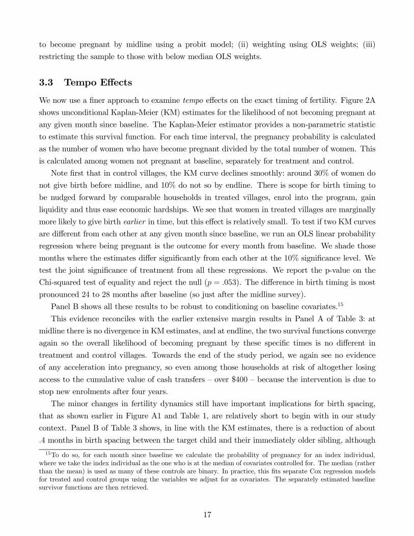
3.3 Tempo E¤ects

We now use a …ner approach to examine tempo e¤ects on the exact timing of fertility. Figure 2A

shows unconditional Kaplan-Meier (KM) estimates for the likelihood of not becoming pregnant at

any given month since baseline. The Kaplan-Meier estimator provides a non-parametric statistic

to estimate this survival function. For each time interval, the pregnancy probability is calculated

as the number of women who have become pregnant divided by the total number of women. This

is calculated among women not pregnant at baseline, separately for treatment and control.

Note …rst that in control villages, the KM curve declines smoothly: around 30% of women do

not give birth before midline, and 10% do not so by endline. There is scope for birth timing to

be nudged forward by comparable households in treated villages, enrol into the program, gain

liquidity and thus ease economic hardships. We see that women in treated villages are marginally

more likely to give birth earlier in time, but this e¤ect is relatively small. To test if two KM curves

are di¤erent from each other at any given month since baseline, we run an OLS linear probability

regression where being pregnant is the outcome for every month from baseline. We shade those

months where the estimates di¤er signi…cantly from each other at the 10% signi…cance level. We

test the joint signi…cance of treatment from all these regressions. We report the p-value on the

Chi-squared test of equality and reject the null ( = 053). The di¤erence in birth timing is most

pronounced 24 to 28 months after baseline (so just after the midline survey).

Panel B shows all these results to be robust to conditioning on baseline covariates.15

This evidence reconciles with the earlier extensive margin results in Panel A of Table 3: at

midline there is no divergence in KM estimates, and at endline, the two survival functions converge

again so the overall likelihood of becoming pregnant by these speci…c times is no di¤erent in

treatment and control villages. Towards the end of the study period, we again see no evidence

of any acceleration into pregnancy, so even among those households at risk of altogether losing

access to the cumulative value of cash transfers – over $400 – because the intervention is due to

stop new enrolments after four years.

The minor changes in fertility dynamics still have important implications for birth spacing,

that as shown earlier in Figure A1 and Table 1, are relatively short to begin with in our study

context. Panel B of Table 3 shows, in line with the KM estimates, there is a reduction of about

4 months in birth spacing between the target child and their immediately older sibling, although

15To do so, for each month since baseline we calculate the probability of pregnancy for an index individual,where we take the index individual as the one who is at the median of covariates controlled for. The median (ratherthan the mean) is used as many of these controls are binary. In practice, this …ts separate Cox regression modelsfor treated and control groups using the variables we adjust for as covariates. The separately estimated baselinesurvivor functions are then retrieved.

17

this is not statistically signi…cant. Birth intervals of less than 24 months are considered to place

the child at higher risk of mortality and undernutrition, and mothers with those intervals are

at a higher risk of birth complications [Pimentel et al. 2020, Damtie et al. 2021]. Focusing on

this threshold, we see there is a signi…cant increase of almost 5pp in such short birth spacing (in

controls, 123% of target child births are within 24 months of their older sibling). So there is some

heaping at this extreme threshold due to the responses of 5% of treated households.

The qualitative pattern of results on birth spacing are robust to: (i) conditioning on covariates

(right hand side of Table 3); (ii) weighting the sample in alternative ways (Panel B of Table A3).

3.4 Selection E¤ects

As a …nal step we examine whether there are changes in the composition of households becoming

pregnant over time – a selection e¤ect. This has not been studied much in the earlier literature,

but is not ruled out by the earlier null quantum e¤ects and muted tempo e¤ects: there could be

a compositional change in which households become pregnant even if aggregate fertility patterns

remain unchanged between treatment and controls.

Column 1 of Table 4 shows baseline characteristics of households, women, their husbands

and older sibling of the target child in control villages. We then show treatment e¤ects on that

characteristic among woman that became pregnant between: (i) baseline and midline (Column 2);

(ii) midline and endline (Column 3). In both time frames and for each and every characteristic –

of the household, the woman, her husband, or their older child – we …nd no evidence of signi…cant

selection e¤ects of treatment. Although some of these null impacts are imprecise, in most cases

the estimated standard error is less than 15% of the standard deviation of the same characteristic

among controls at baseline.

To examine dynamic selection, we check whether KM survival estimates di¤er along each

characteristic, between treated and control households. We take each characteristic and de…ne a

dummy equal to one if the household is above the median on that characteristic and zero otherwise

(or analogously for dummy variables). We then estimate the di¤erence-in-di¤erence in survival

functions. Column 4 in Table 3 reports the p-value on the null that this di¤erence-in-di¤erence

is zero, and the sign of this estimate in each case. There are only two characteristics for which

we …nd statistical evidence of dynamic selection e¤ects: (i) whether the woman can read and

write at baseline; (ii) whether she is rearing livestock as her primary income generating activity at

baseline. The sign of both di¤erence-in-di¤erences is negative, indicating that women that have

such characteristics signi…cantly delay selection into pregnancy relative to controls.

We return to these results in Section 5, as they relate to the nature of household decision

making and investment opportunities available to women, that helps explain why there are muted

impacts on fertility dynamics despite the o¤er of high-valued and long-lasting cash transfers.

18

4 Child and Mother Outcomes

The results so far address the question on whether the availability of high-valued unconditional cash

transfers to promote early childhood development has unintended impacts on fertility dynamics

among those not immediately eligible but who can later enrol into the program conditional on a

veri…ed pregnancy. We …nd null impacts of the intervention on the number, timing and selection

into birth, despite households having strong economic incentives to accelerate birth timing or

to have an additional child. To understand why this is so, we build evidence on the pattern of

marginal costs and bene…ts across household members from o¤er of cash transfers.

To begin with we examine how the intervention impacts outcomes of the target child and

their mother, conditional on any quantum, tempo and selection e¤ects. We compare outcomes to

those in Carneiro et al. [2021] that were based on women pregnant at baseline and so that did

not endogenously select to enrol into the intervention. This comparison helps con…rm whether

the muted impacts on fertility dynamics translate into equally sized treatment e¤ects for child

outcomes across the two samples, or whether these reveal potentially important unobservables

that at least determine selection into fertility (if not the incidence and timing of fertility choices

for treated households) and correlate to child and maternal outcomes.

4.1 Child Stunting and Health

We …rst examine the outcome of height-for-age Z-scores (HAZ) because this relates to stunting:

stunting is the best measure of cumulative e¤ects of chronic nutritional deprivation, and is recog-

nized as a key indicator of long-term well-being. To minimize measurement error, data on child

height was collected by a dedicated anthropometric enumerator in each survey wave.

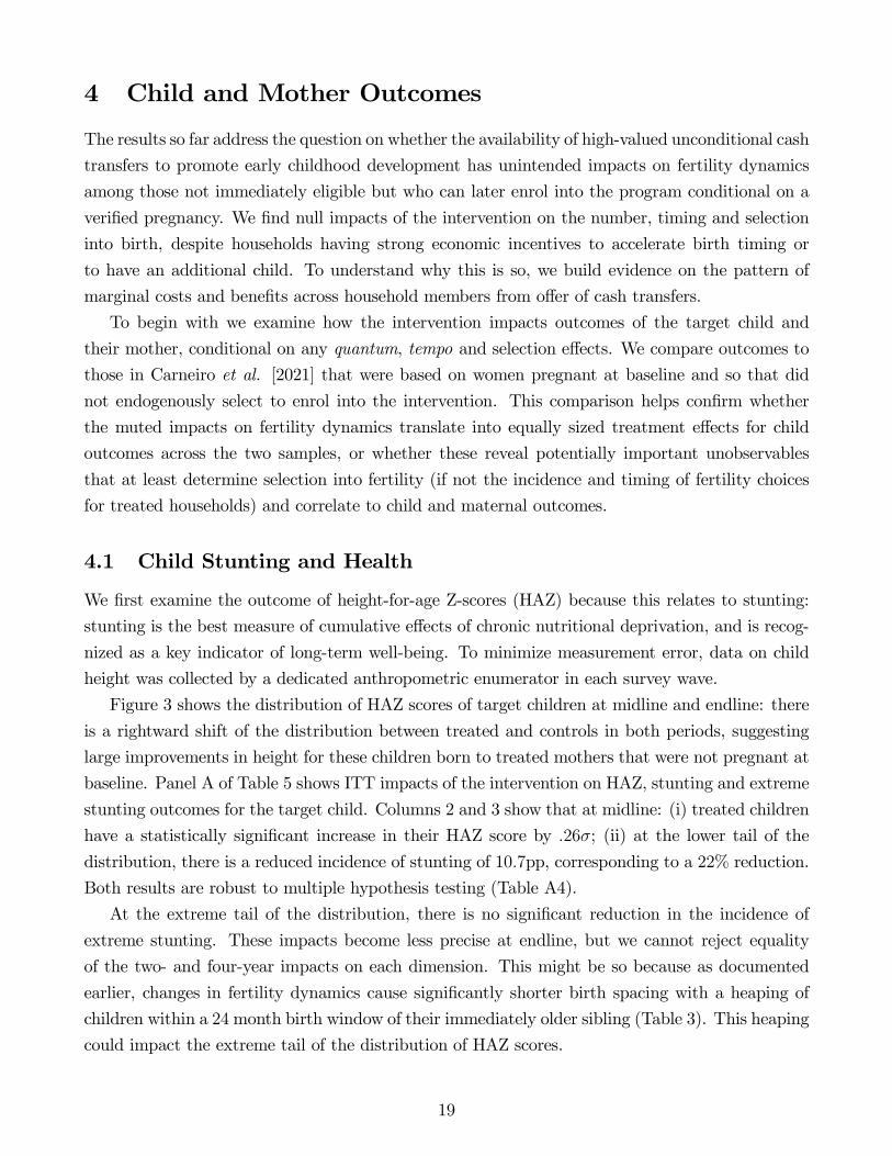
Figure 3 shows the distribution of HAZ scores of target children at midline and endline: there

is a rightward shift of the distribution between treated and controls in both periods, suggesting

large improvements in height for these children born to treated mothers that were not pregnant at

baseline. Panel A of Table 5 shows ITT impacts of the intervention on HAZ, stunting and extreme

stunting outcomes for the target child. Columns 2 and 3 show that at midline: (i) treated children

have a statistically signi…cant increase in their HAZ score by 26; (ii) at the lower tail of the

distribution, there is a reduced incidence of stunting of 107pp, corresponding to a 22% reduction.

Both results are robust to multiple hypothesis testing (Table A4).

At the extreme tail of the distribution, there is no signi…cant reduction in the incidence of

extreme stunting. These impacts become less precise at endline, but we cannot reject equality

of the two- and four-year impacts on each dimension. This might be so because as documented

earlier, changes in fertility dynamics cause signi…cantly shorter birth spacing with a heaping of

children within a 24month birth window of their immediately older sibling (Table 3). This heaping

could impact the extreme tail of the distribution of HAZ scores.

19

Columns 4 to 6 then repeat the analysis but for the target child born to women that were

pregnant at baseline. We see a very similar pattern of results, with endline impacts being more

precisely estimated in this sample (that is twice as large). Within each survey period, we cannot

reject equality of impacts across the two samples.

One concern is that the earlier tempo e¤ect results suggested small changes in birth timing (that

were not robustly di¤erent between treatment and controls). As a result, at midline the target

child is 12 months old in control villages, and 11 months old in treated villages; at endline the

target child is 35 (34) months old in control (treated) villages. To establish these small di¤erences

in age do not drive any of these results for height, Table A5 shows these estimates are robust to

non-parametrically controlling for the age of the target child at midline and endline.

Panel B of Table 5 shows treatment e¤ect estimates on health-related outcomes for the target

child, again split between those born to women not pregnant at baseline (Columns 1 to 3) and

those born to women pregnant at baseline (Columns 4 to 6). We …rst consider an index of health

outcomes made up of two dummy variable components: whether the new child has not been

ill in the last month, and whether the target child had diarrhea in the two weeks prior to the

survey. Among target children born to women not pregnant at baseline, this index signi…cantly

improves by 16 at midline, and by 21 at endline (where this latter result remains robust to

multiple hypothesis testing). The remaining rows show impacts on each index component: there

is a reduction in illness/injury for new children of 6pp at midline, and this reduction improves

slightly to 96pp (corresponding to a 15% fall relative to controls) by endline. The incidence of

diarrhea among the target child also falls dramatically: at midline there is a reduction of 58pp,

and this falls further by 84pp (corresponding to a 24% fall) at endline.

The right hand side of Panel B shows a very comparable set of e¤ects in the sample of target

children born to women that were pregnant at baseline. Again, within each survey period, we

cannot reject equality of impacts across the two samples.

If households were endogenously responding to the o¤er of cash transfers by bringing forward

the timing of births, the most important marginal cost of doing so would be to worsen child

outcomes – especially given birth spacing is below WHO recommendations to begin with. These

results establish there is no such evidence of such impacts on children of mothers that were not

pregnant at baseline.

4.2 Dynamic Treatment E¤ects

We noted above that for women not pregnant at baseline, the average age of their target child is 11

(34) months at midline (endline). Outcomes for the target children of women that were pregnant

at baseline are measured when they are aged around 24 (48) months at midline and endline

respectively. Hence we can collate the estimates across samples to show dynamic treatment e¤ects

on children approximately aged 1, 2, 3 and 4 years. Figure 4 shows these dynamic treatment

20

e¤ects for each outcome. We see they are monotonic across these four age bands: the intervention

has reduced impacts on HAZ over time, while there are accumulating impacts on child health.

In short, the trajectory of child development is very similar between the children born to

women that were, or were not, pregnant at baseline. An immediate implication is that the IRR

to the program, in terms of child outcomes, is likely to be similar to that calculated in Carneiro

et al. [2021] for the sample of households in which women were already veri…ed to be pregnant

at baseline. Under plausible assumptions that was calculated to be at least 10%. Given high

fertility rates in this setting, these gains accrue not just to the cross section of women that happen

to pregnant at baseline, but also to a further 90% of women aged 12-49 at baseline that become

pregnant over the four year window of the program.

The only clearly non-monotonic outcome is extreme stunting. Again this might be because

of the small share of treated households that change fertility timing to cause a heaping of birth

spacing of the target child within a 24 month birth window of their immediately older sibling.

Taken together, the results con…rm the muted impacts on fertility dynamics translate into

equally sized treatment e¤ects for child outcomes across the two samples. The largely monotonic

results across samples help ameliorate the concern that unobservables drive the exact timing and

selection of treated households into fertility among those that were not pregnant at baseline.

4.3 Maternal Outcomes

The other key marginal cost of bringing forward birth timing to the o¤er of unconditional cash

transfers is to worsen maternal health. By examining such outcomes we address a broader concern

that the majority of early childhood evaluations lack detailed analysis of maternal outcomes beyond

those related to parenting practices [Evans et al. 2021]. Moreover, it has been documented in

a similar setting that husbands might be ill-informed about maternal mortality and morbidity

compared to their wives [Ashraf et al. 2020a]. If fathers have some say over birth timing and are

less aware of these marginal costs of bringing forward births, this could tilt the balance towards

such endogenous responses to the o¤er of cash transfers in our setting.

The results are in Table 6, where Column 1 shows baseline outcomes for women not pregnant

in control villages. Columns 2 and 3 show that on weight, height, BMI and an indicator for

malnourishment, there is no evidence of worsening health outcomes for mothers, either at the two-

year midline or four-year endline. The right hand side of the table replicates …ndings from Carneiro

et al. [2021] to show the same outcomes for mothers pregnant at baseline and so exogenously

eligible for the cash transfers. We see that the pattern of null impacts is the same in both samples.

Within each survey period, we cannot reject equality of impacts across the two samples.

This further underpins the earlier results that there are precise null endogenous fertility re-

sponses to the intervention, so that there are no hidden marginal costs in terms of maternal health

from any response of non pregnant women to the intervention o¤er of cash transfers.

21

5 Explaining the Lack of Fertility Responses

Our study context is one in which the presence of a new intervention o¤ering high-scale and long-

lasting unconditional cash transfers to pregnant women, there are strong economic motivations

for households to bring forward the timing of births to obtain receipt of those resources, and help

alleviate economic hardships faced. Yet we …nd very muted impacts on total fertility, the timing

of births or selection into births. All these results are buttressed by pattern of child and maternal

outcomes being in line with those found for mothers already pregnant at baseline and so who could

not endogenously enrol into the program.

To begin explaining this null response, we …rst note that given the near complete absence of

contraceptive availability in this region, women have less agency over fertility timing relative to

contexts in which contraceptives (especially those controlled by women) are available. Moreover,

Nigeria is a patriarchal society where bridal prices are still common, so wives are often perceived as

being purchased by their husbands. This leads to decisions about reproduction residing primarily

in the hands of the husband and his family, as is well documented by work in demography and

gender studies [Caldwell and Caldwell 1987, 1988, Odimegwu and Adenini 2014, 2015].16

Furthermore, the primary marginal costs of accelerating birth timing are likely borne by moth-

ers through risks in pregnancy and to their later health. Hence given the wedge between wives –

who primarily bear the marginal costs of shifts in birth timing or total fertility – and their hus-

bands, who largely drive fertility decisions given the absence of contraceptives, we dig deeper into

the nature of intrahousehold decision making and women’s agency, to establish how the marginal

bene…ts of receiving cash transfers are distributed among household members.

5.1 Decision Making

To begin with, we consider decision making rights over other dimensions beyond fertility. Using

a comparable sample as our evaluation sample, the 2013 DHS Nigeria data suggests husbands

have decisive decision making rights over many outcomes a¤ecting their wives beyond fertility

– including health care, the purchase of large household items, and being able to visit family

members. For example, when asked how decisions are made on these dimensions, the share of

women that report their husband decides alone is, 91% for the health care of the woman, 93% for

the purchase of large household items, and 75% for visits to family members.

However, the DHS data show there is one key dimension on which wives retain agency: how to

16The evidence on the causal impact of a greater availability of contraceptives on fertility is mixed. A small setof experimental studies, discussed in Ashraf et al. [2014], provide mixed results: increasing access to contraceptionis found to have a signi…cant impact on decreasing fertility in four countries: Ghana, Tanzania, Bangladesh andColombia. No impact is evident in Ethiopia, Indonesia, Uganda and Zambia. Miller et al. [2021] use a structuralmodel to estimate impacts on contraceptive use of eliminating supply constraints using a sample of DHS countriesin Sub Saharan Africa. They reach the conclusion that eliminating supply constraints would have limited impactson contraceptive use, while policies targeting husbands beliefs and preferences could be more e¤ective.

22

spend their earnings. In sharp contrast to other dimensions of decision making, over 90% report

of women report they alone choose how to spend money they bring into the household.

We designed our baseline survey module on household decision to follow the structure of the

DHS questions. Our data largely corroborates this sharp contrast in agency women have over

earnings versus other dimensions of household decision making. Figure 5 shows data from our

baseline survey on household decision making over various dimensions. On each dimension, the

top bar shows women’s report over who in the household makes decisions, and the bottom bar

shows the corresponding report of husbands (where recall, we interviewed spouses separately).

In line with DHS data, our survey reveals women have weak decision making rights over major

household purchases, which food to grow, and what food to buy. As the top half of Figure 5

shows, along all three dimensions, the majority of women report their husband decides alone (or

in consultation with them); very few women ever make these decisions alone. These …ndings are

con…rmed in both interviews to the wife and their husband.

However, we additionally asked a series of vignette questions on who would have decision

making rights over any new ‡ow of resources that the wife generated. Recall, that as shown in

Table 1, in our sample women have high labor force participation rates, and so the majority will

normally be bringing a ‡ow of earnings into the household. Our vignettes varied: (i) the source of

women’s earnings, contrasting between labor market earnings obtained through selling snacks – a

common form of self-employment for women, versus if the money were received as a gift; (ii) the

amount of monthly earnings gained, contrasting NGN3500 (to match the value of monthly cash

transfers from the CDGP), to the receipt of NGN1000.

As shown in the lower part of Figure 5, in each of these scenarios: (i) the majority of women

reported they would decide alone how to spend the additional resources; (ii) this was irrespective

of how the additional resources were generated (either through labor earnings, or as a gift to the

wife) or the amount of additional earnings; (iii) husband reports were near identical to their wives.

5.1.1 Decision Making over Unconditional Cash Transfers

Building on this insight that both spouses report women controlling any additional resources they

bring to the household, we next zoom in to consider who in the household decides how to spend

the actual cash transfers from the intervention. The question reported in the bottom set of bars

in Figure 5 was asked at midline in treated villages: we asked each spouse about who actually got

to decide how the unconditional cash transfer from the CDGP program was spent. Even more

so than the hypothetical positive earnings shocks asked about, in over 70% of households women

report being able to decide alone over how the unconditional cash transfer is spent. This is entirely

corroborated with what husbands themselves report.

Taken together, the results in Figure 5 show household decision making is well characterized

within a separate spheres framework [Lundberg and Pollak 1993, Browning et al. 2010]: while

23

nearly no women have access to family planning and men thus can have relatively more control

over the timing of fertility, the reverse is true for the control of the cash transfers received from

the intervention. This creates a wedge between the private returns to the receipt of cash transfer

between women and their husbands.

In order to understand exactly what men gain on the margin from the receipt of cash transfers

within their household, we document how women use these resources.

5.2 How Unconditional Cash Transfers are Spent

Descriptives Figure 6 presents descriptive evidence on how, at midline and endline, women

report spending the unconditional cash transfers. It is again instructive to show comparable

results among women that were pregnant at baseline, and so did not endogenously choose to

become eligible for cash transfers. Throughout we see little di¤erence between the spending

patterns of these two groups. The majority of women report spending the cash on food for the

household (that slightly declines between midline and endline), for food for children (that rises

between midline and endline as expected as children age), and on assets (that rise between midline

and endline).

In the remainder of this Subsection, we present ITT estimates, using the speci…cation described

in (1), of how additional resources are spent in terms of consumption, savings, and own business

investments. This builds up a granular picture of the marginal gains to husbands from bringing

forward the timing of births in order for the additional resources from the intervention to ‡ow

into their household. To be clear, husbands might well value gains of improved child outcomes

to the exact same extent as their wives. However, given the majority of households give birth at

some point over the four year period the intervention is announced to be in place for, these gains

would accrue irrespective of whether birth timing was brought forward or the household retained

its original fertility path when the program is …rst announced. Hence we focus on other material

gains resulting from the receipt of the cash transfers. Some of these gains will be shared with

other household members – such as building a bu¤er stock of savings, but others will be closer to

private gains to the husband in terms of expenditures on certain adult goods or investments into

the husband’s labor activities.

Consumption, Adult Goods and Food Security Table 7 presents treatment e¤ect estimates

on how the additional resources are used, focusing …rst on consumption and savings. The …rst

row on Panel A examines two- and four-year impacts on monthly food expenditures (calculated

based on a seven-day recall and aggregated over food groups). Food expenditures rise in treated

households by $26 (31%) over controls at midline, and this is largely sustained at endline where

they are $19 higher than controls. Some of these increases will of course bene…t husbands. However,

given that household sizes are over seven at baseline (before the birth of the target child), the

24

equivalized share of food expenditure accruing to husbands will likely be a relatively small share

of the original value of the cash transfer.

The next two rows examine this further by focusing on impacts on the extensive margin of non-

food expenditures for male-orientated adult goods: tobacco/cigarettes, and newspapers/magazines.

We see that neither type of adult good expenditure increases (indeed expenditures on ciga-

rettes/tobacco might even be less likely to occur in treated households). The next row shows

no signi…cant rise in monthly non-food expenditures overall, although these estimates are noisier

than for food expenditures.17

Panel B then examines outcomes related to food security: we see that at baseline in controls,

30% of households report not having enough food to eat in the past year. In this region the

agricultural cycle includes a lean season from March to October in which households face food

shortages, and have to resort to extreme coping strategies. We see that in treated households food

security improves dramatically by endline, with a 14pp fall in households not reporting having

enough food to eat (a result robust to multiple hypothesis testing). The rows below show these

longer run improvements in food security are concentrated in lean season months. These clearly

are long run bene…ts that accrue to all household members from being able to smooth consumption

as a result of gaining access to the cash transfers from the intervention.

Saving As described in Carneiro et al. [2021], there are two substantive reasons why the cash

transfers can impact outcomes beyond consumption. First, the value of the cash transfer was

calibrated by our intervention partners to correspond to the cost of a diverse household diet.

However, at baseline controls already spend $83 per month on food suggesting a potential crowd

out of resources for other uses. Second, the fact that transfers are provided each month until

the target child is 24 months old, provides women with a more stable ‡ow of resources than is

available from most labor activities in these rural economies. The magnitude and certainty of

transfers opens up the possibility that they are used for saving and investment purposes, over and

above impacts on consumption.

We begin to examine these other outcomes in Panel C of Table 7. This presents ITT estimates

on household savings. By endline there is a signi…cant rise in the stock of household savings of $56

(22%), equivalent to 25 months of cash transfers (a result robust to multiple hypothesis testing).

This bene…ts husbands in allowing their household to build resilience to shocks.

Taken together, these results show the gains to husbands from their wife receiving the cash

transfer are either relatively small (in terms of food and non-food expenditures), concentrated

during the lean season (in terms of food security at endline), or accrue some time into the future

17Non-food expenditure is obtained combining the following sources: (i) a 7-day expenditure recall of consumables(e.g. matches, fuel); (ii) a 30-day recall of other items (e.g. toiletries, utensils, household items, health expenditure);(iii) a 12-month recall of major expenses (e.g. school fees, ceremony costs, remittances); (iv) expenditure on durablesusing a 12-month recall of expenditure on assets the household owns (e.g. TV set, wheelbarrow, mattress). Thetop 1% of total expenditure amounts are trimmed.

25

(in terms of accumulated savings by endline).

Labor Activities and Investment into Own Businesses Cash transfers can also be used

to advance the labor activities of wives and husbands. We narrow in on impacts speci…c to each

partner to shed light on the private gains to men from their wife being in receipt of cash transfers,

beyond the impacts on food expenditure, food security and savings shown above.

These results are shown in Table 8. Panel A …rst focuses on labor activities each spouse is

engaged in. Women’s labor force participation rates are high to begin with (72% at baseline in

controls). For treated women this rises by a further 9pp by endline (a result robust to multiple

hypothesis testing). The right hand side shows much smaller impacts on husband’s labor supply.

On the types of labor activity engaged in, at baseline the most common activities for women

are being self-employed in rearing livestock or petty trading. For women, by endline we see

signi…cant increases in any form of self-employment, and in petty trading activities. These are

large magnitudes of impact of engagement in these forms of self-employment, corresponding to 23%

and 32% increases respectively. It is perhaps unsurprising that these impacts are not immediate

or measured at the two-year midline given our sample of women are not pregnant at baseline, but

the majority give birth to the target child by midline (Figure 2).

The right hand side of Table 8 shows no corresponding impact on the labor activities of

husbands: they are mostly engaged in farming their own land and the incidence of this does not

change post-intervention.

In Panel B we examine investments into the self-employment business of wives and their hus-

bands separately. Given women’s main form of self-employment in this context, we consider

business investment and livestock ownership. We see that both types of productive investment

signi…cantly increase by endline. On inputs into women’s businesses, these increase signi…cantly

by $20/month at endline. We see no corresponding increase in expenditures on inputs for the

husband’s business. Regarding livestock ownership, women’s ownership of any animal increases

by 69pp (9%) at midline, and by 102pp (13%) at endline. Livestock ownership is critical in this

economic environment because it raises mean earnings for women from the sale of animal produce

such as milk and eggs, and it produces an earnings stream all year round thus reducing women’s

volatility of earnings.18

The …nal row of Table 8 combines all the information on changes in labor activity to construct

a (noisy) measure of total monthly earnings from all forms of employment, for each spouse. We see

that by endline, women’s earnings increase by $173 (corresponding to a 19% rise over the baseline

level in control villages). In line with all the earlier results, we see no statistically signi…cant

impacts on earnings of husbands, either at midline or by endline.

18As in Carneiro et al. [2021] we note that in this setting livestock are owned by an individual (not a household).Examining livestock ownership of women that were not-pregnant at baseline we …nd: (i) signi…cant increases inhousehold ownership of livestock are largely driven by livestock owned by treated women (and not another householdmember); (ii) the ITT point estimate on them owning any given animal is higher at endline than midline.

26

In summary, there are sharply divergent gains across spouses in terms of their labor activities,

own business assets, and earnings as a result of the household becoming eligible for the cash trans-

fers from the CDGP intervention. These cash transfers are provided directly to women, and then

data suggests women retain the agency to spend these resources to push forward transformative

changes in their labor supply, self-employment and the accumulation of productive assets for their

own businesses.

This pattern of results on the use of cash transfers is also borne out in the parallel qualitative

analysis of the CDGP conducted in our study context [Sharp et al. 2018]. This shows women

invested into small-scale home-based activities such as petty trade, food processing and sale, small

livestock rearing, and services to other women (such as hairdressing or pounding grain). The

qualitative analysis also …nds that while bene…ciaries do give cash gifts out of their transfer to

their husbands, these are small and one-o¤ transfers. The largest recorded in the qualitative

sample was NGN1100, so less than one third of one month’s transfer.

A growing literature on micro-entrepreneurship in developing countries has shown that male

but not female-operated enterprises bene…t from unconditional cash transfers. A number of expla-

nations have been put forward for this: (i) women are subject to expropriation by husbands [de

Mel et al. 2009, Jakiela and Ozier 2016]; (ii) women are less committed to grow their enterprises

or are more impatient [Fafchamps et al. 2014]; (iii) women sort into less pro…table sectors because

of unequal labor market access/preference for ‡exibility [Bernhardt et al. 2019]. None of these

appear to apply in our context because our evidence suggests women critically: (i) retain control of

resources; (ii) have pro…table business investments to undertake; (iii) opt not to transfer resources

to their husbands for their consumption of adult goods or own business investments.

5.3 Separate Spheres

A granular picture emerges where the private gains to husbands from bringing forward the timing

of births are limited to any share of food consumption that accrues to them, and enabling their

households to be more food secure and build a bu¤er stock of savings by the four-year endline.

They do not gain in terms of expenditures on adult goods, their labor activities or associated

business investments. In short, the muted response to the o¤er of high-valued and long-lasting

cash transfers can follow from the fact that ultimately, men have weak private material incentives

to shift forward the timing of births. This is despite households residing in extreme poverty, and

so having short term need for …nancial liquidity and longer term needs for economic resources.

These patterns of behavior are inconsistent with a unitary model of household decision making,

and more closely mimic separate spheres decision making between spouses. However, we make no

claim as to whether households reach the frontier of their production possibility set. For example,

in households where the marginal return to the husband’s own business investment was higher than

for their wife, on face value it would seem that household surplus would have been maximized if the

27

wife transferred resources to him to make those investments. However, this calculation implicitly

holds constant family size. If husbands anticipate such ex post transfers, then in treated villages

they have greater ex ante incentives to endogenously bring forward birth timing, and it is thus

unclear whether this leaves wives better o¤ overall given they bear the cost in terms of maternal

health as a result of shortened birth spacing.

We reiterate that in this context, women’s labor force participation rates are high, with most

women engaged in self-employment activities, and many having productive investments they can

make in their own business. This links back to the earlier results on dynamic selection (Table 4)

where we found evidence that wives that signi…cantly delayed selection into pregnancy in treated

villages relative to controls had two characteristics: (i) they could read and write; (ii) they were

rearing livestock as a primary income generating activity at baseline. Both results are consistent

with those women having productive investments available to them (either because they are skilled

or want to build their livestock asset base). Hence, all else equal, in these households, the private

incentive of husband’s to bring forward the timing of fertility is relatively weak.

We underpin this interpretation by considering within-sample variation in fertility responses.

We consider women that at baseline have a constellation of three characteristics: (i) they report

having full autonomy over how to spend any exogenous increase in resources they bring into the

household; (ii) they are self-employed; (iii) and, they have opportunities for business investment

(either because they own livestock or have business assets). We consider households in which,

at baseline, wives have all three of these characteristics versus households in which wives do

not have all three conditions satis…ed. Under separate spheres household decision making, we

view the former group of households as ones in which husbands have relatively weaker incentives

to bring forward birth timing, and the latter as ones in which husbands have relatively stronger

incentives to do so – either because they can appropriate the resources from the CDGP intervention

(condition (i)), or their wife transfers resources to them because she lacks investment opportunities

of her own (conditions (ii) and (iii)). With this classi…cation, 414 (815) households are ones in

which the husband has weak (strong) incentives. Naturally those households classi…ed as having

stronger incentives are more heterogenous because they include those for whom none, one or two

of conditions (i) to (iii) are satis…ed.

The results on quantum e¤ects on fertility in these subsamples are shown in Panel A of Table 9.

Columns 1 to 3 show that in households in which the husband has weaker incentives, we continue

to …nd null impacts on whether any child is born between baseline and the two-year midline, and

between midline and the four-year endline. Similarly, we continue to …nd no statistically signi…cant

impact on the number of children born over these time periods. These null impacts remain precise.

For example on the number of children born, we note the standard error from Column 3 is less

than 13% of the standard deviation of the outcome in controls. The 95% con…dence intervals

rule out a treatment e¤ect on the number of children born larger than 151 between baseline and

midline, and larger than 176 between midline and endline.

28

These results are in contrast to those for households in which the husband faces relatively

stronger incentives to bring forward the timing of births, shown in Columns 4 to 6. We see that

among this group, treated households are 92pp signi…cantly more likely to have any children born

between baseline and midline (corresponding to a 16% increase over comparable households in

controls), and to have 08 more children born over the same period. As is intuitive, this increase

in fertility occurs within the …rst two years of the program being introduced.

Pooling speci…cations and testing for di¤erences across households where husbands have weaker

and stronger incentives, the di¤erential impact on the number of children born between baseline

and midline is statistically di¤erent ( = 091).

On the tempo e¤ects or exact timing of births, Figure 7 shows unconditional Kaplan-Meier

(KM) estimates for the likelihood of not becoming pregnant at any given month since baseline, split

by these subsamples. Panel A shows that among those with relatively weaker incentives, there is

no di¤erential pattern of birth timing between treatment and controls in any month since baseline.

In contrast, Panel B shows the timing of fertility among those with relatively stronger incentives to

bring forward birth timing, in treatment and control villages. We see that those in treated villages

signi…cantly bring forward birth timing, with the most pronounced e¤ects occurring around the

two-year midline, and just prior to the end of the intervention at endline (where we shade in gray

the months since baseline where the KM curves signi…cantly di¤er).

Completing the analysis of tempo e¤ects, Panel B of Table 9 shows that within the subsample

of households where husbands have weaker incentives to bring forward birth timing,we also see

null impacts on birth spacing consistent with our core …ndings. For those with stronger incentives,

we do not however see any signi…cant reductions in birth spacing between the target child and

older sibling suggesting that even within this group those that endogenously respond to the o¤er

of cash transfers do so in a way so that any marginal costs of bringing forward birth timing do

not worsen child or maternal outcomes.

5.4 Alternative Explanations

We consider four alternative explanations for the null impacts on fertility. Each is unrelated to

separate spheres household decision making and thus any distinct role for husbands and wives.

Birth Spacing Households might be unable to bring forward birth timing if they are already

close to the lower biological bound on birth spacing. As shown in Table 1, at baseline our sample

households are characterized by having high fertility rates and short birth intervals. However, we

also see that the median birth spacing between the new child and their immediately older sibling

is 31 months, so it remains feasible for households to shorten further the birth interval between

the target child and their older sibling. Households are also not at the end of their fertility cycle.

As Table 1 shows, the average number of children at baseline is four, while DHS data reported

29

in Figure A1 suggests total fertility rates are close to six in this region. To probe this further,

Columns 1 and 2 of Table A6 show the estimated incentive e¤ects when we split the sample into

women with above/below the median number of children at baseline: we …nd a very similar pattern

of null impacts on the number and timing of births in both.

Polygamy 40% of our sample households are in polygamous marriages (Table 1). Null e¤ects

might then be driven by husbands having small returns for bringing forward birth timing for any

given wife. Two factors mitigate against this interpretation. First, in polygamous marriages any

wife that is pregnant is eligible for the CDGP transfers (not just one wife). Second, Columns 3

and 4 of Table A6 estimate e¤ects on fertility by polygamous and non-polygamous households:

we …nd very similar (and equally muted) responses in fertility dynamics.

Policy Certainty A third explanation is that households expect the o¤er of cash transfers from

the intervention to be available for the foreseeable future. Given transfers are only available for

one child, and fertility rates are high to begin with, households might be secure in the knowledge

that they will eventually receive the transfers without having to adjust their planned fertility path.

Two pieces of evidence mitigate against this interpretation.

First, this is an environment in which state or NGO capacity to reliably deliver programs is

generally limited, and households face huge uncertainties from aggregate shocks, both natural and

man made. This applies to all …ve LGAs in the states of Zamfara and Jigawa in our evaluation

sample. We described earlier how village insecurity led to our enumerators being unable to reach

some villages. Figure A4 shows that even in the secure villages that form our sample, nearly all

have been hit by a natural shock in the year prior to midline or endline (such as crop damage

caused by weather or pests, ‡oods and droughts), and with the majority having been hit by a

man made shock (such as curfews, violence, or widespread migration into the village). With such

background uncertainty, households might perceive a relatively narrow prospect of cash transfers

being delivered for the full four year intention originally announced, again providing incentives to

bring forward the timing of births.

Second, the CDGP intervention did not last forever and this was known to households. As the

timeline in Figure 1 shows, the program stopped enrolling pregnant mothers in April 2019, around

six months after our endline survey (women who were veri…ed to be pregnant before that deadline

would still be eligible for the full sequence of monthly cash transfers until their child turned 24

months old). This announcement was made just before our endline survey began to be rolled out,

allowing us to measure whether households were aware of the termination. Although knowledge

was far from perfect, we …nd that at endline, among women in treated villages: (i) 68% correctly

knew how long they could expect to receive cash transfers for; (ii) 67% correctly stated the year in

which the CDGP would end; (iii) 59% heard this information directly from community volunteers

charged to disseminate the information component of the intervention.

30

Moreover, the KM estimates in Figure 2 show no spike in births towards the endline survey

being triggered by the announcement. Households that have not become pregnant at that stage

risk losing cash transfers altogether. At the four-year endline, 94% of households in treated

villages that have a non-pregnant woman in them at baseline, still have not had a child by endline

(and this does not di¤er to controls where it is 99%).19

Time Lags A …nal explanation for the null fertility impacts relates to the fact that women only

become eligible to receive cash transfers once their pregnancy is veri…ed via a urine test. This

usually occurs in the second or third trimester of pregnancy. Hence there is obviously some lag

between when a household might …rst decide to respond to the o¤er of cash transfers and their

actual receipt. Null fertility impacts could then result because this time lag causes any marginal

bene…t to bring forward birth timing to be discounted. However, the fact that as shown in Table

9 there does exist a subset of households that do respond on the fertility margin suggests such

time lags are not su¢cient to explain our core results in the sample overall.

As a further check on this, we consider responses among households with above/below median

savings at baseline, as a potential proxy for those with higher/lower discount rates: the results in

Columns 9 to 12 of Table A6 show both sets of households have largely null response in terms of

total fertility (Panel A). Those with low savings at baseline appear to be among those contributing

to a heaping of birth spacing below 24 months for the target child (Panel B).

We return to this issue of time lags below when considering policy implications of our …ndings.

6 Discussion

We conclude by discussing the external validity of our …ndings, and their policy implications for

the next generation of interventions designed to use cash transfers to promote human capital

development in early childhood in low-income contexts.

6.1 External Validity

The null e¤ect on fertility dynamics in our study can be explained by a constellation of three factors

in our context: (i) there is separate spheres decision making, women retain control of resources

they bring into the household, including how cash transfers from the intervention are spent; (ii)

women have high labor force participation rates and have productive investment opportunities

available to them through their own businesses; (iii) women prefer to invest in these opportunities

rather than make intrahousehold transfers to husbands. These factors combine to imply husbands

have little private incentive to change fertility dynamics in response to the program.

19We also note that the value of the cash transfer increased from NGN3500 to NGN4000 from January 2017.Again we see no evidence from Figure 2 that this marginal increase in …nancial incentives changed fertility dynamics.

31

The external validity of our …ndings hinge on how peculiar this constellation of factors is.

We investigate this by drawing together DHS surveys from 45 middle and low-income settings to

document the prevalence of these factors, as closely as can be measured in a large cross-country

sample (and combining rural and urban samples). In doing so, we shed light on which developing

country contexts are more or less likely to see unintended fertility consequences when substantial

cash transfers for early childhood development are o¤ered to pregnant mothers. The results are

in Figure 8.

Panel A examines the prevalence of separate spheres decision making: it shows a scatter plot

of the share of married women that report using any form of contraception, against the share

of women that report being able to decide how to spend their own earnings. The vertical and

horizontal lines represent the means of the variable stated on each axis, splitting the …gure into

quadrants based on being above/below each mean. Countries with separate spheres decision mak-

ing as in the CDGP sample lie in the South East quadrant (orange dots). This is not uncommon:

Nigeria lies within a cluster of such countries, that also includes Ghana, Niger, Uganda and the

Gambia for example.

Panel B shows a scatter plot of employment rates for married women (that includes self-

employment) against the share of women that report being able to decide how to spend their

earnings. To link to the scatter on separate spheres decision making, we use the same color coding

as in Panel A. Those countries in the North East quadrant have higher than average female

employment rates and women control how to spend their earnings. Somewhat surprisingly, most

countries in this quadrant (9 out of 16) have separate spheres decision making (orange dots). These

include Nigeria, but also Ghana, Gambia, Uganda and Burkino Faso. It is in such countries where

the same constellation of factors come together as in our evaluation sample, and, all else equal,

we might then expect relatively muted (unintended) consequences on fertility dynamics from the

o¤er of high-valued and long-lasting cash transfers to pregnant women.

Concerns over unintended fertility consequences will be stronger in countries where fertility

and spending decisions are in the hands of the same spouse: in Panel A these are in the North

East quadrant (women control both, brown dots) and South West quadrant (husbands control

both, green dots). Panel B shows that among countries where women control both decisions,

nearly all have higher than average female employment rates too. In these contexts, women can

best internalize any cost of bringing forward birth timing, they retain control of cash transfers and

have productive investments they can make related to employment opportunities.

Among countries where husbands control both decisions (green dots), there is far more variation

in employment rates for women. Among those in the North West quadrant of Panel B, there at

least remains the option of husbands opting to invest cash transfers in the employment prospects

of their wife. These countries include Burundi, Liberia and Tanzania. For those in the South

West quadrant of Panel B, women lack labor market opportunities and so might well lack even

the possibility of using cash transfers to make productive investments. These countries include

32

Ethiopia and Mozambique. Outside of Sub Saharan African, these countries include Afghanistan

and Tajikistan. These are locations where our results suggest the most caution when using cash

transfers to promote early childhood development.20

6.2 Policy Design

We end by discussing design issues to consider in the next generation of interventions using cash

transfers to promote child outcomes in early life. We consider design margins related to targeting,

eligibility and component bundling.

Targeting It matters who in the household cash transfers are provided to. Most conditional

cash transfer programs in developing countries explicitly target payments to women [Fiszbein and

Schady 2009]. A few studies have experimentally varied the identity of recipients in the household,

with mixed …ndings: while some studies suggest targeting women can change consumption levels

and bundles [Armand et al. 2020], other studies …nd less impact [Benhassine et al. 2015, Haushofer

and Shapiro 2016]. Our results suggest targeting resources to women rather than husbands will

be especially important for avoiding unintended fertility impacts in contexts where women control

the use of any additional earnings and have productive investment opportunities available to them.

Eligibility The purpose of eligibility being linked to pregnancy is so that bene…ts start accruing

to the child as early as possible – even while they are in utero as in the CDGP. However, in

contexts where unintended fertility consequences might occur, policy makers could ease the concern

by further separating in time when fertility decisions are made and when payments start to be

received. This leads to a policy trade-o¤: having payments start later (perhaps when the child

is born or sometime later within the …rst 1000 days of life) will lower potential impacts on child

outcomes, but at the same time could prevent a rush to bring forward births, and this force moves

to improve children’s initial outcomes such as birthweight, as well as impacting maternal health.

On component bundling, consider …rst information plus cash designs. In our context infor-

mation was provided as a public good. Hence there was no reason to change fertility dynamics

in order for households to gain from that component of the program. However, designs where

information components are more targeting to speci…c households – say because of the desire to

provide tailored information to mothers – do potentially create a second incentive for households

to bring forward birth timing. Again, policy makers face a trade-o¤ between improving child

outcomes through more household-speci…c information delivery, versus worsening child outcomes

through accelerated fertility and shorter birth intervals.

20Our analysis of DHS data also helps explain the …ndings of Palermo et al. [2016], who study a child grantprogram in Zambia and also …nd null impacts on fertility. As Panel A shows, Zambia is a context where a highshare of women report using contraceptives and so can exert more control over the timing of births. As such theyare better able to internalize any marginal cost of accelerating birth timing.

33

Component Bundling It might be natural to think of also providing family planning to women,

or to empower them through the provision of bargaining and negotiation skills [Ashraf 2009, Ashraf

et al. 2014, 2020b]. However, it is unclear what impacts this would have for the timing of births

relative to the counterfactual of existing decision making rights. It might break the delicate

balance of separate spheres decision making in some contexts, but in other contexts, it would

allow women to internalize the costs and bene…ts of bringing forward the timing of births, while

retaining control over earnings streams.

7 Conclusion

Huge reductions in global poverty have been achieved over the last three decades, at least until

the global COVID-19 pandemic. Some part is due to the increased use of direct transfers to the

poor. Such transfers have been a key policy response to the pandemic in low-income countries,

and as such seem destined to become entrenched as a policy instrument in the developing world.

As the spread of these programs coincides with renewed policy interest in fostering human capital

accumulation in early life, policy makers are increasingly targeting cash transfers to pregnant

mothers or those with young children, with this aim. We have provided granular evidence on any

causal distortionary e¤ect that such conditionality – based on veri…ed pregnancy – provides on

fertility behaviors. In a context where households face extreme economic hardships, we show such

unintended consequences are avoided – even with the o¤er of high-valued cash transfers – where

there exists a constellation of three factors: (i) women retain full control over the use of transfers

they bring into their household; (ii) women have available productive investment opportunities in

their own businesses; (iii) they choose to transfer few resources to husbands.

Given these forces, that are not unique to our context, an important implication is that the

Child Development Grant Program we study has widespread bene…ts across households: both the

cross section of those exogenously enrolled into the program because they contain a pregnant

woman at baseline, and the far larger group of households that endogenously enrol through preg-

nancy over the lifetime of the intervention. By setting out a precise mechanism driving the lack

of distortionary e¤ects, we are able to speculate on parts of the developing world where similar

programs can be expected to generate high population-wide returns, and also settings where more

caution needs to be taken in the design of cash transfers promoting early childhood development.

Finally, our analysis highlights that in studying interactions between households and govern-

ments and the aggregate e¤ects of social assistance, it is critical to understand how spouses interact

with each other, and the nature of household decision making. This goes beyond the standard

concern raised that transfers to households might crowd in/out informal transfers received, and

can have far reaching consequences for other economic policies and the design of social assistance

programs and the welfare state more broadly.

34

References

[1] ahmed.a, j.hoddinott and s.roy (2019) Food Transfers, Cash Transfers, Behavior Change

Communication and Child Nutrition: Evidence from Bangladesh, IFPRI DP01868.

[2] aizer.a, s.eli, and a.lleras-muney (2020) The Incentive E¤ects of Cash Transfers to the

Poor, NBER WP27523.

[3] almond.d and j.currie (2011) “Human Capital Development Before Age Five,” in

O.Ashenfelter and D.Card (eds.) Handbook of Labor Economics Vol.4b, Elsevier.

[4] anderson.m.l (2008) “Multiple Inference and Gender Di¤erences in the E¤ects of Early

Intervention: A Reevaluation of the Abecedarian, Perry Preschool, and Early Training

Projects,” Journal of the American Statistical Association 103: 1481-95.

[5] arenas.e, s.parker, l.rubalcava and g.teruel (2015) Do Conditional Cash Transfers

A¤ect Fertility and Marriage? Long Term Impacts of a Mexican Cash Transfer Program,

mime, CIDE.

[6] armand.a, o.p.attanasio, p.carneiro and v.lechene (2020) “The E¤ect of Gender-

Targeted Cash Transfers on Household Expenditures: Evidence from a Randomized Experi-

ment,” Economic Journal 130: 1875-97.

[7] ashraf.n (2009) “Spousal Control and Intra-Household Decision Making: An Experimental

Study in the Philippines,” American Economic Review 99: 1245-77.

[8] ashraf.n, e.field and j.lee (2014) “Household Bargaining and Excess Fertility: An Ex-

perimental Study in Zambia,” American Economic Review 104: 2210-37.

[9] ashraf.n, e.field, a.voena and r.ziparo (2020a) Maternal Mortality Risk and Spousal

Di¤erences in the Demand for Children, mimeo LSE.

[10] ashraf.n, n.bau, c.low and k.mcginn (2020b) “Negotiating a Better Future: How In-

terpersonal Skills Facilitate Inter-Generational Investment,” Quarterly Journal of Economics

135: 1095-151.

[11] attanasio.o.p and e.pastorino (2020) “Nonlinear Pricing in Village Economies,” Econo-

metrica 88: 207-63.

[12] baird.s, b.ozler and c.mcintosh (2019) “When the Money Runs Out: Do Cash Trans-

fers Have Sustained E¤ects on Human Capital Accumulation?” Journal of Development Eco-

nomics 140: 169-85.

35

[13] bandiera.o, r.burgess, n.das, s.gulesci, i.rasul and m.sulaiman (2017) “Labor Mar-

kets and Poverty in Village Economies,” Quarterly Journal of Economics 132: 811-70.

[14] banerjee.a.v, e.duflo, n.goldberg, d.karlan, r.osei, w.pariente, j.shapiro,

b.thuysbaert and c.udry (2015) “A Multi-faceted Program Causes Lasting Progress for

the Very Poor: Evidence from Six Countries,” Science 348: Issue 6236.

[15] banerjee.a.v, r.hanna, g.kreindler and b.olken (2017) “Debunking the Stereotype

of the Lazy Welfare Recipient: Evidence from Cash Transfer Programs Worldwide,” World

Bank Research Observer 32: 155-84.

[16] banerjee.a.v, d.karlan, h.trachtman and c.udry (2020) Does Poverty Change Labor

Supply? Evidence from Multiple Income E¤ects and 115,579 Bags, mimeo, Northwestern

University.

[17] bastagli.f, j.hagen-zanker, l.harman, v.barca, g.sturge and t.schmidt (2019)

“The Impact of Cash Transfers: A Review of the Evidence from Low- and Middle-income

Countries,” Journal of Social Policy 48: 569-94.

[18] baughman.r and s.dickert-conlin (2003) “Did Expanding the EITC Promote Mother-

hood?” American Economic Review 93: 247-51.

[19] benhassine.n, f.devoto, e.duflo, p.dupas and v.pouliquen (2015) “Turning a Shove

into a Nudge? A “Labeled Cash Transfer”,” American Economic Journal: Economic Policy

7: 86-125.

[20] bernhardt.a, e.field, r.pande and n.rigol (2019) “Household Matters: Revisiting the

Returns to Capital among Female Microentrepreneurs,” AER: Insights 1: 141-60.

[21] black.m.m et al. (2017) “Early Childhood Development Coming of Age: Science through

the Life Course,” Lancet 389: 77-90.

[22] blattman.c, n.fiala and s.martinez (2014) “Generating Skilled Employment in Devel-

oping Countries: Experimental Evidence from Uganda,” Quarterly Journal of Economics 129:

697-752.

[23] brewer.m, a.ratcliffe and s.smith (2012) “Does Welfare Reform A¤ect Fertility? Evi-

dence from the UK,” Journal of Population Economics 25: 245-66.

[24] browning.m, p.chiappori and v.lechene (2010) “Distributional E¤ects in Household

Models: Separate Spheres and Income Pooling,” Economic Journal 120: 786-99.

[25] bryan.g, s.chowdhury, a.m.mobarak, m.morten and j.smits (2021) Encouragement

and Distortionary E¤ects of Conditional Cash Transfers, mimeo, Yale University.

36

[26] caldwell.j, and p.caldwell (1987) “The Cultural Context of High Fertility in sub-

Saharan Africa,” Population and Development Review 13: 409-37.

[27] caldwell.j, and p.caldwell (1988) “Is the Asia Family Planning Model Suited to

Africa,” Studies in Family Planning 19: 19-28.

[28] campbell.f, g.conti, j.j.heckman, s.h.moon, r.pinto, e.pungello and y.pan (2014)

“Early Childhood Investments Substantially Boost Adult Health,” Science 343: 1478-85.

[29] carneiro.p, l.kraftman, g.mason, l.moore, i.rasul and m.scott (2021) “The Im-

pacts of a Multifaceted Pre-natal Intervention on Human Capital Accumulation in Early

Life,” American Economic Review 111: 2506-49.

[30] casaburi.l and j.willis (2018) “Time versus State in Insurance: Experimental Evidence

from Contract Farming in Kenya,” American Economic Review 108: 3778-813.

[31] casaburi.l and r.macchiavello (2019) “Demand and Supply of Infrequent Payments as

a Commitment Device: Evidence from Kenya,” American Economic Review 109: 523-55.

[32] cohen.a, r.dehejia and d.romanov (2013) “Financial Incentives and Fertility,” Review

of Economics and Statistics 95: 1-20.

[33] conti.g, j.j.heckman and r.pinto (2016) “The E¤ects of Two In‡uential Early Childhood

Interventions on Health and Healthy Behaviour,” Economic Journal 126: F28-65.

[34] cunha.j, g.de giorgi and s.jayachandran (2019) “The Price E¤ects of Cash Versus

In-Kind Transfers,” Review of Economic Studies 86: 240-81.

[35] damtie.y, b.kefale, m.yalew, m.arefaynie and b.adane (2021) “Short Birth Spac-

ing and its Association with Maternal Educational Status, Contraceptive Use, and Dura-

tion of Breastfeeding in Ethiopia: A Systematic Review and Meta-analysis,” PLoS ONE 16:

e0246348.

[36] davanzo.j, a.razzaque, m.rahman, l.hale, k.ahmed, m.a.khan et al. (2004) The

E¤ects of Birth Spacing on Infant and Child Mortality, Pregnancy Outcomes, and Maternal

Morbidity and Mortality in Matlab, Bangladesh, Technical Consultation and Review of the

Scienti…c Evidence for Birth Spacing.

[37] de groot.d, t.palermo, s.handa, l.p.ragno, a.peterman (2017) “Cash Transfers and

Child Nutrition: Pathways and Impacts,” Development Policy Review 35: 621-43.

[38] de mel.s, d.mckenzie and c.woodruff (2009) “Are Women More Credit Constrained?

Experimental Evidence on Gender and Microenterprise Returns,” American Economic Jour-

nal: Applied Economics 1: 1-32.

37

[39] doepke.m and f.kindermann (2019) “Bargaining over Babies: Theory, Evidence, and

Policy Implications,” American Economic Review 109: 3264-306.

[40] egger.d, j.haushofer, e.miguel, p.niehaus, and m.walker (2019) General Equilib-

rium E¤ects of Cash Transfers: Experimental Evidence from Kenya, NBER WP26600.

[41] evans.d.k, p.jakiela and h.a.knauer (2021) “The Impact of Early Childhood Interven-

tions on Mothers,” Science 372: 794-96.

[42] fafchamps.m, d.mckenzie, s.quinn and c.woodruff (2014) “Female Microenterprises

and the Fly-paper E¤ect: Evidence from a Randomized Experiment in Ghana,” Journal of

Development Economics 106: 211-26.

[43] fernald.l.c.a, r.m.c.kagawa, h.a.knauer and l.schnass (2017) “Promoting Child

Development Through Group-Based Parent Support Within a Cash Transfer Program: Ex-

perimental E¤ects on Children’s Outcomes,” Developmental Psychology 53: 222-36.

[44] field.e.m and e.m.maffioli (2021) Are Behavioral Change Interventions Needed to Make

Cash Transfer Programs Work for Children? Experimental Evidence from Myanmar, NBER

WP28443.

[45] filmer.d, j.friedman, e.kandpal and j.onishi (2021) “Cash Transfers, Food Prices, and

Nutrition Impacts on Ineligible Children,” Review of Economics and Statistics, forthcoming.

[46] fink.g, b.k.jack and f.masiye (2020) “Seasonal Liquidity, Rural Labor Markets and Agri-

cultural Production,” American Economic Review 110: 3351-92.

[47] fiszbein.a and n.schady (2009) Conditional Cash Transfers: Reducing Present and Future

Poverty, Washington, DC: World Bank.

[48] garganta.s and l.gasparini (2015) “The Impact of a Social Program on Labor Informal-

ity: The Case of AUH in Argentina,” Journal of Development Economics 115: 99-110.

[49] gertler.p, j.j.heckman, r.pinto, a.zanolini, c.vermeersch, s.walker, s.m.chang

and s.grantham-mcgregor (2014) “Labor Market Returns to an Early Childhood Stim-

ulation Intervention in Jamaica,” Science 344: 998-1001.

[50] gonzalez.l (2013) “The E¤ect of a Universal Child Bene…t on Conceptions, Abortions, and

Early Maternal Labor Supply,” American Economic Journal: Economic Policy 5: 160-88.

[51] grogger.j and s.bronars (2001) “The E¤ect of Welfare Payments on the Marriage and

Fertility of Unwed Mothers: Results from a Twins Experiment,” Journal of Political Economy

109: 529-45.

38

[52] handa.s et al. (2017) Myth-busting? Confronting Six Common Perceptions about Uncondi-

tional Cash Transfers as a Poverty Reduction Strategy in Africa, Transfer Project O¢ce of

Research - Innocenti WP-2017-11.

[53] haushofer.j and j.shapiro (2016) “The Short-term Impact of Unconditional Cash Trans-

fers to the Poor: Evidence from Kenya,” Quarterly Journal of Economics 131: 1973-2042.

[54] heckman.j.j and g.karapakula (2019) Intergenerational and Intragenerational External-

ities of the Perry Preschool Project, NBER WP25889.

[55] hoddinott.j, j.a.maluccio, j.r.behrman, r.flores and r.martorell (2008) “E¤ect

of a Nutrition Intervention During Early Childhood on Economic Productivity in Guatemalan

Adults,” The Lancet 371: 411-16.

[56] jakiela.p and o.ozier (2016) “Does Africa Need a Rotten Kin Theorem? Experimental

Evidence from Village Economies,” Review of Economic Studies 83: 231-68.

[57] justino.p, m.leone, p.rolla. m.abimpaye, c.dusabe, m.d.uwamahoro and

r.germond (2021) Improving Parenting Practices for Early Child Development: Ex-

perimental Evidence from Rwanda, mimeo IDS.

[58] kearney.m (2004) “Is There an E¤ect of Incremental Welfare Bene…ts on Fertility Behavior?

A Look at the Family Cap,” Journal of Human Resources 39: 295-325.

[59] lalive.r and j.zweimuller (2009) “How Does Parental Leave A¤ect Fertility and Return

to Work? Evidence from Two Natural Experiments,” Quarterly Journal of Economics 124:

1363-402.

[60] laroque.g and b.salanie (2004) “Fertility and Financial Incentives in France,” CESIfo

Economic Studies 50: 423-50.

[61] lundberg.s and r.pollak (1993) “Separate Spheres Bargaining and the Marriage Market,”

Journal of Political Economy 101: 988-1010.

[62] malkova.o (2018) “Can Maternity Bene…ts Have Long-Term E¤ects on Childbearing? Evi-

dence from Soviet Russia,” Review of Economics and Statistics 100: 691-703.

[63] maluccio.j.a and r.flores (2004) Impact Evaluation of a Conditional Cash Transfer

Program: The Nicaraguan Red de Protección Social, FCND DP184.

[64] malthus.t (1890) An Essay on the Principle of Population, Ward, Lock and Co.: London.

[65] manley.j, s.gitter and v.slavchevska (2013) “How E¤ective are Cash Transfers at

Improving Nutritional Status?,” World Development 48: 133-55.

39

[66] miller.g, a.de paula and c.valente (2021) Subjective Expectations and Demand for

Contraception, mimeo UCL.

[67] milligan.k (2005) “Subsidizing the Stork: New Evidence on Tax Incentives and Fertility,”

Review of Economics and Statistics 87: 539-55.

[68] mobarak.a.m, c.vernot and a.kharel (2021) The Impact of Seasonal Credit on Agri-

cultural Production and Remittances, G2LMjLIC Policy Brief No. 44.

[69] odimegwu.c, and s.adenini (2014) “Gender Equity and Fertility Intention in Selected

Sub-saharan African Countries,” Gender and Behaviour 12: 5858-81.

[70] odimegwu.c, and s.adenini (2015) Gender Equality and Fertility Transitions in Africa,

mimeo, University of the Witwatersrand.

[71] palermo.t, s.handa, a.peterman l.prencipe and d.seidenfeld (2016) “Uncondi-

tional Government Social Cash Transfer in Africa Does not Increase Fertility,” Journal of

Population Economics 29: 1083-111.

[72] pimentel.j, u.ansari, k.omer et al. (2020) “Factors Associated with Short Birth Interval

in Low- and Middle-income Countries: A Systematic Review,” BMC Pregnancy Childbirth

20, https://doi.org/10.1186/s12884-020-2852-z.

[73] rasul.i (2008) “Household Bargaining over Fertility: Theory and Evidence from Malaysia,”

Journal of Development Economics 86: 215-41.

[74] raute.a (2019) “Can Financial Incentives Reduce the Baby Gap? Evidence from a Reform

in Maternity Leave Bene…ts,” Journal of Public Economics 169: 203-22.

[75] romano.j.p and m.wolf (2005) “Stepwise Multiple Testing as Formalized Data Snooping,”

Econometrica 73: 1237-82.

[76] rosenzweig.m (1999) “Welfare, Marital Prospects, and Nonmarital Childbearing,” Journal

of Political Economy 107: 3-32.

[77] rossi.p (2009) “Strategic Choices in Polygamous Households: Theory and Evidence from

Senegal,” Review of Economic Studies 86: 1332-70.

[78] sharp.k, a.cornelius and v.gadhavi (2018) Child Development Grant Programme Eval-

uation Qualitative Endline Report, Technical report, ePact Consortium.

[79] sridhar.d and a.duffield (2006) A Review of the Impact of Cash Transfer Programmes

on Child Nutritional Status and Some Implications for Save the Children UK Programmes,

Save the Children Report.

40

[80] stecklov.g, p.winters, j.todd and f.regalia (2007) “Unintended E¤ects of Poverty

Programmes on Childbearing in Less Developed Countries: Experimental Evidence from

Latin America,” Population Studies 61: 125-40.

[81] stecklov.g, p.winters, j.todd and f.regalia (2020) “Unintended E¤ects of Poverty

Programs on Childbearing in Less Developed Countries: Experimental Evidence from Latin

America,” Population Studies 61: 125-40.

[82] visram.a et al. (2018) Child Development Grant Programme Evaluation Final Process Eval-

uation Report: Round 2, Technical report, ePact Consortium.

[83] who (1995) Physical Status: Uses and Interpretation of Anthropometry, WHO Expert Com-

mittee on Nutrition, Geneva.

[84] who (2005) Report of a WHO Technical Consultation on Birth Spacing, Geneva, Switzerland.

[85] who (2008) Indicators for Assessing Infant and Young Child Feeding Practices, Washington

DC.: WHO, OCLC: 795844943.

[86] who (2009) WHO Child Growth Standards: Growth Velocity Based on Weight, Length and

Head Circumference: Methods and Development, Geneva, Swtizerland: WHO Department of

Nutrition for Health and Development, OCLC: ocn316014678.

41

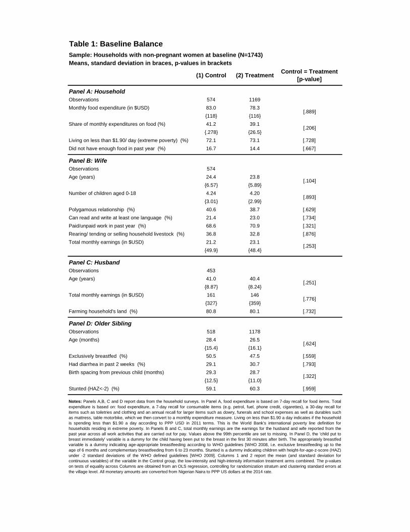
Table 1: Baseline Balance

Sample: Households with non-pregnant women at baseline (N=1743)

Means, standard deviation in braces, p-values in brackets

(1) Control (2) TreatmentControl = Treatment

[p-value]

Panel A: Household

Observations 574 1169

Monthly food expenditure (in $USD) 83.0 78.3

{118} {116}

Share of monthly expenditures on food (%) 41.2 39.1

{.278} {26.5}

Living on less than $1.90/ day (extreme poverty) (%) 72.1 73.1 [.728]

Did not have enough food in past year (%) 16.7 14.4 [.667]

Panel B: Wife

Observations 574

Age (years) 24.4 23.8

{6.57} {5.89}

Number of children aged 0-18 4.24 4.20

{3.01} {2.99}

Polygamous relationship (%) 40.6 38.7 [.629]

Can read and write at least one language (%) 21.4 23.0 [.734]

Paid/unpaid work in past year (%) 68.6 70.9 [.321]

Rearing/ tending or selling household livestock (%) 36.8 32.8 [.876]

Total monthly earnings (in $USD) 21.2 23.1

{49.9} {48.4}

Panel C: Husband

Observations 453

Age (years) 41.0 40.4

{8.87} {8.24}

Total monthly earnings (in $USD) 161 146

{327} {359}

Farming household's land (%) 80.8 80.1 [.732]

Panel D: Older Sibling

Observations 518 1178

Age (months) 28.4 26.5

{15.4} {16.1}

Exclusively breastfed (%) 50.5 47.5 [.559]

Had diarrhea in past 2 weeks (%) 29.1 30.7 [.793]

Birth spacing from previous child (months) 29.3 28.7

{12.5} {11.0}

Stunted (HAZ<-2) (%) 59.1 60.3 [.959]

Notes: Panels A,B, C and D report data from the household surveys. In Panel A, food expenditure is based on 7-day recall for food items. Total

expenditure is based on: food expenditure, a 7-day recall for consumable items (e.g. petrol, fuel, phone credit, cigarettes), a 30-day recall for

items such as toiletries and clothing and an annual recall for larger items such as dowry, funerals and school expenses as well as durables such

as mattress, table motorbike, which we then convert to a monthly expenditure measure. Living on less than $1.90 a day indicates if the household

is spending less than $1.90 a day according to PPP USD in 2011 terms. This is the World Bank's international poverty line definition for

households residing in extreme poverty. In Panels B and C, total monthly earnings are the earnings for the husband and wife reported from the

past year across all work activities that are carried out for pay. Values above the 99th percentile are set to missing. In Panel D, the 'child put to

breast immediately' variable is a dummy for the child having been put to the breast in the first 30 minutes after birth. The appropriately breastfed

variable is a dummy indicating age-appropriate breastfeeding according to WHO guidelines [WHO 2008, i.e. exclusive breastfeeding up to the

age of 6 months and complementary breastfeeding from 6 to 23 months. Stunted is a dummy indicating children with height-for-age-z-score (HAZ)

under -2 standard deviations of the WHO defined guidelines [WHO 2009]. Columns 1 and 2 report the mean (and standard deviation for

continuous variables) of the variable in the Control group, the low-intensity and high-intensity information treatment arms combined. The p-values

on tests of equality across Columns are obtained from an OLS regression, controlling for randomization stratum and clustering standard errors at

the village level. All monetary amounts are converted from Nigerian Naira to PPP US dollars at the 2014 rate.

[.889]

[.206]

[.104]

[.893]

[.253]

[.251]

[.776]

[.624]

[.322]

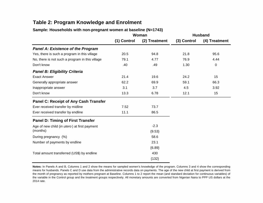
Table 2: Program Knowledge and Enrolment

Sample: Households with non-pregnant women at baseline (N=1743)

(1) Control (2) Treatment (3) Control (4) Treatment

Panel A: Existence of the Program

Yes, there is such a program in this village 20.5 94.8 21.8 95.6

No, there is not such a program in this village 79.1 4.77 76.9 4.44

Don't know .40 .49 1.30 0

Panel B: Eligibility Criteria

Exact Answer 21.4 19.6 24.2 15

Generally appropriate answer 62.2 69.9 59.1 66.3

Inappropriate answer 3.1 3.7 4.5 3.92

Don't know 13.3 6.78 12.1 15

Panel C: Receipt of Any Cash Transfer

Ever received transfer by midline 7.52 73.7

Ever received transfer by endline 11.1 86.5

Panel D: Timing of First Transfer

-2.3

{9.53}

During pregnancy (%) 58.6

Number of payments by endline 23.1

{6.89}

Total amount transferred (US$) by endline 430

{132}

Woman Husband

Notes: In Panels A and B, Columns 1 and 2 show the means for sampled women’s knowledge of the program. Columns 3 and 4 show the corresponding

means for husbands. Panels C and D use data from the administrative records data on payments. The age of the new child at first payment is derived fromthe month of pregnancy as reported by mothers pregnant at Baseline. Columns 1 to 2 report the mean (and standard deviation for continuous variables) ofthe variable in the Control group and the treatment groups respectively. All monetary amounts are converted from Nigerian Naira to PPP US dollars at the

2014 rate.

Age of new child (in utero ) at first payment(months)

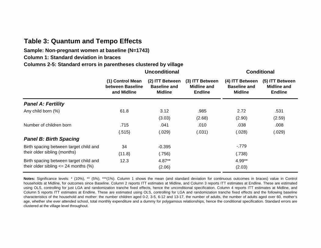
Table 3: Quantum and Tempo Effects

Sample: Non-pregnant women at baseline (N=1743)

Column 1: Standard deviation in braces

Columns 2-5: Standard errors in parentheses clustered by village

(1) Control Mean

between Baseline

and Midline

(2) ITT Between

Baseline and

Midline

(3) ITT Between

Midline and

Endline

(4) ITT Between

Baseline and

Midline

(5) ITT Between

Midline and

Endline

Any child born (%) 61.8 3.12 .985 2.72 .531

(3.03) (2.68) (2.90) (2.59)

Number of children born .715 .041 .010 .038 .008

{.515} (.029) (.031) (.028) (.029)

34 -0.395 -.779

{11.8} (.756) (.738)

12.3 4.87** 4.99**

(2.06) (2.03)

Notes: Significance levels: * (10%), ** (5%), ***(1%). Column 1 shows the mean (and standard deviation for continuous outcomes in braces) value in Controlhouseholds at Midline, for outcomes since Baseline. Column 2 reports ITT estimates at Midline, and Column 3 reports ITT estimates at Endline. These are estimatedusing OLS, controlling for just LGA and randomization tranche fixed effects, hence the unconditional specification. Column 4 reports ITT estimates at Midline, andColumn 5 reports ITT estimates at Endline. These are estimated using OLS, controlling for LGA and randomization tranche fixed effects and the following baselinecharacteristics of the household and mother: the number children aged 0-2, 3-5, 6-12 and 13-17, the number of adults, the number of adults aged over 60, mother’sage, whether she ever attended school, total monthly expenditure and a dummy for polygamous relationships, hence the conditional specification. Standard errors areclustered at the village level throughout.

Unconditional

Panel A: Fertility

Panel B: Birth Spacing

Conditional

Birth spacing between target child andtheir older sibling (months)

Birth spacing between target child andtheir older sibling <= 24 months (%)

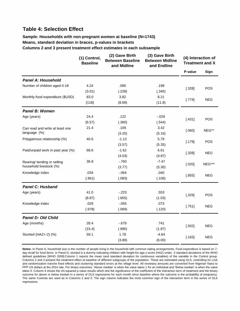
Table 4: Selection Effect

Sample: Households with non-pregnant women at baseline (N=1743)

Means, standard deviation in braces, p-values in brackets

Columns 2 and 3 present treatment effect estimates in each subsample

(1) Control,

Baseline

(2) Gave Birth

Between Baseline

and Midline

(3) Gave Birth

Between Midline

and Endline

P-value Sign

Panel A: Household

Number of children aged 0-18 4.24 .095 .199

{3.01} (.228) (.345)

Monthly food expenditure ($USD) 83.0 3.82 8.21

{118} (8.69) (11.8)

Panel B: Women

Age (years) 24.4 .122 -.029

{6.57} (.360) (.544)

21.4 .109 3.42

(3.20) (5.16)

Polygamous relationship (%) 40.6 -1.13 5.79

(3.57) (5.35)

Paid/unpaid work in past year (%) 68.6 -1.62 6.61

(4.03) (4.87)

36.8 -.760 -7.47

(3.77) (5.30)

Knowledge index .034 -.064 .040

{.961} (.083) (.106)

Panel C: Husband

Age (years) 41.0 -.223 .553

{8.87} (.655) (1.03)

Knowledge index .029 -.055 .073

{.978} (.069) (.120)

Panel D: Old Child

Age (months) 28.4 -.679 .741

{15.4} (.990) (1.87)

Stunted (HAZ<-2) (%) 59.1 1.78 -4.64

(3.89) (6.00)

NEG

POS

NEG

NEG

Notes: In Panel A, household size is the number of people living in the household with common eating arrangements. Food expenditure is based on 7-

day recall for food items. In Panel D, stunted is a dummy indicating children with height-for-age-z-score (HAZ) under -2 standard deviations of the WHOdefined guidelines [WHO 2009].Column 1 reports the mean (and standard deviation for continuous variables) of the variable in the Control group.Columns 2 and 3 present the treatment effect at baseline of different subgroups of the population. These are estimated using OLS, controlling for LGAand randomization tranche fixed effects and clustering standard errors at the village level. All monetary amounts are converted from Nigerian Naira toPPP US dollars at the 2014 rate. For binary outcomes, 'Above median' is when the value takes 1 for an individual and 'Below median' is when the valuetakes 0. Column 4 shows the chi-squared p-value results which test the significance of the coefficient of the interaction term of treatment and the binaryoutcome for above or below median in a series of OLS regressions for each month since baseline where the outcome is the probability of pregnancy.The same Controls are used as in Columns 2 and 3. The sign column indicates the most common sign of the interaction term in the series of OLSregressions.

[.751]

[.329]

NEG

[.163]

[.502]

NEG***

NEG

[.328] POS

[.431]

[.774]

POS

(4) Interaction of

Treatment and X

Rearing/ tending or sellinghousehold livestock (%)

[.020]

[.855]

NEG

Can read and write at least onelanguage (%)

[.328]

[.060]

[.179]

NEG**

POS

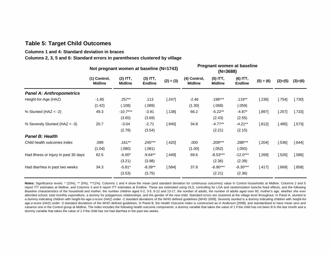
Table 5: Target Child Outcomes

Columns 1 and 4: Standard deviation in braces

Columns 2, 3, 5 and 6: Standard errors in parentheses clustered by village

(1) Control,

Midline

(2) ITT,

Midline

(3) ITT,

Endline(2) = (3)

(4) Control,

Midline

(5) ITT,

Midline

(6) ITT,

Endline(5) = (6) (2)=(5) (3)=(6)

Panel A: Anthropometrics

Height-for-Age (HAZ) -1.85 .257** .113 [.247] -2.46 .198*** .119** [.236] [.754] [.730]

{1.42} (.108) (.089) {1.30} (.068) (.059)

% Stunted (HAZ < -2) 49.3 -10.7*** -3.91 [.138] 66.2 -5.22** -4.87* [.897] [.257] [.733]

(3.65) (3.69) (2.43) (2.55)

% Severely Stunted (HAZ < -3) 20.7 -3.04 -2.71 [.940] 34.8 -4.77** -4.21** [.812] [.485] [.573]

(2.78) (3.54) (2.21) (2.15)

Panel B: Health

Child health outcomes index .099 .161** .245*** [.420] .000 .209*** .288*** [.204] [.536] [.644]

{1.04} (.080) (.081) {1.00} (.052) (.050)

Had illness or injury in past 30 days 62.6 -6.00* -9.64** [.449] 69.6 -8.53*** -12.0*** [.269] [.526] [.586]

(3.21) (3.98) (2.36) (2.39)

Had diarrhea in past two weeks 34.3 -5.81* -8.39** [.584] 37.8 -6.90*** -9.30*** [.417] [.669] [.858]

(3.53) (3.75) (2.21) (2.36)

Pregnant women at baseline

(N=3688)Not pregnant women at baseline (N=1743)

Notes: Significance levels: * (10%), ** (5%), ***(1%). Columns 1 and 4 show the mean (and standard deviation for continuous outcomes) value in Control households at Midline. Columns 2 and 5

report ITT estimates at Midline, and Columns 3 and 6 report ITT estimates at Endline. These are estimated using OLS, controlling for LGA and randomization tranche fixed effects, and the following

Baseline characteristics of the household and mother: the number children aged 0-2, 3-5, 6-12 and 13-17, the number of adults, the number of adults aged over 60, mother’s age, whether she ever

attended school, total monthly expenditure, a dummy for polygamous relationships, and the gender of the new child. Standard errors are clustered at the village level throughout. In Panel A, stunted is

a dummy indicating children with height-for-age-z-score (HAZ) under -2 standard deviations of the WHO defined guidelines [WHO 2009]. Severely stunted is a dummy indicating children with height-for-

age-z-score (HAZ) under -3 standard deviations of the WHO defined guidelines. In Panel B, the Health Outcome Index is constructed as in Anderson [2008], and standardized to have mean zero and

variance one in the Control group at Midline. The index includes the following health outcome components: a dummy variable that takes the value of 1 if the child has not been ill in the last month and a

dummy variable that takes the value of 1 if the child has not had diarrhea in the past two weeks.

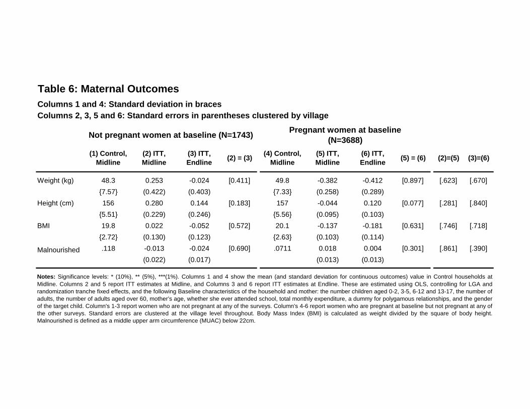
Table 6: Maternal Outcomes

Columns 1 and 4: Standard deviation in braces

Columns 2, 3, 5 and 6: Standard errors in parentheses clustered by village

(1) Control,

Midline

(2) ITT,

Midline

(3) ITT,

Endline(2) = (3)

(4) Control,

Midline

(5) ITT,

Midline

(6) ITT,

Endline(5) = (6) (2)=(5) (3)=(6)

Weight (kg) 48.3 0.253 -0.024 [0.411] 49.8 -0.382 -0.412 [0.897] [.623] [.670]

{7.57} (0.422) (0.403) {7.33} (0.258) (0.289)

Height (cm) 156 0.280 0.144 [0.183] 157 -0.044 0.120 [0.077] [.281] [.840]

{5.51} (0.229) (0.246) {5.56} (0.095) (0.103)

BMI 19.8 0.022 -0.052 [0.572] 20.1 -0.137 -0.181 [0.631] [.746] [.718]

{2.72} (0.130) (0.123) {2.63} (0.103) (0.114)

Malnourished .118 -0.013 -0.024 [0.690] .0711 0.018 0.004 [0.301] [.861] [.390]

(0.022) (0.017) (0.013) (0.013)

Not pregnant women at baseline (N=1743)Pregnant women at baseline

(N=3688)

Notes: Significance levels: * (10%), ** (5%), ***(1%). Columns 1 and 4 show the mean (and standard deviation for continuous outcomes) value in Control households at

Midline. Columns 2 and 5 report ITT estimates at Midline, and Columns 3 and 6 report ITT estimates at Endline. These are estimated using OLS, controlling for LGA andrandomization tranche fixed effects, and the following Baseline characteristics of the household and mother: the number children aged 0-2, 3-5, 6-12 and 13-17, the number ofadults, the number of adults aged over 60, mother’s age, whether she ever attended school, total monthly expenditure, a dummy for polygamous relationships, and the genderof the target child. Column's 1-3 report women who are not pregnant at any of the surveys. Column's 4-6 report women who are pregnant at baseline but not pregnant at any ofthe other surveys. Standard errors are clustered at the village level throughout. Body Mass Index (BMI) is calculated as weight divided by the square of body height.Malnourished is defined as a middle upper arm circumference (MUAC) below 22cm.

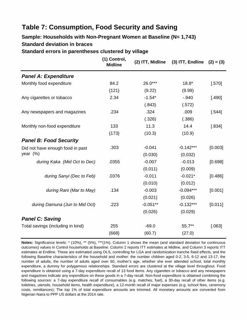
Standard deviation in braces

Standard errors in parentheses clustered by village

(1) Control,

Midline(2) ITT, Midline (3) ITT, Endline (2) = (3)

Panel A: Expenditure

Monthly food expenditure 84.2 26.0*** 18.8* [.570]

{121} (9.22) (9.99)

Any cigarettes or tobacco 2.34 -1.54* -.940 [.490]

(.843) (.572)

Any newspapers and magazines .234 .324 .009 [.544]

(.326) (.386)

Monthly non-food expenditure 133 11.3 14.4 [.834]

{173} (10.3) (10.9)

Panel B: Food Security

.303 -0.041 -0.142*** [0.003]

(0.030) (0.032)

during Kaka (Mid Oct to Dec) .0355 -0.007 -0.013 [0.698]

(0.011) (0.009)

during Sanyi (Dec to Feb) .0376 -0.011 -0.021* [0.486]

(0.010) (0.012)

during Rani (Mar to May) .134 -0.003 -0.094*** [0.001]

(0.021) (0.026)

during Damuna (Jun to Mid Oct) .223 -0.051** -0.132*** [0.011]

(0.026) (0.029)

Panel C: Saving

Total savings (including in kind) 255 -69.0 55.7** [.063]

{668} (60.7) (27.0)

Table 7: Consumption, Food Security and Saving

Sample: Households with Non-Pregnant Women at Baseline (N= 1,743)

Notes: Significance levels: * (10%), ** (5%), ***(1%). Column 1 shows the mean (and standard deviation for continuous

outcomes) values in Control households at Baseline. Column 2 reports ITT estimates at Midline, and Column 3 reports ITT

estimates at Endline. These are estimated using OLS, controlling for LGA and randomization tranche fixed effects, and the

following Baseline characteristics of the household and mother: the number children aged 0-2, 3-5, 6-12 and 13-17, the

number of adults, the number of adults aged over 60, mother’s age, whether she ever attended school, total monthly

expenditure, a dummy for polygamous relationships. Standard errors are clustered at the village level throughout. Food

expenditure is obtained using a 7-day expenditure recall of 13 food items. Any cigarettes or tobacco and any newspapers

and magazines indicate any expenditure on these goods in a 7-day recall. Non-food expenditure is obtained combining the

following sources: a 7-day expenditure recall of consumables (e.g. matches, fuel), a 30-day recall of other items (e.g.

toiletries, utensils, household items, health expenditure), a 12-month recall of major expenses (e.g. school fees, ceremony

costs, remittances); The top 1% of total expenditure amounts are trimmed. All monetary amounts are converted from

Nigerian Naira to PPP US dollars at the 2014 rate.

Did not have enough food in pastyear (%)

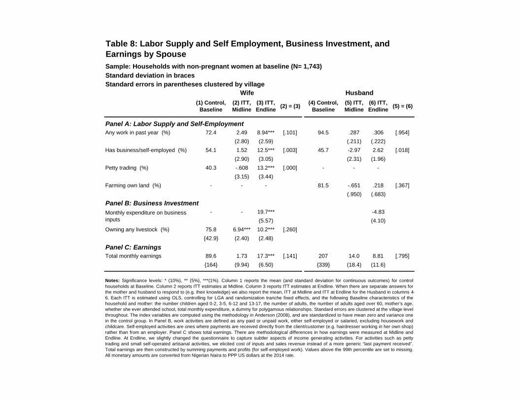
Standard deviation in braces

Standard errors in parentheses clustered by village

(1) Control,Baseline

(2) ITT,Midline

(3) ITT,Endline

(2) = (3)(4) Control,

Baseline(5) ITT,Midline

(6) ITT,Endline

(5) = (6)

Panel A: Labor Supply and Self-Employment

Any work in past year (%) 72.4 2.49 8.94*** [.101] 94.5 .287 .306 [.954]

(2.80) (2.59) (.211) (.222)

Has business/self-employed (%) 54.1 1.52 12.5*** [.003] 45.7 -2.97 2.62 [.018]

(2.90) (3.05) (2.31) (1.96)

Petty trading (%) 40.3 -.608 13.2*** [.000] - - -

(3.15) (3.44)

Farming own land (%) - - - 81.5 -.651 .218 [.367]

(.950) (.683)

Panel B: Business Investment

- - 19.7*** -4.83

(5.57) (4.10)

Owning any livestock (%) 75.8 6.94*** 10.2*** [.260]

{42.9} (2.40) (2.48)

Panel C: Earnings

Total monthly earnings 89.6 1.73 17.3*** [.141] 207 14.0 8.81 [.795]

{164} (9.94) (6.50) {339} (18.4) (11.6)

Table 8: Labor Supply and Self Employment, Business Investment, andEarnings by Spouse

Sample: Households with non-pregnant women at baseline (N= 1,743)

Wife Husband

Notes: Significance levels: * (10%), ** (5%), ***(1%). Column 1 reports the mean (and standard deviation for continuous outcomes) for control

households at Baseline. Column 2 reports ITT estimates at Midline. Column 3 reports ITT estimates at Endline. When there are separate answers forthe mother and husband to respond to (e.g. their knowledge) we also report the mean, ITT at Midline and ITT at Endline for the Husband in columns 4-6. Each ITT is estimated using OLS, controlling for LGA and randomization tranche fixed effects, and the following Baseline characteristics of thehousehold and mother: the number children aged 0-2, 3-5, 6-12 and 13-17, the number of adults, the number of adults aged over 60, mother’s age,whether she ever attended school, total monthly expenditure, a dummy for polygamous relationships. Standard errors are clustered at the village levelthroughout. The index variables are computed using the methodology in Anderson (2008), and are standardized to have mean zero and variance onein the control group. In Panel B, work activities are defined as any paid or unpaid work, either self-employed or salaried, excluding housework andchildcare. Self-employed activities are ones where payments are received directly from the client/customer (e.g. hairdresser working in her own shop)rather than from an employer. Panel C shows total earnings. There are methodological differences in how earnings were measured at Midline andEndline. At Endline, we slightly changed the questionnaire to capture subtler aspects of income generating activities. For activities such as pettytrading and small self-operated artisanal activities, we elicited cost of inputs and sales revenue instead of a more generic “last payment received”.Total earnings are then constructed by summing payments and profits (for self-employed work). Values above the 99th percentile are set to missing.All monetary amounts are converted from Nigerian Naira to PPP US dollars at the 2014 rate.

Monthly expenditure on businessinputs

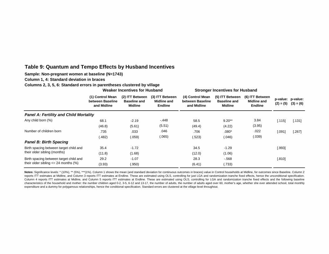
Table 9: Quantum and Tempo Effects by Husband Incentives

Sample: Non-pregnant women at baseline (N=1743)

Column 1, 4: Standard deviation in braces

Columns 2, 3, 5, 6: Standard errors in parentheses clustered by village

(1) Control Mean

between Baseline

and Midline

(2) ITT Between

Baseline and

Midline

(3) ITT Between

Midline and

Endline

(4) Control Mean

between Baseline

and Midline

(5) ITT Between

Baseline and

Midline

(6) ITT Between

Midline and

Endline

p-value:

(2) = (5)

p-value:

(3) = (6)

Any child born (%) 68.1 -2.19 -.448 58.5 9.20** 3.84 [.115] [.131]

(46.8) (5.61) (5.51) (49.4) (4.22) (3.95)

Number of children born .735 .033 .046 .706 .080* .022 [.091] [.267]

(.482) (.059) (.065) (.523) (.046) (.039)

Panel B: Birth Spacing

35.4 -1.72 34.5 -1.29 [.993]

(11.8) (1.68) (12.0) (1.06)

29.2 -1.07 28.3 -.568 [.810]

(3.93) (.950) (6.41) (.733)

Notes: Significance levels: * (10%), ** (5%), ***(1%). Column 1 shows the mean (and standard deviation for continuous outcomes in braces) value in Control households at Midline, for outcomes since Baseline. Column 2

reports ITT estimates at Midline, and Column 3 reports ITT estimates at Endline. These are estimated using OLS, controlling for just LGA and randomization tranche fixed effects, hence the unconditional specification.

Column 4 reports ITT estimates at Midline, and Column 5 reports ITT estimates at Endline. These are estimated using OLS, controlling for LGA and randomization tranche fixed effects and the following baseline

characteristics of the household and mother: the number children aged 0-2, 3-5, 6-12 and 13-17, the number of adults, the number of adults aged over 60, mother’s age, whether she ever attended school, total monthly

expenditure and a dummy for polygamous relationships, hence the conditional specification. Standard errors are clustered at the village level throughout.

Stronger Incentives for HusbandWeaker Incentives for Husband

Panel A: Fertility and Child Mortality

Birth spacing between target child andtheir older sibling (months)

Birth spacing between target child andtheir older sibling <= 24 months (%)

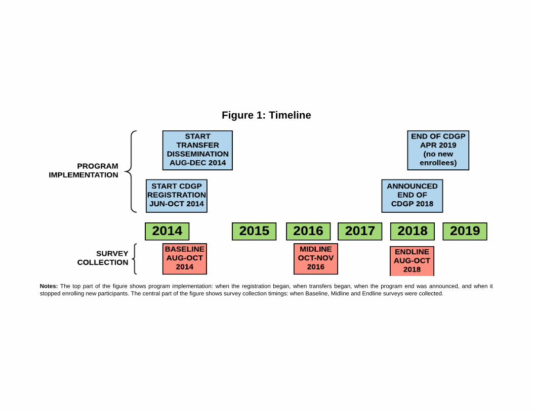
Notes: The top part of the figure shows program implementation: when the registration began, when transfers began, when the program end was announced, and when it

stopped enrolling new participants. The central part of the figure shows survey collection timings: when Baseline, Midline and Endline surveys were collected.

Figure 1: Timeline

Note: The number of women at risk are the number who have not become pregnant at the given months since baseline. They grey shaded area

shows any individual time period that is significantly different between treatment and control group (at the 5% significance level). The Chi-squared

statistic is estimated by running probit regressions of a dummy of pregnancy in each month on treatment. In these regressions we control for LGA

and randomization tranche fixed effects, and the following baseline characteristics of the household and mother: the number children aged 0-2, 3-5,

6-12 and 13-17, the number of adults, the number of adults aged over 60, mother’s age, whether she ever attended school, total monthly expenditure

and a dummy for polygamous relationship. The standard errors are clustered at the village level. The p-value reported comes testing the

significance on the treatment coefficient in each regression and testing with a Chi-squared statistic with 46 degrees of freedom.

Figure 2: Survival Probability of Not Becoming Pregnant

A. Unconditional Survival Probability

B. Adjusted at the Median for Base Covariates

Chi-squared = 62.5p-value = .053

Chi-squared = 68.0p-value = .019

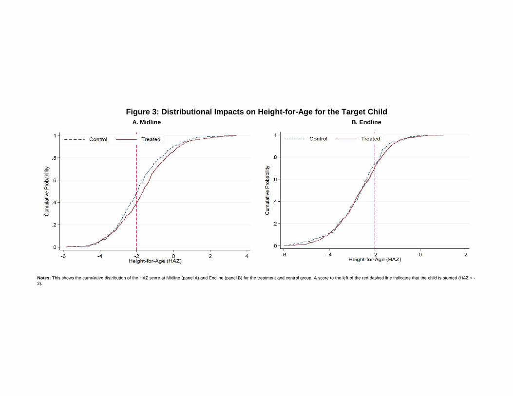
Notes: This shows the cumulative distribution of the HAZ score at Midline (panel A) and Endline (panel B) for the treatment and control group. A score to the left of the red dashed line indicates that the child is stunted (HAZ < -

2).

Figure 3: Distributional Impacts on Height-for-Age for the Target Child

A. Midline B. Endline

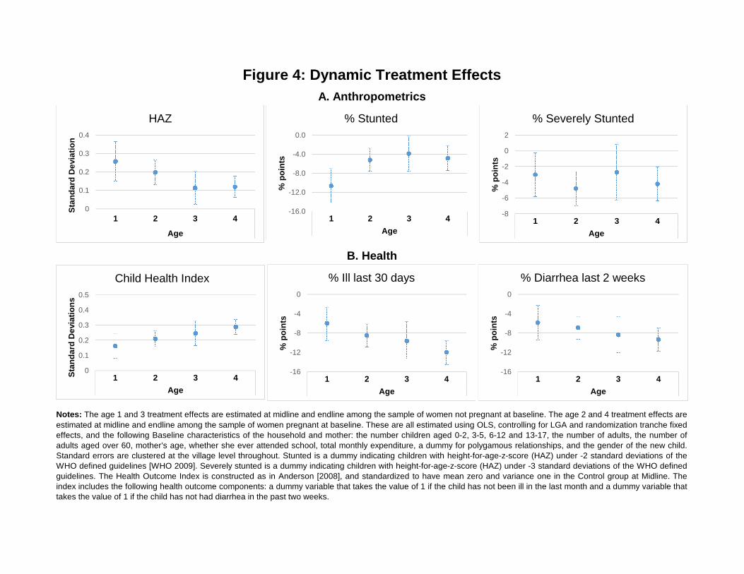
1 2 3 4

HAZ 0.257 0.198 0.113 0.119

SE (.108) (.068) (.089) (.059)

% Stunted -10.7 -5.22 -3.91 -4.87

(3.650) (2.430) (3.69) (2.550)

% Severely stunted-3.04 -4.77 -2.71 -4.21

2.78 2.21 3.54 2.15

Child health index0.161 0.209 0.245 0.288

0.08 0.052 0.08 0.05

Illness past 30 days -6 -8.53 -9.64 -12

3.21 2.36 3.98 2.39

Diarrhea past two weeks-5.81 -6.9 -8.39 -9.3

3.53 2.21 3.75 2.36

Notes: The age 1 and 3 treatment effects are estimated at midline and endline among the sample of women not pregnant at baseline. The age 2 and 4 treatment effects are

estimated at midline and endline among the sample of women pregnant at baseline. These are all estimated using OLS, controlling for LGA and randomization tranche fixedeffects, and the following Baseline characteristics of the household and mother: the number children aged 0-2, 3-5, 6-12 and 13-17, the number of adults, the number ofadults aged over 60, mother’s age, whether she ever attended school, total monthly expenditure, a dummy for polygamous relationships, and the gender of the new child.Standard errors are clustered at the village level throughout. Stunted is a dummy indicating children with height-for-age-z-score (HAZ) under -2 standard deviations of theWHO defined guidelines [WHO 2009]. Severely stunted is a dummy indicating children with height-for-age-z-score (HAZ) under -3 standard deviations of the WHO definedguidelines. The Health Outcome Index is constructed as in Anderson [2008], and standardized to have mean zero and variance one in the Control group at Midline. Theindex includes the following health outcome components: a dummy variable that takes the value of 1 if the child has not been ill in the last month and a dummy variable thattakes the value of 1 if the child has not had diarrhea in the past two weeks.

Age

Figure 4: Dynamic Treatment Effects

A. Anthropometrics

B. Health

0

0.1

0.2

0.3

0.4

1 2 3 4

Age

Sta

nd

ard

De

via

tio

n

HAZ

-16.0

-12.0

-8.0

-4.0

0.0

1 2 3 4

Age

%p

oin

ts

% Stunted

-8

-6

-4

-2

0

2

1 2 3 4

Age

%p

oin

ts

% Severely Stunted

0

0.1

0.2

0.3

0.4

0.5

1 2 3 4

Age

Sta

nd

ard

De

via

tio

ns

Child Health Index

-16

-12

-8

-4

0

1 2 3 4

Age

%p

oin

ts% Ill last 30 days

-16

-12

-8

-4

0

1 2 3 4

Age

%p

oin

ts

% Diarrhea last 2 weeks

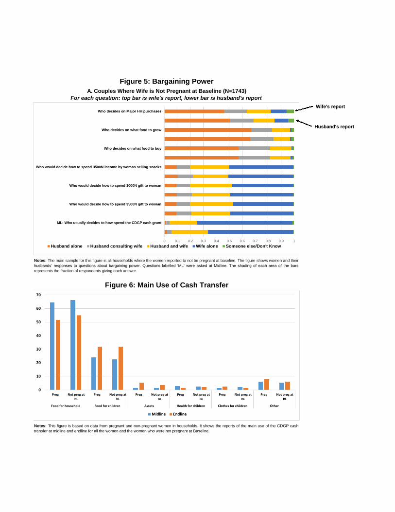
person Husband aloneHusband consulting womanHusband and woman jointlyWoman herselfSomeone else/Don't Know

Wom 0.462378 0.174612 0.183802 0.123492 0.055715

Husb 0.503729 0.187034 0.159495 0.10327 0.046472

Wom 0.672404 0.160643 0.138267 0.010327 0.018359

Husb 0.663798 0.180149 0.127367 0.011474 0.017212

Wom 0.571182 0.24438 0.165418 0.008646 0.010375

Husb 0.574297 0.243259 0.155479 0.014343 0.012622

Wom 0.095812 0.102123 0.301779 0.493402 0.006885

Husb 0.104418 0.114171 0.274814 0.501434 0.005164

Wom 0.093517 0.104991 0.324154 0.475043 0.002295

Husb 0.096386 0.115892 0.291452 0.491107 0.005164

Wom 0.092369 0.106139 0.33276 0.466437 0.002295

Husb 0.093517 0.115318 0.299484 0.487665 0.004016

Wom 0.014192 0.025109 0.210699 0.737991 0.012009

Husb 0.019084 0.03626 0.280534 0.656489 0.007633

Midline Endline

Food for householdPreg 64.5 51.5

Not preg at BL 66.3 55

Food for childrenPreg 23.8 31.7

Not preg at BL 22.5 31.8

Assets Preg 1.5 5.4

Not preg at BL 1.5 3.5

Health for childrenPreg 2.7 1.4

Not preg at BL 2.4 2.2

Clothes for childrenPreg 1.4 2.3

Not preg at BL 2.1 1.4

Other Preg 6.1 7.7

Not preg at BL 5.2 6.1

Figure 5: Bargaining Power

A. Couples Where Wife is Not Pregnant at Baseline (N=1743)

Notes: The main sample for this figure is all households where the women reported to not be pregnant at baseline. The figure shows women and their

husbands' responses to questions about bargaining power. Questions labelled 'ML' were asked at Midline. The shading of each area of the bars

represents the fraction of respondents giving each answer.

Figure 6: Main Use of Cash Transfer

For each question: top bar is wife's report, lower bar is husband's report

Notes: This figure is based on data from pregnant and non-pregnant women in households. It shows the reports of the main use of the CDGP cash

transfer at midline and endline for all the women and the women who were not pregnant at Baseline.

Who

decides

ML: Who

usually

Who

would

Who

would

Who

would

Who

decides

Who

decides

0 0.1 0.2 0.3 0.4 0.5 0.6 0.7 0.8 0.9 1

Who decides on Major HH purchases

Who decides on what food to grow

Who decides on what food to buy

Who would decide how to spend 3500N income by woman selling snacks

Who would decide how to spend 1000N gift to woman

Who would decide how to spend 3500N gift to woman

ML: Who usually decides to how spend the CDGP cash grant

Husband alone Husband consulting wife Husband and wife Wife alone Someone else/Don't Know

0

10

20

30

40

50

60

70

Preg Not preg atBL

Preg Not preg atBL

Preg Not preg atBL

Preg Not preg atBL

Preg Not preg atBL

Preg Not preg atBL

Food for household Food for children Assets Health for children Clothes for children Other

Midline Endline

Husband's report

Wife's report

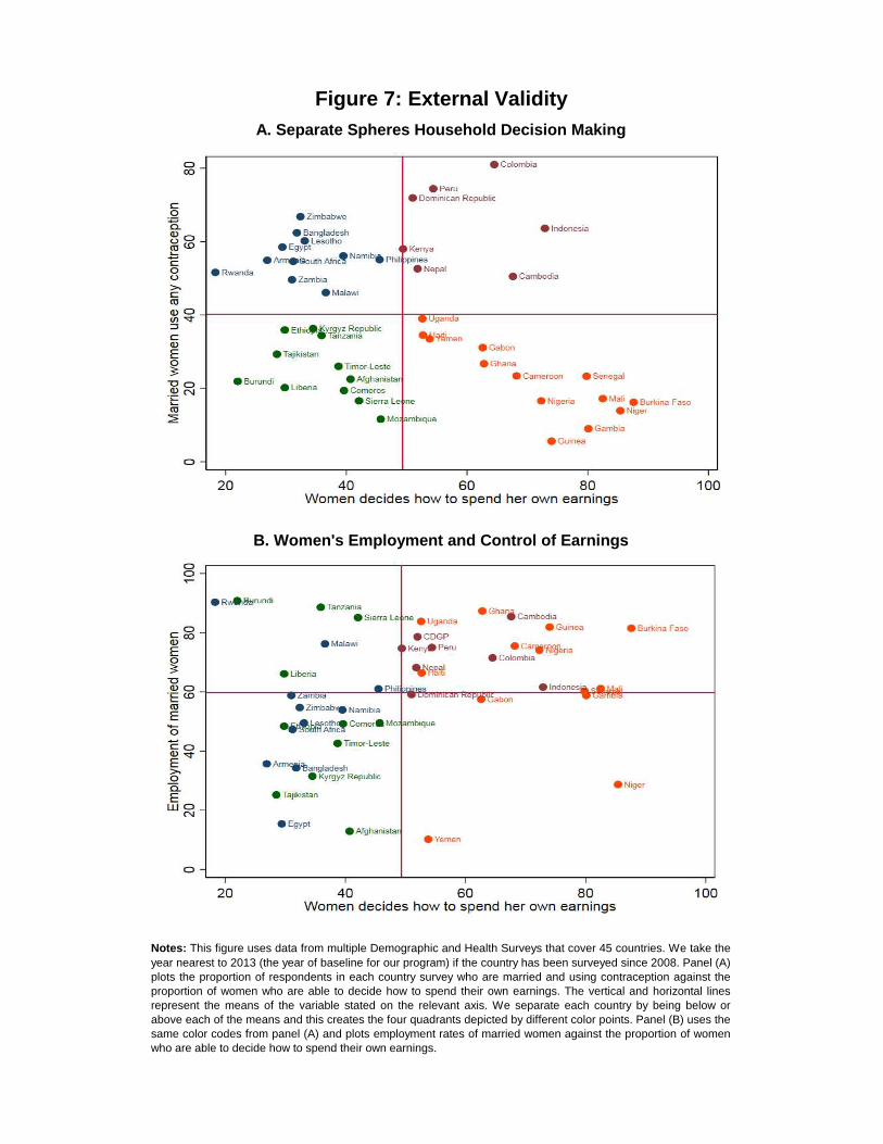
A. Separate Spheres Household Decision Making

Figure 7: External Validity

B. Women's Employment and Control of Earnings

Notes: This figure uses data from multiple Demographic and Health Surveys that cover 45 countries. We take the

year nearest to 2013 (the year of baseline for our program) if the country has been surveyed since 2008. Panel (A)plots the proportion of respondents in each country survey who are married and using contraception against theproportion of women who are able to decide how to spend their own earnings. The vertical and horizontal linesrepresent the means of the variable stated on the relevant axis. We separate each country by being below orabove each of the means and this creates the four quadrants depicted by different color points. Panel (B) uses thesame color codes from panel (A) and plots employment rates of married women against the proportion of womenwho are able to decide how to spend their own earnings.

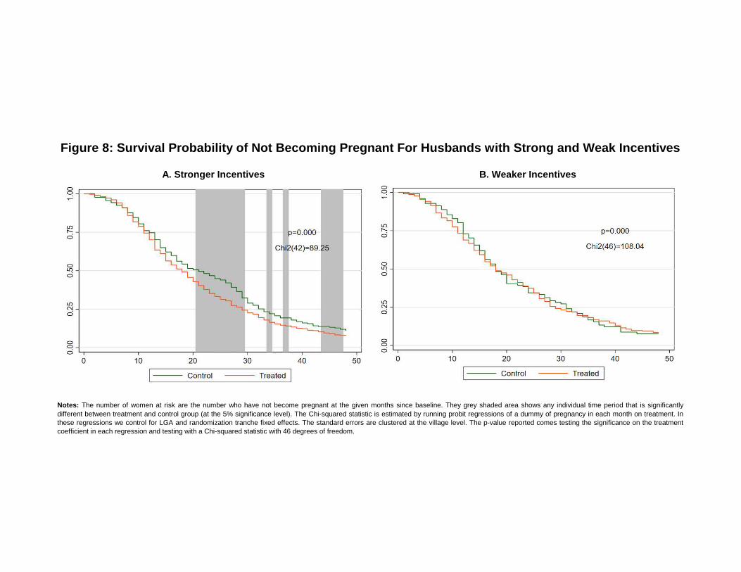
Notes: The number of women at risk are the number who have not become pregnant at the given months since baseline. They grey shaded area shows any individual time period that is significantly

different between treatment and control group (at the 5% significance level). The Chi-squared statistic is estimated by running probit regressions of a dummy of pregnancy in each month on treatment. Inthese regressions we control for LGA and randomization tranche fixed effects. The standard errors are clustered at the village level. The p-value reported comes testing the significance on the treatmentcoefficient in each regression and testing with a Chi-squared statistic with 46 degrees of freedom.

Figure 8: Survival Probability of Not Becoming Pregnant For Husbands with Strong and Weak Incentives

A. Stronger Incentives B. Weaker Incentives

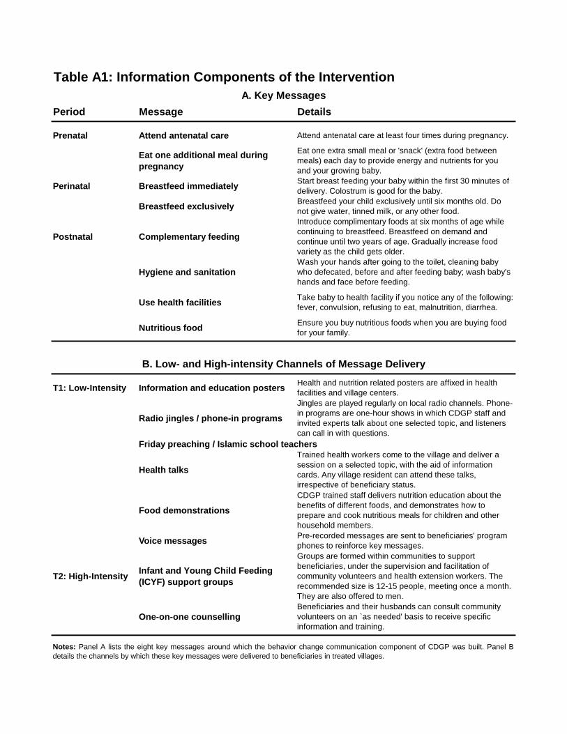
Table A1: Information Components of the Intervention

Period Message Details

Prenatal Attend antenatal care Attend antenatal care at least four times during pregnancy.

Eat one additional meal during

pregnancy

Eat one extra small meal or 'snack' (extra food betweenmeals) each day to provide energy and nutrients for youand your growing baby.

Perinatal Breastfeed immediatelyStart breast feeding your baby within the first 30 minutes ofdelivery. Colostrum is good for the baby.

Breastfeed exclusivelyBreastfeed your child exclusively until six months old. Donot give water, tinned milk, or any other food.

Postnatal Complementary feeding

Introduce complimentary foods at six months of age whilecontinuing to breastfeed. Breastfeed on demand andcontinue until two years of age. Gradually increase foodvariety as the child gets older.

Hygiene and sanitationWash your hands after going to the toilet, cleaning babywho defecated, before and after feeding baby; wash baby'shands and face before feeding.

Use health facilitiesTake baby to health facility if you notice any of the following:fever, convulsion, refusing to eat, malnutrition, diarrhea.

Nutritious foodEnsure you buy nutritious foods when you are buying foodfor your family.

T1: Low-Intensity Information and education postersHealth and nutrition related posters are affixed in healthfacilities and village centers.

Radio jingles / phone-in programs

Jingles are played regularly on local radio channels. Phone-in programs are one-hour shows in which CDGP staff andinvited experts talk about one selected topic, and listenerscan call in with questions.

Friday preaching / Islamic school teachers

Health talks

Trained health workers come to the village and deliver asession on a selected topic, with the aid of informationcards. Any village resident can attend these talks,irrespective of beneficiary status.

Food demonstrations

CDGP trained staff delivers nutrition education about thebenefits of different foods, and demonstrates how toprepare and cook nutritious meals for children and otherhousehold members.

Voice messagesPre-recorded messages are sent to beneficiaries' programphones to reinforce key messages.

T2: High-IntensityInfant and Young Child Feeding

(ICYF) support groups

Groups are formed within communities to supportbeneficiaries, under the supervision and facilitation ofcommunity volunteers and health extension workers. Therecommended size is 12-15 people, meeting once a month.They are also offered to men.

One-on-one counsellingBeneficiaries and their husbands can consult communityvolunteers on an `as needed' basis to receive specificinformation and training.

A. Key Messages

B. Low- and High-intensity Channels of Message Delivery

Notes: Panel A lists the eight key messages around which the behavior change communication component of CDGP was built. Panel B

details the channels by which these key messages were delivered to beneficiaries in treated villages. 

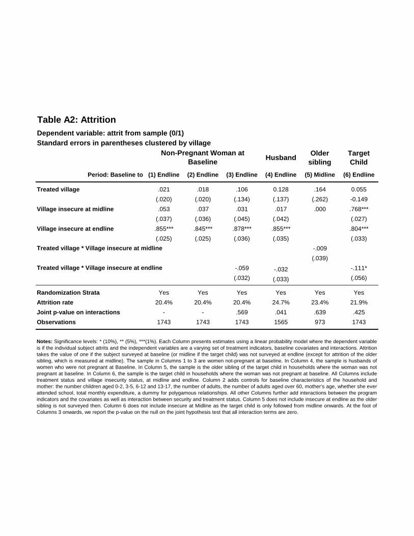
Table A2: Attrition

Dependent variable: attrit from sample (0/1)

Standard errors in parentheses clustered by village

HusbandOlder

sibling

Target

Child

Period: Baseline to (1) Endline (2) Endline (3) Endline (4) Endline (5) Midline (6) Endline

Treated village .021 .018 .106 0.128 .164 0.055

(.020) (.020) (.134) (.137) (.262) -0.149

Village insecure at midline .053 .037 .031 .017 .000 .768***

(.037) (.036) (.045) (.042) (.027)

Village insecure at endline .855*** .845*** .878*** .855*** .804***

(.025) (.025) (.036) (.035) (.033)

-.009

(.039)

-.059 -.032 -.111*

(.032) (.033) (.056)

Randomization Strata Yes Yes Yes Yes Yes Yes

Attrition rate 20.4% 20.4% 20.4% 24.7% 23.4% 21.9%

Joint p-value on interactions - - .569 .041 .639 .425

Observations 1743 1743 1743 1565 973 1743

Notes: Significance levels: * (10%), ** (5%), ***(1%). Each Column presents estimates using a linear probability model where the dependent variable

is if the individual subject attrits and the independent variables are a varying set of treatment indicators, baseline covariates and interactions. Attrition

takes the value of one if the subject surveyed at baseline (or midline if the target child) was not surveyed at endline (except for attrition of the older

sibling, which is measured at midline). The sample in Columns 1 to 3 are women not-pregnant at baseline. In Column 4, the sample is husbands of

women who were not pregnant at Baseline. In Column 5, the sample is the older sibling of the target child in households where the woman was not

pregnant at baseline. In Column 6, the sample is the target child in households where the woman was not pregnant at baseline. All Columns include

treatment status and village insecurity status, at midline and endline. Column 2 adds controls for baseline characteristics of the household and

mother: the number children aged 0-2, 3-5, 6-12 and 13-17, the number of adults, the number of adults aged over 60, mother’s age, whether she ever

attended school, total monthly expenditure, a dummy for polygamous relationships. All other Columns further add interactions between the program

indicators and the covariates as well as interaction between security and treatment status. Column 5 does not include insecure at endline as the older

sibling is not surveyed then. Column 6 does not include insecure at Midline as the target child is only followed from midline onwards. At the foot of

Columns 3 onwards, we report the p-value on the null on the joint hypothesis test that all interaction terms are zero.

Non-Pregnant Woman at

Baseline

Treated village * Village insecure at midline

Treated village * Village insecure at endline

Table A3: Fertility Results, Alternative Weighting

Sample: Non-pregnant women at baseline (N=1743)

Columns 1, 4: Standard deviation in braces

Columns 2, 3, 5, 6, 7 and 8: Standard errors in parentheses clustered by village

(1) Control

Mean

(2) ITT

Between

Baseline and

Midline

(3) ITT

Between

Midline and

Endline

(4) Control

Mean

(5) ITT

Between

Baseline and

Midline

(6) ITT

Between

Midline and

Endline

(7) ITT

Between

Baseline and

Midline

(8) ITT

Between

Midline and

Endline

Any child born (%) 79.8 4.33 1.01 79.9 3.86 .734 1.207 .378

(3.02) (2.72) (2.98) 2.662 (2.85) (2.64)

Number of children born .984 .047 .006 .976 .042 .005 .027 .007

(.031) (.031) (.030) (.030) (.027) (.030)

34.2 -.868 34 -.779 34.7

(.737) (.729)

11.8 4.52** 14.4 4.58** 10.8

(2.01) (1.93)

Weights: LPMWeights: ProbitWeights: LPM, Below

Median

Notes: Significance levels: * (10%), ** (5%), ***(1%). We reweight the sample based on their probability of becoming pregnant in two ways. The likelihood of becoming pregnant was established using

a prediction model based on data from the 2013 Nigeria Demographic and Health Survey (NPC and ICF, 2014). The probability of giving birth in the next two years was modelled as a function of

woman’s age, time since last birth, household size, number of children aged under and over 5 years in household, and TV ownership. The estimated coefficients from a linear probability model on the

DHS data were then used to predict pregnancy probability in the CDGP listing data, the Probit weights are used in column 1 (the weighted control mean), 2 and 3 and the LPM weights are used in

column 4 (weighted control mean), 5 and 6. Column 2 and 5 reports ITT estimates at Midline, and Column 3 and 6 reports ITT estimates at Endline. Column 7 and 8 restrict the sample to those who

have below median probability of becoming pregnant. All ITT impacts are estimated using OLS, controlling for LGA and randomization tranche fixed effects, and the following Baseline characteristics

of the household and mother: the number children aged 0-2, 3-5, 6-12 and 13-17, the number of adults, the number of adults aged over 60, mother’s age, whether she ever attended school, total

monthly expenditure and a dummy for polygamous relationships. In Panel B we also control for the month in utero of the new child. Standard errors are clustered at the village level throughout. Any

child born refers to a child born between Baseline and Midline (Midline and Endline) in Column 2 (3). The age child death outcomes relate to children born between Baseline and Midline.

Birth spacing between target child andtheir older sibling (months)

Birth spacing between target child andtheir older sibling <= 24 months (%)

Panel A: Fertility

Panel B: Birth Spacing

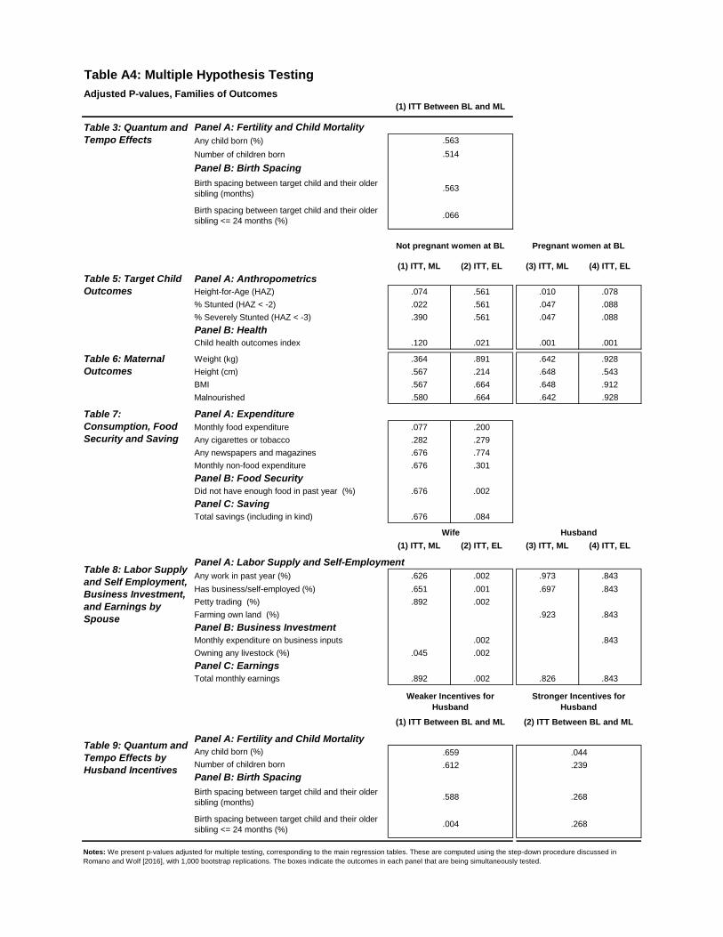
Table A4: Multiple Hypothesis Testing

Adjusted P-values, Families of Outcomes

Panel A: Fertility and Child Mortality

Any child born (%)

Number of children born

Panel B: Birth Spacing

Birth spacing between target child and their oldersibling (months)

Birth spacing between target child and their oldersibling <= 24 months (%)

(1) ITT, ML (2) ITT, EL (3) ITT, ML (4) ITT, EL

Panel A: AnthropometricsHeight-for-Age (HAZ) .074 .561 .010 .078

% Stunted (HAZ < -2) .022 .561 .047 .088

% Severely Stunted (HAZ < -3) .390 .561 .047 .088

Panel B: HealthChild health outcomes index .120 .021 .001 .001

Weight (kg) .364 .891 .642 .928

Height (cm) .567 .214 .648 .543

BMI .567 .664 .648 .912

Malnourished .580 .664 .642 .928

Panel A: Expenditure

Monthly food expenditure .077 .200

Any cigarettes or tobacco .282 .279

Any newspapers and magazines .676 .774

Monthly non-food expenditure .676 .301

Panel B: Food SecurityDid not have enough food in past year (%) .676 .002

Panel C: SavingTotal savings (including in kind) .676 .084

(1) ITT, ML (2) ITT, EL (3) ITT, ML (4) ITT, EL

Panel A: Labor Supply and Self-Employment

Any work in past year (%) .626 .002 .973 .843

Has business/self-employed (%) .651 .001 .697 .843

Petty trading (%) .892 .002

Farming own land (%) .923 .843

Panel B: Business InvestmentMonthly expenditure on business inputs .002 .843

Owning any livestock (%) .045 .002

Panel C: EarningsTotal monthly earnings .892 .002 .826 .843

Panel A: Fertility and Child MortalityAny child born (%)

Number of children born

Panel B: Birth Spacing

Birth spacing between target child and their oldersibling (months)

Birth spacing between target child and their oldersibling <= 24 months (%)

.239

.044

.588

Table 5: Target ChildOutcomes

Table 6: MaternalOutcomes

Table 7:Consumption, FoodSecurity and Saving

Table 8: Labor Supplyand Self Employment,Business Investment,and Earnings bySpouse

Table 9: Quantum andTempo Effects byHusband Incentives

(1) ITT Between BL and ML (2) ITT Between BL and ML

.659

.612

.004

Weaker Incentives for

Husband

Stronger Incentives for

Husband

Notes: We present p-values adjusted for multiple testing, corresponding to the main regression tables. These are computed using the step-down procedure discussed in

Romano and Wolf [2016], with 1,000 bootstrap replications. The boxes indicate the outcomes in each panel that are being simultaneously tested.

(1) ITT Between BL and ML

.563

.514

.563

.066

Table 3: Quantum andTempo Effects

Not pregnant women at BL Pregnant women at BL

Wife Husband

.268

.268

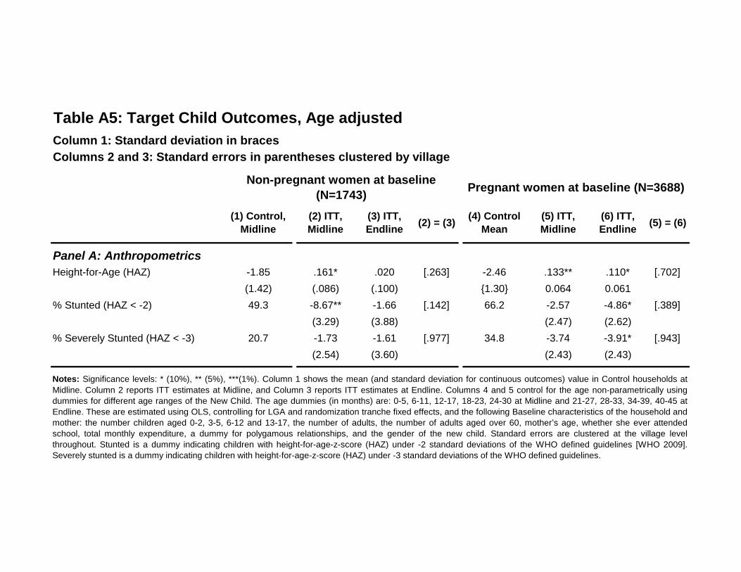
Table A5: Target Child Outcomes, Age adjusted

Column 1: Standard deviation in braces

Columns 2 and 3: Standard errors in parentheses clustered by village

(1) Control,

Midline

(2) ITT,

Midline

(3) ITT,

Endline(2) = (3)

(4) Control

Mean

(5) ITT,

Midline

(6) ITT,

Endline(5) = (6)

Panel A: Anthropometrics

Height-for-Age (HAZ) -1.85 .161* .020 [.263] -2.46 .133** .110* [.702]

(1.42) (.086) (.100) {1.30} 0.064 0.061

% Stunted (HAZ < -2) 49.3 -8.67** -1.66 [.142] 66.2 -2.57 -4.86* [.389]

(3.29) (3.88) (2.47) (2.62)

% Severely Stunted (HAZ < -3) 20.7 -1.73 -1.61 [.977] 34.8 -3.74 -3.91* [.943]

(2.54) (3.60) (2.43) (2.43)

Pregnant women at baseline (N=3688)Non-pregnant women at baseline

(N=1743)

Notes: Significance levels: * (10%), ** (5%), ***(1%). Column 1 shows the mean (and standard deviation for continuous outcomes) value in Control households at

Midline. Column 2 reports ITT estimates at Midline, and Column 3 reports ITT estimates at Endline. Columns 4 and 5 control for the age non-parametrically using

dummies for different age ranges of the New Child. The age dummies (in months) are: 0-5, 6-11, 12-17, 18-23, 24-30 at Midline and 21-27, 28-33, 34-39, 40-45 at

Endline. These are estimated using OLS, controlling for LGA and randomization tranche fixed effects, and the following Baseline characteristics of the household and

mother: the number children aged 0-2, 3-5, 6-12 and 13-17, the number of adults, the number of adults aged over 60, mother’s age, whether she ever attended

school, total monthly expenditure, a dummy for polygamous relationships, and the gender of the new child. Standard errors are clustered at the village level

throughout. Stunted is a dummy indicating children with height-for-age-z-score (HAZ) under -2 standard deviations of the WHO defined guidelines [WHO 2009].

Severely stunted is a dummy indicating children with height-for-age-z-score (HAZ) under -3 standard deviations of the WHO defined guidelines.

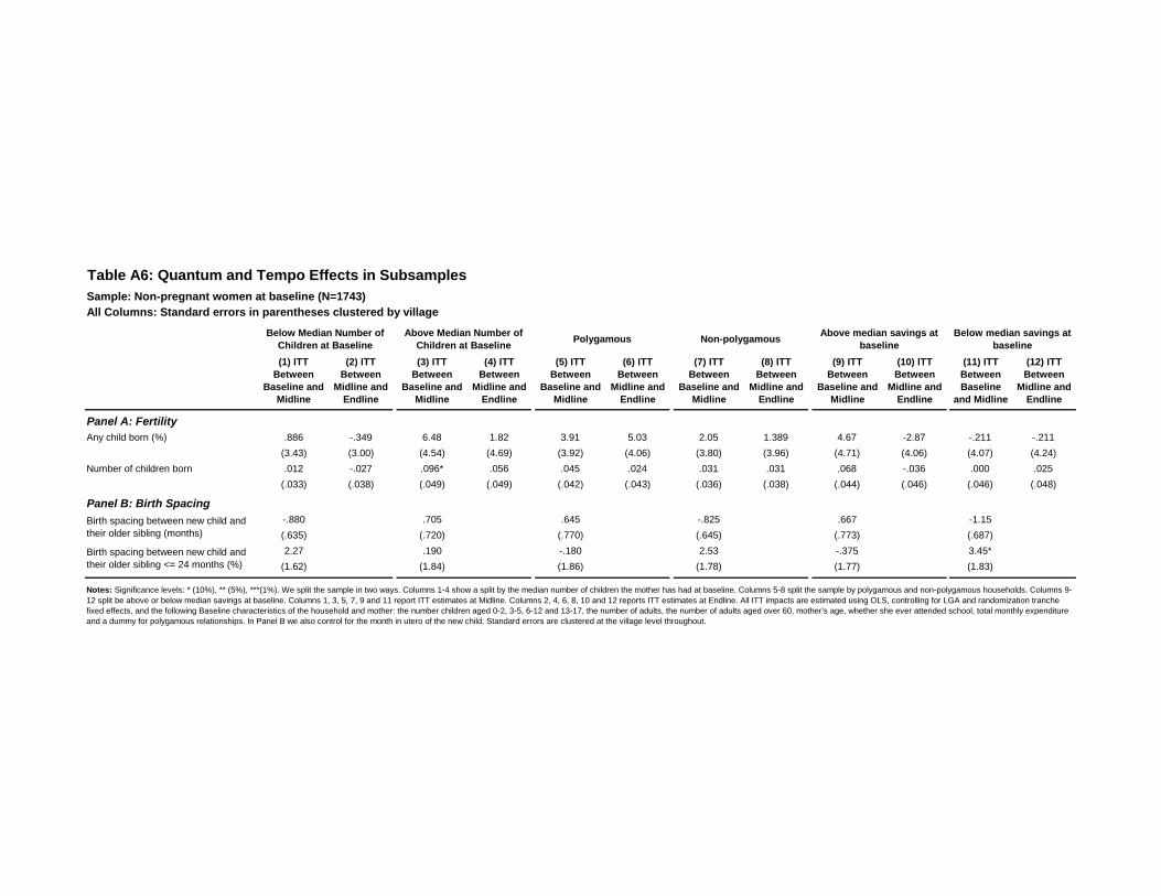
Table A6: Quantum and Tempo Effects in Subsamples

Sample: Non-pregnant women at baseline (N=1743)

All Columns: Standard errors in parentheses clustered by village

(1) ITT

Between

Baseline and

Midline

(2) ITT

Between

Midline and

Endline

(3) ITT

Between

Baseline and

Midline

(4) ITT

Between

Midline and

Endline

(5) ITT

Between

Baseline and

Midline

(6) ITT

Between

Midline and

Endline

(7) ITT

Between

Baseline and

Midline

(8) ITT

Between

Midline and

Endline

(9) ITT

Between

Baseline and

Midline

(10) ITT

Between

Midline and

Endline

(11) ITT

Between

Baseline

and Midline

(12) ITT

Between

Midline and

Endline

Any child born (%) .886 -.349 6.48 1.82 3.91 5.03 2.05 1.389 4.67 -2.87 -.211 -.211

(3.43) (3.00) (4.54) (4.69) (3.92) (4.06) (3.80) (3.96) (4.71) (4.06) (4.07) (4.24)

Number of children born .012 -.027 .096* .056 .045 .024 .031 .031 .068 -.036 .000 .025

(.033) (.038) (.049) (.049) (.042) (.043) (.036) (.038) (.044) (.046) (.046) (.048)

-.880 .705 .645 -.825 .667 -1.15

(.635) (.720) (.770) (.645) (.773) (.687)

2.27 .190 -.180 2.53 -.375 3.45*

(1.62) (1.84) (1.86) (1.78) (1.77) (1.83)

Above median savings at

baseline

Below median savings at

baseline

Notes: Significance levels: * (10%), ** (5%), ***(1%). We split the sample in two ways. Columns 1-4 show a split by the median number of children the mother has had at baseline. Columns 5-8 split the sample by polygamous and non-polygamous households. Columns 9-

12 split be above or below median savings at baseline. Columns 1, 3, 5, 7, 9 and 11 report ITT estimates at Midline. Columns 2, 4, 6, 8, 10 and 12 reports ITT estimates at Endline. All ITT impacts are estimated using OLS, controlling for LGA and randomization tranche

fixed effects, and the following Baseline characteristics of the household and mother: the number children aged 0-2, 3-5, 6-12 and 13-17, the number of adults, the number of adults aged over 60, mother’s age, whether she ever attended school, total monthly expenditure

and a dummy for polygamous relationships. In Panel B we also control for the month in utero of the new child. Standard errors are clustered at the village level throughout.

Polygamous Non-polygamousAbove Median Number of

Children at Baseline

Below Median Number of

Children at Baseline

Panel B: Birth Spacing

Birth spacing between new child and

their older sibling (months)

Birth spacing between new child and

their older sibling <= 24 months (%)

Panel A: Fertility

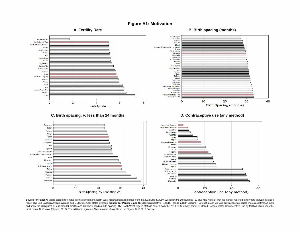
Figure A1: Motivation

A. Fertility Rate B. Birth spacing (months)

Source for Panel A: World bank fertility rates (births per woman), North West Nigeria statistics comes from the 2013 DHS Survey. We report the 20 countries (19 plus NW Nigeria) with the highest reported fertility rate in 2013. We also

report The Sub Saharan African average and OECD member states average. Source for Panels B and C: DHS Comparative Reports, Trends in Birth Spacing. For each graph we take any numbers reported more recently than 2000

and show the 20 highest % less than 24 months and 20 lowest median birth spacing. The North West Nigeria statistic comes from the 2013 DHS survey. Panel D: United Nations (2019) Contraceptive Use by Method which uses the

most recent DHS wave (Nigeria, 2018). The additional figures in Nigeria come straight from the Nigeria DHS 2018 Survey.

C. Birth spacing, % less than 24 months D. Contraceptive use (any method)

PregBL PregBL-ML Not Preg at ML

Additional Meal in Preg 0.113 0.109 0.085

Attend Antenatal Care 0.315 0.315 0.266

Use Health Facilities 0.278 0.278 0.205

Breastfeed Immediately 0.192 0.183 0.181

Exclusive Breastfeeding 0.504 0.509 0.42

Complimentary Foods 0.328 0.335 0.222

Hygiene and Sanitation 0.397 0.398 0.362

Nutritious Food 0.594 0.592 0.474

PregBL PregBL-ML Not Preg at ML

Additional Meal in Preg 0.094 0.091 0.091

Attend Antenatal Care 0.325 0.327 0.298

Use Health Facilities 0.31 0.313 0.243

Breastfeed Immediately 0.162 0.152 0.135

Exclusive Breastfeeding 0.432 0.431 0.38

Complimentary Foods 0.252 0.258 0.173

Hygiene and Sanitation 0.398 0.397 0.363

Nutritious Food 0.541 0.549 0.477

Figure A2: Recall of Key Messages at Midline

A. Wife's Recall of Key Messages

B. Husband's Recall of Key Messages

Notes: This figure is based on data from women and their husbands in households. It shows the proportion of pregnant at baseline and not-pregnant at

baseline women and husband who recall the eight key messages at Midline. Recall is from any low intensity information channel (posters, radio, fooddemonstrations and health talks). Individuals are asked if they have been exposed to CDGP information from a particular information channel (and werepeat this for each channel). If the individual says yes to this, they are asked what messages do they recall from the information channel. If an individualwas not exposed to any information channel, their recall of messages is set to zero.

0

0.1

0.2

0.3

0.4

0.5

0.6

Additional Mealin Preg

Attend AntenatalCare

Use HealthFacilities

BreastfeedImmediately

ExclusiveBreastfeeding

ComplimentaryFoods

Hygiene andSanitation

Nutritious Food

PregBL PregBL-ML Not Preg at ML

0

0.1

0.2

0.3

0.4

0.5

0.6

Additional Meal inPreg

Attend AntenatalCare

Use HealthFacilities

BreastfeedImmediately

ExclusiveBreastfeeding

ComplimentaryFoods

Hygiene andSanitation

Nutritious Food

PregBL PregBL-ML Not Preg at ML

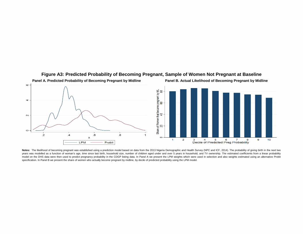
Figure A3: Predicted Probability of Becoming Pregnant, Sample of Women Not Pregnant at Baseline

Panel A. Predicted Probability of Becoming Pregnant by Midline Panel B. Actual Likelihood of Becoming Pregnant by Midline

Notes: The likelihood of becoming pregnant was established using a prediction model based on data from the 2013 Nigeria Demographic and Health Survey (NPC and ICF, 2014). The probability of giving birth in the next two

years was modelled as a function of woman’s age, time since last birth, household size, number of children aged under and over 5 years in household, and TV ownership. The estimated coefficients from a linear probability

model on the DHS data were then used to predict pregnancy probability in the CDGP listing data. In Panel A we present the LPM weights which were used in selection and also weights estimated using an alternative Probit

specification. In Panel B we present the share of women who actually become pregnant by midline, by decile of predicted probability using the LPM model.

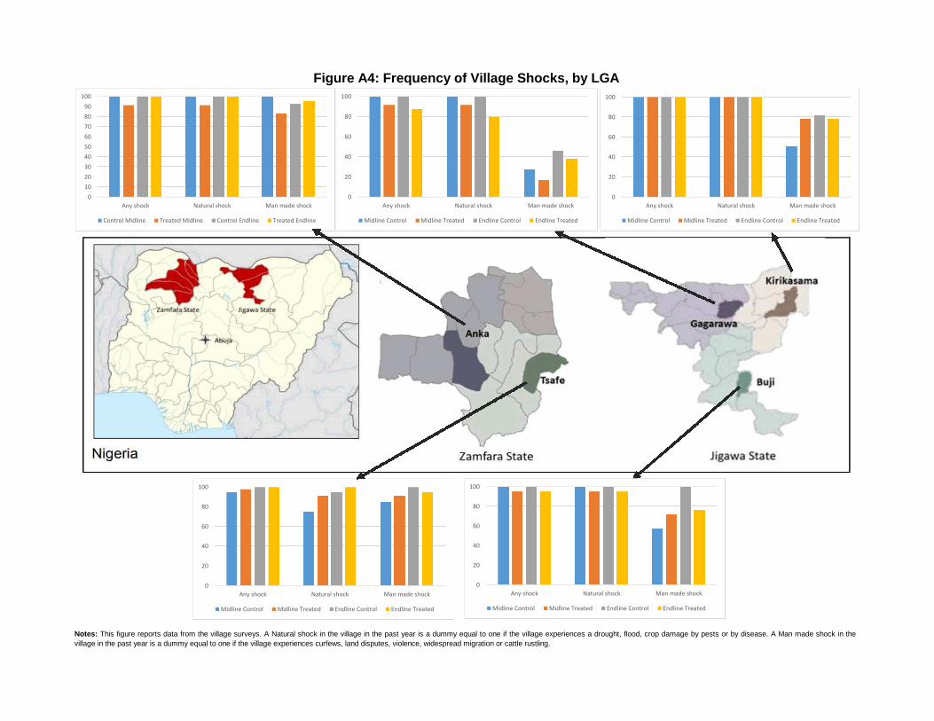
Anka

Any shock

Control Treated Control Treated Natural shock

Any shock 100 91.30435 100 100 Man made shock

Natural shock 100 91.30435 100 100

Man made shock 100 82.6087 92.85714 95.45455

Tsafe

Control Treated Control Treated

Any shock 95 97.72727 100 100

Natural shock 75 90.90909 94.44444 100

Man made shock 85 90.90909 100 94.44444

Buji

Control Treated Control Treated

Any shock 100 95.2381 100 95.2381

Natural shock 100 95.2381 100 95.2381

Man made shock57.14286 71.42857 100 76.19048

Kiri K

Control Treated Control Treated

Any shock 100 100 100 100

Natural shock 100 100 100 100

Man made shock 50 77.77778 81.81818 77.77778

Gagara

Control Treated Control Treated

Any shock 100 91.66667 100 87.5

Natural shock 100 91.66667 100 79.16667

Man made shock27.27273 16.66667 45.45455 37.5

Notes: This figure reports data from the village surveys. A Natural shock in the village in the past year is a dummy equal to one if the village experiences a drought, flood, crop damage by pests or by disease. A Man made shock in the

village in the past year is a dummy equal to one if the village experiences curfews, land disputes, violence, widespread migration or cattle rustling.

EndlineMidline

Figure A4: Frequency of Village Shocks, by LGA

Midline Endline

Midline Endline

Midline Endline

Midline Endline

0

10

20

30

40

50

60

70

80

90

100

Any shock Natural shock Man made shock

Control Midline Treated Midline Control Endline Treated Endline

0

20

40

60

80

100

Any shock Natural shock Man made shock

Midline Control Midline Treated Endline Control Endline Treated

0

20

40

60

80

100

Any shock Natural shock Man made shock

Midline Control Midline Treated Endline Control Endline Treated

0

20

40

60

80

100

Any shock Natural shock Man made shock

Midline Control Midline Treated Endline Control Endline Treated

0

20

40

60

80

100

Any shock Natural shock Man made shock

Midline Control Midline Treated Endline Control Endline Treated