do fiscal transfers alleviate business tax competition ... filedo fiscal transfers alleviate...

DO FISCAL TRANSFERS ALLEVIATE BUSINESS TAX COMPETITION? EVIDENCE FROM GERMANY

PETER EGGER MARKO KOETHENBUERGER

MICHAEL SMART

CESIFO WORKING PAPER NO. 1955 CATEGORY 1: PUBLIC FINANCE

MARCH 2007

An electronic version of the paper may be downloaded • from the SSRN website: www.SSRN.com • from the RePEc website: www.RePEc.org

• from the CESifo website: Twww.CESifo-group.deT

CESifo Working Paper No. 1955

DO FISCAL TRANSFERS ALLEVIATE BUSINESS TAX COMPETITION? EVIDENCE FROM GERMANY

Abstract The paper empirically analyzes the incentive effects of equalizing transfers on business tax policy by exploiting a natural experiment in the state of Lower Saxony which changed its equalization formula as of 1999. We resort to within-state and across-state difference-in-difference estimates to identify the reform effect on municipalities' business tax rates. Confirming the theoretical prediction, the reform had a significant impact on the municipalities’ tax policy in the four years after the reform with a “phasing out” of the effect starting in the fourth to fifth year. The finding is robust to various alternative specifications.

JEL Code: H71, H25.

Keywords: equalization grants, tax competition, local public finance, fiscal capacity equalization.

Peter Egger Ifo Institute for Economic Research

at the University of Munich Poschingerstr. 5 81679 Munich

Germany [email protected]

Marko Koethenbuerger Center for Economic Studies and CESifo

at the University of Munich Schackstr. 4

80539 Munich Germany

[email protected]

Michael Smart

Department of Economics University of Toronto

150 St. George St. Toronto ON M5S 3G7

Canada [email protected]

We are grateful for comments by seminar participants in Bergen (NHH, March 2006), Berlin (WZB, May 2006), Helsinki (HECER, October 2006), Paphos (IIPF meeting, August 2006), and Paderborn (July 2006). The usual disclaimer applies.

1 Introduction

It is a familiar shibboleth among public finance economists that decentral-ization of business taxation to lower-level governments can give rise to un-desirable competition for mobile tax bases, and a “race to the bottom” intax rates. Despite such concerns, a number of authors have recently ob-served that a system of intergovernmental transfers similar to those exist-ing in many countries may in principle serve as a corrective device for localbusiness tax competition, discouraging beggar-thy-neighbor tax policies andeven under some conditions guaranteeing the efficiency of decentralized poli-cies.

Under such transfer systems, known as capacity equalization or foun-dation grants, each government receives a transfer equal to the differencebetween its measured tax base and either the average base of all regionsor a measure of fiscal needs, multiplied by some target tax rate. Thus acapacity equalization grant is an equity-enhancing device that insures thateach jurisdiction can achieve some target level of spending determined byfederal authorities, as long as it sets its own tax rate at least as high as thetarget level.1 As Smart (1998) and Kothenburger (2002) observed, however,an increase in local tax rates causes measured tax bases to decline, as tax-payers shift to other regions of the country or to other, more lightly taxedactivities—and so causes capacity equalization transfers to rise. Thus thegrants in effect subsidize tax increases and penalize tax cuts by local govern-ments, and the effect is larger the greater is the equalization rate (sometimesreferred to as “taxback rate”) at which deficiencies in local fiscal capacityare compensated through the transfer formula.2

In this paper, we look for empirical evidence of the effects of equalizationgrants on local tax policy using data on a large set of German municipalities.The German case is an especially interesting one to examine, since munici-palities there levy a tax on resident businesses, known as Gewerbesteuer, atrates that average about 16 per cent of incomes. Since interjurisdictionalmobility and the pressures of tax competition in such a setting should inprinciple be high, the equalization grants system may play an important, if

1The capacity equalization principle currently forms the basis for transfer systems inAustralia, Canada, Germany, and Switzerland, as well as local school district financeformulas in many US states.

2This effect is clearest when considering a receiving region with a tax rate equal tothe target tax rate at which capacity deficiencies are compensated: At this point, furtherincreases in the rate will appear to create no deadweight loss to the region, as the increasein equalization transfers exactly compensates for marginal losses in private consumption.Thus equalization tends to drive tax rates above the target tax rate.

2

unintended, role in maintaining current rates of taxation.Our empirical approach relies on differences in tax-setting incentives fac-

ing municipalities that qualify for the systems of “regular” and “supplemen-tary” equalization transfers, and in particular the court-ordered reforms ineligibility for supplementary transfers that occurred in the state of LowerSaxony (Niedersachsen) in 1999. Regular equalization transfers are availableto municipalities whose fiscal capacity falls below a target level, while sup-plementary transfers are targeted at municipalities with considerably lowerthan average fiscal capacity. About three-quarters of the 1022 municipalitiesin Lower Saxony receive one or both types of equalization transfers. The ef-fect of the 1999 reform was to reduce the equalization rate facing municipal-ities eligible for supplementary transfers, while increasing the equalizationrate for other, ineligible municipalities. The former group of municipali-ties is therefore hypothesized to levy lower tax rates than the latter one inresponse to the reform.

Since the equalization formula itself implicitly defines the sets of munic-ipalities that are eligible and ineligible for supplementary grants, identifica-tion of incentive effects of equalization must address the inherent problemsof self-selection. The reason is that a jurisdiction can to some extent influ-ence the fiscal capacity and thus the program type it is eligible for. Thecorresponding equalization transfer eligibility and tax policy are then bothendogenous. This may generate a bias with simple mean comparison esti-mates of a transfer reform on the tax setting of the eligible municipalitiesrelative to the non-eligible ones. To avoid this bias, we address the problemof self-selection by applying switching regression and matching proceduresin the empirical analysis.

Two sources of heterogeneity enable the identification of the reform ef-fect on tax rates. First, to the extent that municipalities respond heteroge-neously to a change in supplementary transfers within a federal union (asthe reform entails for municipalities in Lower Saxony), the differential effectcan be estimated using differences in business tax policy between the sub-sample of supplementary transfer recipients and an appropriate within-statecontrol group. The construction of the latter group should pay attention tothe problem of self-selection into supplementary transfer eligibility. Second,since municipal equalization schemes differ among German states (Lander),one can identify the effect of a transfer reform by comparing the changein tax policy between municipalities in the reforming and a non-reformingstate. In our analysis, we estimate the reform effect on municipalities inLower Saxony by a comparison with the 2056 municipalities in the state ofBavaria, which experienced no reform in the equalization system over our

3

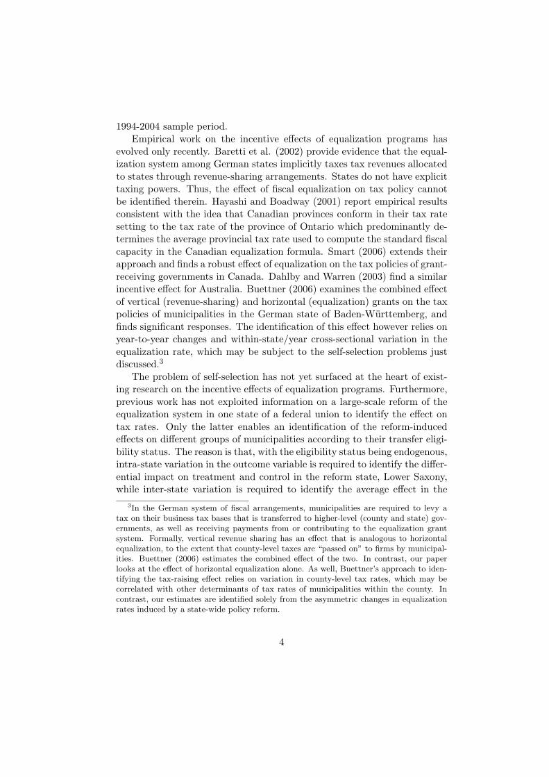
1994-2004 sample period.Empirical work on the incentive effects of equalization programs has

evolved only recently. Baretti et al. (2002) provide evidence that the equal-ization system among German states implicitly taxes tax revenues allocatedto states through revenue-sharing arrangements. States do not have explicittaxing powers. Thus, the effect of fiscal equalization on tax policy cannotbe identified therein. Hayashi and Boadway (2001) report empirical resultsconsistent with the idea that Canadian provinces conform in their tax ratesetting to the tax rate of the province of Ontario which predominantly de-termines the average provincial tax rate used to compute the standard fiscalcapacity in the Canadian equalization formula. Smart (2006) extends theirapproach and finds a robust effect of equalization on the tax policies of grant-receiving governments in Canada. Dahlby and Warren (2003) find a similarincentive effect for Australia. Buettner (2006) examines the combined effectof vertical (revenue-sharing) and horizontal (equalization) grants on the taxpolicies of municipalities in the German state of Baden-Wurttemberg, andfinds significant responses. The identification of this effect however relies onyear-to-year changes and within-state/year cross-sectional variation in theequalization rate, which may be subject to the self-selection problems justdiscussed.3

The problem of self-selection has not yet surfaced at the heart of exist-ing research on the incentive effects of equalization programs. Furthermore,previous work has not exploited information on a large-scale reform of theequalization system in one state of a federal union to identify the effect ontax rates. Only the latter enables an identification of the reform-inducedeffects on different groups of municipalities according to their transfer eligi-bility status. The reason is that, with the eligibility status being endogenous,intra-state variation in the outcome variable is required to identify the differ-ential impact on treatment and control in the reform state, Lower Saxony,while inter-state variation is required to identify the average effect in the

3In the German system of fiscal arrangements, municipalities are required to levy atax on their business tax bases that is transferred to higher-level (county and state) gov-ernments, as well as receiving payments from or contributing to the equalization grantsystem. Formally, vertical revenue sharing has an effect that is analogous to horizontalequalization, to the extent that county-level taxes are “passed on” to firms by municipal-ities. Buettner (2006) estimates the combined effect of the two. In contrast, our paperlooks at the effect of horizontal equalization alone. As well, Buettner’s approach to iden-tifying the tax-raising effect relies on variation in county-level tax rates, which may becorrelated with other determinants of tax rates of municipalities within the county. Incontrast, our estimates are identified solely from the asymmetric changes in equalizationrates induced by a state-wide policy reform.

4

reform state (across state difference in difference analysis).We find a significant effect of the reform on local business tax rates. As

hypothesized, tax rates in eligible municipalities fell gradually in the fouryears following the reform, relative to ineligible municipalities’ rates. Theoverall impact on the gap in business tax rates amounted to about 0.95percentage points, about five percent of their original level. This estimatedaverage treatment effect however masks important heterogeneity in responseto the reform. According to our estimates, the magnitude of the estimatedexogenous treatment effect is downward biased by about 83 percent. Onthe basis of the between-state difference in difference analysis, moreover, weconclude that the reform raised the average level of taxes in the reform state.These results are robust to alternative choices of the estimation proceduresand the inclusion of alternative control variables.

The remainder of the paper is organized as follows. Section 2 developsthe theoretical hypotheses. Section 3 reviews the features of the Germanmunicipal equalization system and explains the reform effects from a theo-retical perspective. The data are presented in Section 4, while Sections 5and 6 summarize the empirical strategy and the results. The last sectionconcludes with a summary of the major findings.

2 Equalization and tax competition

To understand the incentive effects of equalization grants, consider a versionof the model in Kothenburger (2002) and Bucovetsky and Smart (2006). Afederation consists of two jurisdictions, labelled i and j, each with a singleresident and a single tax base. Jurisdiction i levies tax rate τi on its ownbase Bi. Let the tax base in jurisdiction i be a linear function of tax ratesin the federation,

Bi = B0i + cτj − aτi (1)

where B0i and a > c ≥ 0 are parameters. Thus the model incorporates a

fiscal spillover (e.g. tax competition where Bi is the capital tax base) amongjurisdictions when c > 0, since a rise in the tax rate in one jurisdiction causesa rise in the other jurisdiction’s tax base.

Each jurisdiction receives from the central government an equalizationgrant that compensates for differences in the size of the local tax bases. Forjurisdiction i, the transfer formula is

Ti = αi (Ni −Bi) , (2)

5

where Ni is a parametric lump-sum component to the grant representing thejurisdiction’s deemed “fiscal need”, and αi is the rate at which the grant isreduced for each unit of local fiscal capacity or tax base Bi. (The variablesfor jurisdiction j are defined analogously.) Note that we allow marginalequalization rates αi to differ between jurisdictions; capturing the possibilitythat jurisdictions operate on different segments of a non-linear equalizationscheme. In particular, this subsumes the case in which one jurisdiction is noteligible for equalization transfers (αi = 0), perhaps because it has exogenousfiscal capacity that exceeds deemed fiscal need, while the other jurisdictionremains eligible for equalization payments (αj > 0).

Consider the problem of a government in region i that seeks to maximizerevenue net of federal equalization transfers, and which takes the parametersof the equalization formula and the tax rate of the other jurisdiction asgiven.4 In this model, the optimal tax rate τi solves

max τiBi + αi (Ni −Bi)

for which the first-order (necessary and sufficient) condition is

Bi − a(τ∗i − αi) = 0. (3)

The first-order condition defines the optimal tax rate in region i as a func-tion of the neighbor region’s tax rate and its marginal equalization rate,τ∗i (τj , αi). Using (1) comparative statics on τi yields an inverse relationshipbetween τi and region i’s marginal equalization rate αi.

In the empirical analysis below, we examine the impact of the equaliza-tion formula on the reduced form tax rates of affected governments, withoutregard for the structural interactions among tax rates as embodied in thereaction function τ∗i (τj , αi). To motivate this approach, therefore, we maysolve for the Nash equilibrium tax rates of the jurisdictions that consti-tute a fixed point of the reaction functions. This can be interpreted as areduced form relationship between tax rates and equalization parameters,τ∗i (αi, αj).5 Our empirical work employs a “difference-in-difference” strat-

4The Leviathan assumption together with the linearity of the tax base in (1) greatlysimplifies the analysis, while preserving the essential features of the incentive effects ofequalizing transfers. The linear model was studied by Bucovetsky (1991) inter alia. Theeffect of equalization transfers on welfare maximizing governments facing non-linear taxbases is addressed in Smart (1998), and the qualitative results are the same.

5Following the first-order condition, the reduced form relationship is

τ∗i =2a

4a2 − c2

�B0

i + aαi

�+

c

4a2 − c2

�B0

j + aαj

�. (4)

Observe that a > c ≥ 0 is sufficient to guarantee existence of a unique Nash equilibrium.

6

egy that examines how the tax rates of jurisdictions change relative to eachother in response to a change in their relative marginal rates of equalization.To see this relationship in the theoretical model, we may therefore computethe difference in equilibrium tax rates

τ∗i − τ∗j =B0

i −B0j

2a + c+

a

2a + c(αi − αj) ≡ βij + γ(αi − αj). (5)

The tax differential is positively related to the differential in equalizationrates pertaining to the respective jurisdictions.

3 Equalization transfers in Germany

In describing the municipal equalization scheme, we focus on the system inLower Saxony where a reform has been implemented as of 1999.

The core of the municipal transfer system is: (i) a system of “regular”equalization grants, which compensate for a fraction of the amount by whicheach municipality’s measured taxation capacity falls short of its targetedspending level or “fiscal need”, and (ii) a system of supplementary equaliza-tion grants, which establish a floor level of spending in each municipality,and equalize 100 per cent of deficiencies up to the floor.

In algebraic terms, let Bi denote the measured tax capacity in munic-ipality i; that is, the revenues that would be available for local spendingpurposes if the jurisdiction were to levy a centrally determined reference taxrate on its measured tax bases.6 Let Ni denote the “fiscal need” or targetspending level of the municipality–again, a centrally determined parameterthat depends only on the current population of the municipality. Let αbe the rate at which capacity deficiencies are compensated under the regu-lar equalization transfer. Finally, let βNi denote the spending floor belowwhich deficiencies are fully compensated under the supplementary equal-ization transfer, where β is a centrally (state-level) determined parameterthat is common to all municipalities within the same state. The aggregateequalization transfer to the municipality may then be written:

Ti(Bi) = α max{Ni −Bi, 0}+ max{βNi −Bi − α(Ni −Bi), 0} (6)6In practice the fiscal capacity is the jurisdiction’s tax base multiplied by a “standard”

tax rate. In the sequel we assume a “standard” tax rate equal to unity. Since its level hasno formulaic relation to the municipalities’ business tax rate choices, the simplificationdoes not impair the analysis of incentive effects.

7

Figure 1: Equalization transfers and incentives.

where the first term corresponds to the regular equalization transfer andthe second to the supplementary transfer (which itself depends on the fiscalcapacity resulting from the regular transfer).7

Observe that the second term in the transfer formula, the supplementaryequalization component, is positive if and only if (β−α)Ni− (1−α)Bi > 0or

Bi <β − α

1− αNi ≡ θNi (7)

where θ < 1. Thus θ in (7) expresses the fraction of target spending belowwhich capacity deficiencies are fully equalized.

This describes the state’s horizontal equalization system in general terms7In the transfer system described by equation (6), equalization is on a “gross” basis:

each transfer is positive if the corresponding deficiency is positive, and zero otherwise;municipalities with capacity in exceed of fiscal need are not taxed under the formula. Infact, in the 1999 Lower Saxony reform discussed below, municipalities with excess capacitywere required to pay 20 per cent of the difference to the state government, converting theactual formula to a partial “net” equalization basis. We return to this issue below.

8

throughout our sample period. We turn now to the numerical values as-sumed by the parameters in the formula and the changes in the parametersfollowing the 1999 reform—which is the key to our identification strategy.The reform was initiated by a ruling of the state supreme court in November1997 which declared the initial system unconstitutional and requested theimplementation of a new system as of 1999. The reform prescribed changesin the different equalization rates. Prior to the reform, the regular equal-ization transfer compensated 50 per cent of deficiencies in capacity belowthe target level, and the spending floor was established at 80 per cent ofthe target level; thus α0 = 1/2 and β0 = 4/5 in the pre-reform period,and θ0 = (4/5 − 1/2)/(1/2) = 3/5 was the threshold fraction of the tar-get below which supplementary equalization was paid. In the 1999 reform,the regular equalization was increased to 75 per cent, while other param-eters of the formula remained unchanged; thus α1 = 3/4, β1 = 4/5, andθ1 = (4/5 − 3/4)/(1/4) = 1/5. As we will see, this resulted in substantialchanges in municipal government incentives.

To understand the incentives for local tax policy induced by the transfersystem, it is useful to consider the graph of the equalization formula. Figure1 expresses the relationship between a municipality’s own fiscal capacity Bi

and its equalization transfers Ti(Bi) in both the pre-reform and post-reformperiods. The kinked line segment ADNG is the constraint which obtainsin the pre-reform period: capacity deficiencies are fully compensated bytransfers when Bi ≤ θ0Ni, so the constraint has slope -1 in this interval;50 per cent of capacity deficiencies are compensated when θ0Ni < Bi ≤ Ni,so the slope of the constraint is -0.5 in this interval; and no equalizationtransfers are paid when Bi > Ni, the slope of the constraint is thus zeroto the right of Ni. The post-reform budget constraint is represented bythe kinked line segment ACNH. The effect of the reform was to increasethe fraction of capacity deficiencies compensated by regular equalizationtransfers to 75 per cent and so to increase the slope of the constraint by 0.25(in absolute value) in the intermediate interval, while reducing the thresholdat which supplementary equalization was paid commensurately to θ1Ni.8

For governments with tax capacity in excess of need, operating on segmentNG, no equalization payments were received before or after the reform. In

8For governments initially operating on segment AC of the pre-reform constraint, therewas no change in marginal incentives. Observe however that the new threshold level wasextremely low, at 20 per cent of the target spending level. In consequence, only onemunicipality has qualified for supplementary transfers in the post-reform period. Wecategorize this municipality as part of the treatment group 1 despite the fact that therewas no change in marginal incentives; this can only lead to attenuation bias in our results.

9

the post-reform period, however, such municipalities were required to pay20 per cent of excess tax capacity to the state government, operating nowon the segment NH with slope -0.2. Such a payment operates exactly like anegative equalization grant with an equalization fraction of one-fifth.

Thus the reform resulted in a rather stark change in the extent to whichmarginal changes in local resources Bi are compensated through the formula.Municipalities may be classified into three groups based on their equalizationstatus prior to the reform. Group 1, corresponding to segment CD of thepre-reform budget constraint, faced a decrease in equalization fraction of 25percentage points following the reform, while Groups 2 and 3, correspondingto segments DN and NG, faced increases in the equalization fraction of 25and 20 percentage points, respectively. According to our theory then, taxrates among the former group of governments are predicted to fall, comparedto those of the other two groups.

It is this shock to incentives that is the key to our identification strategy,described in further detail below. An obvious concern with this approach isthat factors that determine the initial equalization status of a municipalitymay be related to the unobservable determinants of subsequent innovationsin tax rates, so that assignment to treatment and control groups is notignorable in our analysis. We describe our strategy for dealing with theendogeneity issue in Section 5.

4 Data

We use data on municipalities in the state of Lower Saxony over the timeperiod 1994 - 2004. The described reform in Lower Saxony was effective asof 1999. We use data on the business tax rate which is set at the munic-ipal level in Germany, information on the transfer formula as given in (1)before and after the reform for each municipality in Lower Saxony, and socio-economic characteristics of the respective municipalities such as population(inhabitants, age structure, and population density), income per capita, andthe unemployment rate. Also, we account for geographical characteristicsof a municipality (land used for agriculture, forests, water sheds, and sizeof the road network each of which is measured in hectares). Finally, weemploy political characteristics such as the party composition of the localgovernment (social democrats, liberals, conservatives, and the greens). Alldata except unemployment rates are available from the respective statisti-cal office (Statistische Landesamt), most of it is available in a on-line data

10

base.9 Data on the number of unemployed at the municipal level are takenfrom the Federal Labor Office (Bundesagentur fur Arbeit) - also availableon-line.10

In some of our estimations, we will employ data on Bavarian munici-palities as a control group. In Bavaria, the reform described in Section 3did not take place. The corresponding socio-economic, geographical andpolitical data come from the Bavarian statistical office.11 Again, the unem-ployment rates are taken from the Federal Labor Office (Bundesagentur furArbeit).

In the subsequent analysis, we consider all municipalities in Lower Sax-ony as supplementary transfer eligible ones if they have actually receivedsuch transfers in at least one year in the pre-reform period (1994-98). In allestimations, the remaining Lower Saxony municipalities belong to the con-trol group. Table 1 provides details on the number of eligible and non-eligiblemunicipalities, the average business tax rate, the average fiscal capacity percapita as defined by the equalization formula, and the average income percapita across years and municipalities in the respective group.12

About three quarters of the 1022 municipalities in Lower Saxony weresupplementary transfer eligible in at least one year between 1994 and 1998.The income per capita level is slightly lower in eligible municipalities than innon-eligible ones. On average, they applied a slightly lower business tax ratethan their non-eligible counterparts, and their fiscal capacity is significantlylower. To give a first impression of the possible response of tax rates tothe reform, we illustrate the development of the business tax rates in LowerSaxony in Figure 2. The vertical bar in the figure indicates the end of thelast pre-reform year 1998. Business tax rates in this and earlier years wereabout 0.15 percentage points higher in non-eligible municipalities than ineligible ones. This is also consistent with the information given in Table 1.Before the reform, there was not much change in this relationship. But thefigure suggests that the gap in the two tax rates increased immediately afterthe reform year. The adjustment in the gap is somewhat sluggish and a new’steady-state’ in the gap seems to be reached only after four years.

The information in Figure 2 may also be inferred from a descriptivecomparison along the lines of regression analysis. In Table 2 we consider the

9The link is http://www1.nls.niedersachsen.de/Statistik/.10The link is http://www.pub.arbeitsamt.de.11The link is https://www.statistikdaten.bayern.de.12The income per capita seems low, but note that the denominator includes all inhab-

itants of a municipality, irrespective of whether they are working, unemployed, or not inthe labor force at all.

11

15

15,25

15,5

15,75

16

16,25

16,5

16,75

17

1994 1995 1996 1997 1998 1999 2000 2001 2002 2003 2004

Average municipality noteligible for supplementary

transfers

Average municipalityeligible for supplementary

transfers

%

Reform in LowerSaxony as of 1999

Figure 2: Average business tax rates of eligible and non-eligible municipali-ties in Lower Saxony.

average business tax rate in the period 1994-97 in eligible versus non-eligiblemunicipalities and compare it to any later year, capturing supplementarytransfer eligibility by a dummy variable that is set at one for eligible munic-ipalities and at zero for non-eligible ones. Of course, since 1998 was actuallynot covered by the reform the change in the eligible regions should be aslarge as in the non-eligible ones so that the gap does not increase. Hence,the coefficient of the eligibility status dummy variable should be close to zerofor 1998. In the subsequent periods, the increase in the gap should show upin an increasingly negative coefficient of the dummy variable of interest.

We find, consistent with Figure 2, that the gap opens up in 1999 (hence,here is no indication of anticipation effects in 1998), reaching a level of about-0.25 percentage points from 2003 onwards. The regression representationwill be useful for a comparison with the results in the subsequent analysis,where we account for a possible self-selection into supplementary transfereligibility. The latter seems particularly important for municipalities oper-ating next to the kinks of the budget constraint depicted in Figure 1. Forthese, a small change in tax policy may significantly change the local slope

12

of the non-linear budget constraint.

5 Empirical strategy

5.1 The problem of self-selection into supplementary trans-fer eligibility

It will be useful to start with a few definitions for portraying the problemof identification of the supplementary transfer reform effect on business taxrates at the municipal level and the outline of the empirical strategy. Forconvenience, we will refer to the case of supplementary transfer recipientstatus by index 1 (treatment status) and to the non-recipient status by index0 (no-treatment status). The corresponding business tax rate of municipalityi with and without treatment status is τi,1 and τi,0, respectively. Sincewe will focus on differences in differences of the reform effect, it will beuseful to define the pre-to-post-reform change in business tax rates of thesupplementary transfer eligible units as ∆τi,1, and that one of the ineligibleones as ∆τi,0. Therein, ∆ is the difference operator across periods.

Notice that there are two treatments of interest, here: the reform effect,which may be viewed as being exogenous from the viewpoint of a munic-ipality, and the supplementary transfer status, which may be endogenous.Let us refer to the binary supplementary transfer eligibility treatment formunicipality i as Zi with Zi = 1 in the treatment case (as Bi < θ0N inFigure 1) and Zi = 0 otherwise. Let us first focus on differences in businesstax rates between the pre- and post-reform periods for Lower Saxony munic-ipalities only. Then, we see that average effect of the exogenous treatment,namely the supplementary transfer reform, is simply a constant. However, incase of an endogenous selection of municipalities into supplementary trans-fer eligibility status, the change in business tax rates between the pre- andpost-reform periods will depend on this endogenous selection. Providing aconsistent identification of both the main reform effect and its interactioneffect with the status of transfer eligibility on business tax rates (∆τ1−∆τ0)is central to the paper.

The econometrics literature emphasizes the role of two core conceptsof treatment effects: the average treatment effect (see Rubin, 1983) beingdefined as ATE ≡ E[∆τ1 − ∆τ0], where, in our case, ∆τ1 and ∆τ0 arerandom vectors of changes in business tax rates from the population ofmunicipalities of interest; and the average treatment effect on the treated(see Heckman, 1997), being defined as ATT ≡ E[∆τ1 −∆τ0|Z = 1]. Hence,ATE is the unconditional, expected change in business tax rates associated

13

with the reform effect for a randomly drawn municipality. In contrast, ATTmeasures the expected treatment effect on a municipality that is randomlydrawn only from the sub-population of the actually supplementary transfereligible units.

If the supplementary transfer eligibility status were randomized acrossmunicipalities, Z would be independent of (∆τ1,∆τ0). Then, E[∆τ1 −∆τ0] = E[∆τ1 − ∆τ0|Z = 1] implying that ATE = ATT . Furthermore,the simple difference in the means of the pre-to-post-reform change in busi-ness tax rates among the eligible and ineligible municipalities13 is an un-biased, consistent, and asymptotically normal estimate of ATE and ATT.However, if municipalities internalize their possible influence on the slope ofthe budget constraint and adjust their tax rates accordingly, this creates aproblem of self-selection into treatment. Then, the assumption of a random-ized or exogenous treatment is not tenable anymore, rendering the simpledifference-in-means estimator of the reform-induced supplementary transfertreatment effect (of both ATE and ATT) on changes in business tax ratesbiased and inconsistent. Accordingly, the response to the tax reform can notbe estimated by an ordinary least squares approach as in Table 2 anymore.

5.2 Cures for self-selection

The micro-econometrics literature on program evaluation suggests severalalternative avenues of how to recover consistent estimates of ATE and ATTunder self-selection. Here, we focus on those approaches that involve theformulation of a non-linear probability model to estimate the endogenousselection into treatment (in our case, the probability that a municipality iseligible for supplementary transfers). We can think of the estimation of ATEor ATT as a two-stage problem, where the binary choice selection model isto be estimated in the first stage. In first stage regression, we determine theprobability of Z = 1 by a set of observable determinants. Let us refer to thelatter determinants as W, which is an N × k1 matrix, where N indicatesthe number of (treated plus untreated) observations in the sample, and k1

is the number of regressors included in the non-linear probability modelassuming either a normal or a logistic distribution function. In general,there are two possibilities to obtain consistent estimates of ATE or ATT. Oneinvolves the use of instrumental variable techniques (Wooldridge, 2002). Theother adopts the assumption of ignorability of treatment given the covariatescollected in W (Rosenbaum and Rubin, 1983). In the subsequent analysis,

13As is easily available from descriptive statistics or as a simple exogenous dummyvariable estimate in a regression of ∆τi on Zi (where ∆ is the difference operator).

14

we will in particular make use of the latter, while an application of theformer is relegated to the sensitivity analysis.

In our context, the assumption of ignorability of treatment given thecovariates entails that provided the correlation between the binary supple-mentary transfer eligibility Z and the business tax rate outcome (∆τ1, ∆τ0)can be eliminated by conditioning on W, we obtain consistent estimates ofATE and ATT.14 Two prominent approaches to estimate treatment effectsbased on the assumption of ignorability of treatment conditional on a setof observable variables15 are (i) selection control procedures based on theswitching regression model and (ii) matching based on the propensity score.

As an (intuitively appealing) alternative to the aforementioned proce-dures we can restrict the set of municipalities to those for which a self-selection problem is less of a concern, i.e. those which do not operate in theclose neighborhood of the kink D of the transfer formula depicted in Figure1. We present an analysis along these lines in section 6.3.

6 Results

6.1 Switching regression model

We first apply a switching regression model. Let us decompose the out-comes for the treated and the untreated municipalities (∆τk with k = 0, 1)into their mean (µk) and a stochastic part (νk), ∆τk = µk + νk. Then, wemay use the regression model ∆τ = µ0 + βZ + ε to estimate ATE, whereβ = (µ1 − µ0) reflects ATE and ε = ν0 + Z(ν1 − ν0) is an error term whichobviously depends on the supplementary transfer eligibility status Z. Sincethe business tax rate outcome ∆τ depends on Z, this is referred to as aswitching regression model. A two-step estimator that yields a consistentestimate of ATE can be obtained as follows. First, estimate the probabilityof being eligible for supplementary transfers depending on a set of instru-

14The assumption implies conditional mean-independence, which means that eventhough (∆τ1, ∆τ0) and Z are correlated (through self-selection), E[∆τ0|W, Z] =E[∆τ0|W] and E[∆τ1|W, Z] = E[∆τ1|W]. Hence, there is a set of observable vari-ables collected in W that can remove the correlation between (∆τ1, ∆τ0) and Z, and afterconditioning on W, we can obtain consistent estimates of ATE and ATT. Under condi-tional mean-independence, ATT conditional on W is defined as ATT (W) ≡ E[∆τ1 −∆τ0|W, Z = 1] and ATE conditional on W is defined as ATE(W) ≡ E[∆τ1 −∆τ0|W].Notice that ATT and ATE are identical under conditional mean-independence, and nofurther restrictions on joint or conditional distributions are required for identification.

15Due to the reliance on a set of observables, the approach is sometimes also referredto as selection on observables (Heckman and Robb, 1985; Moffitt, 1996).

15

ments W = [X,Y], where X is an N × k2 matrix of exogenous regressors inthe second stage model and Y is an N × k1 set of identifying instrumentsin the first stage model, with k1 denoting the number of regressors in thesecond stage. Second, determine the expected value of business tax ratesconditional on supplementary transfer eligibility, a set of exogenous vari-ables in the second stage model (collected in the matrix X), and on the setof instruments in the first stage (W) as:16

E(∆τ |Z,X,W) = α+βZ+Xγ+ρ1Zφ(Wδ)/Φ(Wδ)+ρ2Zφ(Wδ)/[1−Φ(Wδ)](8)

where Wδ = δ0 + Xδ1 + Yδ2. This is a generalized version of the Heck-man (1978) framework (Heckman’s estimator is based on a single parameterρ in the second stage model), which provides an unbiased, consistent, andasymptotically normal estimate of β (i.e., ATE) under standard assump-tions.17 Define νk = gk(X)+ek with E(ek,W) ∀k = 1, 0 referring to treatedand untreated municipalities, respectively, to indicate that (a, e0, e1) is in-dependent of W with a trivariate normal distribution by assumption. Then,ATE can easily be estimated by a two-stage procedure similar to the oneproposed by Heckman (1978): estimate a probit or logit model to obtainestimates of φ(Wδ) (i.e., the density of the standard normal evaluated atWδ) and Φ(Wδ) (i.e., the cumulative density of the standard normal eval-uated at Wδ); plug these estimates in the two inverse Mill’s ratios of thesecond stage linear regression model. Then, the coefficients of the two Mill’sratios ρk will control for the selection bias, rendering the estimates of ATEas captured by β unbiased, consistent, and asymptotically normal.

6.1.1 Propensity to be supplementary transfer eligible for LowerSaxonian municipalities

We assume that W consists of the following socio-economic and geograph-ical characteristics: a municipality’s area of agricultural land in hectares(as a measure of its degree of industrialization); the area of forest space inhectares; the area of watersheds in hectares (as a measure of remoteness);the area of paved streets in hectares (as a measure of a municipality’s infras-tructure endowment); per-capita GDP as of 1993 (i.e., in the pre-treatment

16Note that in the absence of Y ATE can still be identified if the non-linearity of thefirst-stage model is sufficiently informative (see Cameron and Trivedi, 2005).

17The assumptions are that functional forms are as indicated and that supplementarytransfer eligibility can be written as an indicator function of the form Z = 1[Wδ +a ≥ 0] and a is independently and identically distributed following a standard normaldistribution.

16

period); population size as of 1993; the change in population density betweenthe pre- and post-treatment periods; the share of the population below anage of 15 years as of 1993; and squared values of these eight variables. Hence,including the constant, the column rank of W is 17.

Most notably the geographical variables are hypothesized to influencethe fiscal capacity, but to be uncorrelated with the dependent variable ofthe second-stage regression which is the change in the tax rate following thereform. To illustrate the reasoning, return to the theoretical model of sec-tion 2. Consider the baseline component of municipality i’s tax base B0

i tosummarize the aforementioned variables; thus reflecting the municipality’spropensity to qualify for supplementary transfers. The equilibrium tax rateτ∗i depends on B0

i , while the change in a jurisdiction’s tax rate following areform of the equalization rates is independent of it - see (4).18 In section6.3 we perform sensitivity analysis with respect to the set of covariates sum-marized in W.

Table 3 provides a summary of the corresponding results for the selec-tion model determining the probability of supplementary transfer eligibility.It turns out that the squared variables are jointly significant and should beincluded. Six variables enter significantly, irrespective of whether we assumelogistically (in the logit) or normally distributed errors (in the probit). Inparticular, the probability of being treated as supplementary transfer eli-gible declines with the share of people below working age, and it declinesin the pre-treatment level of per-capita income. The likelihood of beingtreated is higher for regions with large water sheds. The reason is that theseregions are relatively remote. For both models, the pseudo R2 is fairly highregarding the sample size of 1022 observations and the fairly large numberof treated ones, amounting to about 0.26. The log-likelihood of the logitmodel is slightly higher than that one of the probit. However, the differenceis not significant according to a likelihood ratio test (this test is suggestedby Davidson and MacKinnon, 2004). In the subsequent analysis, we use theslightly preferable logit model throughout.

6.1.2 Switching regression estimates for Lower Saxony

The second stage results of the switching regression approach are depictedin Table 4. The estimates apply for a randomly selected municipality in

18Concretely, taking the difference of the equilibrium tax rate before and after the reform(i.e. for different values of αi and αj), the baseline components B0

i and B0j drop out.

17

the Lower Saxony sample, irrespective of whether it was eligible for sup-plementary transfers or not. We are primarily interested in the estimatespertaining to the effect of supplementary transfer eligibility. These are to beinterpreted as tax rate changes (pre and post reform period) of the eligiblemunicipalities relative to those of non-eligible ones. They correspond to thechange in the tax rate gap between eligible and non-eligible municipalities- similar to the illustration in Figure 2. As the pre-reform tax rate we takethe 1993/1997 average. Since the fiscal adjustment to the reform might besluggish, we estimate the corresponding ATE for each post-reform year sep-arately. Also, we check for possible anticipation effects by assigning 1998 tothe post-reform period. Recall, the reform became effective as of 1999 aftera supreme-court ruling in November 1997.

One concern with treatment estimates is that they might capture theimpact of omitted variables. To avoid this problem, we additionally controlfor covariates in the second stage (outcome) regression. Recall that the ma-trix of covariates has been referred to as X in Section 6.1 and, apart froma constant and the endogenous supplementary transfer eligibility in LowerSaxony, it collects the following determinants: the change in populationsince 1993/1997; the change in population density; the area of streets inhectares; the change in per-capita income since 1993/1997; and the changein the share of elderly people (with an age of more than 65 years).

We have experimented with less parsimonious specifications than theone reported in Table 4. In particular, we have checked for the possiblerelevance of unemployment rates, and other socio-economic and geographicalcharacteristics accounted for in the selection model. However, it turns outthat the less parsimonious model estimates are not significantly preferableto the ones in the table. In particular, population density and the size ofthe road network are the most important control variables according to theirsignificance.

Similar to the exogenous ATE estimates in Table 2, there is no indica-tion of significant anticipation effects in 1998 with the endogenous treatmentapproach. Put differently, the identified gap by 2003/2004 between the eli-gible and non-eligible municipalities is three times larger than its exogenouscounterpart. Recall that the reference estimate was about -0.25 percentagepoints in Table 2 whereas it amounts to -1.20 in the switching regression -see Table 4. However, one may argue that most of the difference in the esti-mates reflects an omitted control variables bias rather than a self-selectionbias in Table 2. It turns out that this is not the case. We illustrate thisissue in Figure 3.

18

-1,200

-1,000

-0,800

-0,600

-0,400

-0,200

0,000

1998 1999 2000 2001 2002 2003 2004

Endogenous average

treatment effect

Selection plus

omitted control

variables bias

Exogenous average treatment effect

(excl. controls)

Exogenous average treatment effect

(incl. controls)

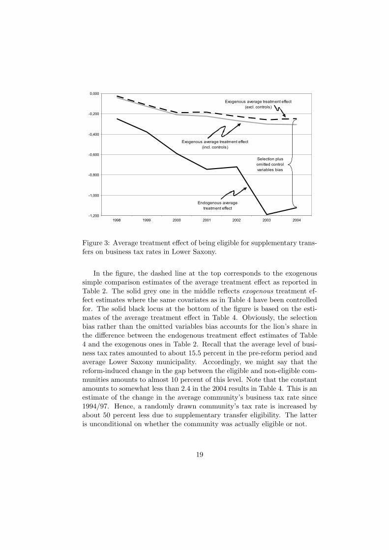
Figure 3: Average treatment effect of being eligible for supplementary trans-fers on business tax rates in Lower Saxony.

In the figure, the dashed line at the top corresponds to the exogenoussimple comparison estimates of the average treatment effect as reported inTable 2. The solid grey one in the middle reflects exogenous treatment ef-fect estimates where the same covariates as in Table 4 have been controlledfor. The solid black locus at the bottom of the figure is based on the esti-mates of the average treatment effect in Table 4. Obviously, the selectionbias rather than the omitted variables bias accounts for the lion’s share inthe difference between the endogenous treatment effect estimates of Table4 and the exogenous ones in Table 2. Recall that the average level of busi-ness tax rates amounted to about 15.5 percent in the pre-reform period andaverage Lower Saxony municipality. Accordingly, we might say that thereform-induced change in the gap between the eligible and non-eligible com-munities amounts to almost 10 percent of this level. Note that the constantamounts to somewhat less than 2.4 in the 2004 results in Table 4. This is anestimate of the change in the average community’s business tax rate since1994/97. Hence, a randomly drawn community’s tax rate is increased byabout 50 percent less due to supplementary transfer eligibility. The latteris unconditional on whether the community was actually eligible or not.

19

6.2 Matching based on the propensity score

In the previous analysis, we have focused on ATE, i.e. the treatment effectunconditional on actual treatment status. In fact, this is the (group size)weighted average of the ATT and the average treatment effect of the un-treated (ATU). In a next step, we address the effect on the actually treated,i.e. the ATT, by employing different matching estimates of the role of sup-plementary transfer eligibility for the tax reform effect in Lower Saxony.

Rosenbaum and Rubin (1983) deploy an estimate of the probabilityof treatment given the covariates W based on p(W) ≡ Prob(Z = 1|W).p(W) is the response probability (Φ(Wδ)), also referred to as the propen-sity score. p(W) serves as a metric to determine similar observations amongthe sub-samples of the treated and untreated observations (i.e., to constructa valid control group). Besides ignorability of treatment in the sense of con-ditional mean-independence, i.e., E(∆τk|W, Z) = E(∆τk|W) ∀k = 0, 1,the approach of propensity score matching hinges upon the assumptionthat 0 < p(W) < 1 (municipalities outside this support region have tobe dropped).19 Rosenbaum and Rubin (1983) refer to these two assump-tions together as strong ignorability of treatment. In this case, E[Z(∆τ |Z =1, p(W))] − E[Z(∆τ |Z = 0, p(W))] = E[Z(∆τ1 − ∆τ0)|p(W)]).20 Withmatching, the vector of predicted probabilities of being treated (as supple-mentary transfer eligible) is used to construct an appropriate control groupof ineligible municipalities with a similar probability of being eligible as theactually treated ones.

The most prominent matching procedure is nearest neighbor (or one-to-one) matching which works as follows: (i) determine a treated observation’sclosest ’twin’ in terms of the propensity score within the sub-sample of un-treated observations; (ii) compute the difference in the scores between thevector of treated and their matched twins; (iii) determine the average differ-ence which is an estimate of ATT. Alternatively, one could do the oppositeand match on each untreated observation its closest twin in the sub-sampleof treated ones. The latter would give an estimate of the average treatmenteffect of the ATU (in this case, we subtract the vector of business tax rates

19Hence, there is an implicit trade-off between goodness of fit in the selection modeland the number of observations that can be used for matching.

20Note that the use of a single indicator p(W) to determine the similarity of the treat-ment and control group involves a further assumption: namely that the two groups arenot only similar with respect to p(W) but also with respect to each and every determinantcollected in W. Otherwise, similarity in p(W) might be an artefact. Hence, matchingis only meaningful if we pass a test on the similarity of the observables included in theselection model.

20

of the matched treated from that one of the untreated). Then, ATE is noth-ing else than a sub-sample-size-weighted average of ATT and ATU. Hence,propensity score matching overcomes the bias associated with self-selectioninto treatment by determining a valid control group (see Rosenbaum andRubin, 1983, 1984, Abadie, 2005, Imbens, 2004) rather than removing theselection bias through the inclusion of inverse Mill’s ratios in a switchingregression model.

In general, the number of matched control units is either exogenouslyimposed (such as in the just described one-to-one matching) or a critical in-terval is determined with all unmatched municipalities in the correspondingprobability region around an eligible municipality’s predicted probability ofbeing treated. Some estimators even use a large amount or all untreatedunits as controls with their weight declining in the absolute difference toa treated unit’s predicted probability (the latter approach is referred toas kernel matching). In the baseline analysis we resort to nearest neigh-bor matching and employ alternative matching procedures in the sensitivityanalysis.

Nearest neighbor matching is based on the logit estimates in Table 3.The second stage estimates are given in the top panel of Table 5.

It is obvious that the ATT of the tax rate gap amounts to about -0.27(in 2002/2004) which is significantly smaller than ATE. This means thatan untreated municipality would have set a considerably smaller businesstax rate if it had been treated instead. Hence, the ATU is much larger inabsolute value than the ATT. The ATT is about as high as the exogenous,biased ATE. But the bias in the exogenous ATE is driven by the underlyingATU.

We report estimates of an alternative matching that involves the Bavar-ian municipalities as a control group in the bottom panel of Table 5. Withinthe 1994/2004 period the Bavarian state government kept the equalizationrates constant. The results suggest that the ATT in the larger sample isquite similar to its counterpart that is based on Lower Saxony municipali-ties only. This indicates that the matching quality is fairly good in either ofthe samples. However, the augmented data set allows us to gauge the ex-ogenous reform effect on the average Lower Saxony municipality besides itsinteraction effect with supplementary transfer eligibility. This is impossibleto infer based on the Lower Saxony data set where other, non-reform effectsenter the constant as well. Our findings suggest that the average LowerSaxony municipality had increased its tax rate by 1.16 percentage points by2003, compared to its Bavarian counterpart. The positive coefficient picks

21

up the reform-related incentive effect (some municipalities are hypothesizedto increase the tax rate), but also income effects on the average Lower Sax-ony municipality. Its interpretation may in principle also include significantnon-reform-related effects in the state of Bavaria which, however, we are notaware of.

As to the gap in tax rates between eligible and non-eligible municipalitiesin Lower Saxony, it increased by 0.26 percentage points over the same periodin accordance with the theoretical model.

6.3 Sensitivity analysis

We considered the robustness of the ATT estimates in several regards. First,even though the balancing property is not violated in our application,21 oneconcern might be that the exogenous variables in the selection model havean impact on the change in business tax rates on their own. Then, theyshould be controlled for in the matching models. Think of matching as aregression that includes a constant and the treatment dummy variable in asample that consists only of the treated and the control units (this samplewould be twice the number of treated observations with nearest neighbormatching). In principle, we can include other controls in this regression aswell (see Blundell and Costa Dias, 2002). This is done in the regressionswhose results are reported at the top of Table 6. The included covariatesare the same as in Table 3. Note that the results are very similar to thosein Table 5. Hence, we can conclude that there is no bias from omitting thecorresponding covariates in the second stage regression.

Second, there could be political covariates that could play a role instead.To account for this, we include the shares of the four parties (conservatives,social democrats, liberals, the greens) as possible determinants of changesin the business tax rates. Although some of the political variables entersignificantly in the regressions, the results are again very similar to theestimates in Table 5.

Third, we additionally account for the value added tax (VAT) whoserate is set by the federal government, while the proceeds are shared withmunicipalities. They may be thought of reflecting income effects. Althoughthe VAT enters significantly in some of the regressions, it does not changeour estimates of the ATT of the tax reform in Lower Saxony.

21Hence, the treatment and control group are not different with respect to the explana-tory variables in the selection model.

22

The first bloc of results in Table 6 refers to nonparametric matchingprocedures such as radius and kernel matching. Note that these rely ona larger sample of control municipalities than nearest neighbor matching.This results in an increase in efficiency but, in finite samples, the match-ing quality can be seriously smaller than with nearest neighbor matching.However, in our application the difference to the original estimates in Table6 is negligible. A second bloc of results provides the traditional Heckman(1978) two-step estimates. Note that these are based on a regression wherethe two Mill’s ratios (reported in Table 4) are forced to exhibit the samecoefficient. Not surprisingly, these estimates do not differ too much fromtheir ATE counterparts in Table 4. Finally, we apply two instrumental vari-able procedures suggested by Wooldridge (2002); i.e. Procedure 18.1 and avariant of Procedure 18.3. In contrast to the matching and the switchingregression model, instrumental variable procedures rest on relatively weakerassumptions regarding the available observable variables. However, they re-quire the existence of identifying instruments that are correlated with theselection indicator (the supplementary transfer eligibility), but not directlywith the outcome (the change in business tax rates). As explained above,the variables which are most notably uncorrelated with the outcome of thesecond-stage regression are the geographical variables of the first-stage re-gression. It turns out that the corresponding ATE estimates are very similarto the previous ones - see Table 6.

We undertake the same sensitivity analysis for the estimates that arebased on Lower Saxony and Bavaria - see Table 7. In general, the resultsare similarly robust as the previous ones (note that the bloc of results atthe top of Table 7 should be compared to the ones in the bottom panel ofTable 5). However, with the larger sample of Bavarian control units thenon-parametric (radius and kernel) matching estimators obviously lose inquality and cannot recommended any longer. Otherwise, the results aregenerally very robust in all considered respects.

In a final set of experiments, we change the specification of the probitmodel to investigate the sensitivity of the results in that regard. In Table8 we consider Lower Saxony municipalities only, and the results in Table 9are again based on the augmented sample including Bavarian municipalitiesin addition. In this analysis, we confine ourselves to two representative esti-mators: one-to-one matching as far as ATT is concerned, and Wooldridge’sProcedure 18.1 instrumental variable estimator regarding ATE.

We estimate three alternative probit models. The first one representsa rigorous second-order polynomial rather than only main effects and their

23

squared values as in Table 3. Hence, this specification also includes a com-prehensive set of interaction terms of the main effects as suggested by Rosen-baum and Rubin (1983). A second model only includes variables that arestrictly exogenous, at least in the medium run: namely the geographicalvariables such as agricultural land, forest land, and watersheds (simple andsquared values thereof).22 The third variant only relies upon populationand income variables variables in the pre-reform period: population, den-sity, income per capita, and the share of people with an age of less than15 years. With the specification based on geographical variables we obtainparameter estimates larger in absolute value than in the original specifica-tions. However, the general pattern of the estimated effects resembles thereference estimates.

An alternative way to deal with potential self-selection is to limit theeconometric analysis to those municipalities for which the problem is lessof a concern, i.e. which operate not too close to the kind D of the transferformula - see Figure 1. Constructing the treatment group, we exclude allmunicipalities that were potentially able to affect their eligibility status. Wedefine these municipalities as ones that had a lower ratio of the critical-to-actual fiscal capacity ratio than the average transfer receiving municipality(the critical fiscal capacity is centrally determined). Among the group ofnon-recipients, we treat those units as potentially being able to affect theireligibility status that had a higher ratio than the average non-recipient unit.After excluding these municipalities in each year, we estimate the regressionmodel underlying the results in Table 4. We obtain insignificant parameterestimates of 0.027 and -0.099 for 1998 and 1999, respectively. The parameterestimates for the years 2000-2004 are -0.148, -0.150, -0.206, -0.327, and -0.296. The estimates are significant at least at the five percent level. The sizeand pattern of the results is remarkably similar to the matching estimatesin Table 7.

7 Conclusion

Capacity equalization grants have been adopted in many countries primar-ily to affect interregional equity - but they may nevertheless influence local

22A reason for restricting the number of covariates in the binary choice model is thatmatching estimators include a bias term that declines at stochastic order (N − 1)/k, withN being the number of observations and k denoting the number of observables in theselection model. In small samples, this bias can be fairly large (see Frolich, 2004, Abadieand Imbens, 2006). With instrumental variable estimation, there is no presumption torely on a large number of identifying instruments, anyway.

24

policy incentives and the efficiency of the equilibrium tax system. Equal-ization grants calculate transfer entitlements indirectly, using differencesin revenues calculated at deemed rather than actual tax rates. But whenmeasured tax bases respond negatively to tax rate increases, this formulamay induce higher levels of taxation: increasing local tax rates causes mea-sured tax bases to decline, as economic activity shifts to other regions ofthe country or to other, more lightly taxed forms—and so causes capacityequalization transfers to rise. Thus the grants in effect subsidize increasesin taxes by equalization-receiving governments.

The paper empirically analyzes the incentive effects of equalizing trans-fers on business tax policy by exploiting a natural experiment in the state ofLower Saxony which changed its equalization formula as of 1999. Relying onwithin-state and across-state difference-in-difference estimates, the analysisreveals a significant impact of the reform on municipalities’ tax policy inthe four years after the reform with a “phasing out” of the effect starting inthe fourth to fifth year. The finding is robust to various alternative specifi-cations. The empirical result is in line with the theoretical prediction of apositive incentive effect of equalization grants on local tax rates.

From a policy perspective, the analysis suggests that fiscal capacityequalization implicitly acts as a tax coordination scheme, which deters mu-nicipalities from lowering taxes in order to attract a larger tax base (since itwould result in a reduction in transfers) and which therefore mitigates fiscalcompetition.23 Our reduced form approach does not allow us to determinethe extent to which the tax-raising effect of equalization is in fact mitigatedby the effects of fiscal competition among German municipalities that wouldotherwise have reduced consumer welfare. But this interpretation is in linewith the observation that the federal corporate tax rate fell from 56% onretained earnings and 36% on distributed earnings in 1980 to a uniformrate of 26.25% as of 2001 (in successive tax-cut cum base-broadening re-forms), a trend that is often attributed to intensified fiscal competition. Onthe other hand, municipal business tax rates on average did not fell overthe same period, suggesting that some mechanism – perhaps equalizationgrants—insulates these jurisdictions from fiscal competition.24

23Indeed, Kothenburger (2002) and Bucovetsky and Smart (2006) show that, in thepresence of horizontal tax competition, equalization grant may in a wide variety of settingsinduce subnational governments to independently choose tax rates that increase welfare.

24The federal corporate tax base is nearly perfectly co-occupied by the municipalities’business tax such that the broadening of the tax base does not account for the asymmetricresponse.

25

References

[1] Abadie, A. (2005), Semiparametric Difference-in-Differences Estima-tors, Review of Economic Studies 72(1), 1-19.

[2] Abadie, A. and G. Imbens (2006), Large Sample Properties of MatchingEstimators for Average Treatment Effects, Econometrica 74(1), 235-267.

[3] Baretti, C., B. Huber and K. Lichtblau (2002), A Tax on Tax Revenue:The Incentive Effects of Equalizing Transfers: Evidence from Germany,International Tax and Public Finance 9(6), 631-649.

[4] Blundell, R. and M. Costa Dias (2002), Alternative Approaches to Eval-uation in Empirical Microeconomics, Portuguese Economic Review 1,91-115.

[5] Bucovetsky, S. (1991), Asymmetric Tax Competition, Journal of UrbanEconomics 30(2), 167-181.

[6] Bucovetsky, S. and M. Smart (2006), The Efficiency Consequences ofLocal Revenue Equalization: Tax Competition and Tax Distortions,Journal of Public Economic Theory 8(1), 119-144.

[7] Buettner, T. (2006), The Incentive Effects of Fiscal Equalization Trans-fers on Tax Policy, Journal of Public Economics 90(3), 477-497.

[8] Cameron, A.C. and K.R. Trivedi (2005), Microeconometrics: Methodsand Applications, Cambridge University Press, New York.

[9] Dahlby, B., and N.A. Warren (2003), The Fiscal Incentive Effects of theAustralian Equalisation System, Economic Record 79(247), 434-445.

[10] Davidson, R. and J.G. MacKinnon (2004), Econometric Theory andMethods, University Press, Oxford.

[11] Frolich, M. (2004), Programme Evaluation with Multiple Treatments,Journal of Economic Surveys 18, 181-224.

[12] Hayashi M. and R. Boadway (2001), An Empirical Analysis of Inter-governmental Tax Interaction: The Case of Business Income Taxes inCanada, Canadian Journal of Economics 34, 481-503.

26

[13] Heckman, J.J. (1978), Dummy Endogenous Variables in a SimultaneousEquation System, Econometrica 46(4), 931-959.

[14] Heckman, J.J. and R. Richard Jr. (1985), Alternative Methods of Eval-uating the Impact of Interventions, in: James J. Heckman (ed.), Lon-gitudinal Analysis of Labour Market Data, Econometric Society Mono-graphs series, no. 10, Cambridge University Press, New York, 156-245.

[15] Imbens, G. (2004), Nonparametric Estimation of Average TreatmentEffects Under Exogeneity: A Review, Review of Economics and Statis-tics 86(1), 4-29.

[16] Kothenburger, M. (2002), Tax Competition and Fiscal Equalization,International Tax and Public Finance 9(4), 391-408.

[17] Moffitt, R. A. (1996), Identification of Causal Effects Using Instrumen-tal Variables: Comment, Journal of the American Statistical Associa-tion 91, 462-465.

[18] Rosenbaum, P.R. and D.B. Rubin (1983), The Central Role ofthe Propensity Score in Observational Studies for Causal Effects,Biometrika 70(1), 41-55.

[19] Rosenbaum, P.R. and D.B. Rubin (1984), Reducing Bias in Observa-tional Studies Using Subclassification on the Propensity Score, Journalof the American Statistical Association 79(387), 516-524.

[20] Smart, M. (1998), Taxation and Deadweight Loss in a System of Inter-governmental Transfers, Canadian Journal of Economics 31(1), 189-206.

[21] Smart, M. (2006), Raising taxes through Equalization, Working Paper,University of Toronto.

[22] Wooldridge J.M. (2002), Econometric Analysis of Cross Section andPanel Data, MIT Press, Cambridge, MA.

27

Table 1 - Descriptive statistics Lower Saxony

Eligible Non-eligible AllNumber of municipalities 748 274 1022Business tax rate in percent (mean) 15,51 15,63 15,54Fiscal capacity per capita in Euros (mean) 333,54 466,59 369,21

Income per capita in Euros per annum (mean) 9169 10698 9579

Supplementary transfer eligibility in at leat one year of 1994-98

Table 2 - Descriptive comparison of change in business tax rates for supplementary transfer eligible municipalities versus non-eligible ones in Lower Saxony(Reported estimates are with respect to changes as compared to 1994-1997 average levels)

1998 1999 2000 2001 2002 2003 2004Supplementary transfer eligibility in Lower Saxony -0,026 -0,116 ** -0,188 *** -0,184 *** -0,224 *** -0,258 *** -0,249 ***

0,042 0,047 0,051 0,057 0,070 0,078 0,080Constant 0,412 *** 0,548 *** 0,698 *** 0,817 *** 1,059 *** 1,280 *** 1,449 ***

0,036 0,041 0,044 0,050 0,062 0,068 0,071*** significant at 1 percent; ** significant at 5 percent.

Table 3 - Selection into supplementary transfer eligibility (Lower Saxony)

Logit ProbitAgricultural land as of 1993 (in ha) -2,515 -1,522

2,942 1,713Forest as of 1993 (in ha) 0,769 0,341

2,742 1,597Water as of 1993 (in ha) 40,824 *** 24,545 ***

11,338 6,607Streets as of 1993 (in ha) 2,121 1,010

5,570 3,164Per-capita income as of 1993 0,001 0,000

0,001 0,000Population size as of 1993 0,000 0,000

0,000 0,000Population density as of 1993 0,198 0,098

0,167 0,096Population share with age≤15 as of 1993 -95,616 *** -55,447 ***

34,098 19,698

Square of agricultural land as of (in ha) 3,457 1,9963,190 1,860

Square of forest as of (in ha) -0,590 -0,2623,847 2,250

Square of water as of (in ha) -341,586 *** -205,735 ***115,924 66,437

Square of streets as of (in ha) 0,276 0,13812,558 7,130

Square of per-capita income as of 1993 -8,19E-08 ** -3,36E-08 *3,82E-08 2,03E-08

Square of population size as of 1993 1,59E-11 9,16E-125,20E-11 2,72E-11

Square of population density as of 1993 -0,014 -0,0070,019 0,010

Square of population share with age≤15 as of 1993 289,766 *** 168,152 ***94,544 54,521

Constant 7,093 * 5,107 **3,981 2,240

Pseudo R2 0,256 0,255Log-likelihood -471,962 -473,152Joint exclusion of squares (LR-test statistic) 34,791 33,485 P-value 0,000 0,000

Probit vs. Logit (LR-test statistic) 2,380 P-value 0,123*** significant at 1 percent; ** significant at 5 percent; * significant at 10 percent.

Table 4 - Endogenous average treatment effect of supplementary transfer eligibility on the change in business tax rates in Lower Saxony(Reported estimates are with respect to changes as compared to 1994-1997 average levels)

Explanatory variables 1998 1999 2000 2001 2002 2003 2004Supplementary transfer eligibility in Lower Saxony -0,245 -0,379 ** -0,590 ** -0,746 *** -0,723 ** -1,187 *** -1,122 ***

0,216 0,231 0,268 0,301 0,356 0,395 0,443Change in population since 1993/1997 0,00001 0,00002 -0,00001 -0,00005 -0,00004 -0,000001 0,000004

0,0001 0,0000 0,00004 0,00004 0,00004 0,00004 0,000042Population density -0,020 -0,018 -0,039 ** -0,062 *** -0,071 *** -0,098 *** -0,111 ***

0,014 0,015 0,017 0,019 0,024 0,026 0,029Streets (in ha) -0,7786 ** -0,9900 *** -1,0126 *** -1,4397 *** -1,2055 ** -0,7927 -1,1143

0,3364 0,3525 0,3533 0,3901 0,5863 0,7429 0,7764Change in per-capita income since 1993/1997 -0,00001 -0,00001 -0,000003 0,00001 0,00002 0,00002 -0,00001

0,00001 0,00001 0,00001 0,00002 0,00002 0,00003 0,00004Change in share of elderly people (age>65) 3,3788 4,6107 ** 1,6898 2,3633 -1,1735 -1,9377 -2,5617

2,5616 2,1210 2,0142 2,1867 2,1839 2,2878 2,1673Constant 0,683 *** 0,857 *** 1,162 *** 1,468 *** 1,624 *** 2,193 *** 2,357 ***

0,207 0,221 0,257 0,289 0,345 0,380 0,433

Inverse Mills' ratio of treated 0,042 0,019 0,067 0,073 0,217 0,473 ** 0,575 **0,124 0,136 0,151 0,182 0,218 0,241 0,256

Inverse Mills' ratio of untreated 0,161 0,206 0,301 * 0,429 ** 0,323 0,595 ** 0,494 *0,155 0,164 0,188 0,209 0,253 0,277 0,312

*** significant at 1 percent; ** significant at 5 percent; * significant at 10 percent.

Notes: Reported figures are instrumental variable based estimated changes as compared to 1994-1997 average levels. Supplementary transfer eligibility in Lower Saxony is endogenous.

Table 5 - Endogenous average treatment effect of the supplementary transfer treated on the change in business tax rates in Lower Saxony(Reported estimates are propensity score nearest neighbor matching based with respect to changes as compared to 1994-1997 average levels)

1998 1999 2000 2001 2002 2003 2004

Supplementary transfer eligibility in Lower Saxony -0,016 -0,069 -0,230 *** -0,189 ** -0,267 ** -0,294 *** -0,258 *** (incl. controls as in Table 4) 0,067 0,070 0,071 0,082 0,108 0,059 0,115

Supplementary transfer eligibility in Lower Saxony -0,056 -0,078 * -0,182 *** -0,229 *** -0,246 *** -0,265 *** -0,263 *** (incl. controls as in Table 4) 0,042 0,045 0,048 0,057 0,067 0,074 0,078Lower Saxony dummy 0,419 *** 0,432 *** 0,615 *** 0,748 *** 0,957 *** 1,090 *** 1,162 *** (incl. controls as in Table 4) 0,046 0,048 0,052 0,062 0,073 0,080 0,084


Lower Saxonian municipalities only

Lower Saxonian and Bavarian municipalities

Notes: Reported estimates are propensity score nearest neighbor matching based with respect to changes as compared to 1994-1997 average levels. Supplementary transfer eligibility in Lower Saxony is endogenous.

Table 6 - Sensitivity analysis (Lower Saxonian municipalities only)(Reported estimates are changes as compared to 1994-1997 average levels)

1998 1999 2000 2001 2002 2003 2004Matching estimators (ATT): Nearest neighbor matching -0,015 -0,073 * -0,232 *** -0,196 *** -0,270 *** -0,291 *** -0,257 *** (incl. controls as in Table 4) 0,039 0,042 0,046 0,050 0,063 0,068 0,069

Nearest neighbor matching -0,019 -0,073 * -0,232 *** -0,195 *** -0,270 *** -0,291 *** -0,258 *** (incl. controls as before plus political variables) 0,039 0,042 0,046 0,050 0,063 0,067 0,068

Nearest neighbor matching -0,019 -0,090 ** -0,246 *** -0,200 *** -0,280 *** -0,302 *** -0,272 *** (incl. controls as before plus change in VAT) 0,039 0,043 0,046 0,050 0,063 0,067 0,069

Caliper matching -0,039 -0,135 *** -0,207 *** -0,199 *** -0,260 *** -0,270 *** -0,267 *** (radius is 0.1 - incl. controls as in Table 4) 0,039 0,042 0,045 0,050 0,063 0,068 0,070

Kernel matching -0,032 -0,121 *** -0,196 *** -0,182 *** -0,244 *** -0,247 *** -0,257 *** (epanechnikov kernel with bandwidth of 0.8 - incl. controls as in Table 4) 0,038 0,042 0,044 0,050 0,063 0,068 0,069Heckman (1978) estimator (ATE): -0,199 -0,304 -0,495 ** -0,602 ** -0,680 ** -1,137 *** -1,154 *** (first stage as in Table 2; second stage as in Table 4 plus inverse Mill's ratio) 0,197 0,213 0,229 0,261 0,318 0,363 0,376Instrumental variable estimators (ATE): Wooldridge's (2002, p. 623) Procedure 18.1 -0,182 -0,256 -0,419 * -0,509 * -0,632 * -1,066 *** -1,171 *** (first stage as in Table 2; second stage as in Table 4 plus Φ(Wδ))a) 0,191 0,213 0,244 0,276 0,326 0,391 0,430 Wooldridge's (2002, p. 629) Procedure 18.3 -0,179 -0,254 -0,416 * -0,508 * -0,631 ** -1,075 *** -1,187 *** (first stage as in Table 2 plus φ(Wδ) and Φ(Wδ); second stage as in Table 4 plus φ(Wδ))a) 0,188 0,208 0,241 0,274 0,320 0,379 0,411

*** significant at 1 percent; ** significant at 5 percent; * significant at 10 percent.a) φ(Wδ) and Φ(Wδ) are the density and joint density, respectively, evaluated at the estimated parameter vector δ in the probit model.Notes: Supplementary transfer eligibility in Lower Saxony is endogenous. Reported estimates are average treatment effects of the treated for changes in business tax rates as compared to 1994-1997 average levels.

Table 7 - Sensitivity analysis (Lower Saxonian and Bavarian municipalities; all estimators as in Table 5 plus Lower Saxony dummy)(Reported estimates are changes as compared to 1994-1997 average levels)

1998 1999 2000 2001 2002 2003 2004Matching estimators (ATT): Nearest neighbor matching (incl. controls as in Table 4) Supplementary transfer eligibility in Lower Saxony -0,069 -0,097 ** -0,209 *** -0,267 *** -0,289 *** -0,303 *** -0,306 ***

0,043 0,045 0,049 0,058 0,068 0,075 0,079 Lower Saxony dummy 0,445 *** 0,464 *** 0,659 *** 0,819 *** 1,042 *** 1,155 *** 1,232 ***

0,047 0,050 0,054 0,066 0,078 0,085 0,089

Nearest neighbor matching (incl. prev. controls plus political variables) Supplementary transfer eligibility in Lower Saxony -0,052 -0,085 * -0,204 *** -0,284 *** -0,314 *** -0,334 *** -0,334 ***


0,049 0,052 0,057 0,067 0,080 0,087 0,092

Nearest neighbor matching (incl. prev. controls plus change in VAT) Supplementary transfer eligibility in Lower Saxony -0,055 -0,093 ** -0,215 *** -0,273 *** -0,308 *** -0,337 *** -0,346 ***


0,050 0,053 0,057 0,068 0,080 0,088 0,093

Caliper matching (radius is 0.1 - incl. controls as in Table 4) Supplementary transfer eligibility in Lower Saxony 0,017 -0,058 ** -0,117 *** -0,112 *** -0,145 *** -0,186 *** -0,177 ***


0,028 0,031 0,033 0,038 0,045 0,049 0,051

Kernel matching (epanechnikov kernel with bandwidth of 0.8 - incl. controls as in Table 4) Supplementary transfer eligibility in Lower Saxony 0,018 -0,056 ** -0,121 *** -0,117 *** -0,155 *** -0,189 *** -0,172 ***


0,028 0,030 0,033 0,038 0,044 0,049 0,051Heckman (1978) estimator (ATE) - incl. controls as in Table 4: Supplementary transfer eligibility in Lower Saxony -0,056 -0,184 *** -0,271 *** -0,223 *** -0,367 *** -0,450 *** -0,479 ***


0,032 0,036 0,039 0,046 0,052 0,059 0,063Instrumental variable estimators (ATE) - incl. controls as in Table 4: Wooldridge's (2002, p. 623) Procedure 18.1 Supplementary transfer eligibility in Lower Saxony -0,062 -0,199 ** -0,290 *** -0,256 ** -0,411 *** -0,470 *** -0,500 ***


0,041 0,046 0,049 0,056 0,069 0,077 0,079 Wooldridge's (2002, p. 629) Procedure 18.3 Supplementary transfer eligibility in Lower Saxony -0,032 -0,154 * -0,245 *** -0,188 * -0,361 *** -0,454 *** -0,476 ***


0,041 0,047 0,051 0,057 0,071 0,080 0,082


Notes: Supplementary transfer eligibility in Lower Saxony is endogenous. Reported estimates are average treatment effects of the treated for changes in business tax rates as compared to 1994-1997average levels.

Table 8 - Sensitivity analysis with respect to specification of the probit model (Lower Saxonian municipalities only)(Reported estimates are changes as compared to 1994-1997 average levels)

Probit specification 1998 1999 2000 2001 2002 2003 2004Nearest neighbor matching (ATT) - incl. controls as in Table 4: Probit specification Aa) -0,483 -0,527 -0,875 -1,160 -1,462 -2,797 ** -3,130 **

0,575 0,636 0,734 0,835 0,986 1,172 1,282

Probit specification Bb) -0,675 -0,699 -1,153 -1,554 -1,973 -3,868 ** -4,335 **0,817 0,900 1,056 1,204 1,420 1,692 1,841

Probit specification Cc) -0,951 -0,937 -1,577 -2,162 -2,738 -5,462 ** -6,152 **1,193 1,318 1,497 1,697 2,026 2,442 2,621

Wooldridge's (2002, p. 623) Procedure 18.1 (ATE) - incl. controls as in Table 4: Probit specification Aa) -0,035 -0,158 *** -0,225 *** -0,216 *** -0,296 *** -0,372 *** -0,398 ***

0,039 0,044 0,046 0,050 0,065 0,072 0,072

Probit specification Bb) -0,005 -0,071 * -0,140 *** -0,159 *** -0,234 *** -0,212 *** -0,247 ***0,038 0,041 0,043 0,049 0,063 0,067 0,070

Probit specification Cc) -0,087 * -0,189 *** -0,276 *** -0,276 *** -0,309 *** -0,377 *** -0,451 ***0,040 0,044 0,046 0,052 0,062 0,070 0,073


Notes: Supplementary transfer eligibility in Lower Saxony is endogenous. Reported estimates are average treatment effects of the treated for changes in business tax rates as comparea) Full second-order polynomial function: probit specification as in Table 2 plus interaction terms among the non-squared regressors.b) Probit specification that only includes the following variables measuring area in hectares: agricultural land, forest land, watersheds, and their squared values.c) Probit specification that only includes per-capita income as of 1993, population as of 1993, population density as of 1993, and the population share with age≤15 as of 1993.

Table 9 - Sensitivity analysis with respect to specification of the probit model (Lower Saxonian and Bavarian municipalities)(Reported estimates are changes as compared to 1994-1997 average levels)

Probit specification 1998 1999 2000 2001 2002 2003 2004Nearest neighbor matching (ATT) - incl. controls as in Table 4: Probit specification Aa)

Supplementary transfer eligibility in Lower Saxony -0,027 -0,136 *** -0,229 *** -0,119 * -0,140 * -0,183 ** -0,1370,044 0,048 0,051 0,061 0,073 0,082 0,086

Lower Saxony dummy 0,368 *** 0,510 *** 0,687 *** 0,672 *** 0,889 *** 1,034 *** 1,046 ***0,052 0,057 0,060 0,065 0,079 0,088 0,092

Probit specification Bb)

Supplementary transfer eligibility in Lower Saxony -0,026 -0,123 ** -0,275 *** -0,294 *** -0,438 *** -0,434 *** -0,439 ***0,048 0,052 0,058 0,066 0,078 0,085 0,089


Probit specification Cc)

Supplementary transfer eligibility in Lower Saxony 0,018 -0,112 ** -0,154 *** -0,221 *** -0,252 *** -0,311 *** -0,324 ***0,046 0,051 0,055 0,057 0,070 0,076 0,078


Wooldridge's (2002, p. 623) Procedure 18.1 (ATE) - incl. controls as in Table 4: Probit specification Aa)

Supplementary transfer eligibility in Lower Saxony -0,131 -0,350 * -0,478 ** -0,572 -1,261 ** -1,606 ** -1,785 **0,178 0,197 0,213 0,467 0,532 0,694 0,727


Probit specification Bb)

Supplementary transfer eligibility in Lower Saxony -0,242 -0,571 -0,745 * -0,577 -1,270 ** -1,419 ** -1,586 **0,325 0,360 0,387 0,462 0,530 0,610 0,644


Probit specification Cc)

Supplementary transfer eligibility in Lower Saxony -0,220 -0,552 -0,744 * -0,380 -0,766 *** -0,890 *** -0,974 ***0,320 0,358 0,391 0,255 0,292 0,344 0,361


Notes: Supplementary transfer eligibility in Lower Saxony is endogenous. Reported estimates are average treatment effects of the treated for changes in business tax rates as compared to 1994-1997 average levels. a) Full second-order polynomial function: probit specification as in Table 2 plus interaction terms among the non-squared regressors.b) Probit specification that only includes the following variables measuring area in hectares: agricultural land, forest land, watersheds, and their squared values.c) Probit specification that only includes per-capita income as of 1993, population as of 1993, population density as of 1993, and the population share with age≤15 as of 1993.

CESifo Working Paper Series (for full list see Twww.cesifo-group.de)T

___________________________________________________________________________ 1892 Erkki Koskela and Rune Stenbacka, Equilibrium Unemployment with Outsourcing

under Labour Market Imperfections, January 2007 1893 Maarten Bosker, Steven Brakman, Harry Garretsen, Herman de Jong and Marc

Schramm, The Development of Cities in Italy 1300 – 1861, January 2007 1894 Michel Beine, Oscar Bernal, Jean-Yves Gnabo and Christelle Lecourt, Intervention

Policy of the BoJ: A Unified Approach, January 2007 1895 Robert S. Chirinko and Daniel J. Wilson, State Investment Tax Incentives: A Zero-Sum

Game?, January 2007 1896 Theo S. Eicher and Oliver Roehn, Sources of the German Productivity Demise –

Tracing the Effects of Industry-Level ICT Investment, January 2007 1897 Helge Berger, Volker Nitsch and Tonny Lybek, Central Bank Boards around the World:

Why does Membership Size Differ?, January 2007 1898 Gabriel Felbermayr and Wilhelm Kohler, Does WTO Membership Make a Difference at

the Extensive Margin of World Trade?, January 2007 1899 Benno Torgler and Friedrich Schneider, The Impact of Tax Morale and Institutional

Quality on the Shadow Economy, January 2007 1900 Tomer Blumkin and Efraim Sadka, On the Desirability of Taxing Charitable

Contributions, January 2007 1901 Frederick van der Ploeg and Reinhilde Veugelers, Higher Education Reform and the

Renewed Lisbon Strategy: Role of Member States and the European Commission, January 2007

1902 John Lewis, Hitting and Hoping? Meeting the Exchange Rate and Inflation Criteria

during a Period of Nominal Convergence, January 2007 1903 Torben M. Andersen, The Scandinavian Model – Prospects and Challenges, January

2007 1904 Stephane Dees, Sean Holly, M. Hashem Pesaran and L. Vanessa Smith, Long Run

Macroeconomic Relations in the Global Economy, January 2007 1905 Richard Jong-A-Pin and Jakob De Haan, Political Regime Change, Economic Reform

and Growth Accelerations, January 2007 1906 Sascha O. Becker and Peter H. Egger, Endogenous Product versus Process Innovation

and a Firm’s Propensity to Export, February 2007

1907 Theo S. Eicher, Chris Papageorgiou and Oliver Roehn, Unraveling the Fortunates of the

Fortunate: An Iterative Bayesian Model Averaging (IBMA) Approach, February 2007 1908 Liliana E. Pezzin, Robert A. Pollak and Barbara S. Schone, Efficiency in Family

Bargaining: Living Arrangements and Caregiving Decisions of Adult Children and Disabled Elderly Parents, February 2007

1909 Christian Keuschnigg and Soren Bo Nielsen, Self-Selection and Advice in Venture

Capital Finance, February 2007 1910 Rune Jansen Hagen and Gaute Torsvik, Irreversible Investments, Dynamic

Inconsistency and Policy Convergence, February 2007 1911 Eric A. Hanushek and Ludger Woessmann, The Role of School Improvement in

Economic Development, February 2007 1912 Bernard M. S. van Praag, Perspectives from the Happiness Literature and the Role of

New Instruments for Policy Analysis, February 2007 1913 Volker Grossmann and Thomas M. Steger, Growth, Development, and Technological

Change, February 2007 1914 Margarita Katsimi and Thomas Moutos, Human Capital and the Feldstein-Horioka

Puzzle, February 2007 1915 Oliver Roehn, Theo S. Eicher and Thomas Strobel, The Ifo Industry Growth

Accounting Database, February 2007 1916 Ian Babetskii, Aggregate Wage Flexibility in Selected New EU Member States,

February 2007 1917 Burkhard Heer, Alfred Maussner and Paul D. McNelis, The Money-Age Distribution:

Empirical Facts and Limited Monetary Models, February 2007 1918 Yin-Wong Cheung, Menzie D. Chinn and Eijii Fujii, The Overvaluation of Renminbi

Undervaluation, February 2007 1919 Jim Malley, Apostolis Philippopoulos and Ulrich Woitek, To React or Not? Fiscal

Policy, Volatility and Welfare in the EU-3, February 2007 1920 Mattias Polborn, Competing for Recognition through Public Good Provision, February

2007 1921 Lars P. Feld and Benno Torgler, Tax Morale after the Reunification of Germany:

Results from a Quasi-Natural Experiment, February 2007 1922 Robert S. Chirinko and Huntley Schaller, Fundamentals, Misvaluation, and Investment:

The Real Story, February 2007

1923 Benno Torgler and Friedrich Schneider, Shadow Economy, Tax Morale, Governance

and Institutional Quality: A Panel Analysis, February 2007 1924 Adrian Pagan and M. Hashem Pesaran, On Econometric Analysis of Structural Systems

with Permanent and Transitory Shocks and Exogenous Variables, February 2007 1925 Hans-Werner Sinn, The Welfare State and the Forces of Globalization, February 2007 1926 Michael Smart, Raising Taxes through Equalization, February 2007 1927 Øystein Foros, Kåre P. Hagen and Hans Jarle Kind, Price-Dependent Profit Sharing as

an Escape from the Bertrand Paradox, February 2007 1928 Balázs Égert, Kirsten Lommatzsch and Amina Lahrèche-Révil, Real Exchange Rates in

Small Open OECD and Transition Economies: Comparing Apples with Oranges?, February 2007

1929 Aleksander Berentsen and Cyril Monnet, Monetary Policy in a Channel System,

February 2007 1930 Wolfgang Ochel, The Free Movement of Inactive Citizens in the EU – A Challenge for

the European Welfare State?, February 2007 1931 James K. Hammitt and Nicolas Treich, Statistical vs. Identified Lives in Benefit-Cost

Analysis, February 2007 1932 Wilhelm Kohler, The Bazaar Effect, Unbundling of Comparative Advantage, and

Migration, February 2007 1933 Karsten Staehr, Fiscal Policies and Business Cycles in an Enlarged Euro Area, February

2007 1934 Michele Bernasconi and Paola Profeta, Redistribution or Education? The Political

Economy of the Social Race, March 2007 1935 Axel Dreher, Martin Gassebner and Lars-H. R. Siemers, Does Terror Threaten Human

Rights? Evidence from Panel Data, March 2007 1936 Naércio Aquino Menezes Filho and Marc-Andreas Muendler, Labor Reallocation in

Response to Trade Reform, March 2007 1937 Gebhard Flaig and Timo Wollmershaeuser, Does the Euro-zone Diverge? A Stress

Indicator for Analyzing Trends and Cycles in Real GDP and Inflation, March 2007 1938 Michael Funke and Michael Paetz, Environmental Policy Under Model Uncertainty: A

Robust Optimal Control Approach, March 2007 1939 Byeongchan Seong, Sung K. Ahn and Peter A. Zadrozny, Cointegration Analysis with

Mixed-Frequency Data, March 2007

1940 Monika Bütler and Michel André Maréchal, Framing Effects in Political Decision

Making: Evidence from a Natural Voting Experiment, March 2007 1941 Giacomo Corneo and Olivier Jeanne, A Theory of Tolerance, March 2007 1942 Qing Hong and Michael Smart, In Praise of Tax Havens: International Tax Planning and

Foreign Direct Investment, March 2007 1943 Yin-Wong Cheung, Dickson Tam and Matthew S. Yiu, Does the Chinese Interest Rate

Follow the US Interest Rate?, March 2007 1944 Panu Poutvaara and Mikael Priks, Unemployment and Gang Crime: Could Prosperity

Backfire?, March 2007 1945 Burkhard Heer, On the Modeling of the Income Distribution Business Cycle Dynamics,

March 2007 1946 Christoph A. Schaltegger and Lars P. Feld, Are Fiscal Adjustments less Successful in

Decentralized Governments?, March 2007 1947 Giovanni Facchini, Marcelo Olarreaga, Peri Silva and Gerald Willmann, Substitutability

and Protectionism: Latin America’s Trade Policy and Imports from China and India, March 2007

1948 C. Mirjam van Praag and Bernard M. S. van Praag, The Benefits of Being Economics

Professor A (and not Z), March 2007 1949 Astrid Hopfensitz and Frans van Winden, Dynamic Choice, Independence and

Emotions, March 2007 1950 Guglielmo Maria Caporale and Luis A. Gil-Alana, A Multivariate Long-Memory Model

with Structural Breaks, March 2007 1951 Mattias Ganslandt and Keith E. Maskus, Wholesale Price Discrimination and Parallel

Imports, March 2007 1952 Michela Redoano, Fiscal Interactions Among European Countries. Does the EU

Matter?, March 2007 1953 Stefan C. Wolter, Rémy Hübschi and Matthias Müller, Push or Pull? An Empirical

Analysis of the Demand for Individual Project Grants from the Swiss National Science Foundation, March 2007

1954 Scott Alan Carson, African-American and White Inequality in the American South:

Evidence from the 19th Century Missouri State Prison, March 2007 1955 Peter Egger, Marko Koethenbuerger and Michael Smart, Do Fiscal Transfers Alleviate

Business Tax Competition? Evidence from Germany, March 2007

do fiscal transfers alleviate business tax competition ... filedo fiscal transfers alleviate...

Documents