documentation! verification report for the drainage...
TRANSCRIPT

,. I
Documentation!
Verification Report
for the
Drainage Design Manual for
Maricopa County, Arizona
Volume I
Hydrology
, 1
III
• I
June 1, 1992
IGeorge V. Sabol Consulting Engineers, Inc, Denver, Colorado and Phoenix, Arizona
2Special Projects Branch, Hydrology Division, Flood Control District of Maricopa'County, Phoenix, Arizona

Introduction vii
Background, . . . . . . . . . . . . . . . . . . . . . . . . . . . . . . . vii
Description of the Manual . . . . . . . . . . . . . . . . . . . . . . . viiPurpose of this Report .... . . . . . . . . . . . . . . . . . . . . . viii
Criteria . . . . . . . . . . . . . . . . . . . . . . . . . . . . . . . . . . viiiSelection of Model Type . . . . . . . . . . . . . . . . . . . . . . .. ix
1 Hydrologic Setting and Design Rainfall Criteria 1-1
1.1 Description of Maricopa County 1-1
1.2 Rainfall Characteristics for Maricopa County 1-2
1.3 Design Rainfall Criteria 1-4
1.4 Point Rainfall Depth-Duration-Frequency Statistics 1-5
1.5 Rainfall Time Distributions 1-7
1.6 Depth-Area Reduction 1-13
2 Maricopa County Rainfall Losses Procedures 2-1
2.1 Considerations in the Selection of Rainfall Loss Procedures . . . . 2-1
2.2 . Selected Methods and their Applications. . . . . . . . . . . . . . . 2-2
2.3 Surface Retention Loss . . . . . . . . . . . . . . . . . . . . . . . . . 2-4
2.4 Green and Ampt Infiltration Equation 2-52.5 Application of the Green and Ampt Method. . . . . . . . . . . . . 2-82.6 Initial Loss Plus Uniform Loss Rate . . . . . . . . . . . . . . . . . 2-11
;.:.:.:.;.:.:.:.;.;.;.;.;.:.:.:.;.;.:.;.;.;.:.:.:.;.;.:.;.:.;.:.;.:.:.:.;.:.:.:.:.;.;.:.:.:.:.:.;.;.:.:.:.:.:.;.:.:.;.:.;.:.;.:.:.:.:.:.:.:.:.;.:-:.:.:.:.:.;.;.:.:.:.;.:.;.;.:.;.;.:.:.:-:.:.;.:.:.;.:.:.:.;.:.;.:.;.;.;.:.;.;.:.:.:.:.;.:.;.;.:.;.;.:.:.:.:.:.:.;.:.;.:.:.;.:.;.:.:.:.;.:.:.:.;.;.:.:.:.;.;.:.:.:.:.;.;.:.:.;.:.;.;.:.;.:.:.;.:.:.:.;.:.;.;.:.:.:.:.:.;.;.;.:.;.;.:.;.:.;.:.;.;.:.:.:.;.:.:.:.:.;.:.;.:.;.:.:.;.;.;.;.:.:.:.;.;.:.:.:.:.;.:.;.:-

:.;.:.:.:.:.;.;.;.:.;.:.;.:.:.;.:.;.;.;.;.;.:.;.;.;.:.:.;.;.;.:.:.;.:.:.:.;.:.:.:.:.:.;.:.:.:.:.;.;.;.:.:.:.:.;.;.:.:.:.:.:.;.:.:.:-:.:.;.:.:.:.;.;.;.:.:.:.:.;.:.;.:-:.;.:.:.;.:.:.:.:.;.;.:.;.:.;.;.;.;.;.;.;.;.;.:.;.;.:.;.:.:.;.;.;.;.;.;.;.:.:.:-:.:.;.;.;.;.:.;.:.;.:.;.:.:.;.:.:.;.:.:.:.:.:.:.;.:.;.;.:.:.;.:.;.:.;.:.:.:.:.:.:.:.:.:.:.:-:.;.:-:.:.;.;.:.;.:.:.;.:.:.;.;.:.;.;.;.:.;.:.;.:.:.;.;.;.;.:.:.:.:.:.:.;.;.;.;.;.:.:.;.:.:.;.:.:.:.;.:.:.:.;.;.:
Ii
3 Maricopa County Unit Hydrograph Procedures 3-1
3.1 Selection of Method . . . . . . . . . . . . . . . . . .. . . . . . . . . 3-13.2 Clark Unit Hydrograph 3-3
3.2.1 Source of Data 3-4
3.3 Flood Reconstitutions. . . . . . . . . . . . . . . . . . . . . . . . . . 3-53.3.1 Parameter Estimation 3-73.3.2 Application ofthe ClarkUnit Hydrograph 3-14
3.4 5-Graphs . . . . . . . . . . . . . . . . . . . . . . . . . . . . . . . . 3-16. 3.4.1 Sources of5-Graphs 3-16
3.4.2 Selection of 5-Graphs for Maricopa County . . . . . . . . 3-163.4.3 5-Graph Parameter, Lag ... . . . . . . . . . . . . . . . . 3-213.4.4 Application ofS-Graphs . . . . . . . . . . . . . . . . . . . 3-21
4.1 Introduction............................... 4-1
4.2 Agua Fria River Tributary at Youngtown 4-24.3 Academy Acres at Albuquerque, New Mexico 4-7
4.4 Tucson Arroyo at Tucson. . . . . . . . . . . . . . . . '.' . . . . . . 4-94.5 Walnut Gulch 63.011 and 63.008, Tombstone, Arizona . . . . . . 4-124.6 Cave Creek. . . . . . . . . . . . . . . . . . . . . . . . . . . . . . . 4-20
4.7 Agua Fria River . . .. . . . . . . . . . . . . . . . . . . . . . . . . 4-234.8 Summary of Verifications 4-27
IIIIIIIIIIIIIIIIIII
4-1
5-1
Verification Results
References
4
5

t.:.:.:.:.;...:.:.:.;.;.:::. ::::;:;:;:;:::;::
Listo.~teslj!j\~;~;;;;;~~~~~ii~;!~{;;;;;;;;;t:::;::::::::::::::::::::;:;:;:~:::::;:::::::::::::;:: ;~:f::~;~;:{:::~:~:~
1-1 Design rainfall requirements for Maricopa County . . . . . . . . . 1-5
1-2 Short-duration rainfall ratios for Maricopa County
and comparison with the NOAA Atlas 2 ratios .' 1-62-1 Surface Retention Loss for Various Land Surfaces in
Maricopa County . . . . . . . . . . . . . . . . . . . . . . . . . . . 2-52-2 Green and Ampt Loss Rate Parameter Values for Bare Ground .. 2-6
3-1 Summary of Rainfall-runoff Data for Development ofClark Unit Hydrograph procedures for
Maricopa County, Arizona . . . . . . . . . . . . . . . . . . . . . . 3-5
3-2 Equation for Estimating Kb in the TcEquation 3-10
3-3 Streamgages and Storm Events used in Flood Reconstitutionfor the development of the Phoenix Mountain S-graph. . . . . 3-20
3-4 Streamgages and Storm Events used in Flood Reconstitutions
for the development of the Phoenix Valley 5-graph 3-20
4-1 Results of frequency simulation for the Agua Fria River
Tributary at Youngtown 4-3
4-2 Results of Frequency Simulation forAcademy Acres at Albuquerque, New Mexico ..... ~ .... 4-7
4-3 ~atershed Characteristics used in CalculatingUnit Hydrograph Parameters for Tucson Arroyo . . . . . . . . 4-10
4-4 Results of frequency simulation for the Tucson Arroyoat Tucson . . . . . . . . . . . . . . . . . . . . . . . . . . . . . . . 4-10
4-5 Watershed characteristics used in calculating unit hydrograph
parameters for Walnut Gulch watersheds 63.011 and 63.008 .. 4-14
:.:.;.;.;.;.:.:.;.:.;.;.:.;.:.:.;.;.:.:.;.;.:.:.:.:.:.:.:.:.:.;.;.;.;.;.:.:.:.:.:.;.:.:.:.:.;.:.;.;.;.;.:.:.;.;.:.:.:.;.:.:.:.;.;.;.:.:.:.;.:.:.:.:-:.:.:.;.;.:.:.;.;-;.;.:.:.:.:-;.;.:.:-;.:.:.:.:.;.;.:.;.;.;.:.:.;.:.;.;.;-;.:.;.:.;.;.;.;.:.;.;.:.;.:.;.;.:.;.:.:.:.:.;.:.:.:.:.;.:-;.;.;.:.;.:.;.;.:.:.;.;.:.:.:.;.:.:.:.:.;.;.:.:.:.:.;.:.;.:.:.:.;.;.;.:.:-;.:.:.;.:.;.;.:.:.;.;.;.:.;.;.;.:.:.;.;.;.;.:.;.;.:.;.:-;.;.;.;.;.;.:.;.;.:.;.;.:.:.;.;.:.;.:.:.
iii
4-6 Results of frequency simulation for the Walnut Gulch 63.011
watershed 4-14
4-7 Results of frequency simulation for the Walnut Gulch
63.008 watershed 4-14
4-8 Rainfall Loss Parameters for the Cave Creek Model 4-20
4-9 Watershed Characteristics and 5-graph Parameters for theCave Creek Model. . . . . . . . . . . . . . . . . . . . . . . . . . 4-21
4-10 Results of Frequency Simulation for Cave Creek at Cave Creek. 4-21
4-11 Rainfall Loss Parameters for the Agua Fria River Model ..... 4-25
4-12 Watershed Characteristics and 5-graph Parameters
for the Agua Fria River Model '.' 4-25
4-13 Partial Area Rainfall Results for the AguaFria River . .. . . . . . 4-264-14 Results of verifications for the Agua Fria River Tributary,
Tucson Arroyo, Academy Acres, Walnut Gulch Watersheds,
and Cave Creek . . . . . . . . . . . . . . . . . . . . . . . . . . . 4-28
;.:.;.:.:.:.;.;.:.:.;.:.:.;.:.:.:.:.;.;.;.:.;.:.:.;.;.:.:.:.;.;.:.:.:.;.;.:.:.:.:.;.:.:.:.:.:.;.:.;.:.:.:.:.:.:.:.:.:.:.;.;.:.:.:.:.:.:.:.:.:.:.:.:.;.:.;.:.:.;.:.:.:.:.:.:.:.:.:.;.;.:.:.;.:.;.:.:.:.:.:.;.:.:.:.;.:.:.:.;.:.;.;.:.:.;.:.:.;.:.;.:.:.:.:.;.;.;.:.:.:.;.:.;.:.:.;.;.;.;.;.:.;.:.:.:.;.:.;.:.:.;.:.:.;.;.:.;.;.;.:.:.;.:.;.:.:.:.;.;.:.:.:.:.:.;.;.:.;.;.:.:.:.:.;.:.;.:.;.:.;.:.;.:.;.:.:.:.;.:.:.:.;.:.;.:.;.:.;.:.:.:.;.:.:.:.:.;.:.:.:.:.:.:.:.;
iv
IIIIIIIIIIIIIIIIIII

1-1 6-Hour Mass Curves for Maricopa County, Arizona 1-10
1-2 Area Versus Pattern Number for Maricopa County, Arizona .. 1-11
1-3 2-Hour Mass Curve for Retention Design 1-12
1-4 Depth-Area Curve for Maricopa County, Arizona 1-15
2-1 Simplified Representation of Rainfall Losses
A function of surface retention losses plus infiltration . . . . . . 2-3
2-2 .Representation of Rainfall Loss according to the
Initial Loss Plus Uniform Loss Rate (IL+UR) 2-4
2-3 Effect of Vegetation Cover on Hydraulic Conductivity for
Hydraulic Soil Groups B, C, and D, and for all Soil Textures
other than Sand and Loamy Sand . . . . . . . . . . . . . . . . . . 2-7
2-4 Composit values of PSIF and DTHETA as a function
of XKSAT 2-10
3-1 Resistance Coefficient "Kb" as a Function of
Watershed Type and Size 3-9
3-2 Comparison of Time of Concentrations from
Storm Reconstitutions (measured) and as estimated .. . . . . 3-11
3-3 Comparison of Storage Coefficients from
Storm Reconstitutions (measured) and as estimated .... . . 3-13
3-4 Synthetic Time-Area Relation for Urban Watersheds . . . . . . . 3-15
3-5 Synthetic Time-Area Relation for Natural Watersheds . . . . . . 3-15
3-6 Phoenix Mountain S-Graph . . . .. . . . . . . . . . . . . . . . . 3-18
3-7 Phoenix Valley 5-Graph 3-19
;.:.:.;.:.:.:.;.:.:.:.;.:.:.:.:.:.:.:.:.:.:.;.:.:.:.:.:,:,:.:.:.:.:.:.;.;.:.:.:.:.:.;.;.;.;.:.;.;.:.:.;.:.:.:.;.;.;.:.:.:.:.:.:.:.:.;.;.;.:.;.;.:.;.;.:.:.:.;.;.:-:.:.:.:.:.:.;.;.;.;.:.;.:.:.;.:.:.:.;.:.:.;.;.;.;.;.:.:.:.:.;.:.:.;.;.;.;.;.:.:.:.;.:.:.:.:.;.;.;.:.;.:.:.;.;.;.;.;.:.:.;.:.:.:.:.:.:.;.;.:.:.:.;.;.:.;.;.;.:-;.:.:.:.:.;.;.;.:.;.;.;.;.:.;.:.:.;.;.:.:.;.:.:.:.;.:.:.:.:.;.;.;.:.;.:.;.;.:.:.:.;.:.:.:.:.:.:.:.:.:.:.:.:.:.:.:.:.:.:.:.:.:.:.;.
V

4-1 Flood Frequency Analysis and Model Results
fm" the Agua Fria River Tributary at Youngtown, Arizona .... 4-4
4-2 Event Simulation Result for 16 October 1964
on Agua Fria Tributary at Youngtown, Arizona 4-5
4-3 Event Simulation Result for 5 September 1970
on Agua Fria River Tributary at Youngtown, Arizona 4-6
4-4 Flood Frequency Analysis and Model Results
for Academy Acres at Albuquerque, New Mexico 4-8
4-5 Flood Frequency Analysis and Model Results
for Tucson Arroyo at Tucson, Arizona . . . . . . . . . . . . . . 4-11
4-6 Flood Frequency Analysis and Model Results for
WalnutGulch63.011 .; 4-16
4-7 Flood Frequency Analysis and Model Results for
Walnut Gulch 63.008 4-17
4-8 Event simulation results for 4 August 1980 on
Wainut Gulch 63.011 near Tombstone, Arizona . . . . . . . . . 4-19
4-9 Flood Frequency Analysis and Model Results for
Cave Creek near Cave Creek, Arizona . . . . . . . . . . . . . . 4-22
4-10 Flood Frequency Analysis for Agua Fria River near
Mayer, Arizona . . . . . . . . . . . . . . . . . . . . . . . . . . . -4-24
4-11 Agua Fria River Watershed Partial Area Rainfall Results
Three Rainfall Distributions 4-27
:.:.:.;.:.;.;.;.;.;.;.;.:.;.;.;.;.:.;.;.;.;.;.:.:.;.:.;.:.;.;.;.;.;.:.:.;.;.;.;.;.;.;.;.;.;.;.;.;.;.;.;.;.;.;.:.;.;.;.:.:.;.;.;.;.;.;.;.;.;.;.:.;.;.;.;.:.;.:.;.:.;.;.:.;.;.:.:.;.;.;.;.;.;.:.;.;.;.:.;.:.;.;.;.;.;.;.;.;.:.;.;.;.;.:.;.;.;.:.:.;.:.:.:.;.;.:.:.;.;.;.;.;.:.;.;.:.:.:.;.:.;.:.;.:.:.:.;.;.;.:.:.:.;.;.:.:.;.;.:.;.:.:.;.;.;.;.;.;.:.;.:.;.;.;.;.;.;.:.;.;.;.;.;.;.;.;.;.;.;.;.;.;.;.;.;.;.;.;.;.;.;.;.:.;.;.;.;.;.;.;.;.;.:.;.;.;.:.:.:.:.:.:.:.:.:
vi
IIIIIIIIIIIIIIIIIII

II Background
~!lllllllllllllll:llljllll.111 The flood hydrology procedures are described in the Drainage Design Manual forMaricopa County, Arizona, Volume I, Hydrology (hereinafter referred to as the Hydrology Manual) prepared by the Special Projects Branch, Hydrology Division, Flood
June 1, 1992 vii

DocumentationNerification Report
Control District of Maricopa County and George V. Sabol Consulting Engineers,Inc. The manual was issued for review and use on September 1, 1990. Since thatdate, several public meetings have been conducted to introduce the HydrologyManual to jurisdictional drainage and flood control agencies and to consultingengineers. Since then, the manual has undergone some relatively minor changes tocorrect errors and deficiencies, and to enhance the application of the procedures.Revised editions to the manual will be issued as needed.
Extensive documentation on the development of the Hydrology Manual has beenproduced and this is contained in a Documentation Manual, Parts 1 through 8. TheDocumentation Manual is quite extensiveand is maintained in the office of theDistrictwhere it can be reviewed.
~1111!1!llllillllllllllllll'l:i The purpose of this Documentation/Verification Report is twofold. First, it is to providea concise and readily available source for a presentation and discussion of thedevelopment and technical justification for the procedures in the Hydrology Manual.As such, it serves as a link between the Hydrology Manual-which mainly presentsthe procedures-and the Documentation Manual which mainly consists of technicalappendices of sources of information and analyses with a minimum of discussion.
Second, this report presents a summary of the testing and verification that wasconducted to assure that the procedures have a reasonable degree of hydrologicaccuracy. The testing and verification was performed to answer two basic questions:
• Can the procedures be used to reasonably reproduce runoff events fromobserved rainfall (event simulation)? and
• Do the procedures result in reasonable representation of flood frequencyrelations for gaged watersheds (frequency simulation)?
This report can be used to determine the technical basis for the Hydrology Manualand to judge its merit in providing a procedure for performing rainfall/runoffanalyses for the purpose of estimating flood magnitude-frequency relations.
II Criteria
~..:!III.!III:.III.II..II·I·! Three criteria were used in the development of the Hydrology Manual: aa:uracy,practicality, and reproducibility. These criteria were applied in the initial screening ofmethods considered for adoption in the manual, in the development of proceduresto implement selected methods, and in the evaluation of methods and proceduresthat were compared in the process of development and testing.
IIIIIIIIIIIIIIII·III
Introduction
Accuracy is a measure of how well the results of the procedures in the manualreproduce or measure physical reality. Accuracy was considered in terms of bothindividual procedures, such as the accuracy of the time of concentration estimator,and overall accuracy in estimating peak discharges and runoff volumes. Accuracyis highly desired, however, absolute accuracy in hydrology is impossible to achieveor to measure, and relative accuracy is difficult to evaluate because of the lack ofanadequate'database. Where possible, the relative accuracy of the procedures weremeasured by comparison of results to available data, and through the testing andverification of the procedures against instrumented watershed data.
Practicality is a user's decision; in this case the decision was made by the authors.Practicality is a judgement of the best and most appropriate level of technology toapply. Consideration was given to input requirements, data and information thatare available to estimate input, output requirements, technical qualifications of theintended user of the manual, economiccost (time requirement) to the user, expectedbenefits (analysis refinements), and consequences of error that may be inherent inthe procedure. Practicality often came down to a decision between simpler, moreeasily understood, and less data-intensive methods versus sophisticated, less frequently used, and more data-intensive methods. This often resulted in a compro- .mise between the two extremes, with the best practical level of technologyrecommended in the manual~onsideringthe state of current hydrologic knowledge of arid and semi-arid lands.
[o1.:.!.!·:!·I!l!lji:j:!j!:!:!: The HEC-1 Flood Hydrograph Program (U.S. Army Corps of Engineers, 1990) wasselected as the computerized program to perform rainfall-runoff modeling. This .selection was based on a consideration of the three criteria that were applied to thedevelopment of the procedures in the Hydrology Manual: accuracy, practicality andreproducibility.
Numerous uses of the HEC-1 program are reported in the professional literatureand vcnious project documents to indicate that watersheds can be modeled usingthe HEC-1 program to reproduce actual recorded flood hydrographs or to simulateflood frequency relations, thereby satisfying the requirement for accuracy.
The HEC-1 program has a long history of usage within Arizona and elsewhere toindicate that a broad segment of the anticipated users are familiar with the use ofHEC-1. Furthermore, formal training is readily available in HEC-1 modeling. Forthese reasons and through the selection of the numerous modeling options in theHEC-1 program, the model was judged to be practical for use in Maricopa County.
June 1, 1992 Ix

DocumentationNerification Report
x
Reproducibility in the use of the HEC-l program was achieved by producing amanual that provides guidance in the preparation of input to the HEC-l programwith a minimum of subjective decisions. Several other considerations were madein the selection of the HEC-l program:
• The program was produced and is used by a Federal agency whichprovides an implied authenticity and state-of-the-practice stature.
• The program has a tradition of support and technical improvements toprovide a level of assurance that it will remain a viable and an up-to-dateanalytic procedure.
• The input and the output from the program are structured such that it isrelatively universal in its interpretation (i.e., the input and output files canbe easily used and interpreted by users other than the individual thatprepared the input file). This enhances the "shelf life" of the model andmakes it viable for future updating and multi-project lises.
• The HEC-l program has numerous options for watershed modeling thatmakes it attractive to a wide range of applications for a diversity ofwatershed types.
This report provides documentation and verification results of the rainfall-runoffmodeling procedure that is contained in the Hydrology Manual. The report ispresented in the following parts:
1. Hydrologic Setting and Design Rainfall Criteria2. Rainfall Losses3. Unit Hydrographs4. Verification
June 1, 1992
IIIIIIIIIIIIIIIIIII

Hydrologic Setti~g fanldl.~nRain a :<e;n.fena
II Description of Maricopa County
l:jlll.I.IIlllllllj·I:j:.!!:.:. At 9,226 square miles, Maricopa County, Arizona, is approximately the same sizeas the state of New Hampshire. The county lies in the Gila River basin, atributaryof the Colorado River, and the area comprises a wide diversity of physiographicand topographic conditions. Approximately 30 percent of the area is mountainousand the remaining 70 percent is valley. The mountain areas above 3,000 feet inelevation are characterized by rugged terrain and steep slopes. The valleys consistof inactive and potentially active alluvial fans and coalesced fans, nearly flat basinfloors, and alluvial floodplains. Much of the area is agricultural land that wasleveled for irrigation applications. The Phoenix metropolitan area is in MaricopaCounty and urbanization has-and will continue to have-a major impact on therunoff potential in the developing areas of the County.
Vegetation varies according to physiographic and climatic factors. In general, thevegetation is sparseand cacti grow throughout the area. The valley basin has sparsegrass and shrub cover in its natural condition, although much of the area in thePhoenix metropolitan area is irrigated turf (particularly large areas of golf courses).Hillslopes are populated bycacti and shrubs, and the higher mountains have standsof trees with underbrush.
The diverse physiographic, topographic, and land-use conditions within MaricopaCounty requires a flood estimation procedure for all conditions. That is, proceduresmust be available for major watercourses.with large drainage areas, mountainwatersheds, small urban watersheds, natural and lightly U!banizing hillslopes,leveled agricultural land, alluvial fans (active and inactive), and Sonoran andMohave desert. To compound the situation, very little research ordata are availablefor these conditions.
June 1,1992 1-1

DocumentationNerification Report
1111111111111111 Rainfall Characteristics for Maricopa County.;.;.:.:.:.:.:.:.:.:.:.:.;.:.:.;
Cooling mechanisms for atmospheric moisture in Arizona are due to frontal activity, orographic uplift, convective currents, or any combination of these. Frontalactivity occurs with the onset of major weather systems into Arizona and this mayresult in large areal rainfall. Convective cooling will usually result in local precipitation. Orographic uplift can operate independently or in conjunction with eitherof the other two conditions.
IIIIIIIIIIIIII,
IIIII
June 1, 1992
Arizona ranges in elevation from about 130 feet near Yuma to about 13,000 feet nearFlagstaff, providing a wide range of climatic conditions in the state. In MaricopaCounty, the elevation ranges from less than 1,000 feet near Gila Bend to nearly 8,000feet in the mountains both to the north and to the east of Phoenix. In addition, thereare numeroJ.lS mountains, mountain ranges, and erosional scarps (rims) throughoutArizona and Maricopa County. Both the overall elevation change from generallysouthwest to northeast and the numerous orographic features that are distributedthroughout the State provide ample opportunities for orographic uplift ofmoist air.
Using available recording raingage data from the U.S. Department of Agriculture(USDA) experimental watersheds and the National Weather Service (NWS) raingage network in Arizona, Osborn and Davis (1977) identified two types of precipitation-producing systems in Arizona: frontal and airmass. Frontal activity is morelikely in northern Arizona than in southern Arizona (Osborn and others, 1980b),and both systems operate in Maricopa County.
Winterprecipitation is usually a function ofsouthwest moisture with frontal coolingaided by orographic uplift, although convective cells can be generated along thefront that can result in some localized heavy rainfall within the general storm. Thesetypes of rainfalls are usually of large areal extent, long duration, and low to mediumintensity rainfall The characteristic summer storms in Arizona are usually airmassthunderstorms that can be augmented by orographic influences. These summer
!.il.···I::III):)i.il)):.·j:.·: Rainfall characteristics for Maricopa County must be considered in the context oflarger meteorologic systems. Therefore, the rainfall characteristics for Arizona, asdiscussed in the following, also generallyapply to Maricopa County. Where specificinformation exists and where appropriate, rainfall characteristics for MaricopaCounty that differ from those for Arizona are so indicated.
Two major factors determine the occurrence and magnitude of precipitation inArizona: source of atmospheric moisture and cooling mechanisms. Some of thecharacterl..Stics of precipitation are associated with the source of the atmospheric
.moisture and this is somewhat seasonal. AtmOspheric moisture enters Arizonaeither from the Gulf of Mexico (southeast moisture), or from the Pacific Ocean andthe Gulf ofCalifornia (southwest moisture). Southwest moisture is more common
. in Arizona and represents the condition for the majority of precipitation events.However, southeast moisture represents a more complex phenomena and thisresults in the so-called monsoon in late summer in Arizona (Osborn and others,1980b).
1·2

Hydrologic Setting and Design Rainfall Criteria
storms are of limited areal extent, short duration, and usually short periods of highintensity rainfall (Sellers, 1960).
Winter storms may cause flooding, especially in urbanized areas with greaterimpervious surface area, however summer storms present the most severe flashflood mechanism for areas smaller than 100square miles (Osborn and Hickok, 1968).Records from USDA e.xperimental watersheds in Arizona and New Mexico showthat over 95 percent of the surface runofffrom undevelopedwatersheds results fromsummer convective rainfalls (thunderstorms) (Osborn, 1983). Thunderstorms canoccurat any time of the year in Arizona, but are predominant in the summer monthsof May through September and are more frequent in the months of July throughSeptember. They are most likely to occur in the late afternoon and early evening.These summer thunderstorms are either frontal-eonvective or airmass, but almostall thunderstorms in Arizona are airmass type (Osborn, 1983).
The u.s. Army Corps of Engineers (1974 and 1982a) studied historic storms andflooding in the Maricopa County area. The Corps classified rainfall in this area ofArizona as general winter storms, general summer storms, and summer thunderstorms.
General winter storms normally begin as extratropical cyclones, move inland fromthe Pacific Ocean spreading light to moderate precipitation over large areas, andlast from one-half day to several days. General winter storms are usually mostprevalent and most intense during the months of December through March, although they can occur any time from October through May. This type of storm ischaracterized most typically by cool, stable air masses with widespread cloudinessand steady, light rainfall or snow. A few locally-heavy showers and occasionalisolated thunderstorms may occur. Winter precipitation in central Arizona normally occurs as the result of the influx of moisture from the southwest, low-levelconvergence, and rising motion caused by a general circulation to the west. Coldfronts, or orographic uplift, work to trigger the instability. The relatively lowintensities ofrainfall, the large areal extent and the relatively long durations of this typeof storm normally do not produce severe flooding conditions for small watersheds,but may produce flooding in major rivers due to a large volume ofsustained runoff.
General summer storms usually consist of storms of a convergence, frontal, and/ororographic nafure, with moderate to heavy thunderstorms, often embedded alongfrontal lines. General summer storms occur primarily during the months of July,August and September, although it is possible for this type of storm to occur anytime from May through October. Rainfall normally consists of a mixture of generalsteady rain and numerous convective showers with locally-heavy precipitationassociated with convective activity. The convective storm cells usually account forthe bulk of a general summer storm's total rainfall. The major meteorologicalprerequisite for general summer storms is a strong, deep flow of tropical moisturefrom either the southwest or southeast. This flow of tropical moisture is oftenenhanced considerablyby the presence of one or more tropical storms or hurricanesoff the west and/or east coasts of northern or central Mexico, or by the remnants ofsuch·a tropical cyclone which moves across land and directly invades the centralArizona area. The triggering mechanisms for the release of this tropical moistureincludesolar heating, orographic uplift, the movement into the region of a cold front
June 1,1992 1-3


Hydrologic Setting and Design Rainfall Criteria
For drainage areas between the critical flood-producing limit for local storms (100square miles), and the lower limit for general storms (500 square miles), it can notbe determined whether a local storm or a general storm will produce the greatestflood peak discharges or the maximum flood volumes. For such drainage areas,generally between 100 and 500 square miles, it will be necessary to consider bothgeneral storms and local storms. This may require that site-specific general stormcriteria be developed for the watershed and, that various local storms with criticalstorm centering and partial area rainfall assumptions be developed. using thecriteria in the Hydrology Manual. Both of these storm types would be modeled andexecuted in the watershed model to estimate flood discharges and runoff volumes.It is possible, in certain situations, that the local storm could result in the largestpeak discharge and the general storm could result in the largest runoff volume.
A summary of design rainfall requirements for use in Maricopa County is shownin Table 1-1.
Table 1-1Design rainfall requirements for Maricopa County
Area,square miles Design Rainfall Criteria
oto 100 6-hour local stonn as defined per the Drainage Design Manual forMaricopa County, Arizona, Volume I, Hydrology.
Greater than 500 General stann determined on a case-by-ease basis consideringappropriate meteorologic and hydrologic factors, and possiblythe critically centered and/or partial area 6-hour local storm.
100 to 500 Both the critically centered and/or partial area 6-hour localstonn, and the general stann as determined on a case-by-easebasis.
ill Point Rainfall Depth-Duration-Frequency Statistics
.i.,/,/:I·I·I!lll:/1I,/:/I/llll Phase 3 of the development ofstorm drainage criteria for Maricopa County includesa reanalysis of rainfall data and a redefinition of rainfall isopluvial maps for theCounty. That phase is presently underway by NOAA, however results will not beavailable for several years. There are numerous examples of rainfall frequencyanalyses that indicate that the rainfall depth-duration-frequency statistics from theNOAA Atlas 2 (Miller and others, 1973a) may underestimate the actual statistics.Osborn and Renard (1988) recently performed a rainfall frequency analysis of datafrom Walnut Gulch for durations of I-hour and less and return periods of 2- to100-year. They compared the point rainfall depth-duration-frequency statisticsfrom those that would be obtained from NOAA Atlas 2. At a 2-year return periodthe results from the two sources are almost identical. The results deviate with longerreturn periods with the rainfall depths for the Walnut Gulch study equalling orexceeding those from NOAA Atlas 2 for all return periods greater than 2-year. For
June 1, 1992 1-5

DocumentationNerification Report
example, the 100-year, I-hour rainfalls are 1.89 inches and 250 inches (a 32 percentincrease) from NOAA Atlas 2 and the Walnut Gulch study, respectively.
The Corps performed a rainfall frequency analysis of data from five recordingraingages in and around Las Vegas, Nevada (U.S. Army Corps ofEngineers, 1988b).The results from the Corps study were compared to NOAA Atlas 2 and results of aprevious analysis by the Federal Emergency Management Agency (FEMA). Thecomparison indicated significant differences between the Corps's results and thosederived from NOAA Atlas 2, particularly for 2- through 6-hour durations. TheCorps concluded that "the regional smoothing done in developing the NOAA Atlas2 isopluvials may be too gross in the Las Vegas area, particularly for use of designstorms for flood control studies." As a result of the Corps's study, and other similarstudies, a depth-duration-frequency table for use in Clark County, Nevada wasprepared. Those rainfall depths are greater than depths from NOAA Atlas 2 Forexample, the 100-year, 6-hour rainfall was increased from 1.94 inches of NOAAAtlas 2 to 279 inches (a 44 percent increase).
Results similar toWalnut Gulch, Arizona, and Clark County, Nevada, have beenreported for other locations in the western United States. However, until the resultsof the present NOAA study are available, the existing NOAA Atlas 2 for Arizona(Miller and others, 1973a) will be used to define rainfall depth-duration-frequencystatistics for Maricopa County. .
The only deviation from the procedures in NOAA Atlas 2 is the use ofshort duration(less than I-hour) rainfall relations from Arkell and Richards (1986). The shortduration rainfall ratios for Maricopa County from Arkell and Richards are shownin Table 1-2.
A computer program, PREFRE (U.S. Bureau of Reclamation, 1988), is available togenerate rainfall depth-duration-frequency statistics based on the point rainfallstatistics in NOAA Atlas 2 and the short-duration rainfall ratios byArkell andRichards. The use of that program to develop depth-duration-frequency tables foruse in Maricopa County is encouraged to minimize errors in. performing thesecalculations.
Table 1-2Short-duration rainfall ratios for Maricopa County
and comparison with the NOAA Atlas 2 ratios
Return Rainfall Duration, in minutes
Period, years 5 10 15 30
Arkell and Richards (1986)
2 0.34 0.51 0.62 0.82
100 0.30 0.46 0.59 0.80
NOAA Atlas 2 (Miller and others, 1973)
All 0.29 0.45 0.57 0.79
1-6 June 1,1992

Hydrologic Setting and Design Rainfall Criteria
:::::r~tj\tfrm
11!ljlijll~li: Rainfall Time Distributions
i.i:·.:j·j!.!..::".:lllllllI.! There have been many time distributions that have been developed and used todescribe design rainfalls in the United States and Arizona. Notably among these arethe Type I and Type II distributions of the U.S. Department of Agriculture, SoilConservation Service (SCS). These are 24-hour distributions that have been developed for use in large geographic regions of the United States. These distributionsare based on generalized rainfall depth-duration relations obtained from WeatherBureau technical papers and were not developed specifically for Arizona. Type Irepresents regions with a maritime climate. Type II represents regions in which thehigh rates of runoff from small areas are usually generated from summer thunderstorms. These distributions are described in SCS Technical Paper 149 (Kent, 1973).
A family of Type II-A distributions was developed by the Albuquerque, NewMexico office of the SCS in 1973 and revised to a single Type II-A distribution in1985. This was to reflect the more intense, shorter duration rainfalls that generallyoccur in New Mexico rather than in many other regions of the United States. Oneof these Type II-A distributions was often adopted, possibly with some modifications, for use in other states. A version of a Type II-A distribution has been used inArizona for various purposes by individuals and agencies; although such a distribution was never verified for Arizona.
The City of Phoenix adopted a 24-hour rainfall distribution in 1977 that is similarto the SCS Type II. The basis for this distribution is unknown and this distributionhas been reviewed for the City of Phoenix (Tipton and Kalmbach, Inc., 1986). Forthe City of Phoenix rainfall distribution, the maximum rainfall intensity lasts for 1hour (centered in the 24-hour duration of the storm), which is not characteristic ofregional, severe rainfall.
The Corps of Engineers, Los Angeles District, analyzed rainfall data and developedrainfall time distributions for three flood studies in Arizona and nearby areas;Phoenix and vicinity (1974 and 1982a),ClarkCounty, Nevada (1988b), and ImperialValley, California (1980). These studies were performed for the purpose of developing standard project storms, but in some cases have been used to describe stormsof specified frequencies.
The Corps developed time distributions for its standard project storm (local storm)for the Maricopa County area based on the 19 August 1954 Queen Creek thunderstorm, aided by precipitation intensity information for 13 heavy thunderstorms incentral Arizona. Six 7-hour distributions were developed by the Corps (U.S. ArmyCorps of Engineers, 1974) that are identified with a pattern number. The selectionof the time distribution pattern is based on the fact that areally-averaged rainfallintensity decreases with increasing drainage area. It was also assumed that rainfallintensity should increase with an increase in the depth-frequency relation; the10-year, 6-hour precipitation statistic Was used for this measure.
In 1984, the Corps ofEngineers, Los Angeles District, reanalyzed the 19 August 1954Queen Creek storm. The reanalysis resulted in a distribution of 8-hour duration.
June 1, 1992 1-7

DocumentationNerification Report
1·8
The distribution has five pattern numbers, with the selection of the pattern numberas a function of drainage area. Pattern No.1 is for point rainfall and Pattern No.5is for an area of 540 square miles (personal communication, Dr. Charles Pyke, U.S.Army Corps of Engineers, Los Angeles District). This storm distribution is referredto as the Queen Creek and vicinity, 8-hour storm pattern (1984), and was neverpublished by the Corps.
The following rainfall time distributions were considered in the development of the. Maricopa County rainfall criteria (storm duration is shown in parentheses):
• SCS Type II (24-hour)• SCS Type II-A for New Mexico (24-hour)• SCS spillway design storm (6-hour)• Corps of Engineers (1974), Phoenix and vicinity (7-hour)
• Corps of Engineers (1984), Queen Creek and vicinity storm (8-hour)
• Corps of Engineers (1988), Clark County, Nevada (6-hour)• City of Phoenix (24-hour)• Kingman, Arizona, Master Drainage Plan (3-hour)
• Clark County, Nevada, Flood Control Master Plan (3-hour)• Hypothetical (any duration desired)
Two decisions were made that resulted in the development and adoption of thestorm pattern criteria that are shown in the Hydrology Manual. First, the decisionwas made that the rainfall criteria should reflect the major flood-producing stormsthat are characteristic of the _region. This resulted in the decision that the design .rainfall criteria should bea 6-hour local storm for drainage areas less than 100squaremiles. Second, the decision was made that the storm pattern should be based onregionally-obs.ervedsevere storms rather than from generalized relations that weredeveloped from rainfall data that may not be representative of storms in MaricopaCounty. This led to the decision to use the Corps' analysis of the 19 August 1954Queen Creek storm as the basis for the Maricopa County 6-hour local stormdistribution.
The data and analyses that were used by the Corps for the 19 August 1954 QueenCreek storm were studied. This resulted in the following modifications to the Corps'criteria in the development of the Maricopa County 6-hour local storm criteria:
• The Corps's Pattern No.6 for drainage areas larger than 1,000 square mileswas deleted.
• The Corps's Pattern No.1 was removed and a new Pattern No.1 wasdeveloped. The new Pattern No.1 is the dimensionless hypothetical distribution using rainfall depth-duration statistics from NOAA Atlas 2 andArkell and Richards (1986) for the lOO-year rainfall for the Phoenix SkyHarbor International Airport location.
• Pattern No.1 was offset by 45 minutes so that the maximum rainfallintensities occur at about 3 hours 45 minutes to agree with the maximumperiod of rainfall intensities for Pattern Nos. 2 through 5.
June 1,1992
IIIIIIIIIIIIIIIIIII

Hydrologic Setting and Design Rainfall Criteria
• The Corps's Pattern Nos. 2 through 5 were modified by truncating the firsthour of rainfall and normalizing the remaining 6 hours of rainfall to asummation of 100 percent at 6 hours. Pattern Nos. 2 through 5 were thenadjusted somewhat to generally follow the shape of the Corps's Patterns,and also to transition into the shape of the new Pattern No.1.
The resulting Maricopa County 6-hour local storm distribution is shown in Figurel~. .
The procedure to select a pattern number for a watershed was developed as follows:It was noted. that the Corps' criteria for selecting pattern numbers resulted in anearly linear plot of pattern number versus logarithm of drainage area when theQueen Creek 10-year, 6-hour rainfall statistic (236 inches) was used with the Corps'criteria. A straight line was fit to the graph with Pattern No.5 at 500 square milesand ·Pattern No. 1 at 0.5 square mile. The graph to be used to select the MaricopaCounty Pattern No. as a function of drainage area (or storm size) is shown in Figure1-2 Pattern No.1 is to be used for all areas less than or equal to 0.5 square mile.
The l00-year, 2-hour storm distribution (for retention/detention) is the hypotheticaldistribution for a 2-hour duration. This is the peak-centered 2-hour portion ofPattern No.1 normalized to 100 percent. The l00-year, 2-hour retention/detentionstorm distribution is shown in Figure 1-3.
June 1, 1992 1·9

DocumentationNerification Report
100
SO
80
~70
a..W 600
..J
..J 50«lL.Z 40«c:::~ 30
20
10
a
· ~
A'~~fa~!!Ir;
A
II II
~0~/"hv
~:YV ~~ ~ ./.
~~~
~
o .5 1 1.5 2 2.5 3 3.5 4 4.5 5 5.5 6
TIME ELAPSED (HOURS)
Figure 1·16-Hour Mass Curves for Maricopa County, Arizona
IIIIIIIIIIIIIIIIIII

5 - .............-r-r"TTT1M'T
4 -+-+-H-+H:1tttt
., .5 1.0 5
DRAINAGE AREA (SQ. MI.)
Figure 1-2Area Versus Pattern Number for Maricopa County

DocumentationNerification Report
100
90
80
:r: 70I-a...W 600
--l.--l 50<{l..L.Z 40<{a:::~ 30
20
10
0
---~~"
II
I
II/
VJ
I/
---/-o 10 20 30 M) 50 60 70 80 90 100 110
TIME ELAPSED (MINUTES)
Figure 1-32-Hour Mass Curve for Retention Design
120
IIIIIIIIIIIIIIIIIII

Hydrologic Setting and Design Rainfall Criteria
:·::.:···I~~.: Depth-Area Reduction::;:::;:::;:;::::.:::::::::::::.
iliiiiii:~:ii::i:;:i:i:iiil The rainfall depths from NOAA Atlas 2 are point rainfalls for specified frequenciesand durations. This is the depth of rainfall that is expected to occur at a point orpoints in a watershed for the specified frequency and duration. However, this depthis not the areally;..averaged rainfall over the basin that would occur during a storm.A reduction factor is required to convert the point rainfall to an equivalent uniformdepth of rainfall over the entire watershed. As the watershed area increases, thereduction factor decreases reflecting the greater non-homogeneity of rainfall forstorms of larger area. The reduction factors are usually obtained from graphs of thereduction factor versus drainage area: a depth-area reduction curve. Four sourcesof depth-area reduction curves were considered for Maricopa County:
• NOAA Atlas 2 (Miller and others, 1973a)
• NWS HYDRO-40 (Zehr and Myers, 1984)
• Relations for the Walnut Gulch Experimental Watershed near Tombstone,Arizona (Osborn and others, 1980a)
• Analysis of the 19 August 1954 Queen Creek storm (U.S. Army Corps ofEngineers, 1974)
The depth-area reduction curves in NOAA Atlas 2 were developed from publishedNWS data for groupings of closely-spaced recording raingages. No closely-spacedgroupings of raingage data were available in Arizona or the Southwest for thispurpose. Therefore, the depth-area reduction curves that are published in NOAAAtlas 2 for Arizona and other western states have been derived from raingage datathat are outside this region. These depth-area reduction curves do not adequatelyrepresent the airmass or frontal-convective storms that produce floods in Arizonaor the Southwest.
Osborn and others (1980a) used. records from dense recording raingage networks,operated by the USDA, Arid lands Watershed Management Research Unit at theWalnut Gulch Experimental Watershed near Tombstone, Arizona, and the Alamogordo Creek Experimental Watershed near Santa Rosa, New Mexico, to developdepth-area reduction curves. These curves-are for rainfall durations of 3D-min to6-hour and frequencies from 2- to l00-year. The curves cover a range of area up toabout 80 square miles.
The curves for Walnut Gulch lie well below the NOAA Atlas 2 curve, show morechange with storm frequency, and show less change with storm duration. This isconsistent with the characteristics of airmass thunderstorms that produce most ofthe flood events in southeastern Arizona. The authors state that the Walnut Gulchcurves are believed to be characteristic of southeastern Arizona, southwestern NewMexico, and north central Mexico.
The National Weather Service derived depth-area reduction factors for use inArizona and western New Mexico, and depth-area reduction curves are published
June 1, 1992 1·13

DocumentationNerification Report
in NWS HYDR0-40 (Zehr and Myers, 1984). That study defined the region inArizona and New Mexico over which the Walnut Gulch depth-area reductioncurves should apply, extended the Walnut Gulch curves from about 80 squaremilesto SOD square miles, and developed a depth-area reduction curve for Walnut Gulchfor a 24-hour duration storm, a duration not included in the study by Osborn andothers (l980a).
Two depth-area reduction curves are shown in NWS HYDRO-4O; one labeled assoutheast Arizona, and one labeled as central Arizona. A map is provided in NWSHYDRO-40 that indicates the regions in Arizona and western New Mexico wherethese two sets of curves apply. The curve identified as southeast Arizona is to beused in southeastern Arizona, northeastern Arizona, and all of western New,Mexico. The curve identified as central Arizona is to be applied in all remainingareas of Arizona. The two sets of curves are for durations of 3-,6-,12-, and 24-hour.The curves were derived for the mean annual rainfall (254-year return period), andno return period is associated with the curves. Use of the mean curve for all returnperiods will lead to conservative estimates for return periods greater than the254-year.
The U.S. Army Corps of Engineers (1974) performed an extensive analysis of the 19August 1954 Queen Creek storm in the development of a standard project storm forcentral Arizona. A depth-area reduction curve was developed in that analysis.
Based on a comparison of the various depth-area reduction curves that are available,the Corps of Engineers depth-area reduction curve for the Queen Creek storm wasaccepted for use in Maricopa County (Figure 1-4). The decision to accept that curvewas based on the fact'that this storm is representative of the type of severe stormthat is considered representative of the design storm that is expected for MaricopaCounty, and because the temporal distribution of the design storm is also based onthis historic storm.
IIIIIIIIIIIIIIIIIII

Hydrologic Setting and Design Rainfall Criteria
100
zof- 90«f-0..«(JWwo:::0:: « 800..
ZJ-wZ>--000.. « 70l1..00:::f-eZw(J 600:::W0..
.. .. .. .. .. .....................................................................................................
.. .. .. ..
.. .. .. .. .. ......................................................................................................
.. .. .. ..
.. .. .. .. .. ......................................................................................................
.. .. .. .. ..
.. .. .. .. .................................................................................. .
. . ... .. .. .. .. .. .. .. .. .. .. .. .. .. .. .. .. .. .. .. .. .. .. .. .. .. .. .. .. .. .. .. .. ..
. . ... .. .. .. .. .. .. .. .. .. .. .. .. .. .. .. .. .. .. .. .. .. .. .. .. .. .. .. .. .. .. .. .. .. .. .. .. .. .. .. .. .. . .
.. .. .. .. .. ............................ e ..
.. .. .. ..
50o 100 200 300 400 500
AREA (SQUARE MILES)
Figure 1-4Depth-Area Curve for Maricopa County, Arizona
(To be used only with 6-hour duration rainfall and for all watershedsless than or equal to 100 square miles. Can be used for watershedsgreater than 100 square miles, depending on the other site-specific
rainfall design criteria that is to be used.)
June 1, 1992 1-15

osses roce"ures
~'!II:!:II~111' Considerations in the Selection of Rainfall Loss Proceduresr~:~:r~:~:~:~:~:?r~
:1:
1111111111
11.1:.11111111111: One of the major considerations throughout the development of the Hydrology
Manual was that the individuall'rocedures in it reflect the actual physical process.This required that it be possible to estimate-either individually or in the aggregate-losses that occur during rainfall due to infiltration, depression storage, interception,land surface evaporation, and so forth. Because the critical flood-producingstorm for small areas (generally less than 100 square miles) is a short duration, highintensity, local storm, it was also important that the procedure provide a reasonableestimate of the time distribution of the rainfall losses; that is, the rainfall lossesprocedure should reproduce the general rainfall loss model as illustrated in Figure2-1.
Since the procedure had to be amenable for use with the HEC-l program, anadditional requirement was that the procedure had to bean option in the HEC-lprogram. The 1990 version of HEC-l has five rainfall loss options:
• Initial Loss plus Uniform Loss Rate
• Exponential Loss Rate• SCS Curve Number (CN method)
• Holtan Loss Rate• Green and Ampt infiltration equation
Maricopa County comprises widely varied geologic, soils, and land-use conditionsand very little data are available to derive loss rate parameters.or to calibraterainfall-runoff models. The Hydrology Manual must present procedures that can beused without the requirement for extensive original data analyses or, in general,without the need for model calibration. Therefore, parameters for the selected
June 1, 1992 2·1
DocumentationNerification Report
2·2
method(s) had to be able to be estimated from readily available local informationand fro~ acceptable national and regional information without regard to location.
June 1,1992
IIIIIIIIIIIIIIIIIII

Maricopa County Rainfall Losses Procedures
SURFACE RETENTION LOSS
INFILTRATION CAPACITY CURVE
RAINFALLEXCESS
Tf
INFILTRATION
~~__~~ l _f c
TIME
\\
\
..w..-«~
w~..-..z::::>
~wa..:c..0Wo
Figure 2·1Simplified Representation of Rainfall Losses
A function of surface retention losses plus Infiltration
June 1, 1992 2-3

IIIIIIIIIIIIIIIIIIIJune 1, 1992
INFILTRATIONINITIAL INFILTRATION LOSS
SURFACE RETENTION LOSS
RAINFALLEXCESS
~~~~~~~~~ l __-fc
Figure 2·2Representation of Rainfall Loss according to the
Initial Loss Plus Uniform Loss Rate (IL+UR)
UNIFORM LOSS RATE (CNSTL) - fc
INITIAL LOSS (STRTL) - SURFACE RETENTION LOSS +INITIAL INFILTRATION LOSS
2·4
DocumentationNerification Report
ili..II:·I..111111·1::·1111.:! Both the Green and Ampt method and the IL+ULR method require the estimationof surface retention loss as illustrated in Figures 2-1 and 2-2 Surface retention loss,as used herein, is the summation of all rainfall losses other than infiltration. Themajor component of surface retention loss is depression storage. Relatively minorcomponents of surface retention loss are due to interception and evaporation.Numerous sources of information and data on surface retention loss were obtained
w~
l-
IZ::>et:WQ.
IIQ.WCl

Maricopa County Rainfall Losses Procedures
. Table 2-1Surface Retention Loss for Various Land Surfaces in Maricopa County
Land-use and/or Surface Cover
NaturalDesert and rangeland, flat slopeHillslopes, S<>noran DesertMountain, with vegetated surface
Developed (Residential and Commercial)Lawn and turfDesert Landscape
PavementAgricultural
Tilled fields and irrigated pasture
Surface Retention Loss lA,Inches
0.350.150.25
0.200.100.05
0.50
from hydrology texts and from research reports as described in the HydrologyManual. Based on that information, surface retention loss for various land-uses andsurface cover conditions in Maricopa County were extrapolated and are shown inTable 2-1.
~1·1'I·i:i·ili:ll.:I'j'I'i:i::· The Green and Ampt infiltration equation, as coded into the HEC-l program, is afunction of three parameters; the hydraulic conductivity at natural saturation(XKSAT), the wetting front capillary suction (PSIF), and the volumetric soil moisture deficit (DTHETA) at the start of rainfall Guidance on the selection of the threeparameter values is provided according to soil texture classification for bare groundconditions, as shown in Table 2-2.
The values of XKSAT and PSIF for all soil textures other than silt, are taken fromRawls and others (1983) and the values for silt were extrapolated from informationcontained in Rawls and Brakensiek (1983). It should be noted that the values ofXKSAT for loam and silty loam from Rawls and others (1983) are incorrectlyinterchanged in that publication and that the values shown in Table 2-2 are correct.The sand and loamy sand soil texture classifications are combined in Table 2-2 toavoid the use of high hydraulic conductivities for sand that may result in underes-
June 1,1992 2-5


Maricopa County Rainfall Losses Procedures
Unit, Tucson, Arizona), a simplified relation was developed to adjust XKSAT forvegetation cover as shown in Figure 2-3.
The soil moisture deficit parameter (DTHETA) is a volumetric measure of the soilmoisture storage capacity that is available at the start of the storm. DTHETA is afunction of antecedent moisture and the effective porosity of the soil. The range ofDTHETA is from 0.0 for soil that is at natural saturation at the start of the storm tothe value of the effective porosity if the soil is completely, or nearly completely,devoid ofsoil moisture at the start of the storm. In the Hydrology Manual, three statesof initial soil moisture were assumed for design conditions: dry, normal, andsaturated.
For the dry state, it is assumed that soil moisture is at the vegetation wilting pointand for that condition DTHETA is equal to the effective porosity less the wiltingpoint volumetric soil moisture content. For thenonnal state, it is assumed that soilmoisture is at field capacity and for that condition the value of DTHETA is equal tothe effective porosity less the field capacity volumetric soil moisture content. For
1008060
,Ck=1+(Vc-10)/90]
4020o
1.1
1.0 -t---f--~--r--~r-----'----"--'T"--r--"'T"""---'
1.5
2.0
eco01>.O~->>.:;::~u> ~:;::"0uc~o
"00C
.lIl:O~003
uco- I--"0~>-eX"0"0>'cx~-001-oCJ:;::coa:
Vegetation COver, %
Figure 2·3Effect of Vegetation Cover on Hydraulic Conductivity for
Hydraulic Soil Groups B, C, and 0, and for all Soil Texturesother than Sand and Loamy Sand
June 1, 1992 2·7

DocumentationNerification Report
the saturated state, it is assumed that the soil moisture is at natural saturation andfor that condition DTHETA equals 0.0.
First, many of the soils in Arizona contain significant quantities of gravel, and theadjective gravelly, when used in conjunction with the soil texture, can either bedisregarded when it is used in conjunction with sandy, that is, gravelly sandy loamcan betaken as equivalent to sandy loam; or gravelly can be used as a replacementfor sandy when used alone, that is, gravelly clay can be taken as equivalent to sandyday. Similarly, terms such as very fine and very coarse, usually used in associationwith sand, can be disregarded in determining soil texture classification.
III'IIIIIIIIIIII'IJII
June 1,1992
Second, layered soils or soils overlaying impervious or nearly impervious strataneed special consideration. Surface soils that are more than 6 inches thick shouldgenerally be considered adequate to contain infiltrated rainfall for up to the 100-yearrainfall event in Arizona without the subsoil restricting the infiltration rate. This isbecause most common soils have porosities that range from 25 to 35 percent, andtherefore 6 inches of soil with a porosity of 30 percent can absorb about 1.8 inches(6 inches time 30 percent) of rainfall infiltration and it is unlikely that more soilmoisture storage is needed for storms up to the IDO-year event in Maricopa County.In estimating the Green and Ampt infiltration parameters for use in MaricopaCounty for up to the 100-year rainfall, the top 6 inches of soil should be considered.If the top 6 inch horizon is uniform soil or nearly uniform, then the Green and Amptparameters areselected for that soil If the top 6inch horizon is layered with differentsoil textures, then the Green and Ampt parameters for the soil texture with thelowesthydraulic conductivity (XKSAT) is selected.
Third, the SCS soil surveys provide soils information according to mapping units,and a mapp~g unit normally consists of one or more major soils and at least oneminor soil. The Green and Ampt parameters will probably vary for each of the major
2-8
The wilting point soil moisture content was assumed to be the 15-bar soil moisture.It is realized that much of the native vegetation in Maricopa County has a wiltingpoint (in terms of pressure) that is higher than the 15-bar value that was used,however there is not substantial difference (from a flood hydrology perspective) inthe volumetric value of the IS-bar wilting point and a higher pressure wilting point.Therefore, the IS-bar wilting point was used for all vegetation in Maricopa County.The field capacity soilmoisture content was assumed to be the I /3-barsoil moisture.The soil porosity, field capacity volumetric soil moisture content O/3-bar), and thewilting point volumetric soil moisture content 05-bar) for each soil texture classwere obtained from Rawls and Brakensiek (983).The values ofDTHETA for designflood hydrology purposes in Maricopa County are shown in Table 2-2
II Application of the Green and Ampt Method
.1!1!1!1!1:!I!l!ll!:I!!!I:.!." The use of the Green and Ampt method requires the classification of the soilaccording to soil texture. Three USDA, Soil Conservation Service (SCS) soil surveysare available for Maricopa County for this purpose. The use of the SCS soilsinformation requires some special considerations when selecting Green and Amptparameter values.

Maricopa County Rainfall Losses Procedures
and minor soils and a procedure was developed to estimate the Green and Amptparameters that are to be applied to the mapping unit, as a whole. The procedure(Van Mullem, 1989) that was tested and adopted, requires that the individualXKSAT values for each of the major and minor soils in a mapping unit be logarithmically areal-averaged:
where
XKSATmu = antilog 1: (log XKSAT i ) (Ai) (2-1)
XKSATmu = equivalent XKSAT for the mapping unit
. XI<SATi = hydraulic conductivity for each of the major and minorsoils in the mapping unit
Ai = estimated percentage of that soil in the mapping unit.
PSIF and DTHETA for the mapping unit are obtained from Figure 2-4 corresponding to the mapping unit value of hydraulic conductivity, XI<SATmu.
A drainage area or a modeling subbasin is usually composed ofareas from differentmapping units. The Green and Ampt parameters for a drainage area or a modelingsubbasin are determined in a manner similar to that used for a mapping unit:
where
XKSATB =antilog 1: (log XKSATmu)(Bi) (2-2)
XI<SATB = equivalent XKSAT for the drainage area or modelingsubbasin
Bi = percentage of that mapping unit in the drainage areaor modeling subbasin
PSIFand DTliETA for the drainage area or modeling subbasin are obtained fromFigure 2-4 corresponding to the value of the area averaged hydraulic conductivity,XKSATB.
To increase the reproducibility of the procedure, and as an aid to the user, the valuesof XKSATmu for the various mapping units in Maricopa County are listed inAppendices A, B, and C of the Hydrology Manual. Therefore, the application of theprocedure for a drainage area or modeling subbasin, generally only requrres thearea-averagingby Equation 2-2 to estimate XKSAT, anduse ofFigure 2-4 to estimatePSIF and DTHETA.
Finally, an adjustment of XKSAT for vegetation cover (Figure 2-3) is applied afterthe XKSAT, PSIF, and DTHETA are determined, as described above. Only thehydraulic conductivity (XKSAT) is adjusted for the effects ofvegetation cover; PSIFand DTHETA are not adjusted for vegetation cover.
June 1, 1992 2·9

DocumentationNerification Report IIIIIIIIIIIIIIIIIII
104 5 6 7 8 934567891
June 1,1992
Hydraulic Conductivity (XKSAT) in in<;:hes/hour
3 4 5 6 7 e' 9 1
.1
Figure 2-4Composit values of PSIF and DTHETA as a function of XKSAT
(To be used for area-weighted averaging of Green and Ampt parameters)
2-1
.01
2
~.2 2
W:r:I-0
.1 19
e7
6
.055
4
J
21115
1019
e-§E§§§§Ec Vl 7--f="l~
u u:J C 5
(/) '->,.S 4"Or---= u... J'Q.(7)
8~

Maricopa County Rainfall Losses Procedures
In general, parameter values for design should be based on reasonable estimates ofwatershed conditions that would minimize rainfall losses. The estimate of impervious area (RTIMP) for urbanizing areas should be based on ultimate developmentin the watershed.
lil:lil:ill:1 Initial Loss Plus Uniform Loss Rate:f~;;·;·;·;:;:;:;:::;:;:;:~:
:....111.1
1.111.1::1111111.11
1. This method requires the estimation of the aggregate rainfall loss, including some
infiltration, prior to the onset of surface ponding, and the estimation of the steadystate infiltration rate, fc, as illustrated in Figure 2-2. This procedure is to be appliedto special cases where the surface soil is predominantly sand, or when soil texturedoes not control infiltration. The selection of the parameters, SfRTL and CNSTL,must be selected based on regional studies or as the result of model calibration.
June 1,1992 2-11

,!III!I'I,!!!!I!I!!:!'!!!!I!I" Maricopa County is a large land area of9,226square miles ofdiverse physiographic,topographic, and land-use conditions. Although much of the county isundevelopedmountain, rangeland and desert, there is considerable agricultural land that hasbeen leveled for irrigation applications, and there is extensive urbanization, especially in the Phoenix metropolitan area. Hydrologically, the county is semi-arid, butfloods from infrequent severe rainfalls are often accompanied by large and hazardous flood discharges that often result in significant property damage, risk to life,and inconvenience. Because of the flood hazard and the economic consequences ofdesign flood hydrology (in terms of economic loss due either to underestimation orover design) there is the need for design flood hydrology procedures that areaccurate, reproducible, and practical. From a technical consideration, because of thediverse hydrologic conditions and the continuing urbanization, there is the needfor procedures that are sensitive to the modeling of the range of hydrologic conditions in the county. The watershed hydrologic conditionsas reflected in the physiography, topography, land-use, and so forth, dictate the rate at which rainfall excesswill drain from the land surface; and, therefore, the selection of the procedure(s) toroute rainfall excess from the watershed is'critical in performing flood hydrology.
The foll~wingcriteria were used in the selection and development of procedures toroute rainfall excess in Maricopa County:
1. The procedures, including parameter estimation, are demonstrated toreproduce regionally representative flood events (accurate).
2. The proced~es do not involve extensive subjective decisions in their useor in the calculation of the parameters (reprodUcible).
3. The procedures are an option of, or are amenable for use in, the HEC-lFlood Hydrology Program (practical).
June 1,1992 3-1

DocumentationNerification Report
3-2
4. The procedures are applicable for the variety of hydrologic conditions andland-uses that exist in the county.
5. The parameters are sensitive to modeling land-use changes, especiallyurbanization.
The fust decision was in the selection ofeither an unit hydrograph method or thekinematic wave method. The routing of rainfall excess by an unit hydrograph is ahydrologic routing scheme that is typically empirically based. An unit hydrograph,due to its empirical development, is a lumped parameter that encompasses thewatershed characteristics and meteorologic characteristics of the rainfall into agraphical representation of the runoff response from the watershed. Because it is anhydrologic routing scheme, it is founded on the principle of conservation of massonly.
The kinematic wave method-the modeling of watershed elements as overlandflow planes with connecting channel or pipe elements-is a hydraulic routingscheme that is founded on the principles ofboth conservation ofmass and ofenergy;a decided theoretical improvement over hydrologic routing. However, kinematicwave modeling requires numeric simulation of often complex watersheds intorelatively simple overland flow planes and channel elements. This requires numerous decisions in the selection of the relatively few physical watershed characteristics(flow lengths, slopes,·flow resistance, etc.) that are used to model the overland flowprocess.
Kinematic wave modeling is often considered to comprise physical process modeling with its inherent implied improvement in accuracy; however, it has not beenclearly demonstrated that the kinematic wave method provides an improvement inmodeling accuracy over the unit hydrograph method. In a comparison of rainfallrunoff modeling techniques on upland watersheds, Loague and Freeze (1985)concluded that the more simple unit hydrograph method provided as good as orbetter results than physically based methods, such as kinematic wave, or morecomplex models. In a comparison of several runoff models on an urban watershed,Abbott (1978) concluded that the more complex models did not produce betterresults than the simpler, unit hydrograph models.
Ponce (1991) provides a discussion of the kinematic wave method and providesrecommendations for the application of the kinematic wave method and the unithydrograph method. Ponce describes the kinematic wave solution as a deterministic, distributed-parameter, hydraulic data-intensive method requiring the selectionof geometric and frictional parameters. It is applicable to small areas for which theidealizations inherent in the mathematical modeling can be justified on practicalgrounds. He describes the unit hydrograph method as a conceptual model of runoffgeneration, spatially lumped, and based exclusively on hydrologic data. He concludes that the issue of choice between kinematic wave and unit hydrographmethods be made based upon the concept ofdrainage area scale: the kinematic wavemethod should be used primarily for small drainage areas-less than one squaremile-particularly in cases where it is possible to resolve the physical detail withoutcompromising the deterministic nature of the method; and the unit hydrographmethod should be used for midsize drainage areas-larger than one square mile
June 1, 1992
IIIIIIIIIIIIIIIIIII

Maricopa County Unit Hydrograph Procedures
but less than 400 square miles. In the proper modeling context (i.e., with subdivideddrainage areas), the unit hydrograph can be extended to larger areas.
The majority of applications of flood modeling in Maricopa County would involveareas larger than onesquare mile. For very small areas-(those less than 160 acres)the Rational Method is acceptable and would probably be used. Therefore, following the recommendation of Ponce, there would be little application for kinematicwave modeling in Maricopa County.
Watersheds are usually very complexand heterogeneous and even the most sophisticated models cannot be eXPected to produce absolutely accurate and completelyreproducible results. Additionally, kinematic wave models require extensive subjective decisions in regard to the representation of the watershed that significantlyreduces its reproducibility among many users. The simpler unit hydrographmethod was selected based on the lack of adequate demonstration that kinematicwave and other more complex models are either more accurate or more desirablefor flood hydrology purposes, and the potential limited applicability of kinematicwave modeling due to drainage area size constraints.
i..I...IIIII!l!!!.lll.I:!:!.!" The development and evaluation of the Clark Unit Hydrograph procedure forMaricopa County was accomplished by:
1. Compiling small watershed rainfall-runoff data.
2 Analyzing and reconstituting selected rainfall-runoff events.
3. Developing parameter estimation techniques.
·4. Testing and verifying the procedure.
The following is a brief description of the development process from data compilation through parameter estimation. Part 4 of this report presents the results ofverification.
June 1, 1992 3-3

DocumentationNerification Report
Wyoming: The USGS instrumented numerous small rangeland watersheds inWyoming, and this data and a description of the watersheds are published (Rank!and Barker, 1977; Craig and Rankl, 1977).
Albuquerque, New Mexico: .The USGS has participated. in a cooperative datacollection program with the City of Albuquerque and the Albuquerque Metropolitan Arroyo Flood Control Authority in collecting rainfall-runoff data. Much of thisdata represents conditions on natural and urbanized alluvial fans. The data for 1976through 1983 are published by the USGS (Fischer and others, 1984).
IIIIIIIIIIIIIIIIIII
June 1, 1992
A preliminary evaluation of these data sources resulted in a compilation of 112relatively severe storm events on 41 watersheds. A summary of the database isshown in Table 3-1.
Walnut Gulch Experimental Watershed: The Arid Lands Watershed Management Research Unit, Agricultural Research Service (ARS), Tucson, Arizona, hasoperated the Walnut Gulch Experimental Watershed near Tombstone, since 1959.Numerous small basins within the watershed are instrumented for collecting rainfall and runoff data, and the data for 1961 through 1976 are published in the ARSMiscellaneous Publication Series titled Hydrologic Data for Experimental AgriculturalWatersheds in the United States. .
Denver, Colorado: .The U.S. Geological Survey (USGS) has participated' in acooperative data collection program with the Urban Drainage and Flood ControlDistrict of the Denver metropolitan area for many years. Denver was also selectedby the USGS as a monitoring location for its National Urban RunoffProgram whichresulted in the collection of urban rainfall-runoff data. Data from these programsin Denver are published by the USGS (Ducret and Hodges, 1972; Ducret andHodges, 1975; Cochran and others, 1979; Gibbs, 1981; Gibbs and Doerter, 1982).
3.2.1 Source of DataA preliminary study was conducted to identify rainfall-runoff data that would beappropriate for analysis for the purpose of developing procedures for estimatingClark Unit Hydrograph parameters for ungaged watersheds. Data were identifiedfrom five sources: Tucson Experimental Watersheds; Walnut Gulch ExperimentalWatershed; Denver, Colorado; Albuquerque, New Mexico; and Wyoming.
Tucson Experimental Watersheds: The University ofArizona through the WaterResources Research Center operates four experimental watersheds in the City ofTucson. Three of the watersheds areurbanized and the fourth is partiallyurbanized.All the watersheds have multiple recording raingages, and descriptions of thewatersheds and instrumentation are available in a research report (Resnick and.others, 1983).
3-4

Maricopa County Unit Hydrograph Procedures
Table 3-1Summary of Rainfall-runoff Data for Development of Clark Unit Hydrograph
procedures for Maricopa County, Arizona
Number of Instrumented Number of Severe StormLocation of Watersheds Watersheds . Events
Tucson Experimental 4 42Watersheds
Walnut Gulch 9 9Experimental Watershed
Denver, Colorado 14 14
Albuquerque, New Mexico 7 12
Wyoming 7 21
Totals 41 112
1·1·111!1!!i!!!:!!!II!.:II.!!:! Prior to execution of the flood reconstitutions using HEC-l, two preliminary analy-ses were performed: 1) the effective impervious area was determined, and 2) arepresentative rainfall distribution was selected for watersheds that had more thanone recording raingage.
Effective impervious area is the impervious area of the watershed that would drainto the outlet without passing over pervious area.. This is also called directly connected impervious area. For each urban watershed, the effective impervious areawas estimated by selecting all the storms from the database that appeared to be oflow- to medium-intensity and uniform distribution over the watershed. Most ofthese rainfalls were less than 1.0 inch and greater than about 0.3 inch. Using theseevents, the effective impervious area was calculated by dividing the recordedvolume of runoff by the average depth of rainfall (assumed equivalent uniformdepth of rainfall and runoff). Exceptionally high or low values of effective impervious area were eliminated and the average of all remaining calculations was takenas the effective impervious area.
The time distribution used in flood reconstitution was either the recorded distribution, if only one recording raingage was available, or a composite of all of the
June 1,1992 3-5

DocumentationNerification Report
3-6
recording raingage data. The composite time distribution was determined. byplotting all of the rainfall mass diagrams for each raingage on a single graph. Arepresentative mass diagram was drawn by considering individual raingage location and also the timing of the runoff hydrograph. This method is preferred. to usingthe option in HEC-1 of weighting rainfall depths and rainfall distributions fromindividually input raingage data because of rainfall distribution anomalies thatcould occur when using the HEC-1 option.
Flood reconstitutions of the 51 selected. events were performed. to determine the''best fit" Clark Unit Hydrograph parameters that would reproduce the stormhydrograph from the recorded rainfall. The flood reconstitutions were performed.by using the parameter optimization option of HEC-1. The resulting unit hydrograph is listed. as output of the HEC-1 optimization runs. The Oark UnitHydrograph has three parameters, therefore numerous combinations of the threeparameters could result in equally good reproductions of the storm hydrograph..However, the individual parameter values could be in error (compensating errorsin the parameter values). The error in estimating Te and R may be particularlysignificant if the third parameter, the time-area relation, is fixed apriori, such as byusing the HEC-1 default time-area relation prior to determining the optimum valuesof Te and R. Therefore, it is preferable to estimate the correct value ofR before usingthe HEC-1 optimization option.
An estimate of R was obtained through a recession analysis of each of the runoffhydrographs (Sabol, 1988). Parameter optimization runs were then made usingvarious time-area relations in a trial-and-error procedure until the optimized valueof R was reasonably close to the previously estimated. value of R. Where more thanone storm event was selected. for the same watershed, it was determined. that thesame time-area relation provided the best fit for optimization of all events for thewatershed. This was encouraging and provided. confidence in the optimizationprocess.
The computation interval could be a controlling factor within HEC-1 when optimizing on Te. The computation interval had to be selected such that it was less than orequal to one-third Te. However, the shortest computation interval that can be used.is one minute. It must be realized. however, that the resolution of the rainfall datawas not such that the rainfall distribution could be accurately reproduced. at thissmall of a computation interval. There probably was an artificial "smoothing" ofthe rainfall distribution by this process and this can be expected. to result in error inthe optimized. vales of the parameters, particularly Te.
The reconstitutions were evaluated. and 13 of the reconstitutions were rejected,leaving 38 "valid" reconstitutions. Often this rejection was based. on the belief thatthe recorded. rainfall was not truly representative of the rainfall over the watershed.The database was again critically reviewed and 17 control events were selected asbeing "most accurate."
June 1, 1992
III.1IIIIIIIIIIIIIII

Maricopa County Unit Hydrograph Procedures·
3.3.1 Parameter EstimationThe Clark Unit Hydrograph has three parameters:
• Time of concentration, Te• Storage coefficient, R
• Time-area relation
The procedure that was developed to estimate these three parameters is describedbelow.
Time of Concentration, Te: Two methods were used to investigate and to develop aTe prediction equation. First, a literature search was conducted to determinemethods that are presently available for estimatingTe. Second,anattemptwas madeto develop a new Tc equation or to modify an existing one based on the results ofthe flood reconstitutions.
The results of the literature review resulted in the selection of the Tc equation byPapadakiS and Kazan (1987). That equation is empirically derived from the analysisof 375 data sets from 84 natural watersheds and 291 experimental watersheds. ThePapadakis and Kazan equation has the form:
(3-1)
where
Te = time of concentration, hours
L = length of flow path, miles
Kb = resistance coefficient
S = average slope of flow path, feet per mile
i = intensity of rainfall excess, inches per hour
The Papadakis and Kazan equationwas selected because of the extensive databasethat was used in its development, and because of its similarity to a theoreticallyderived equation (Henderson and Wooding, 1964; and Ragan and Dum, 1972) ofthe form:
(3-2)
Independent Te equations were derived from the flood reconstitution database, butthese were rejected because of the higher confidence that was placed in the equationby Papadakis and Kazan.
In Equation 3-1, the flow path length, L, and the slope, 5, can be measured fromwatershed maps. The rainfall excess intensity, i, is the average rainfall excess
June 1,1992 3-7

DocumentationNerification Report
3-8
intensity during the time ofconcentration,Te, and therefore the solution of Equation3-1 requires two steps:
1. Estimate the time distribution of the rainfall excess, 0).
2 Solve the equation iteratively from estimates of Tc and corresponding ifrom Step 1 for that estimated Te.
The resistance coefficient, Kb, requires a user's decision, which could result ininconsistent results when used by different individuals-unless clear guidance isprovided to minimize discrepancies in the selection of Kb. Papadakis and Kazan(1987)·present data and a graphical relation for the estimation of Kb as a functionof drainage area and surface cover categories. The graphical relation for Kb wasmodified for use in Maricopa County as shown in Figure 3-1. The use of Figure 3-1along with Table 3-2 results in more consistent selection of Kb for the same watershed among various users, increasing reproducibility in the use of the procedure.Figure 3-1 also indicates that as the size of the watershed increases, there is anincrease in hydraulic efficiency due to the greater volumes and rates of runoff thatare generated.
Equation 3-1 with the Maricopa County Kb relation (Figure 3-1 and Table 3-2) wastested using the 17 control events from the flood reconstitution study. Of those 17events, 9 are on urbanized watersheds, 7 are on completely undeveloped watersheds, and 1 is on a watershed that is only partially urbanized. The Tcs for thenon-eontrol events were not considered to be adequate for test purposes because ofthe extremely short durations of the rainfall excess, smoothing errors in definingthe rainfall distributions, or other uncertainties with the data. A comparison of theTcs from the flood reconstitutions of the 17 control events to the estimated TcS isshown in Figure 3-2. Only five of the events have durations of rainfall excess thatexceed Tc and this affected the calculation of i in Equation 3-1 because the periodof no rainfall excess had to be included in the estimation of i. This probably has asignificant impact on the accuracy of the Tcestimation. The five events for whichthe rainfall excess duration exceeded Tc are indicated in Figure 3-2
June 1,1992
IIIIIIIIIIIIIIIIIII

Br...o·o
"CD)
ooC::::J
-<c:::::J;:;::c'<CoaccOJ"C
::::J""tJ...oneDCoCCiJ(I)
0.20
0.08
0.15
0.05
0.04
0.03
0.02
0.01
0.00
0.10
C•MOderately High Roughness0.15
~~{ A·_R~_ t i 33 - =30.00
1 10 100 1,000 10,000
Watershed Surface Area, Acres
0.20
.a~
c(I)
~(I)
8 0.10(I)
g B· Moderately lowRoughness'-rn 0.08'en8!.
:DmCirS'::::JneDog3in(D.::::J-~D)en","D) cC·'T1cC ...::::JeD
Set»0· .....::::J
S.=EaeDCiJ::::J"eDCo
.:<-gD)::::JCoen~.
t.. :;::c: ;:;::;:, :;::CD r
~I'i~ ~i:i
I
I
j~~~

Kb=mlogA+bWhere A Is drainage area,ln acres
Typical Equation ParametersType Description Applications m bA Minimal roughness: Relatively smooth Commercial/ --{l.00625 0.04
and/or well graded and uniform land industrial areassurfaces. Surface runoff is sheet flow. Residential area
Parks and golfcourses
B Moderately low roughness: Land surfaces Agricultural fields -0.01375 0.08have irregularly spaced roughness Pastureselements that protrude from the surface Desert rangelandsbut the overall character of the surface is Undevelopedrelatively uniform. Surface runoff is urban landspredominately sheet flow around therou~hness elements.
C Moderately high roughness: Land surfaces Hillslopes --{l.025 0.15that have significant large- to medium- Brushy alluvialsized roughness elements and/or poorly fansgraded land surfaces that cause the flow to Hilly rangelandbe diverted around the roughness Disturbed land,elements. Surface runoff is sheet flow for mining, etc.short distances draining into meandering Forests withdrainae:e oaths. underbrush
0 Maximum roughness: Rough land Mountains --{l.030 0.20surfaces with torturous flow paths. Some wetlandsSurface runoff is concentrated innumerous short flow paths that are oftenobliaue to the main flow direction.
DocumentationNerification Report
Table 3·2Equation for Estimating Kb In the Tc Equation
3-10 June 1,1992
IIIIIIIIIIIIIIIIIII

10.09
4
3
2en~
. J::
.()
t-
1.0 1\J 9Q)-+J 80E 7
:.;;en 6w
5
4
3
2
Maricopa County Unit Hydrograph Procedures
• Urban Watershed* Rangeland Watershedo Indicates the Rainfall Excess Duration
Exceeded Tc
1.1
2 3 45678911.0
Measured Tc , hrs
2 3 4 5 6 7 8 910.0
June 1,1992
Figure 3-2Comparison of Time of Concentrations from
Storm Reconstitutions (measured) and as estimated
3-11

DocumentationNerification Report
June 1, 1992
In the flood reconstitutions, the best fit time-area relation was determined using atrial-and-error process of: 1) selecting a dimensionless time-area relation; 2) performing a HEC-1 optimization with that relation; and 3) evaluating the results.Different time-area relations were tried until the following criteria were met:
IIIIIIIIIIIIIIIIIII
(3-3)-R = 0.37 Tlll A-o.57 LO.80
R = storage coefficient, hours
Tc = time of concentration, hours
A = drainage area, square miles
L = length of flow path, miles
1. The peak discharge and time-to-peak of the reconstituted hydrographwere the best fit to the recorded hydrograph.
2. The general shape of the reconstituted and recorded hydrographs weresimilar.
where
Time-Area Relations: The development of time-area relations from maps andwatershed information is a tenuous procedure, and unreliable and inconsistentresults can be achieved. This is especially true of urban watersheds because of thecomplex and convoluted drainage patterns that usually result from developmentIt is desirable to have dimensionless time-area relations that can be used for varioustypes of watersheds. The Hydrologic Engineering Center has developed a defaulttime-area relation for use with HEC-1 (U.S. Army Corps of Engineers, 1990). Thisrelation between travel time and contributing drainage area is very nearly linear.Such a nearly linear time-area relation may not provide appropriate representationof the faster response time that is expected for urban watersheds, or the moredelayed response that often occurs from many natural watersheds.
Equation 3-3 was tested by applying it to the 17 control events from the floodreconsititutions, and the results are shown in Figure 3-3. Since the R equation is afunction of Tc, any error in the estimation of Tc is reflected in the subsequentestimation of R For design rainfall events where the rainfall excess duration willnormally exceed the estimate ofTc, this will probably result in improved estimatesof Tc and R than are demonstrated in Figures 3-2 and 3-3.
Storage Coefficient, R: Little literature or research results are available on theestimation of the storage coefficient, R. Examples of Tc and R prediction equationsbased on regional data are presented in the Hydrologic Engineering Center, TrainingDocument No. 15 (U.S. Army Corps of Engineers, 1982b). That approach was used
. to develop a prediction equation for R Using the resultsfrom the floodreconstitution study, an R prediction equation was developed from a stepwise multipleregression analysis. The R equation is:
3-12

Maricopa County Unit Hydrograph Procedl:lres
• Urban Watershed* Rangeland Watershedo Indicates the Rainfall Excess Duration
Exceeded Tc
10.09~mg.mii
5
4
3
2
-0 1.0 l-1=*=,==!=I=i=I=I=m~~0.> 9-0 8
~ 6
5
4
3
2
1. 1
2 345678911.0
Measured R. hrs
2 345678910.0
Figure 3-3Comparison of Storage Coefficients from
Storm Reconstitutions (measured) and as estimated
June 1,1992 3-13

DocumentationNeriflcation Report
The HEC-l default time-area relation is shown in Figures 3-4 and 3-5. There aresignificant differences in the synthetic time-area relations that are adopted ascompared to the HEC-1 default time-area relation. It is anticipated that the synthetictime-area relations will provide improved accuracy over the use of the HEC-1default time-area relation, and that use of these relations will result in improvedmodeling sensitivity to the effects of urbanization on flood runoff.
Similarly, for natural watersheds, the flood reconstitutions indicated that there isslower runoff response. An envelope of dimensionless time-area relations from theflood reconstitutions for the natural watersheds is shown in Figure 3-5. A syntheticnatural watershed time-area relation, shown in Figure 3-5, was adopted that generally is an average of the reconstituted time-area relations. Based on those results,for natural watersheds, 50 percent of the area is contributing runoff to the concentration point after 50 to 85 percent of the time of concentration. On the average, ittakes 63 percent of the time of concentration for 50 percent of a natural watershedto contribute runoff to the concentration point.
IIIIIIIIIIIIIIIIIIIJune 1, 1992
3. The reconstituted value of R was as close as possible to the R value fromthe recession analysis.
The results of the flood reconstitutions using the above process indicated that forurban watersheds there is quick runoff response. An envelope of dimensionlesstime-area relations from the flood reconstitutions for the urban watersheds is shownin Figure 3-4. A synthetic urban watershed time-area relation, shown in Figure 3-4,was adopted that generally is an average of the reconstituted time-area relations.Based on those results, for urban watersheds, 50 percent of the area is contributingrunoff to the concentration point after 22 to 51 percent of the time of concentration.On the average, it takes only 36 percent of the time of concentration for 50 percentof an urban area to contribute runoff to the concentration point.
3.3.2 Application of the Clark Unit HydrographThere are no theoretical limits to the application of the Oark Unit Hydrograph;however, because ofthe database and the method that was used to develop the threeparameter estimators, there are some limitations that should be observed. Theprocedure can be used for all types of watersheds; that is, urban, agricultural,rangeland, alluvial fan, hillslopes, mountain, and so forth. Watershed size shouldbe 5 square miles or less, with an upper limit of application to a single watershedof 10 square miles. Watersheds larger than 5 square miles should be divided intosmaller subbasins for modeling purposes, and the procedure can be used for largewatersheds as long as the area limitation is observed for the subbasins. Manywatersheds smaller than 5square miles should be divided into subbasins dependingon the drainage network and degree of homogeneity of the watershed. Anotherlimitation is recommended as a consequence of the Tc equation being a function ofaverage rainfall excess intensity (Equation 3-1). The calculated Tc should not exceedthe duration of rainfall excess. H the calculatdTc exceeds this duration, then thedrainage area or subbasin should be reduced in size so that this condition does notoccur.
3-14

100
01lI"- 90«0- 800t-...0
70-cCll0 60"-Clla.CIl 500
0
" 40"-«0'c 30..::J
.D'1::
20...c0U
• 10«
0
Maricopa County Unit Hydrograph Procedures
HEC1 default(Equation 7)
Shaded zone showswhere the time-arearelation for urbanwatersheds is expectedto lie.
U-D is the syntheticurban time-arearelation.
The HEC1 default time-arearelation is shown forcomparison.
I I I I10 20 30 40 50 60 70 80 90 100
T" Travel Time as Percent of Tc
Figure 3-4Synthetic Time-Area Relation for Urban Watersheds
10001lI"-« 90
"0-0 80t-...0- 70cQ)0"- 60Clla.CIl
500
CIl0Q) 4Q"-«0'c 30..::J
.D.;: 20-c0U
10..<{
0
Shaded zone showswhere the time-arearelation for naturalwatersheds is expectedto lie.
N-D is the syntheticnotural time-arearelation.
The HEC' default time-arearelation is shown forcomparison.
10 20 30 4Q 50 60 70 80 90 100
T" Travel Time as Percent of Tc
Figure 3-5Synthetic Time-Area Relation for Natural Watersheds
June 1,1992 3-15

DocumentationNerification Report
The procedure to synthesize a Clark Unit Hydrograph using the Maricopa Countyprocedwe is as follows:
1. Estimate Tc using Equation 3-1. This will require the development of thedesign rainfall hyetograph and the time distribution of rainfall excess priorto using the equation.
2 Estimate R using Equation 3-3.
3. Develop the time-area relation for the watershed. This is expected to fallwithin the appropriate envelopes that are shown in Figures 3-4 and 3-5, orselect the synthetic time-area relation for either urban or natural watersheds.
lis-GraPhS
11111
1
.111111111
1
111111111111:' An 5-graph is a dimensionless form of unit hydrograph. The concept of the 5-graphdates back to the development of the unit hydrograph, although the application of5-graphs is not as widely practiced as that of the unit hydrograph. The use of5-graphs is practiced mainly by the u.s. Army Corps of Engineers, particularly theLos Angeles District, and the U.S. Bureau of Reclamation (USBR). Recently, 5graphs have been adopted as the unit hydrograph procedure by several countyflood control districts in Southern California and selected 5-graphs are presentedin those county hydrology manuals. The 5-graphs in those California hydrologymanuals were selected primarily from 5-graphs that were defined by the U.S. ArmyCorps of Engineers, Los Angeles District, from a rather long and extensive history .of analyses of floods in California. Other areas may not have the advantage of such,an extensive database of 5-graphs. Recently, the USBR issued two publications thatdescribe the use of 5-graphsfor flood hydrology and that provide some guidancein their selection and use (U.S. Bureau of Reclamation, 1987; and, Cudworth, 1989).Six regionalized 5-graphs for use in the western United States are provided in thosepublications.
3.4.1 Sources of S-GraphsA study was conducted to compile5-graphs that were developed for the southwestern United States (Sabol, 1987). The sources of 5-graphs were reports and file dataof the U.S. Army Corps of Engineers, Los Angeles District, and the USBR. Thatcompilation included 55 individual 5-graphs and 18 regional 5-graphs. An individual 5-graph is one that can be identified with the watershed from which data wasused to develop the 5-graph. Regional5-graphs are those that are graphicalaveragesor modifications of individual5-graphs to produce an 5-gr~phthat is representativeof a specific physiographic type of watershed.
3.4.2 Selection of S-Graphs for Maricopa CountyFrom the 5-graph study, it was determined that 5-graphs from Southern Californiaand other regions that are meteorologically dissimilar to Maricopa County couldnot be selected for use in Maricopa County. That conclusion was based on the
June 1,1992
IIIIIIIIIIIIIIIIIII

Maricopa County Unit Hydrograph Procedures
observation that storm characteristics (duration and rainfall intensities) had ameasurable impact on the shape of the 5-graph.
Two regional 5-graphs were selected for use in Maricopa County. These are referredto as the Phoenix Mountain and the Phoenix Valley 5-graphs, and these are shownin Figures 3-6 and 3-7, respectively. Both of those 5-graphs were developed by theU.S. Army Corps ofEngineers, Los Angeles District, from the reconstitution offloodevents in Maricopa County. The storms and gaged watershed data that were usedto develop the Phoenix Mountain and the Phoenix Valley 5-graphs are listed inTables 3-3 and 3-4, respectively. For the Phoenix Mountain 5-graph, the Corpsselected the individual5-graph ofthe September1970flood on NewRiver nearRockSprings as being representative of a regional mountain unit hydrograph. That5-graph is for general use in mountainous, non-urbanized areas of MaricopaCounty. For the Phoenix Valley 5-graph, the Corps selected the individual 5-graphof the September 1970 flood on Skunk Creek near Phoenix as being representativeof a regional valley unit hydrograph. That 5-graph is for general use in valley andurbanized areas of Maricopa County. 5-graphs were used in regional MaricopaCounty flood studies by the Corps (U.S. Army Corps of Engineers,1974 and 1982a),in flood studies for Pima County, Arizona (U.S. Army Corps of Engineers, 1988a),and in flood studies for Clark County, Nevada (U.S. Army Corps of Engineers,1988b). These two 5-graphs may be applicable for general use throughout Arizona.
June 1, 1992 3-17

."cS·c(iJC(Jen
100
f--I---1/
V-80
/w<.:>0::: /«:r: eo
/UVI0
Iw 70
1/.....«::E1= J.-J 60
I:::>
Lo.. 1/050
.....z
/wU0::: 40
/wa..
~1/
JO
w I<.:> -;0:::« 20
/IUVI0
10
/ PHOENIX MOUNTAIN
/"V S - GRAPH
0 MARICOPA COUt-lTY
0 100 200 300 400 500
TIME IN PERCENT .OF LAG u.s. ARMY ENGINEER DISTRICTLOS ANGELES. CORPS or ENClNEERS
conc3(I)::si.o::s<(I)-c::;:c;.~o::s:a
.(1)"Co:+
- - - -- - - -- ------ - - --

~Ill
100~V
V/80
1/w<:Jcr
/-<t:I 110
1/u(/)
CiJw 70
/l--<t:L /i=...J 110
II Br:::>
:!.l.L.()on 00cC· :'0
"CC l- I D)... Z0
(I) w / 0~ -uc..... cr 40
/ ::1w
~a..
/ c:Z::1JO
;::;::cw'<<:J / Cocr
a-<t: 20
/ICQU ...(/)D)Ci "C::1"10
/ "'0PHOENIX VALLEY ...S - CRAPH 01/
MARICOPA COUNTY ()./(I)0Co0 100 200 JOO 400
U.s. ARMY ENGINEER DISTRICT CPERCENT OF LAG ...TIME IN LOS ANCELES, CORPS OF ENGINEERS (I)en

"USGS Water Resources Data for Arizona indicates drainage area of 252 square miles.The contributing drainage area is 70.0 square miles because of the noncontnbuting areacontrolled by Cave Creek Dam.
Drainage Peak Discharge fromUSGS Area, square Stonn, In cfs
Stream Gauge Gauge No. miles Dec 1967 sept 1970
New River near Rock Springs 09513780 67.3 10,500 18,600
New River at New River 09513800 85.7 12,500 19,500
Drainage Peak Discharge from
USGS Area, square Stonn, In cfs
Stream Gauge Gauge No. miles Dec 1967 sept 1970
New River at Bell Road 09513835 187.0 14,600 11,900
Skunk Creek near Phoenix 09513860 64.6 6,800 9,650
Cave Creek at Phoenix 09512400 70.0'" 4,080 780
Queen Creek Tributary at 09492200 0.51Apache Junction
Part 1 28 138
Part 2 84.5
Agua Fria Tributary at 09513700 0.13Youngtown
Part 1 15.8
Part 2 40.5
IIIIIIIIIIIIIIIIIII
June 1, 1992
Table 3-3Streamgages and Storm Events used in Flood Reconstitution
for the development of the Phoenix Mountain S-graph
Table 3-4Streamgages and Storm Events used in Flood Reconstitutions
for the development of the Phoenix Valley S-graph
DocumentationNerification Report
3-20

Maricopa County Unit Hydrograph Procedures
3.4.3 S-Graph Parameter, LagThe use of an 5-graph requires tile estimation of only one parameter, tile basin Lag.This lag is defined as tile time for 50 percent of tile total volume of runoff for anunit hydrograph to occur. The equation to estimate Lag is:
where
LAg = 24 Kn (LLca/S0.5) 0.38
Lag is in hours
L = lengtil of tile longest watercourse, miles
Lea = lengtil along the watercourse to a point opposite the basincentroid, miles
S = watercourse slope, feet per mile
Kn = basin resistance coefficient
(3-4)
Guidance in selecting Kn is provided in tile Hydrology Manual. Generally, Kn =0.015for urban areas and for drainage areas with improved channels; Kn = 0.030 forrolling lands with meandering watercourses; Kn = 0.050 for rugged land with largeroughness elements in the watercourses; and Kn =0.20 for land with no channelizeddrainage network and significant overland flow resistance. The selection of Kn fora basin is subjective and the resultant unit hydrograph is sensitive to the selectionof Kn. Comparative watershed data on Kn and basin Lag are provided in tileHydrology Manual to aid in tile estimation of Lag.
The basin resistance coefficient, Kn, is a measure of the hydraulic efficiency of thewatershed and Kn is not a constant for a given watershed for all rainfall depths andrainfall intensities. The guidance on selecting Kn is intended for use witil severestorms, such as tile 10o-year event; as tile rainfall depth decreases, as witil morefrequent storms, Kn should be increased somewhat. For very severe storms, as aPMP, Kn should be decreased somewhat.
3.4.4 Application of S-GraphsThe 5-graphs can be used in any application for which an unit hydrograph can beused. There is no maximum or minimum size limitation, altilough 5-graphs areintended to be used in Maricopa County for large, regional flood studies. Forstudiesof smaller areas or for which extensive subdividing of tile watershed into smallbasins is to be performed, tile Clark Unit Hydrograph procedure is recommended.
June 1, 1992 3-21

ii:I:I·I.:.lllill!~I!II·:I:!·1 The procedures in the Hydrology Manual were verified-where data are availableby two types of tests: frequency simulation and event simulation. Frequency simulationrequires a streamgage record of adequate length to establish a flood frequencyrelation for a watershed. The procedures in the Hydrology Manual are then used onthe contributing watershed, with rainfall input according to design rainfall criteria,to attempt to reproduce the observed flood frequency relation. Calibration of themodel is not performed because the intent of this testing is to attempt to simulatethe flood frequency relation by use of the procedures in the manual withoutmodification. This is the most important type of testing since it demonstrateswhether or not the procedures are able to transform a rainfall event of given returnperiod to a runoff event of equivalent return period. Frequency simulation resultsare presented for seven watersheds with basin characteristics and streamgage dataas described below:
Size, Gagesquare Record,
Watershed mile Land-use Jears
Agua Fria River bibutary at 0.13 Residential 13Youngtown
Academy Acres at Albuquerque, 0.12 Residential 14New Mexico
Tucson Arroyo at Tucson 8.12 Residential/Commercial 26
Walnut Gulch 63.011 near 3.18 Desert/Rangeland 27Tombstone
Walnut Gulch 63.008 near 5.98 Desert/Rangeland 27Tombstone
Cave Creek near Cave Creek 127 Sonoran Desert/Mountain 26
Agua Fria River near Mayer 588 Forest and Range/Mountain 50
June 1,1992 4-1
DocumentationNerification Report
Event simulation results are presented for four events on three watersheds asdescribed below:
Event simulation requires both recorded rainfall and runoff (hydrograph) data for astorm event. The procedures in the Hydrology Manual are used on the contributingwatershed, with rainfall input as best reconstituted from rninfall records, to attemptto reproduce the observed runoff hydrograph or peak discharge for the storm.Calibration of the model is not performed because the intent of this testing is toattempt to simulate the rainfall losses and runoff hydraulics by use of the procedures in the manual without modification. This type of testing evaluates theaccuracy of the rainfall loss and unit hydrograph procedures but not the designrainfall criteria.
IIIII'IIIIIIIIIIIIII
Storm Rain Peak,Watershed Event inches Discharge, cfs
Agua Fria River Tributary at 160et1964 1.76 73Youngtown 5 Sept 1970 2.92 40
Tucson Arroyo at Tucson, 12 Aug 1972 1.23-1.63 2,950
Walnut Gulch 63.008 near Tombstone 4 Aug 1980 0.72-1.89 894
June 1, 1992
Rainfall losses were calculated by the Green and Ampt infiltration equation andsurface retention loss. The Green and Ampt parameters were area-averaged withhydraulic conductivity (XKSAT) of 0.18 inch/hour, capillary suction (PSIF) of 5.8inches, and soil moisture deficit (DTHETA) of 0.25. The surface retention (IA) wasestimated as 0.15 inch, and the effective impervious area (RTIMP) as 25 percent.
4-2
II Agua Fria River Tributary at Youngtown
1111I'::illl:ilil~IIIIII.:lill The drainage area is a small (0.13 square mile) residential area that contributesrunoff to a tributary of the Agua Fria River. No defined diainage network existsand runoff is concentrated in streets. The area consists of moderately-sized singlefamily residential units with a density of about five units per acre. Pervious area iscomposed of about equal portions of lawn and desert landscaping.
Both frequency and event simulations were performed for this watershed. Asingle-basin model-a model of the watershed with a single unit hydrograph-wasused. The Clark Unit Hydrograph procedure was used for both tests.
Streamflow records are available for 1961 through 1973. A graphical flood frequencyanalysis was performed using the Cunnane plotting position equation and logextreme value probability paper. A straight line was fit to the data and flood peakdischarges were estimated for return periods of 2- to lOO-year.
Rainfall for the frequency simulation was developed by procedures in the HydrologyManual. For a watershed of this size-O.13 square miles-Pattern No. 1 and adepth-area reduction factor of 1.0 were required.

Verification Results
The Clark Unit Hydrograph parameters, Te and R, were calculated based on an area(A) of 0.13 square miles, watercourse length (L) of 1.023 miles, slope of 5.8 ft/mi,and resistance coefficient (Kb) of0.028. Te and R varied for each flood return periodsince the procedures to estimate these parameters are a function of rainfall excessintensity, which varies for each flood return period. The synthetic urban time-arearelation was used.
The results of the graphical flood frequency analysis and results of the frequencysimulation are shown in Table 4-1 and Figure 4-1.
The record length is only 13 years, therefore accuracy should be judged based on acomparison of flood peak discharges in the 2- to 25-year return period range. Withinthat range, the frequency simulation is extremely good. Even at the 50- and 100-yearreturn periods, the simulation results agree favorably with the flood frequencyresults.
Data were available to perform two event simulations for this watershed. Theresultsof these two simulations are shown in Figures 4-2 and 4-3. The event simulationsyielded particularly good agreement with the recorded runoff volumes (118% for16 Oct 1964and 116% for 5 Sept 1970). This indicates that the rainfall loss procedureis reasonably reproducing the rainfall loss process. However, the peak dischargesare low for both events (60% for 16 Oct 1964 and 77% for 5 Sept 1970). Much of thediscrepancy in peak discharge is attributed to the procedure for calculating Te. Inthat procedure, the duration of rainfall excess for both storms was less than theestimated values of Te, and that condition probably accounted for an overestimatein the value of Te.
Table 4·1Results of frequency simulation for theAgua Fria River Tributary at Youngtown
Peak Discharge, cfsReturn Period, Flood Frequency Frequency
years Analysis Simulation2 16 165 31 32
10 48 4825 83 7350 126 95
100 190 123
. June 1,1992

cgc3CD:::J
Iio:::J<:CD...:::;;n"a0":::J:aCD
't:Jo;:::l
1
9
8
7
6
100
I
40 ~o30
•II
20
I
_:•
5 6 7 II 9 10
•
Op, .cfs
1631
4883
126190
1.2 1.3 1.4 1.51.1
• Frequency Analysis@ HEC 1 Flood Frequency Results
Return Period. yrs
25
102550
100
wc.:J0::«IUVlo
(f)-u
2
1 1
1.01 1.1 1.2 U 1.4 1.5 6 7 II 9 10 20 30 40 ~o 100
RETURN PERIOD, years
- - - - - - - -- - - - - - - - - - -
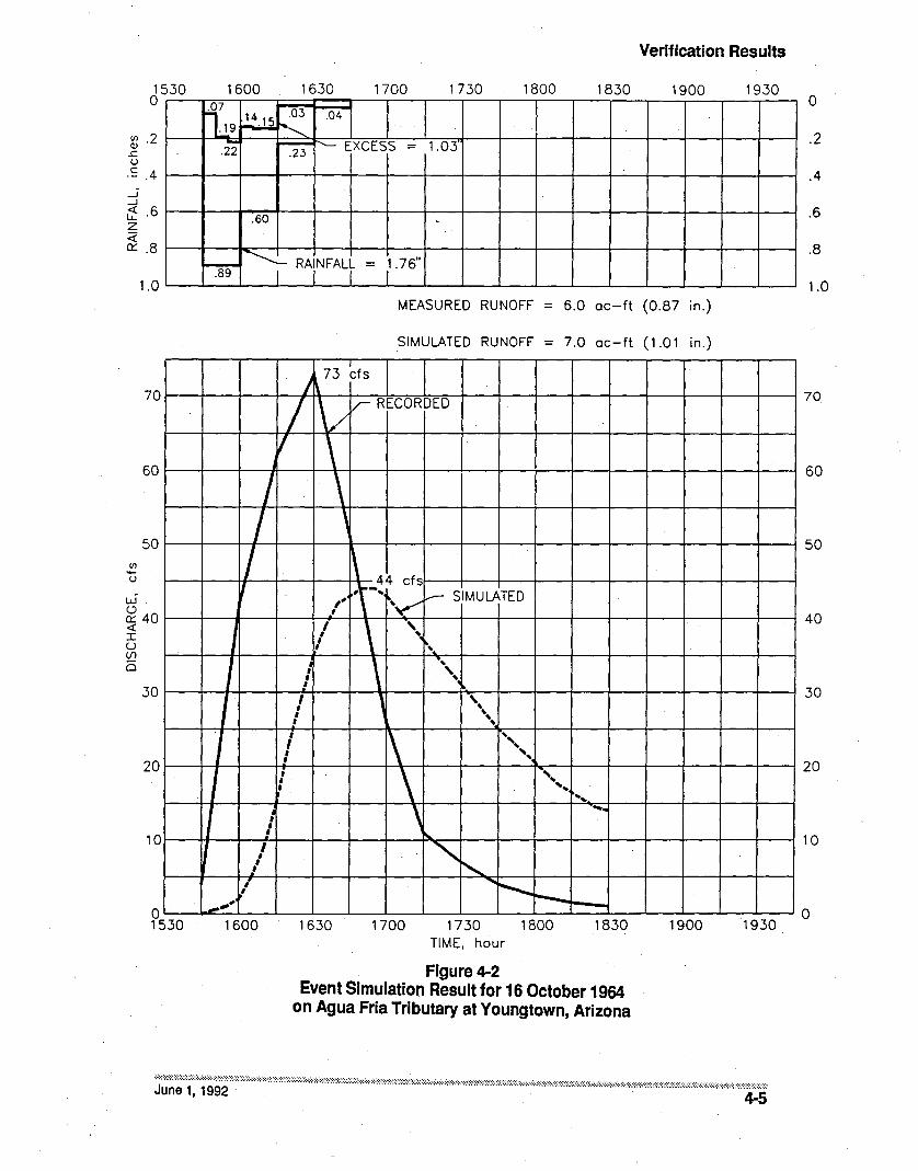
Verification Results
o19301900183018001730170016301600
1 .0314. 15.04
.19 - ..............- - EXCESS - 1.03.22 .23
.60
7 T RA\NFALr = 1 76"I'
1530o
~ .2 .2.!:u.~ .4 .4
1.0 1.0MEASURED RUNOFF = 6.0 ac-ft (0.87 in.)
-l-l
Ii .6 ;6z~~ .8 .8
SIMULATED RUNOFF = 7.0 ac-ft (1.01 in.)
30
h.73 cfs
70 ~-+---I--t--I-/-HI\r--~-+lr-r::'RE!=-;C"'O:-;:::R:kD-;:::;ED~--+--+---t---t--r--+--t--r---l70
1/ \60 I---.j--~/Jj.-+-\-\.j--.j--.j--+---+--.j--f---f---.j--.j--.j--+----l 60
/ 'III 50 I----l--+-I-/-+--+---l--~_+-_+-__+_-_+_-+_-f___+-_+-__+_-_+___j50
U ~---1f----+-I--+---l---H~1- 44 cfs;I----I--~--+---l--_+-_+_-_+_-_+_-+____iw IJ /' ,t-.. ~........... I-- SIMULATED
~ 40 1---If_-I--I--_++_I_-\-\-f-V'"~-+--4---f--I--__+-_+--l---+--+--+----l40
~ 1\'~ I ~
i5 i \ ~,~30 1----I-H--+~,4--+_--\+-,-_+_--h-,-f___+--+---+--+--+_-I---+----1
i 1 ~~~~
....\I•10l--~_I__-I---!-~.~-+__-.jl__-I------P~_+-_I_-__l_-+_--I--+----.;f___+-_+-_j 10
/ ,,~! I ........
20 1----+-I--+_ __+....i-~--If_-+i\--\-,__+-__l_-_+ .._,..-'_4.. 'r---+---l---+---+--_+_-_+_~ 20
! \ ~'"""
l ~""""""'I'--.-",' ---""'---'OL----J,~:........L..--L-...l--l---.J--.l.--.l...-....L-...L..--.L.----I---l..---L-.....L--...1.---l0
1530 1600 1630 1700 1730 1800 1830 1900 1930TIME. hour
Figure 4-2Event Simulation Result for 16 October 1964
on Agua Fria Tributary at Youngtown, Arizona

.05 0.0 0.0 0.0 I'""--
~ 0.0 0.0 0.0~.06 .07 I-
~ /I EXCESS .06 .01 .01 .01~ ~ .03 ~ .03.05 .05 .05
r-- .05 ...Jl- .15 .15I.11 I-- F-- .16 -
~ .21 ~ .20.25 .25 - .25 ~
"-I--
.30
I'\- RAINFALL ~
.45I--
I~ IRECOIRDED40.5 cfs
... - ... -
j "<V
Vl\?l.~!S V- SIMULATEDI
V~.. '\ ....('...
II
"....
~........."
..... ---- ~../ " " [::/"'- "'~""
" r----.... ..... ......,
/ '"V I
1\..
/ '" "..........-- "
,V 10'" \ .. ....
I .--- ...." r-.......
/ .' ,~
.................... ...............
V..................
MEASURED RUNOFF = 8.3 ac-ft (1.20 in.)5
.4
.3
30
2C
.2
40
10
2130o
o2130
2100
2100
2030
20302000
2000
1930
1930
1900
19001830
1830TIME. hour
1800
1800
1730
1730
1700
1700
1630
1630
1600
1600
SIMULATED RUNOFF = 9.0 ac-ft (1.30 in.)
Ul
u 30
o1530
.5
10
40
1530o
wC>0:::«I
~ 20o
~ .1r.u
S .2...J...J
~ .3z<C'0::: .4
~I
-------------------

Verification Results
;.::J.::IIII:I Academy Acres at Albuquerque, New Mexico
:1!!!!:.::I:!I!:I!·:·!!!II·!!~ The drainage area is a small (0.12 square mile) residential area developed' on an............... alluvial fan in the Northeast Heights of Albuquerque, New Mexico. Streets are the
major conveyance for storm runoff. There is a relatively short, concrete-linedchannel at the outlet of the watershed and the streamgage is located in the channel.The area consists of 191 single-family and 44 duplex residential units with a densityof about five units per acre. A church and paved parking lot are contained in theupper part of the watershed. The residences are generally landscaped with irrigatedlawns with a small amount of native vegetation that occasionally may be in gravelunderlain by plastic.
Streamflow recordS are available for 1978through 1983. A graphical flood frequencyanalysis was performed using the Cunnane plotting position equation and lognormal probability paper. A straight line was fit to the data and flood peakdischarges were estimated for return periods of 10-, 25- and 1OO-year.
Rainfall for the frequency simulation was developed by procedures in the HydrologyManual using rainfall statistics for this location from the NOAA Atlas for New Mexico(Miller and others, 1973b). For a watershed of this size-O.12 square miles-PatternNo.1 and a depth-area reduction factor of 1.0 were required.
Rainfall losses were calculated by the Green and Ampt infiltration equation andsurface retention loss. The soil is a sandy loam and the Green and Ampt parametersare: hydraulicconductivity (XKSAT) of 0.40 inch/hour, capillary suction (PSIF) of4.3 inches, and soil moisture deficit (DTHETA) of 0.25. The surface retention (IA)was estimated as 0.20 inch, and the effective impervious area (RTIMP) as 28 percent.
A single-basin model using the Clark unit hydrograph was developed. The unithydrograph parameters were calculated based on an area (A) of 0.124 square miles,watercourse length (L) of 0.9 mile, slope of 105 feet/mile, and resistance coefficientof 0.028. Tc and R varied for each flood return period since the procedures toestimate these parameters are a function of rainfall excess intensity, which variesfor each flood return period. The synthetic urban time-area relation was used.
The results of the graphical flood frequency analysis and results of the frequencysimulation are shown in Table 4-2 and Figure 4-4. The record length is only 14 years,
Table 4-2Results of Frequency Simulation for
Academy Acres at Albuquerque, New Mexico
Peak Discharge, cisRetum Period,
years
1025
100
Flood Frequency FrequencyAnalysis Simulation
95 92
130 133190 197
June 1,1992 4-7

- • Frequency Analysis-
<!) HEC-1 Flood Frequency Resul ts-
Return Period. yrs Qp, cfs-
-- 10 92
- 25 133100 197
-
~
~
/)~
",,""" •,
j"
•
•
1.25 2 3 5RETURN PERIOD. years
Figure 4-4Flood Frequency Analysis and Model Results
for Academy Acres at Albuquerque, New Mexico
DocumentationNerification Report I,-
"8 I7
6
5 I4
3 I2
II
1 I98
7 I6
5 I4
3 I2 I
I1 I98
7
I6
IIII
10050
25 50 100
2510
10
5321.25
1.01
1.01
4
3
5w()0::: 4«Iu~ 3o
2
5
2
(/) 6....u
10 1
98
7
6
100 198
7
1000
"87
6

Verification Results
11.·.1111111Iill:l1111
1:1:11: The drainage area is an 8.12 square mile mixed residential, commercial/industrial........... area that is drained by Tucson Arroyo. Defined and, in some cases, improved
drainage channels exist throughout the drainage area. The area consists of mostlyresidential units of four to five units per acre, with lawn and native vegetation.. Agolf course and several regional parks exist in the area comprising a total of aboutone square mile. A large railroad yard and associated industrial complex is includedthat occupies about one square mile. Regional commercial properties exist throughout the area.
Both frequency and event simulations were performed for this watershed. Severalmodels were developed for the watershed and these were single-basin modelsusingboth the Clark Unit Hydrograph and 5-graphs, and a multi-basin model using theOark Unit Hydrograph.
Streamflowrecords are available for 1956through 1981. A graphical flood frequencyanalysis was performed using the Cunnane plotting position equation and log-extreme value probability paper. A straight line was fit to the data and flood peakdischarges were estimated for return periods of 2- to 100-year.
Rainfall for the frequency simulation was developed by procedures in the HydrologyManual. A watershed of this size-8.12square miles-required Pattern No. 2.61 anda depth-area reduction factor of 0.95.
Rainfall losses were calculated by the Green and Ampt infiltration equation andsurface retention loss. The Green and Ampt parameters were area-averaged withhydraulic conductivity (XKSAT) of 0.26 inch/hour, capillary suction (PSIF) of 4.3inches, and soil moisture deficit (DTHETA) of 0.25. The surface retention (IA) wasestimated as 0.20 inch, and the effective impervious area (RTIMP) as 20.2 percent.
The watershed characteristics that were used to calculate the Oark Uirlt Hydrograph parameters Tc and R and the 5-graph Lag are shown in Table 4-3. Thesynthetic urban time-area relation was used with the Oark Unit Hydrograph.
The results of the graphical flood frequency analysis and results of the frequencysimulations by the various models are shown in Table 4-4 and Figure 4-5.
The record length is 26 years, therefore, greater emphasis should be placed incomparing flood peak discharges in the 2- to 5O-year return period range, althoughthere is closest agreement at the 10o-year flood leveL All of the models seem toadequately represent the flood frequency results, although the Oark Unit Hydrograph seems to be superior to 5-graphs for this urban watershed.
June 1,1992 4-9

DocumentationNerification Report
Peak Discharge, cIs
Frequency Simulations
Flood Multi-basinReturn Period, Frequency Single-basin Models Model
years Analysis Clark S-Graph Clark
2 800 1,130 1,400 1,2105 1,460 2,240 2,650 -
10 2,200 3,180 3,920 -25 3,600 4,790 5,870 5,26050 5,300 6,260 7,580 -
100 7,600 7,520 9,670 7,770
Area,A, Centroid Slope,square Length L, Length, S, Resistance Coefficients
mile miles Lea, miles foot/mile KbClark Kns-Graph
Single-Basin Model
8.12 6.18 2.7 37.7 0.0168 0.015 (tOO-year)0.019 (50-year)0.022 (25-year)0.026 (to-year)0.030 (5- & 2-vear)
Subbasin Multi-Basin Model
1 3.16 4.20 - 35.7 0.0193 -2 1.25 3.13 - 38.3 0.0219 -3 2.28 - 2.71 - 43.5 0.0202 -4 1.43 2.90 - 43.1 0.0215 -
IIIIIIIIIIIIIIIIIII
Rainfall and peak discharge data are available for 12 August 1972 to perform anevent simulation for this watershed. Rainfall data are available for 12 recordingraingages and six non-recording raingages in the watershed that are operated by
Table 4-4Results of frequency simulation for the Tucson Arroyo at Tucson
June 1, 1992
Table 4·3Watershed Characteristics used in Calculating
Unit Hydrograph Parameters for Tucson Arroyo
Both the Clark single-basin and the Clarkmulti-basin models yield similar resultsindicating that the Clark Unit Hydrograph procedure can beapplied to watershedslarger than the recommended 5 square mile criteria.
The 5-graph resistance coefficient (Kn> was increased for floods of magnitudesmaller than the 100-year flood. This was done to account for the lower hydraulicefficiency of runoff for the smaller events.
4-10

1.01 1.1 1.2 1.3 1.4 1.~ 3 6 7 8 9 10 20 30 40 ~O 100
3
100 I9
::!J 8
0_0
600.~"T1
~-1""'1eCD~.g 4
OCD (J)
:::J:::J -:t-"
U 3
~'< w~»"T1O:::J _. c:>'<m CC 0::: 2o _ e «m~ ; I
""-- u-Ien~ (f)
emU1 (5"~en a. 10 Ig=: 9- 0 8:t-o.::I. CD 7
N-60 :a
:::J CD~m enc
;:::; 4en
2
• Frequency Analysis- ® Clark, Single basin
&:. Clark. Multi basin
* S graph, Single basin
I
I - I I - I
~ -
3
1 1009
6
7
6
3
1 109
6
~
3~::I.-s·-0':::J:aCD(I)e
1 1 ;:::;(I)
1.01 1.1 1.2 1.3 1.4 1.~ 3 ~ 6 7 6 9 10 20 JO 40 :lO 100
RETURN PERIOD. years

DocumentationNerification Report
~12
the University of Arizona. For the 18 raingages in the watershed, the maximumrainfall depth is 1.93 inches, the minimum is 0.65 inch, and the average is 1.41 inch(0.36 inch standard deviation). The rainfall mass diagrams were plotted for eachrecording raingage and several rainfall distributions were prepared for the subbasins of the watershed. The peak discharge for the event (2,950 cfs) was recorded bythe USGS. Hydrograph data are not available for this event.
Two models were used for the event simulation: theClarksingle-basinand the Oarkmulti-basin models as previously described for the frequency simulations. For thesingle-basin model, the rainfall depth from a composite rainfall mass diagram is1.46 inches. For the multi-basin model, four rainfall mass diagrams were generatedfor use with each of the four subbasins. The rainfall depths for each subbasin are,1.23 inches for subbasin 1, 1.63 inches for subbasin 3, and 1.46 inches for subbasins2 and 4.
Frequency simulation was performed for each watershed, and an event simulationwas performed using data for watershed 63.011. Several different models weredeveloped for these watersheds using both the Clark unit hydrographand5-graphs.
Streamflow records are available for 1963 through 1989 for both watersheds.Graphical flood frequency analyses were performed using the Cunnane plottingposition equation and log-normal probability paper. A straight line was fit to thedata on each graph and flood peak discharges were estimated for return periods of10-, 25- and 100-year.
The models were ron using two different sources for rainfall statistics: the NOAAAtlas for Arizona (Miller and others, 1973a) and site-specific rainfall statistics as
June 1, 1992
IIIIIIIIIIIIIIIIIII

Verification Results
developed from information in Osborn and Renard (1988). There is considerabledifference between the rainfall statistics from these two sources. The site-specificrainfall statistics are appreciably higher than the NOAA Atlas statistics. For example, the NOAA loo-year, I-hour rainfall is 2.43 inches and the site-specific lOO-year,I-hour rainfall is 3.07 inches (a 26 percent increase over the NOAA statistic). Osbornand Renard do not provide rainfall depth-duration-frequency statistics for durations in excess of 1 hour. However, the Maricopa County procedure requires a6-hour rainfall depth to define the design storm. Therefore, the Osborn and Renardrainfall statistics were plotted on graph paper along with the NOAA statistics andthe Osborn and Renard statistics were extended to 6 hours to follow the same slopeof the NOAA lines. This graph was used to estimate the design 6-hour rninfall depthfor these watersheds. This mayor may not represent severe storms for the watershed. According to Osborn (personal communication, October 1991) the peakdischarges on both watersheds 63.011 and 63.008 resulted from rains of durationsless than 1 hour. Although 6-hour type storms may occur over the Walnut Gulchwatershed that have similar characteristics to the Maricopa County design stonn(1954 Queen Creek storm), such storms apparently have not occurred in that areasince the watershed was instrumented. Therefore, modeling of the Walnut Gulchwatersheds using the 6-hour Maricopa County design storm may not be representative of the appropriate regional meteorologic conditions. Nonetheless, modeling of these watersheds was performed using 6-hour rainfall depths as described.For watershed 63.011 (3.18 square mile) this required Pattern No. 2.07 and adepth-area reduction factor of 0.97, and for watershed 63.008 (5.98 square mile) thePattern No. is 2.44 and the depth-area reduction factor is 0.96.
Rainfall losses were calculated by the Green and Ampt infiltration equation andsurface retention loss. Watershed 63.011 is a subbasin of 63.008 and the same rainfallloss parameters were calculated for both watersheds. The Green and Ampt parameters were area-averaged with hydraulic conductivity (XKSAT) of 0.22 inch/hourafter correction for the 30 percent vegetation cover, capillary suction (PSIF) of 5.8inches, and soil moisture deficit (DTHETA) of0.39. The surface retention (IA) wasestimated as 0.35 inch, and the impervious area (RTIMP) as 0 percent
These two watersheds were modeledusing both the Clark unit hydrograph and thePhoenix Valley 5-graph. Watershed 63.008 was modeled as a single-basin and alsoas a two subbasin model. The watershed characteristics that were used to calculatethe Clark unit hydrograph parameters, Tc and R, and the 5-graph Lag are shown inTable 4-5. The synthetic natural time-area relation was used with the Clark unithydrograph.
The model results for the two watersheds using the two different rainfall input andthe various models are shown inTables 4-6 and 4-7. Those results indicate that peakdischarges using the NOAA rainfall statistics are considerably less than the floodfrequency estimates. Since the site-specific rainfall statistics more accurately reflectthe actual rainfall regime than do the NOAA Atlas statistics, it seems appropriateto evaluate· the model performance based on the site-specific rainfall statistics.Because of this, all results that are discussed are those using the site-specific rainfallstatistics that were developed from Osborn and Renard (1988).
June 1, 1992 4-13

DocumentationNerification Report
Peak Discharge. cfs
Return Flood Frequency SimulationPeriod. Frequency Using NOAA Statistics Using Site-5pecific Statisticsyears Analysis Clark u-hg 5-Graph Clark u-hg 5-Graph
10 .1,950 560 960 1,760 2,05025 2,950 1,170 1,570 2,030 2,290
100 6,500 2,300 2,500 4,380 4,190
Peak Discharge. cfs
Frequency SimulationReturn Flood Using NOAA Statistics Using Slte-5peclfic StatisticsPeriod. Frequency Clark Multi- Clark Multi-years Analysis u-hg 5-Graph Basin u-hg 5-Graph Basin
10 2,100 780 1,()60 920 1,790 2,450 2,07025 3,300 1,330 1,830 1,540 2,010 2,750 2,320
100 6,200 2,220 3,030 2,450 3,820 5,250 5,190
IIIIIIIIIIIj
IIIIIII
June 1,1992
Table 4-6Results of frequency simulation for the Walnut Gulch 63.011 watershed
Table 4-7Results of frequency simulation for the Walnut Gulch 63.008 watershed
Table 4-5Watershed characteristics used in calculating unit hydrograph parameters
for Walnut Gulch watersheds 63.011 ami 63.006centroid Resistance Coefficients
Area. Length. Length. Slope.~ L, Lea. S, Kb Kn
square mile miles miles feetlmile Clark s-Graph
Watershed 63.011 Single-Basin Model
3.18 4.0 1.8 100 0.033 0.03Watershed 63.008 Single-Basin Model
5.98 8.0 3.6 75 0.033 0.03Watershed 63.008 Multi-Basin Model (Clark only)
3.18 4.0 - 100 0.033 -2.80 4.0 - 75 0.033 -
4-14

Verification Results
Watershed 63.011 is smaller than the recommended 5 square mile upper limit forapplication of the Clark unit hydrograph, and, therefore, this watershed wasmodeled as a single basin. Model results for watershed 63.011 are shown in Table4-6 and Figure 4-6. The model results using both the Clark unit hydrograph and the5-graph are very close to the best estimate of the 10-year flood peak discharge. Theresults are not as good at the 25- and 10o-year return periods. Considering that thiswatershed is outside of Maricopa County and that the design rainfall criteria thatwere applied may not be completely representative of the regional severe stormcharacteristics, the results are reasonable.
Watershed 63.008 is a little larger than the recommended 5 square mile upper limitfor application of the Clark unit hydrograph, but is smaller than the absolute 10square mile upper limit for application. Therefore, this watershed was modeled asa single basin using the Clark unit hydrograph and the 5-graph, and was alsomodeled as a multi-basin (two subbasins) watershed using the Oark unit hydrograph. When modeled as a single basin, the calculated Tc (1.5 hour) exceededthe duration of rainfall excess (1.0 hour) indicating that this watershed should notbe modeled as a single basin when using the Clark unit hydrograph procedure asdescribed in the Hydrology Manual.
The model results, shown in Table 4-7 and Figure 4-7, are not particularly goodwhen the watershed is treated as a single basin with the Clark unit hydrograph.This provides evidence that the size recommendations for the Clark unit hydrograph procedure should not be exceeded if the calculated Tc exceeds theduration of rainfall excess.
The results of the single basin, 5-graph model are reasonable. This indicates that,for small desert rangeland watersheds, the Phoenix Valley 5-graph is a viable unithydrograph procedure and it can be used in certain applications where the Clarkunit hydrograph is either inappropriate (exceeds size limitations) or where expedience may warrant the use of an 5-graph rather than the Clark unit hydrograph.
The multi-basin, Clark unit hydrograph model yielded reasonable results for thefull range of return periods. This indicates that the Clarkunit hydrograph can beused for l~ger watersheds where it is either necessary or desirable to model thewatershed as a system of subbasins.
The model results for both watersheds 63.011 and 63.008 are highly dependent uponthe ability of the rainfall input to reflect local, severe storm rainfall characteristics.The rainfall criteria that were applied to these watersheds was developed from anhistoric ,7-hour duration local storm in Maricopa County as represented by the6-hour design rainfall criteria in the Hydrology Manual. That rainfall may not berepresentative of the spatial and temporal distributions of rainfall that actuallyoccur in the Tombstone area. Therefore, the accuracy of the developed rninfall-runoff models to reproduce a recorded flood frequency relation must be interpretedwithin this assumption.
Rainfall and mnoff data are available for watershed 63.011 for 4 August 1980 toperform an event simulation for this watershed. Rainfall data are available for ninerecording rningages in the watershed. For the nine rningages, the maximum rainfall
June 1,1992 4-15

DocumentationNerification Report
-• Frequency Analysis
-HEC 1 Flood Frequency Results-
Unit Hydrograph Rain-
-S Graph Site Specific- (!)
- 0 Clark Site Specific[!J S Graph NOM
- & Clark NOM
~ t~
•
10,0009
8
7
6
5
4
3
2
1000 1
98
7
V1 6....u
5wC)~ 4«Iu~ 3o
2
100 1
98
7
6
1.01 1.25 2 5 10 25 50 100
1.01 1.25 2 3 . 5RETURN PERIOD, years
10 25 50 100
Figure 4-6Flood Frequency Analysis and Model Results for Walnut Gulch 63.011

Verification Results
-• Frequency Analysis.
-HEC 1 Flood Frequency Results
-RainUnit Hydrograph
-
Single Basin Models-
S Graph Site Specific- @
0 Clark Site Specific-.0 S Graph NOAA
- &. Clark NOAA- Multi Basin Models
- • Clark Site Specific)( Clark NOAA
.,II
10,0009
8
7
6
5
4
3
2
1000 19
8
7
(f) 6.....u
5wC)n::: 4<l:IU<;0 3o
2
100 1
98
7
6
1.01 1.25 2 :3 5 10 25 50 100
98
7
6
5
4
3
2
198
7
6
5
4
3
2
198
7
6
1.01 1.25 2:3RETURN PERIOD, years
5 10 25 50 100
Figure 4-7Flood Frequency Analysis and Model Results for Walnut Gulch 63.008

DocumentationNerification Report
4-18
depth is 1.89 inches, the minimum is 0.72 inch, and the average is 1.26 inches (0.44inch standard deviation). Thiessen polygons of the raingage network were prepared, rainfall mass diagrams were plotted for each raingage, and representativerainfall distributions were selected for the subbasins of the watershed.
An eight subbasin model of the watershed was developed to represent the arealdistribution of rainfall. The rainfall loss parameters were the same for each subbasinand the parameter values were equal to the values for the watershed as previouslyreported. The Phoenix Valley S-graph was used because the duration of rainfallexcess for some of the subbasins was too short to use the Qark unit hydrographprocedure.
The model, with input as described, resulted in a runoff of about 44 acre-feet with,a peak discharge of 886 cis at time 14:05. The recorded runoff was about 30 acre-feetwith a peak discharge of 894 ds at time 13:47. The recorded and simulated hydrographs are shown in Figure 4-8.
The simulated peak discharge very accurately represents the recorded peak. Therunoff volume is overestimated. However, this can be at least partially accountedfor by two factors that are not incorporated in the model. First, the watershed hastwo stock ponds, neither ofwhich was modeled. The upper stockpond has virtuallyno recorded or modeled runoff therefore it does not contribute to the error. Theother stock pond is near the center of ,the watershed and that pond may haveretained some of the runoff volume, thereby leading to model overestimation.Second, channel· transmission losses are not included in the model. Estimation oftransmission losses would reduce runoff volume from the model. Although transmission losses can. significantly reduce runoff volumes, the peak discharge isusually only slightly reduced for small, high intensity storms such as this. Therefore,the runoff volume would be reduced from the 44 acre-feet estimate, but the peak of886 ds would be only moderately reduced.
June 1, 1992
IIIIIII,IIII'IIIIIIII

Verification Results
a 50 100 150 200 250
25020015010050
flllflflt I/ltl//II Iltlltltl 1f1!1I111 II I II ) J I I " I I I I
894 cfs 886 cfs
" •1\·,••• MEASURED RUNOFF = 30 ac-ft• •• •• • .• • SIMULATED RUNOFF 44 ac-ft• • =: !
• •RECORDED ----....... • V SIMULATED•••: •• •• •• !
• •• •I I
• •II ••• •• \•: •I• •I •• •
I i• •I
!•••!\
I •• !
• ••• •: ••; i, •! \t ••• ,• •, ,I
r~i
• \: \• V \ \•I \• ,• ,i \
-'..• '..• "!• '---
..• "•: ' ...._-II I I I I 1 I I I I 1 I I I 111 1111 11 I 1 I I I T I I j I f1 I I I I I I I I I II I I I Io
o
100
900
700
800
200
300
1000
600(f).....u
w<.:>
50000::<!IU(f)
0
400
TIME. minutes
Figure 4-8Event simulation results for 4 August 1980 onWalnut Gulch 63.011 near Tombstone, Arizona
June 1, 1992 4-19

DocumentationNerification Report
III Cave Creek
Area-averaged rainfall loss parameters calculated by the Green and Ampt infiltration equation for the five subbasins are shown in Table 4-8.
The Phoenix Mountain 5-graph was used to develop the unit hydrographs for thesubbasins. The watershed characteristics, resistance coefficients, and calculatedLags for the subbasins are shown in Table 4-9.
IIIII\1IIIt·IIIIIIIII
June 1,1992
Table 4-8Rainfall Loss Parameters for the Cave Creek Model
The resultsof the graphical flood frequency analysis and the frequency simulationare shown in Table 4-10 and Figure 4-9. The record length is 26 years, therefore,greater emphasis should be placed in comparing flood peak discharges in the 2- toSO-year return period range, although the frequency simulation results are the bestfor the lOO-year flood. The 2-year flood peak is overestimated and this is probablybecause the more frequent floods are caused by partial area rainfalls that do notcover the entire watershed, and because channel transmission losses are not incorporated in the model and such losses are more significant for the smaller rainfalls.
!li:i!i!·illjl!i·l··:i~i·i!I:! The 127 square mile watershed is composed of hilly Sonoran desert and ruggedmountain. The elevation range is from about 1,900 feet to about 5,100 feet.Vegetation is sparse, consisting mainly of cacti and rangeland grasses and forbs. Considerable rock outcrop occurs throughout the watershed although the outcrop is notdirectly connected to the outlet.
Streamflow records areavailable for 1958 through 1989. A graphical flood. frequencyanalysis was performed using the Cunnane plotting position equation and extremevalue probability paper. A straight line was fit to the data and flood. peak dischargeswere estimated for return periods of 2- to lOO-year.
A multi-basin model was developed Using five subbasins. Rainfall for the frequencysimulation was developed by procedures in the Hydrology Manual. A watershed ofthis size-127 square miles-required Pattern No. 4.2 and a depth-area reductionfactor of 0.78.
Hydraulic capillary Soli SUrface ImperviousConductivity, SUction, Moisture Retention, Area,
XKSAT, PSIF, Deficit, lA, RTIMP,SUbbasin inch/hour inches DTHETA inches %
A 0.28 4.8 0.35 0.25 26B 0.38 4.2 0.35 0.25 10C 0.30 4.7 0.35 0.25 190 0.26 4.9 0.35 0.25 6E. 0.25 3.5 0.35 0.25 0
4-20

Verification Results
Table 4·9Watershed Characteristics and S-graph Parameters for the Cave Creek Model
Area, Length, centroidA, L, Length, Slope,S,
SUbbasin square mile miles Lea, miles feetlmile Kn Lag, hoursA 80.28 22.0 15.0 105 0.045 4.05B 34.86 9.33 5.67 152 0.05 2.09C 6.38 6.33 3.41 95 0.05 1.620 4.81 8.33 5.05 120 0.05 2.00E 0.59 2.84 0.95 83 0.05 0.76
Table 4-10Results of Frequency Simulation for Cave Creek at cave Creek .
Peak Discharge, cfsReturn Period,
years
2
5102550
100
Flood FrequencyAnalysis
1,3004,8007,000
10,00012,40014,600
Simulation
3,4004,4006,0009,100
11,80014,600
June 1, 1992 4-21

IIIIIIII'IIII.JJI(1\
I~
II
10 (f)'+-u
000
c8
W<..:l0::::«:r:u(f)
06
12
4
14
2
June 1, 1992
RETURN PERIOD IN YEARS
25 50 10016
o25 50 100
RETURN PERIOD IN YEARS
10
10
5
532
Figure 4-9Flood Frequency Analysis and Model Results for
Cave Creek near Cave Creek, Arizona
/
/1/
//
/
//
/
•
v.
•
o
4-22
c8
12
2
® HEC-l Flood Frequency Results
• Frequency Analysis 2 316
14
4
6
DocumentationNerification Report
(f) 10'+uooo
W<..:l0::::«:r:u(f)
o

Verification Results
f1!t//?i\}:!.!::i:I!II·. Agua Fria River
il,j:jilii!j:lillillilil:jil:!· The 588 square-mile watershed is mountainous with an elevation range from about3,400 feet to about 7,000 feet. The watershed is composed of conifer forest, openrangeland, and high elevation desert.
Streamflow records are available for 1940 through 1989. A graphical flood frequencyanalysis was performed using the Cunnane plotting position equation and log-normal probability paper. A straight line was fit to the data and flood peak dischargeswere estimated for return periods of 2- to 10o-year. The flood frequency graph isshown in Figure 4-10.
A multi-basin model was developed using 11 subbasins. Because of the size of thewatershed, three different rainfall criteria, as summarized below, were used tosimulate both local storms and general storms. Rainfall depth-duration-frequencystatistics were developed using NOAA Atlas 2 and Arkell and Richards (1986) forthe three rainfall criteria.
Rainfall Distribution
Maricopa CountySCS Type IIHypothetical
Rainfall Duration Depth-Area Reduction
~hour Maricopa County Manual24-hour NWS HYDR0-40 (Zehr and Myers, 1984)24-hour NWS HYDR0-40 (Zehr and Myers, 1984)
Area-averaged rainfall loss parameters calculated by the Green and Ampt infiltration equation for the 11 subbasins are shown in Table 4-11.
Five ~graphs from the ~raphReport (Sabol, 1987) were evaluated for use on thiswatershed: the Phoenix Mountain, the Agua Fria River (general storm), the AguaFria river (local storm), the Average for Arizona, and the Average Mountain. Thetwo Agua Fria River~graphs are probably the most appropriate for this watershed,however, because they are so similar to the Phoenix Mountain ~graphand becausethe Phoenix Mountain and the Agua Fria River ~graphs produce about the sameresults, the Phoenix Mountain ~graph was selected for use with all subbasins ofthe model. The watershed characteristics, resistance coefficients, and calculated.Lags for the subbasins are shown in Table 4-12. A resistance coefficient <Kn> of 0.043was used for all subbasins for a 6-hour storm and 0.059 for a 24-hour storm.
Since this watershed. has a 5O-year period of record and assuming a Binomialdistribution for the occurrence of floods, there is a 64 percent probability that aSO-year flood event occurred. during the period of record. Therefore, the projectionof the flood frequency line to a 100-year return period should result in a fairlyreliable estimate of the 100-year flood peak discharge. For watersheds of this size,it is unlikely that there will be a practical need to estimate flood magnitudes forreturn periods less than lOO-year; therefore, the various models were only comparedto the graphical flood frequency analysis results at the lOo-year return period value.
June 1, 1992 4-23

Figure 4-10Flood Frequency Analysis for Agua Fria River near Mayer, Arizona
• Frequency Analysis
DocumentationNerification Report II
100 I98
7 I6
5
I4
3 I2 I
I1 109 I8 en7u
6 0
I00
5~
c
4 •
Iw'-'~
34:IU
'I(f)
is
2
I1 1 I98
7 I6
tIII
June 1, 1992
RETURN PERIOD IN YEARS5 10 25 50 100
5 10 25 50 100RETURN PERIOD IN YEARS
3
3
2
2
II
l.I
/'/'
M
3
4
1 198
7
6
2
2
10 198en
U 7
g 6o~ 5c
• 4w'-'~
:2 3u(f)
o
10098
7
6
5

Verification Results
Table 4-11 ;Rainfall Loss Parameters for the Agua Fria River Model
Hydraulic Capillary Soil SUrface ImperviousConductivity, SUction, Moisture Retention, Area,
XKSAT, PSIF, Deficit, lA, RTIMP,SUbbasin Inchelhour Inches DTHETA Inches %
1 0.25 5.0 0.35 0.25 5.5
2 0.29 4.7 0.35 0.25 8.0
3 0.33 4.5 0.35 0.25 8.5
4 0.31 4.6 0.35 0.25 7.5
5 0.28 4.8 0.35 0.25 10.0
6 0.11 6.9 0.36 0.25 10.0
7 0.09 7.5 0.33 0.25 6.38 0.05 9.0 0.27 0.25 6.5
9 0.10 7.2 0.35 0.25 4.3
10 0.06 8.6 0.29 0.25 8.0
11 0.34 4.4 0.35 0.25 9.0
Table 4-12Watershed Characteristics and S-graph Parameters
for the Agua Fria River Model
Area,A, Length, centroid Slope, Lag, hourssquare L, Length, S, 6-hour 24-hour
Subbasin miles miles Lea, miles feet/mile storm storm
1 37.8 9.67 4.33 175 1.60 2.202 85.4 18.15 10.26 142 2.93 4.02
3 80.3 17.56 9.47 113 2.93 4.024 46.1 14.20 6.51 155 2.21 3.035 44.6 15.59 8.68 167 2.52 3.466 30.6 8.29 3.95 97 1.63 2.247 61.9 14.20 8.68 84 2.77 3.808 58.5 12.11 7.89 198 2.14 2.949 13.0 5.52 2.25 47 1.29 1.77
10 65.6 17.36 11.84 161 2.97 4.0811 64.2 23.67 14.20 93 3.98 5.46
June 1, 1992 4-25

DocumentationNerification Report
The results of the model for the three rainfall criteria are:
The partial area rainfall results and the flood frequency analysis are interesting inthat they indicate that the observed floods for this watershed may be the result oflocal storms that occur over only parts of the watershed, rather than large generalstorms that cover the entire watershed. The results also indicate that the SCS TypeII distribution may result in unrealistically high peak discharges when the drainagearea is much larger than 100 square miles. The peak discharges for the hypotheticaldistribution are less than those for the Maricopa County distribution for areas lessthan about 250 square miles and are greater for areas larger than 250 square miles.
III1IIIIIIIIIIIIIIIJune 1, 1992
27,100 cfs72,800 cis45,600 cis
Table 4-13Partial Area Rainfall Results for the AQua Fria River
Maricopa County, 6-hourSCS Type II, 24-hourHypothetical, 24-hour
Compared with the flood frequency analysis (37,000 cfs), none of these results areparticularly attractive.
The model was used with rainfall over only selected subbasins to investigatewhether partial area rainfall from local storms over the watershed could be thedominant flood-producing event for this watershed. The three rainfall criteria thatwere input to the models were prepared for rainfall over selected portions of thewatershed. The results are shown in Table 4-13 and Figure 4-11.
The results in Figure "4-11 indicate that the 10o-year flood peak discharge is produced for partial area rainfall and the Maricopa County local storm rainfall criteriafor areas between about 175 to 250 square miles. For areas larger than this, the peakdischarge decreases as the local storm area increases. The other two rainfall criteriaproduce increasing flood peak discharges as the storm area increases. This type ofresponse is representative of a general storm over a watershed of this size.
Peak Discharge, cfsArea, Maricopa County SCS Type II Hypothetical
square mile 6-hour 2~our 2~our
13.0 7,000 6,700 5,90065.6 17,300 17,400 13,400
124.1 31,600 33,200 24,000199.0 37,800 46,300 31,300229.6 38,100 52,800 35,000274.2 36,000 56,200 36,700320.3 34,900 63,700 41,400400.6 30,500 67,500 42,400588.0 27,100 72,800 45,600
4-26 .

Verification Results
.... "", ........ ,...... ......",
, , --r--- TYPE-II.' SCS 24-HR.'.'.~...#••
~ HYPOTHETICAL 24-HR.' V,.. ..,
~.. ..... -"_..
,.,s- ••••• ~.-
......' ~199__ YL __Qp_____~ZJ.QQ9__~f~-- -- --- -- -- --~ --- -- E> -- -- ----~. .
...~ Ji-•••• r-.~~
V'. '\....
'".i/ .
"'- MARICOPA CO. 6-HR.'..,/ .'.'.'
/. .'..,(. ..'
100,000
90,000
80,000
70,000
60,000
2u
w 50,000C)0::<:I 40,000uVlCl
::<:: 30,000<{wCl.
20,000
10,000
aa 100 200 300 400 500 600
WATERSHED AREA, sq. miles
Figure 4-11Agua Fria River WatershedPartial Area Rainfall ResultsThree Rainfall Distributions
11
1111111111111 Summary of Verifications
:::::::::::::::::::::::::::::::
l:ifiilllii!I'lliiiliilli::lii Flood frequency simulation was performed for four watersheds in Arizona that
have streamgage records. Flood peak discharges were estimated using proceduresin the Hydrology Manual for three of the watersheds for a range of return periods of2- to 100-year, and for one of the watersheds for the loo-year return period flood.For the"three watersheds for which ranges of flood discharges were estimated, theratio of the flood peak discharge as estimated by the model to the discharge fromthe flood frequency analyses are shown in Table 4-14.
For the 588 square-mile Agua Fria River watershed, only the lOO-year flood peakdischarge was estimated by modeling procedures. The lOo-year flood peak dig.;
charge was reproduced for local storm partial area·rainfall over about 175 to 250square miles using procedures' in the Manual. Using the SCS Type IT rainfalldistribution over the entire watershed resulted in a ratio of flood peak discharge to

DocumentationNerification Report
Ratio of flood peak discharges estimated by proceduresIn the Hydrology Manual to discharges from
flood frequency analyses
Agua Frla
ReturnRiver Tucson Academy
Tributary at Arroyo at Acres at Walnut Gulch Walnut Gulch cave CreekPeriod, years Youngtown Tucson Albuquerque 63.011 63.008 at cave Creek
2 1.0 1.41 2.62
5 1.03 1.53 0.92
10 1.0 1.45 0.97 0.90 0.99 0.86
25 0.88 1.33 1.02 0.69 0.70 0.91
50 0.75 1.18 0.95
100 0.65 0.99 1.04 0.67 0.84 1.00
4·28
Table 4-14Results of verifications for the Agua Fria River Tributary,
Tucson Arroyo, Academy Acres, Walnut Gulch Watersheds, and Cave Creek
discharge from the flood frequency analysis of 1.97. Using a 24-hour hypotheticaldistribution over the entire watershed resulted in a ratio of flood peak discharge todischarge from the flood frequency analysis of 1.23.
For estimating flood peak discharges for large watersheds in Maricopa County, tworainfall criteria should be used: 1) a local storm criteria using the procedures in theHydrology Manual for partial area storms; and 2) a general storm criteria. Thehypothetical distribution with depth-area reduction by NWS HYDRO-40 appearsto be a reasonable general storm criteria for use in Maricopa County.
Only limited rainfall-runoff data are available for performing event simulations.The event simulations that were performed indicate that the rainfall loss procedureand the Clark Unit Hydrograph procedure from the Hydrology Manual providereasonable reproduction of the rainfall-runoff process in Arizona.
June 1,1992
IIIIIIIII'IIIIIIIIII

RellicesII:ij:ilj:i!i:iiij:jiii;i~iiiii·:·.:!iilli:iiiiillli!iiii:il
Abott, J., 1978, Testing of several runoff models on an urban watershed, Technical PaperNo. 59, The Hydrologic Engineering Center, U.S. Army Corps of Engineers,Davis, California, 43 p.
Arkell, RE., and Richards, F., 1986, Short duration rainfall relations for the westernUnited States: Conference on Climate and Water Management - A Critical Era,Ashville, N.C., published by American MeteorologicalSociety, Boston, MA.
Clark, C.O., 1945, "Storageand theunithydrograph," Trans. American SodetyofCivilEngineers, V. 110, pp. 1419-1488.
Cochran, B.J., Hodges, HE., Livingston, RK., and Jarrett, RD., 1979, Rainfall-runoffdata from small watersheds in Colorado, October 1974 through September 1977,U.S. Geological SUrvey Open-File Report 79-1261, Denver, Colorado, 673pgs.
Craig, G.S., and Rankl, J.G., 1977, Analysis of runoff from small drainage basins, U.S.Geological Survey Open-File Report 77-727, Cheyenne, Wyoming, 88 pgs.
Cudworth, A.G., 1989,Flood HydrologyManual, U.S. Bureau ofReclamation, Denver,Colorado, 243 p.
Ducret, G.L., and Hodges, HE., 1972, Rainfall-runoff data from small watersheds inColorado, June 1968 through September 1971, U.S. Geological Survey BasicData Release No. 27, Denver, Colorado, 300 pgs.
-, 1975, Rainfall-runoffdata from small watersheds in Colorado, October 1971 throughSeptember 1974, U.S. Geeological Survey Basic-Data Release No. 38, Denver,Colorado, 540 pgs.
Fischer, E.E., Rote, J.J., and Borland, J.P., 1984, Rainfall-runoffdata in the Albuquerque,New Mexico, metropolitan area: 1976-1983, U.S. Geological Survey Open-FileReport 84-448, Albuquerque, NM, 306 pgs.
:.;.:.:.;.:.;.;.;.;.;.:.;.;.;.:::.:.;.;.;.;.;.;.:.;.;.;.:.;.;.:.;.;.:.;.:.:.;.;.;.;.;.;.;.;.;.;.;.;.:.;.:.:.:.:.:.;.:.;.;.;.;.:.;.;.;.;.;.;.;.:.:.:.:.;.:.:.:.:.:.:.:.;.:.;.;.;.:.:.:.;.;.:.:-:.:.;.:.:.:.:.:.;.;.;.;.;.;.;.;.:.;.;.:.;.;.;.;.:.:.;.:.:.:.:.:.:.:.:.:.:.:.:.:.;.:.:.:.:.:-:.:.;.:.:.:.;.:.:.:-:.:.;.;.:.:.:.:.:.:.:.:.:.:.:.:.:.:.:-:.:.:.:.:-:.:.;.:.:.:-:.;.:.:.:.:-:.:.;.:.:.:.:.:.:.:.:.:-;.:.:.:.:.:.:.:.:.:.:.;.:.:.:.:.:.:.:.:.:.;.:.:.:.:.
June 1,1992 5·1

:.;.:.;.:.:.:.:.:.;.;.:.;.;.:.;.:.:.;.;.:.:.:.:.:.:.:.:.:.:.:.:.:.:.:.:.:.:.:.:.:.:.:.:.:.:.:.;.:.;.:.;.:.:.:.:.;.;.:.:.:.;.;.:.:.:.:.:.:.:.:.:.:.:.:.:.:.:.:.:.:.:.:.:.:.:.:-:.:.:.:.;.:.:.:.:.:.:.:.:.:.:.:.:.:.:.:.:.:.:.:.:.:.;.:.:.:.:.:.:-:.:.:.;.:.:.:.:.:.;.;.;.:.:.;.:.:.:.:.:.:.:.:.:.:.:.:.:.:.:.:.:.:.:.:.:.;.;.:-;.;.:.:.:.:.:.;.:.:.:.;.:.:.:.;.:.:.;.:.;.:.;.:.:.:.:.:.:.:.:-:.;.;.:.:.:.:-:.:.:.:.:-:.;.:.;.:.;.:.:.:.:-;.:.:.:.:.:.:.:.:.:-:.:.:-:
DocumentationNerificatlon Report
5·2
Gibbs, J.W., 1981, Hydrologic Data for urban storm runoff from nine sites in the Denvermetropolitan area, Colorado, U.S. Geological Survey Open-File Report 81-682,Denver, Colorado, 142 pgs.
Gibbs, J.W., and Doerfer, J.T., 1982, Hydrologic data for urban storm runoffin the Denvermetropolitan area, Colorado, u.s. Geological Survey Open-File Report 82-872,Denver, Colorado, 553 pgs.
Henderson, F.M., and Wooding, RA., 1964, "Overland flow and groundwater flowfrom a steady rainfall of finite duration," Journal of Geophysical Research, V.69, No.8, pp. 1531-1540.
,Kent, K.M., 1973, A method for estimating volume and rate of runoff in small watersheds,U.S. Department of Agriculture, Soil Conservation Service, Technical PaperNo. 149.
Loague, K, and Freeze, R, 1985, "A comparison of rainfall-runoff modeling techniques on small upland catechments," Water Resources Research, V. 21, No.2
Miller, J.F., Frederick, RH, and Tracey,R.J., 1973, NOAA Atlas 2, Precipitation-frequency atlas of the western United States, Volume VIII, Arizona, NationalWeather Service, U.S. Department of Commerce, Silver Springs, MD.
Moore, 1.0., 1981, ''Effect of surface sealing on infiltration," Trans. American SocietyofAgricultural Engineers, V. 24, p. 1546-1561.
Osborn, HB., 1983, Precipitation characteristics affecting hydrologic response of southwestern rangelands, U.S. Department of Agriculture, Science and EducationAdministration, ARM-W-34.
Osborn, HB., and Davis, D.R, 1977, "Simulation of summer rainfall occurrence inArizona and New Mexico, Hydrology and Water Resources in Arizona andthe Southwest," Arizona Academy of Sciences, Hydrology Section, Proceedings,V. 7, p. 153-162.
Osborn, H.B., and Hickok, RB., 1968, Variability of rainfall affecting runoff from asemiarid rangeland watershed, Water Resources Research, V. 4, No.1.
Osborn, HB., Lane, L.J., and Myers, V.A., 1980a, ''Rainfall/watershed relationshipsfor southwestern thunderstorms," Trans. American Society of AgriculturalEngineers, V. 23, No. I, p. 82-87, 91.
Osborn, HB., Shirley, ED., Davis, D.R, and Koehler, 1980b, Model of time and spacedistribution ofrainfall in Arizona and New Mexico, U.S. Department of Agriculture, Science and Education Admin., ARM-W-14, 27 p.
Osborn, HB., and Renard, KG., 1988, "Rainfall intensities for southeastern Arizona," American Society of Civil Engineers, Journal of Irrigation and Drainage,V. 114, No. I, p. 195-199.
June 1, 1992
IIIIIIIIIIII 'IIIIIII

References
Papadakis, CN., and Kazan, M.N., 1987, Time ofconcentration in small, rural watersheds: American Society of Civil Engineers, Proceedings of the EngineeringHydrology Symposium, Williamsburg, Virginia, pp. 633-638.
Ponce, V.M., 1991, 'The kinematic wave controversy" American Society of CivilEngineers, Journal ofHydraulic Engineering, V. 117, No.4, pp. 511-525.
Ragan, RM., and Durn, J.O., 1972, ''Kinematic wave nomograph for times ofconcentration," American Society of Civil Engineers, Journal of the HydraulicsDivision, V. 98, No. HYI0, pp. 1765-1771.
Rankl, J.G., and Barker, D.S., 1977, Rainfall and runoff data from small basins inWyoming, U.S. Geological Survey, Cheyenne, Wyoming, 195 p.
Rawls, W.J., and Brakensiek, D.L., 1983, "A procedure to predict Green and Amptinfiltration parameters," Proceedings of the American Society of AgriculturalEngineers Conference on Advances in Infiltration, Chicago, illinois, pp. 102-112
Rawls, W.J., and Brakensiek, D.L., and Miller, N., 1983, "Green-Ampt infiltrationparameters from soils data," American Society of Civil Engineers, Journal ofHydraulic Engineering, V. 109, No. I, pp. 62-71.
Rawls, W.J., and Brakensiek, D.L., and Savabi, M.R, 1989, ''Infiltration parametersfor rangeland soils," Journal ofRange Management, V. 42, No.2, pp. 139-142
Resnick, S.D., DeCook, KJ., and Phillips, RA., 1983, Hydrological and environmentalcontrols on water management in semiarid urban areas - Phase II, Water Resources Research Center, University of Arizona, Tucson, Arizona.
Sabol, G.V., 1987, S-Graph Study (report for the Flood Control District of MaricopaCounty), Phoenix, Arizona, 29 pp. plus appendices.
-, 1988, "Clark Unit Hydrograph and R-parameter estimation," American Societyof Civil Engineers, Journal of the Hydraulic Engineering, V. 114, No. I, pp..103-111.
Sellers, W.O., 1960, 'The climate in Arizona," in Arizona Climate, by CR. Green andW.O. Sellers, Univ. of Arizona Press, p. 5-64.
Tiptonand Kalmbach, Inc., 1986,Reviewofdesign rainfall criteria andevaluation ofraingagenetwork: Index No. ST-853143, City of Phoenix, Engineering Department,40 p.
U.S. Army Corps of Engineers, 1974, Gila River Basin, New River and Phoenix CityStreams, Arizona, Design Memorandum No.2, Hydrology, Part 1, Los AngelesDistrict.
--,1980, Whitewater River Basin, feasibility reportforflood control and allied purposes,San Bernardino and Riverside Counties, California, Los Angeles District.
:.:.:.:.;.:.:.:.:.:.:.:.:.:.:.:.:.:.:.;.;.;.:.:.:.:.:.;.:.:.:.:.:.:.:.:.:.:.:.:.:.:.:.:.:.:.:.:.:.:.:.;.;.:.;.;.:.;.:.:.:.:.:.:.:.:.:.:.;.;.:.;.:.:.;.:.:.:.;.:.:.:.:.:.:.:.:.:.;.;.:.:.:.:-:.:.:.:.:.:.:.:.:.:.:.;.:.:.:.:.:.;.;.:.:.:.:.:.:.:.:.:.:.:.:.:.;.:.:.:.:.:.:.:.:.:.;.;.:.;.;.;.:.;.:.:.:.:-:.:.:.:.:.:.:.:.:.:.:.:.:.:.:.:.:.:.:.:.:.:.:.;.;.:.:.:.;.:.:.;.;.:.;.;.;.;.:.:.:.;.:.:.:.:.;.:.:.:.:.:.;.:.:.:.:.:.;.;.:.:.:.;.:.:.;.:.:.;.;.:.:.:.:.:.:.
June 1,1992 5-3

IIIIIII
.1IIIIIIIIII
(i
IJune 1, 1992
Van Mullem, J.A., 1989, Applications of the Green-Ampt infiltration model to watershedsin Montana and Wyoming, thesis presented to Montana State University,Bozeman, 90 p.
__, 1982b, Hydrologic analysis of ungaged watersheds using HEC-l, HydrologicEngineering Center, Training Document No. 15, 122 p. plus appendices.
__, 1988a, Gila River and tributaries, Rillito River, Tucson, Arizona, General DesignMemorandum, Hydrology Appendix, Los Angeles District, 39 p.
--1988b, Hydrologic documentation for feasibility study, lAs Vegas Wash and tributaries, Clark County: Nevada, 242 p.
--, 1990, HEC-l Flood Hydrograph Package, Users Manual.
Zehr, RM., and Myers, V.A., 1984, Depth-area ratios in the semi-arid southwest UnitedStates: Technical Memorandum No. NWS HYDR0-40, National Oceanic andAtmospheric Administration.
u.s. Bureau of Reclamation, 1987, Design of Small Dams, Third Edition, Denver,Colorado, 860 p.
--, 1988, PREFRE, Computation of precipitation frequency-duration values in thewestern United States, Program Users Manual, Flood Section, Surface WaterBranch, Earth Sciences Division, Denver, Colorado.
__, 1982a, Gila River Basin, Phoenix, Arizona and vicinity (including New River),Design Memorandum No.2, Hydrology Part 2, Los Angeles District, 59 p.
5·4:.;.:.:.:.;.:.;.:.:.;.:.:.:-:.;.:.;.;.;.;.:.:.:.:.:-:.:.:.:.:.;.:.;.:,:.;.:.;.:.:.:.;.;.;.:.:.:.:.:.;.:.:.:.:.:.:.:.:.:.:.:.;.;.:.:.:.;.:.:.:.:.;.;.;.:-:.:.:.:.;.;.:.;.:.;.;.:.:.:.:.;.:.;.:.:.:.;.:.:.;.;.;.;.:.:.;.:.:-:.;.:.:.:.:.:.:.:.:.;.;.:.:.:.:.:.:.:.:.:.:.:.;.:.:.;.;.:·:·:·:·:·:·:·:·;·:·:·:·x·:·:·:·;·:·:·:·:·:·:·:·:·:·:·;.:.:.:.:.:.:.:.;.:.;.:.:.:-:.;.:.:.;.:.:.:.:.:.:.:.:.;.:-:.:.:-:.:.:.:.;.:.:.:.;.:.:.:.:.:.:.:.:.:.:.:.;.:.:.:.:.:.:.;-:
DocumentationNerification Report