Barcelona Economics Working Paper Series

Working Paper nº 410

Does inflation targeting matter for output and inflation volatility?

Luca Gambetti

Evi Pappa

April 2009

Does inflation targeting matter for output and inflation

volatility?

Luca Gambetti∗

UAB, RECent

Evi Pappa

UAB, CEPR

First draft: April 2008

This draft: April 2009

Abstract

We address this question by examining the conditional dynamics of inflation and out-

put growth in response to markup shocks for 14 industrialized countries. Markup shocks

create a trade-off between output gap and inflation stabilization purposes, and the theory

predicts that conditional on such shocks output growth should be more volatile than in-

flation in inflation targeting countries. Data suggest no differences between targeting and

non-targeting countries in the post 1990s. Moreover, we document a similar increase in the

conditional relative variability of output growth after the adoption of inflation targeting for

both groups of countries. We argue that changes in the conduct of monetary policy can

explain this pattern.

JEL classification: E31, E42, E58

Keywords: conditional moments, inflation targeting, markup shocks, new policy trade-off,

policy ratio, SVAR, trade-off ratio.

∗Luca Gambetti acknowledges the financial support from Ministerio de Educacin y Ciencia (grants SEJ-

2004-21682- E), and the Barcelona GSE Research Network. Evi Pappa would like to thank the Span-

ish Ministry of Education and Science and FEDER through grant SEC-2003-306 from the Generalitat de

Catalunya through the Barcelona Economics program (CREA) and grant SGR-2005-00447 for financial sup-

port. Luca Gambetti: Department of Economics, UAB, Edifici B, Campus UAB, 08193 Barcelona; e-mail:

luca.gambetii@uab.es. Evi Pappa: Department of Economics, UAB, e-mail: evi.pappa@uab.es

1

1 Introduction

The issue of whether inflation targeting (IT henceforth) substantially affects economic per-

formance or not has attracted a lot of attention in the early 1990s when, following the

example of New Zealand, many industrial and emerging-economy countries have explicitly

adopted an IT regime. The shift of policy focus toward IT has stimulated a vast empirical

literature and, since the evidence is controversial, a lively debate on the issue ensued.

For IT countries, Bernanke et al. (1999) find no increases in the size of output fluctua-

tions relative to a pre-IT regime, while Neumann and von Hagen (2002) report reductions

in the level and the volatility of inflation and of the interest rate; Corbo et al. (2002) doc-

ument a fall in the ”sacrifice ratio”, the cumulative output loss arising from a permanent

reduction in inflation; and Levin et al. (2004) find that long-run inflation expectations

are better anchored and inflation persistence reduced. Ball and Sheridan (2003), on the

other hand, comparing seven OECD countries that adopted IT to thirteen that did not,

find that differences in performance are explained by the fact that targeting countries per-

formed worse than non-targeting in the 1980s, and that there is regression toward the mean.

Overall, the current state of the debate is well summarized in Mishkin and Schmidt-Hebbel

(2007): depending on the sample, the estimation techniques and the measures of economic

performance one uses, it is possible to find evidence in favor or against IT.

With the exception of Mishkin and Schmidt-Hebbel (2007), all the above mentioned

studies focus on the unconditional moments of inflation and output to draw conclusions.

However, unconditional analysis may be problematic because the effects of IT can be mixed

with many other changes. In this paper we adopt a conditional perspective. Specifically,

we analyze the performance of IT and non-IT countries by looking at the dynamics of

inflation and output conditional on markup shocks. Markup shocks are a standard feature

of models used in policy discussions and capture shifts in the degree of the distortion of the

production process (see, for example, Clarida, Gali, and Gertler (2002), Steinsson (2003),

Ball, Mankiw, and Reis (2005)). The reason why we focus on such shocks is that they

induce a trade-off1 between stabilizing inflation and stabilizing the output gap given that

they generate movements of opposite sign in prices and output.2 This has two clear cut

implications. First, conditional on mark-up shocks, economies in which the central bank1Other important cyclical shocks, such as technology or investment-specific shocks, do not produce such

a trade-off, unless wages are assumed to be sticky (see Blanchard (1997) and Erceg et al. (1998))2John Taylor has characterized this short run trade-off as the new policy trade-off.

2

targets inflation should display a higher “trade-off ratio”, i.e. the ratio of the volatility of

output growth to the volatility of inflation. Second, the trade-off ratio should increase after

the adoption of an IT regime.

This paper tests these two predictions. To this end, we use a standard Neo-Keynesian

model to obtain robust implications about the sign of the response of key macroeconomic

variables to a mark-up shock. Using data for 14 industrialized countries, we estimate,

separately for each country, a VAR including the growth rate of GDP, CPI inflation, real

wage growth, interest rates and labor productivity growth and use sign restrictions to

identify the mark-up shock in each country. In order to evaluate the role of inflation

targeting, we estimate trade-off ratios conditional on mark up shocks and compare them

over time (before and after the adoption of the IT regime) and across countries (IT vs.

non-IT).

We find that after the adoption of an IT regime IT countries have experienced an increase

in the trade-off ratio. However, a similar increase is also observed for non-IT countries. At

the same time we fail to detect significant differences between IT and non-IT countries in

the inflation targeting era. To interpret these results we complement the analysis using the

“policy ratio”, i.e. the ratio of the volatility of nominal interest rate to the volatility of

inflation conditional to a mark-up shock, which captures the strength with which central

banks react to inflationary pressures stemming from markup shocks. As for the trade-

off ratio a clear cut implication of the adoption of an IT regime is that the policy ratio

should increase. Our findings suggest it is higher in the IT period but in both groups

of countries and there are no significant differences in its size in the post IT era. Given

that the simultaneous increase in the two ratios can hardly be generated by other structural

changes, we conclude that non-targeting countries are in reality “covert inflation targeters”,

i.e. inflation stabilization matters more in the objective function of the central banks of all

the countries. The fact that some of them has announced it and some of them did not, does

not seem to matter.

The rest of the paper is organized as follows. Section 2 describes the countries, samples

and presents unconditional statistics. Section 3 describes the theoretical model and high-

lights the main theoretical predictions to be confronted in the data; section 4 presents the

methodology for extracting markup shocks and section 5 the empirical findings. Section 6

complements the analysis with additional exercises to examine the robustness of the results

and section 7 concludes. Various appendices describe the data, the parameter ranges used

3

in the numerical exercise, simulation results and estimation details.

2 The choice of regime and some preliminary evidence

For the choice of the countries in the sample and the selection of IT and non-IT periods,

we follow Ball and Sheridan (2003). We consider all OECD members as of 1990 and ex-

clude countries that i) lacked independent currency before the Euro (i.e., Luxemburg), ii)

have experienced high inflation rates (i.e., Greece, Iceland, and Turkey), iii) do not have

real wage data (Denmark, Portugal and Switzerland) or discontinuous data series (Ireland

and Norway). We also exclude Germany, as the German unification makes the experience

problematic. As a result, we are left with 14 countries, six adopted an IT and the other

eight did not.

For targeters we examine only periods of constant inflation targeting, i.e. where the

target is unchanged, or varies within a specific range. The targeting period starts at the

first full quarter where a specific inflation target or target range was implemented. We

chose to exclude transitional targeting periods to make the comparison sharper but none of

the results we present depend on including or excluding them 3. The targeting period lasts

through 2007 for all IT countries, except Finland which ends in 1998.

As in Ball and Sheridan (2003), we start the IT period for non-IT countries at the mean

of the start dates for targeters, 1994:1. Our post targeting period ends in 2007:1 for both

European and non-European countries4. Table 1 compactly presents this information. Data

sources are in Appendix A.

2.1 Unconditional statistics

We first examine the unconditional volatility of CPI inflation and output growth for the

14 countries in our sample. In Table 2 we report the volatility of output growth and the

CPI inflation volatility for the two groups of countries before (pre-IT) and after (IT) the

adoption of IT.3For that reason Spain is not classified as IT, since its target fell throughout 1994:1 and 1998:4. To

control for transitional dynamics we have also conducted our exercise by ending the non-IT period in 1991:4

and starting the IT period in 1995:1 for all countries. Results are robust to the exact split of the sample.4Ball and Sheridan’s sample stops at 1998 for European countries. Since there are no qualitative differ-

ences in the pattern of estimates between 1994-98 and 1994-2007 and since there is little evidence that the

introduction of the Euro produced a structural break in the European economies (See, Canova, Cicarelli and

Ortega (2006)), we have decided to base our analysis on the longer sample.

4

The table confirms existing findings. First, inflation targeting has reduced inflation

volatility while output volatility has not worsened - if anything, it has improved after the

adoption of the IT regime. Second, the variability of inflation and output has been reduced

in both groups of countries in the second sample. Third, in the pre-IT period, and with the

exception of US and Italy, all non-IT countries experienced smaller output variability than

IT countries. The estimated variabilities for targeters and non-targeters are roughly similar

in the IT period. Thus, controlling for regression to the mean, Table 2 fails to show any

advantage for targeters. If welfare depends negatively on output and inflation variability,

as is usually the case in micro founded DSGE models with nominal rigidities, one must

conclude that all the countries in the sample have experienced welfare gains. But, how

much of this improvement can be attributed to monetary policy?

Assuming that a trade off between output and inflation variability exists, we can think

of policymakers as choosing a point on an output-inflation variability curve, namely the

Taylor curve. Inflation targeting represents a movement along this frontier, where inflation

variability is lower and output variability higher than it otherwise would have been. In

Table 2 we portray such movements by presenting in the last two columns the ratios of the

unconditional output growth to inflation variability before and after the adoption of the

IT. Inflation targeting does imply movements along the Taylor curve, the average output

inflation variability ratio increases from 0.9 to 1.4 in the IT period for targeters. But

this ratio increases significantly also for non-targeters. Moreover, the last column of Table

2 shows practically no differences in the ratios between IT and non IT countries in the

IT period. Hence the unconditional evidence in Table 2 suggests that monetary policy

changes do not seem to matter for the observed changes. However, unconditional evidence

cannot help in answering this question since changes in economic structure and in shocks’

configuration could have also induced the observed changes. To isolate the role that the

choice of the monetary regime has, one needs to examine the volatility of output, inflation

and the interest rate in response to shocks which induce a relevant trade-off and isolate

changes in policy from other changes.

As mentioned, and unlike demand shocks, markup shocks do create a trade-off between

output gap and inflation stabilization. Other supply shocks, such as technology, or labor

supply shocks, may also generate such a trade-off but only in the presence of sticky wages

(see, e.g. Blanchard (1997) and Erceg et al. (2000)). However, while markup shocks

leave potential output unaffected, the latter shocks move both actual and potential output,

5

making imperative to use controversial measures of the output gap in the analysis. Thus, we

will continue by evaluating whether the adoption of an inflation targeting creates a trade off

between output gap and inflation stabilization by looking both at the evidence both across

time and across countries in the IT period.

3 Inflation targeting and the Taylor curve: Theoretical pre-

dictions

3.1 A New Keynesian model

We employ a version of the New Keynesian model with sticky prices and markup shocks

used by Ireland (2004). The model economy consists of a representative household, a

representative final good producer, a continuum of intermediate good producers indexed by

i ∈ [0, 1], and a central bank.

3.1.1 The representative household

The representative household derives utility from private consumption, Ct, and leisure,

1−Nt. Preferences are defined by:

E0

∞∑t=0

βtεbt

[Cφt (1− εntNt)1−φ

]1−σ− 1

1− σ(3.1)

where 0 < φ < 1, and σ > 0 are preference parameters, 0 < β < 1 is the subjective discount

factor and εnt is a labor supply shock, and εbt denotes a preference shock that affects the

intertemporal substitution of households.

The household has access to a complete set of nominal state-contingent claims and

maximizes (3.1) subject to an intertemporal budget constraint that is given by:

PtCt +BtQt ≤ PtwtNt +Bt−1 +Dt +At (3.2)

The households income consists of nominal labor income, PtwtNt; ; the net cash inflow from

participating in state contingent securities at time t, denoted by At; income from bonds

maturing at t, Bt−1 and the dividends derived from the imperfect competitive intermediate

good firms Dt. With the disposable income the household purchases consumption goods,

Ct, and new bonds Bt at price Qt.

6

3.1.2 The representative final good firm

In the production sector, a competitive firm aggregates intermediate goods into a final good

using the following constant-returns-to-scale technology:

Yt ≤

1∫0

yi 11+λpt

t di

1+λpt

(3.3)

λpt measures the time varying elasticity of demand for each intermediate good and represents

a shock to the markup. Profits are maximized by choosing: yidt =(P itPt

)− 1+λptλpt Yt. The zero

profits condition implies that the price index is : Pt =[

1∫0

Pi− 1

λpt

t di

]−λpt.

3.1.3 Intermediate good firms

Each intermediate firm i hires N it units of labor and produces output, yit, according to:

yit = ZtNi1−αt

The logarithm of the technology shock, Zt, follows a random walk with positive drift.

Intermediate firms are price takers in the input market and monopolistic competitors

in the product markets. They stagger their pricing decisions in the spirit of Calvo (1983).

Specifically, in each period of time, each firm receives an i.i.d. random signal that determines

whether or not it can set a new price. The probability that a firm can adjust its price is

1 − γ. Thus, by the law of large numbers, a fraction 1 − γ of all intermediate firms can

adjust prices, while the rest of the firms cannot. If a firm who produces type-i intermediate

good can set a new price, it chooses P it to maximize its expected present value of profits.

Profit maximization implies:

Et∞∑τ=t

γτ−tQt,τyidτ [P it − (1− λpτ )VNτ ] = 0, (3.4)

where VNt is the unit labor cost and yidt is the demand schedule for type i intermediate good

originating from the final good producer. Regardless of whether a firm can adjust its price,

it has to solve a cost-minimizing problem. Its solution yields the unit cost function: VNt =

11−α

wtZtN

α

t and a conditional factor demand function: N it =

(YtZt

) 11−α

0

1(P itPt

)− 1+λptλpt(1−α)

di.

3.1.4 The linearized model

We log-linearize all variables around a steady state balance growth path, where output,

yt = Yt/Zt, and consumption, ct = Ct/Zt are stationary. Let lower case letters with hats,

7

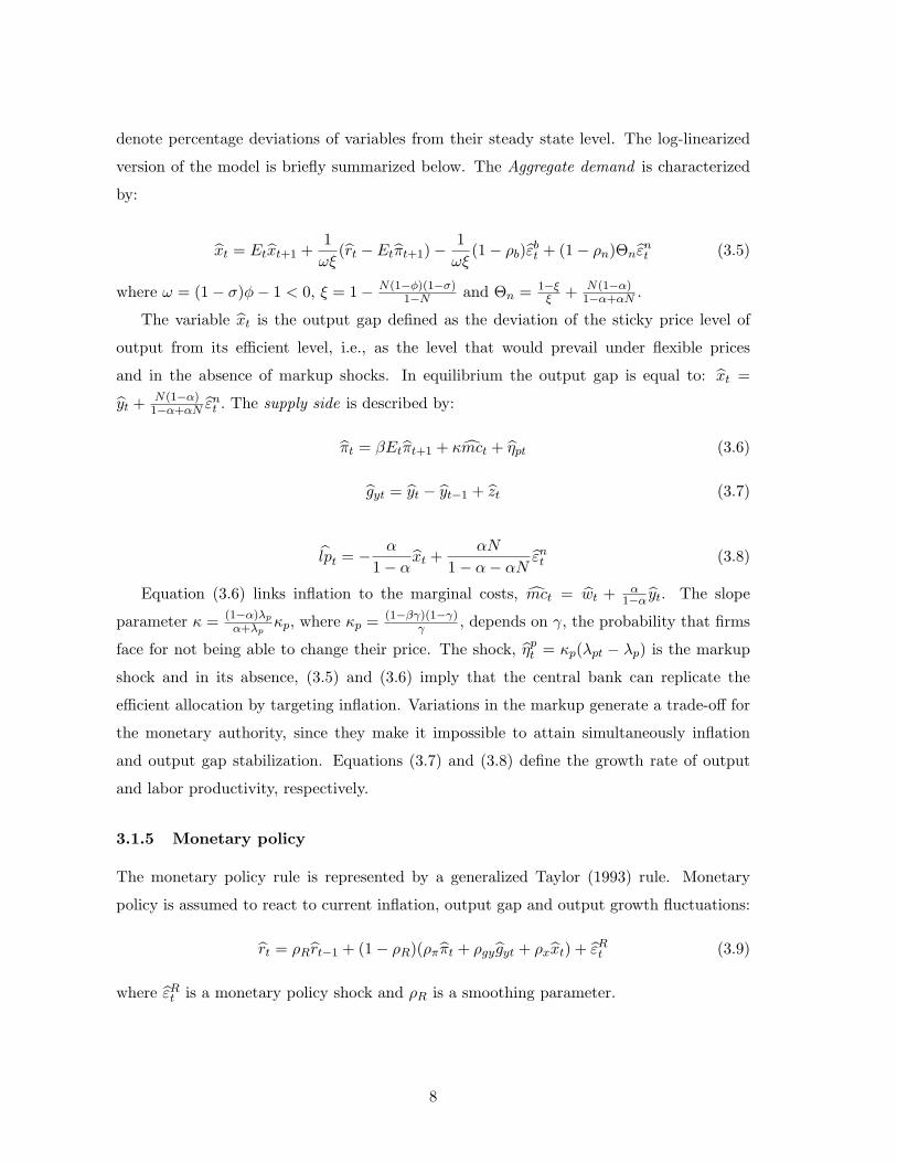
denote percentage deviations of variables from their steady state level. The log-linearized

version of the model is briefly summarized below. The Aggregate demand is characterized

by:

xt = Etxt+1 +1ωξ

(rt − Etπt+1)− 1ωξ

(1− ρb)εbt + (1− ρn)Θnεnt (3.5)

where ω = (1− σ)φ− 1 < 0, ξ = 1− N(1−φ)(1−σ)1−N and Θn = 1−ξ

ξ + N(1−α)1−α+αN .

The variable xt is the output gap defined as the deviation of the sticky price level of

output from its efficient level, i.e., as the level that would prevail under flexible prices

and in the absence of markup shocks. In equilibrium the output gap is equal to: xt =

yt + N(1−α)1−α+αN ε

nt . The supply side is described by:

πt = βEtπt+1 + κmct + ηpt (3.6)

gyt = yt − yt−1 + zt (3.7)

lpt = − α

1− αxt +

αN

1− α− αNεnt (3.8)

Equation (3.6) links inflation to the marginal costs, mct = wt + α1−α yt. The slope

parameter κ = (1−α)λpα+λp

κp, where κp = (1−βγ)(1−γ)γ , depends on γ, the probability that firms

face for not being able to change their price. The shock, ηpt = κp(λpt − λp) is the markup

shock and in its absence, (3.5) and (3.6) imply that the central bank can replicate the

efficient allocation by targeting inflation. Variations in the markup generate a trade-off for

the monetary authority, since they make it impossible to attain simultaneously inflation

and output gap stabilization. Equations (3.7) and (3.8) define the growth rate of output

and labor productivity, respectively.

3.1.5 Monetary policy

The monetary policy rule is represented by a generalized Taylor (1993) rule. Monetary

policy is assumed to react to current inflation, output gap and output growth fluctuations:

rt = ρRrt−1 + (1− ρR)(ρππt + ρgy gyt + ρxxt) + εRt (3.9)

where εRt is a monetary policy shock and ρR is a smoothing parameter.

8

3.1.6 Shocks

The model features five exogenous processes: total factor productivity, zt, labor supply ,

εnt , preference, εbt , monetary policy, εRt , and the price markup shock, λpt. The vector of the

shocks, st = [zt, εnt , εbt , ε

Rt , λpt]

′, is assumed to evolve according to

st = %st−1 + Vt (3.10)

where V is a (5x1) vector of orthogonal White Noise and % is a (5x5) diagonal matrix. We

assume that %1,1 = 1 and |%j,j | < 1 for j 6= 1.

3.2 Theoretical predictions

In this subsection we analyze the theoretical implications of the adoption of inflation tar-

geting in terms of volatilities of output and inflation. In particular we focus on the trade-off

ratio, defined as the ratio between the standard deviations of output growth and inflation

conditional to a mark-up shock, as a measure of the movements along the trade-off curve.

We model the adoption of inflation targeting with a reduction in the coefficients of output

growth, or output gap, ρgy and ρx, from positive values to zero. Alternatively one could

define it as an increase in the parameter ρπ. As it will be clear below results both definitions

yield the same results.

Let us focus first on a simple analytical example. Consider equations (3.5), (3.6) and

(3.9) when all disturbances but the markup shock are set to zero and assume that ρR =

ρgy = 0. Then, the equilibrium conditions under (3.9) are: 1− ρxωξ −ρπ

ωξ

−κx 1

xt

πt

=

1 − 1ωξ

0 β

Etxt+1

Etπt+1

+

0

ηpt

Using the method of undetermined coefficients, we can write the solution as:

xt = a1ηpt

πt = b1ηpt

where

a1 = − ρπ − ρη(ρπ − ρη)κx − ((1− ρη)ωξ − ρx)(1− βρη)

< 0

b1 =ρx − (1− ρη)ωξ

(ρπ − ρη)κx − ((1− ρη)ωξ − ρx)(1− βρη)> 0

9

The trade-off ratio is

TOR =

√V ar(gxt)V ar(πt)

=√

2(ρπ − ρη)

ρx − ωξ(1− ρη)

where ρη is the persistence of the markup shock. Clearly, ∂TOR∂ρπ

> 0 and ∂TOR∂ρx

< 0,

however, we need to show that this prediction holds in the general unrestricted model. To

check whether a reduction to zero of ρgy and ρx yields an increase in the trade-off ratio

we uniformly draw 10000 realizations of the remaining structural parameters parameters

from admissible ranges 5 and check whether the corresponding trade-off ratio increases.

Table 3 indicates that the trade-off ratio increases in 92% and 87% of the parameterizations

respectively. When inflation targeting adoption is defined as an increase in ρπ the trade-off

ratio increases in 96% of the possible parameterizations.

4 Identifying markup shocks

To study the effects of a markup shock we use the methodology of Canova and Paustian

(2008). The exercise consists of two steps:

1. We search for robust implications in terms of the sign of the impact responses of some

variables of interest to a markup shock under various specifications of the theoretical

model of section 3 and check whether such restrictions can uniquely identify the shock.

2. We use these restrictions in a VAR to estimate the shock.

4.1 Robust restrictions

The first step of our procedure is designed to take into consideration the uncertainty in-

volved in calibration exercises. An implication is called robust if it holds independently

of parameterization used. For example, if inflation falls and the output gap increases in

response to markup shocks, regardless of the parameter values, we call this implication

robust. Our method seeks robust implications in terms of sign of the responses which can

be used to identify the shock in the data. Obviously, there may be disturbances which do

not generate robust implications. Also, some shocks may share the same implications. For

example, output increases and inflation falls in response to both TFP and markup shocks.5Admissible ranges for the remaining parameters are: γ ∈ [0.4, 0.9], σ ∈ [1, 4], φ ∈ [0.6, 0.8], α ∈ [0.2, 0.4],

ρη ∈ [0, 0.95].

10

For that reason it is important to establish that none of the other shocks in the model can

generate the same restrictions we use to identify markup shocks.

To implement this first step we uniformly draw all structural parameters from some

specified range (see Appendix B for the details), except β which is set equal to 4%, and

we compute the corresponding impulse response functions. We draw 1000 realizations and

we compute the 84th and 16th percentiles of the simulated distribution for each impulse

response function. If the sign of the two percentiles coincide for some impulse response

function, we call that sign a robust sign restriction.

We summarize the qualitative features of the responses of the variables of interest to

the five shocks in the impact period in Table 4. Figure 1 plots the 68-percent confidence

bands for the responses of these variables to the five shocks. The set of restrictions we use

to identify markup shocks are as follows. Markup shocks should increase output growth,

the real wage and decrease the interest rate and inflation on impact and the response of real

wages to such shocks should be higher than the response of labor productivity. Gambetti and

Pappa (2007) show that these restrictions hold in more general environments with capital

accumulation, rigidities in both the wage and the price setting, and additional frictions,

such as habit in consumption, investment adjustment costs, variable capacity utilization

and wage and price indexation.

In order to ensure that the above restrictions uniquely identify the markup shock, we

examine the responses of the five variables of interest to the other shocks. As it is apparent

from the remaining rows of Table 4, no other shocks can produce the set of restrictions

markup shocks produce. In particular, the sign of the impact effect of the real wage, the

nominal interest rate and inflation to the exogenous disturbances is sufficient to differentiate

the dynamic responses of markup shocks from those of other disturbances in the NK model.

The qualitative restriction on the size of the response of the real wage relative to labor

productivity is crucial for differencing the effects of TFP shocks in an RBC model and

markup shocks in the NK model. Since wages in the NK model are defined as the sum of

labor productivity and marginal costs, real wages tend to increase more in reaction to a

negative markup shock than labor productivity. The conditional responses of the output gap

can also be used to differentiate the two shocks, but since the output gap is unobservable,

the restrictions on the real wage and labor productivity are the only plausible options left

for identification purposes.

11

4.2 Implementing the restrictions in a VAR

For each country we let Yt be a vector including the annual growth rate of real GDP, the

short term nominal interest rate, the annual growth rate of real CPI wage, the annual

growth rate of labor productivity, measured as output per worker, and the annual CPI

inflation rate and assume

A(L)Yt = εt

where A(L) = I − A1L − ... − ApLp, L is the lag operator, p = 2 for all countries and εt

is a Gaussian white noise process with covariance matrix Σ. Let P be the Cholesky factor

of Σ. The markup shock is obtained as emt = h′P−1εt, where h is a unit vector such that

the implied response functions A(L)−1Ph satisfy the identification restrictions of Table 4.

We restrict the responses only in the impact period. To estimate the structural model, we

assume a diffuse prior as in Uhlig (2005) and draw h from a from a uniform distribution

over the unit-sphere. We draw a candidate h and when the restrictions are satisfied we

retain the responses and calculate the statistics of interest. We keep 1000 draws.

5 The evidence

5.1 The identified shocks

Ireland (2004) and Smets and Wouters (2007) (SW henceforth), have estimated implicitly

markup shocks by estimating dynamic stochastic general equilibrium models with nominal

rigidities. They find estimated price markup shocks to be the most important source of

variability in inflation in the short and medium term but to explain a moderate fraction of

output variability. Since in these models markup shocks are modeled as stochastic variations

in the elasticity of substitution between differentiated goods, it is a bit hard to believe that

this type of variations drive inflation dynamics in the US. Furthermore, since in these models

markup shocks play the role of residual shocks, capturing all unmodelled variations in the

data, there are further reasons to doubt the credibility of the estimation outcome. Instead,

our procedure uses part of the information of the model but not all of them and focuses

on qualitative rather than quantitative restrictions. Unsurprisingly, our results differ from

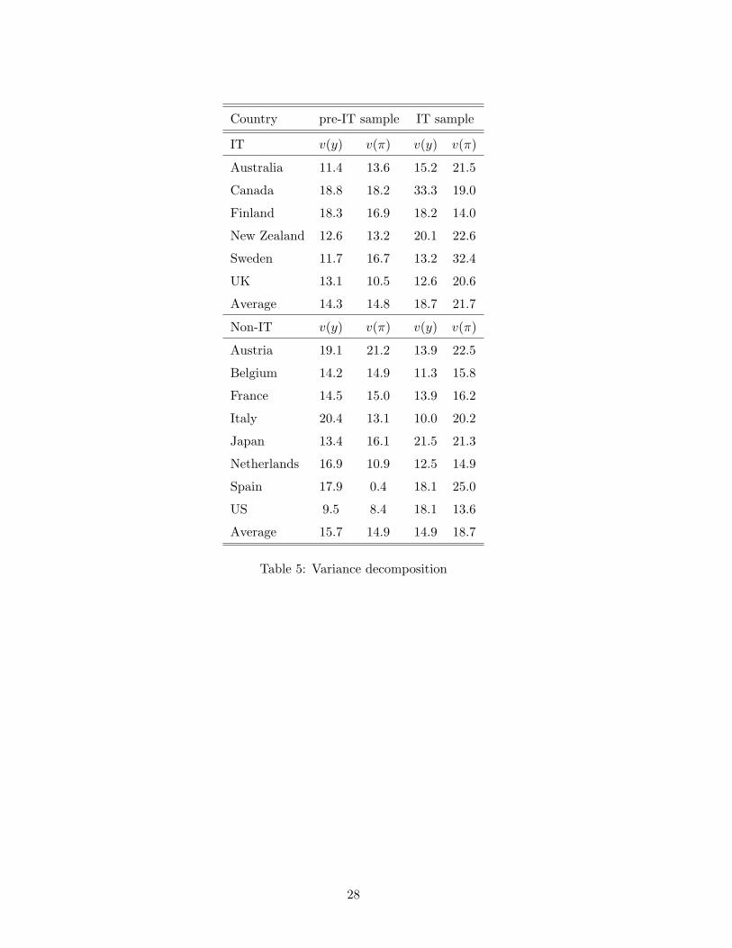
those of SW and Ireland (2004). Table 5 reports the explanatory power of our identified

markup shocks for these two variables at long horizons (45 quarters) for the two groups of

countries.

12

The relative contribution of markup shocks to output growth and inflation variability

in both samples and both groups of countries is moderate and varies between 10% and

20%. Exceptions are Canada for output, and Sweden for inflation in the post 1990 era.

Perhaps more importantly, the importance of markup shocks for inflation and output growth

variability does not seem to have changed across sub periods. Markup shocks matter more

for inflation fluctuations in the IT period for all countries, except Austria and Finland; their

importance for output growth fluctuations increased for Canada, the US and Japan, and

fell significantly for Italy.

Interestingly, since the importance of markup shocks for output and inflation volatility in

the pre-1990 sample is similar in the two groups of countries, the choice of the IT regime does

not appear to be endogenous to the structure of the economy. In other words, policymakers

did not choose an IT regime because markup shocks were less important in their economies.

5.2 Does inflation targeting matter?

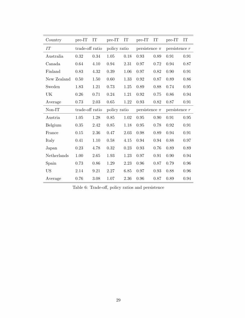
The first two columns of Table 6 report the trade-off ratios for the two sample periods for the

two groups of countries. The emergence of a new policy trade-off is evident in all IT countries

but Sweden and, with the exception of Australia, IT countries have experienced significant

increases in this ratio. However, the increase is also shared by non-IT countries. The

trade-off ratio drastically increases for Japan and France, while for the US and Belgium the

magnitude of the changes is comparable with those of the IT countries. Actually, changes

in the trade-off ratio are higher, on average, for non-IT than for IT countries, although

differences across groups are not statistically significant.

A reason why we fail to detect substantial differences, is that the adoption of the IT

regime could have coincided with other changes that more significantly altered the structure

of the economies.6 Cecchetti and Ehrmann (2000) suggest that the environment of the

1990s was generally benevolent and that the choice of monetary policy strategy, within a

class of reasonable strategies, might have been irrelevant. However, when we examine the

performance of IT countries versus non IT countries in the post 1990 period, we also fail

to detect differences between the two groups. Inflation targeting countries have an average

trade-off ratio of about 2, while non IT countries have an average ratio of about 3, although6Part of these results might be due to the Great Moderation (see, McConnell and Perez Quiroz, (2000),

Cogley and Sargent (2001, 2005), Sims and Zha (2006), Stock y Watson (2003), and Gambetti, et.al. (2005),

among others), since the pre-IT sample includes periods of high inflation and output volatility relative to

the post IT period where both inflation and output volatility had been more moderate for all countries.

13

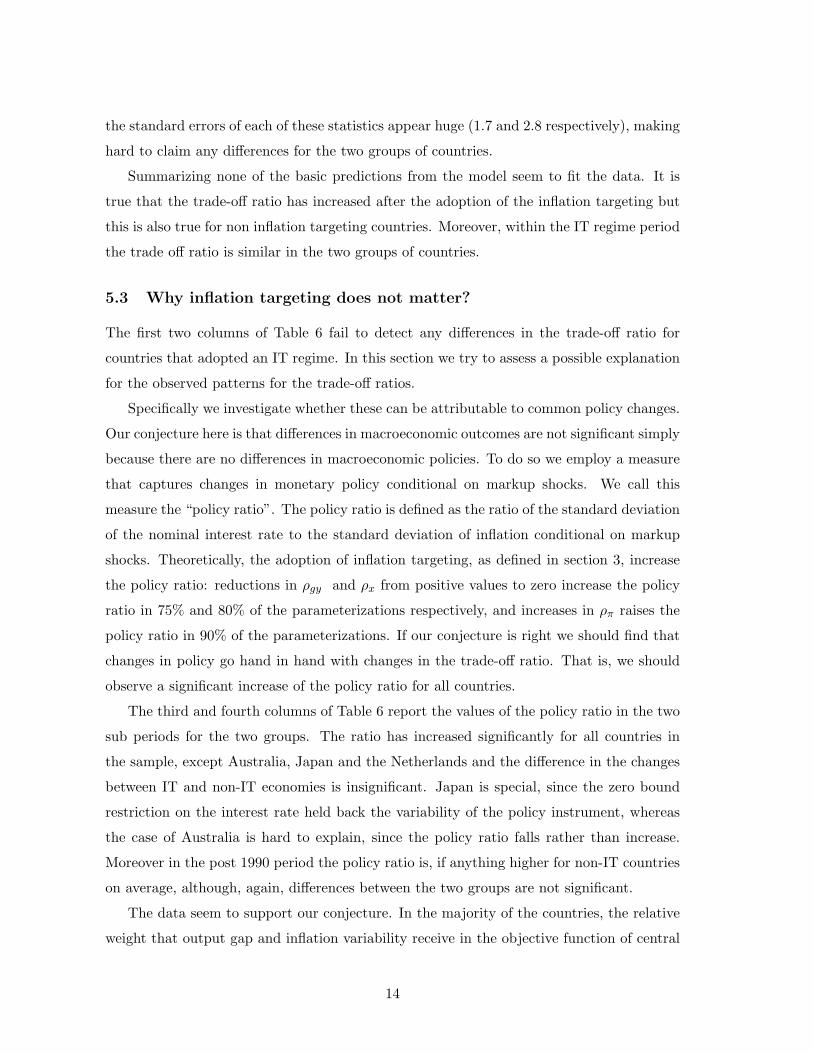
the standard errors of each of these statistics appear huge (1.7 and 2.8 respectively), making

hard to claim any differences for the two groups of countries.

Summarizing none of the basic predictions from the model seem to fit the data. It is

true that the trade-off ratio has increased after the adoption of the inflation targeting but

this is also true for non inflation targeting countries. Moreover, within the IT regime period

the trade off ratio is similar in the two groups of countries.

5.3 Why inflation targeting does not matter?

The first two columns of Table 6 fail to detect any differences in the trade-off ratio for

countries that adopted an IT regime. In this section we try to assess a possible explanation

for the observed patterns for the trade-off ratios.

Specifically we investigate whether these can be attributable to common policy changes.

Our conjecture here is that differences in macroeconomic outcomes are not significant simply

because there are no differences in macroeconomic policies. To do so we employ a measure

that captures changes in monetary policy conditional on markup shocks. We call this

measure the “policy ratio”. The policy ratio is defined as the ratio of the standard deviation

of the nominal interest rate to the standard deviation of inflation conditional on markup

shocks. Theoretically, the adoption of inflation targeting, as defined in section 3, increase

the policy ratio: reductions in ρgy and ρx from positive values to zero increase the policy

ratio in 75% and 80% of the parameterizations respectively, and increases in ρπ raises the

policy ratio in 90% of the parameterizations. If our conjecture is right we should find that

changes in policy go hand in hand with changes in the trade-off ratio. That is, we should

observe a significant increase of the policy ratio for all countries.

The third and fourth columns of Table 6 report the values of the policy ratio in the two

sub periods for the two groups. The ratio has increased significantly for all countries in

the sample, except Australia, Japan and the Netherlands and the difference in the changes

between IT and non-IT economies is insignificant. Japan is special, since the zero bound

restriction on the interest rate held back the variability of the policy instrument, whereas

the case of Australia is hard to explain, since the policy ratio falls rather than increase.

Moreover in the post 1990 period the policy ratio is, if anything higher for non-IT countries

on average, although, again, differences between the two groups are not significant.

The data seem to support our conjecture. In the majority of the countries, the relative

weight that output gap and inflation variability receive in the objective function of central

14

banks must have changed. This conclusion, however, is hard to reconcile with the fact that

some countries have announced an IT regime and other countries have not, unless actions

speak by themselves and announcing an inflation target does not matter.

Can other structural changes account for these patterns? In theory, increases in the

coefficient of relative risk aversion, σ, increase the policy ratio but make the trade-off and

the policy ratio move in opposite directions. This is because increases in the relative risk

aversion coefficient reduce the responsiveness of output to changes in the interest rate,

therefore decreasing output variability and the trade-off ratio. At the same time, since they

limit the effects of markup shocks on demand and, hence, on inflation, the policy ratio

must increase. Thus, changes in the preferences of the agents in non-IT countries, could be

responsible for the similarities between non-IT and IT countries if increases in the trade-off

ratio are accompanied by decreases in the policy ratio. As table 4 suggest, this is the case

only for the Netherlands.

Reductions in the degree of price stickiness, γ, or the persistence of the markup shock,

ρη, can increase the two ratios with a relatively high probability (in 52% of the param-

eterizations of the model). They also induce reductions in the conditional persistence of

inflation and the interest rate: in the model a fall in γ decreases inflation and interest rate

persistence in 70% of the parameterizations of the model and a fall in the persistence of the

shock always reduces persistence in both series (in 97% of the parameterizations for inflation

and in 99% of the parameterizations for the interest rate). Could differential changes in

these two parameters across the two groups of countries be responsible for the fact that the

performance of IT and non-IT countries is similar? The last four columns of Table 6 report

the conditional AR(1) coefficients of CPI inflation and interest rate in the two groups of

countries for the two sub periods. Inflation persistence dropped in all countries in the second

subsample. Targeting countries experienced a larger decrease in inflation persistence rela-

tive to non-targeting ones, but difference-in-differences estimates (see Appendix C, Panel I)

are imprecise and indicate that differences are insignificant. Changes in the conditional per-

sistence of nominal interest rates are more heterogeneous - persistence has remained almost

unchanged in Australia, and Finland (which are targeters) and Belgium and Japan (which

are non-targeters) it has increased in seven countries (UK and Sweden from IT and US,

Spain, the Netherlands, Austria and Italy from non-IT) and it has fallen for the remaining

three countries - but, overall inconsistent with the idea that non-IT economies experienced

a relatively larger reduction in the shock persistence or in the degree of nominal rigidities.

15

Differences across countries in the post 1990 period are also insignificant, so we are led to

conclude that the only structural change compatible with the evidence is an increase in the

aversion of policymakers to inflation fluctuations in the last decades.

6 Robustness

6.1 Supply shocks

In our analysis so far we have implicitly assumed that policymakers face a trade-off between

output gap and inflation fluctuations. However, output growth might matter more than

output gap measures for policy decisions in practice. In this case, in fact, TFP and labor

supply shocks may also induce a trade-off between output and inflation stabilization (see

Table 4). Therefore, by examining how the ratios behave in response to these shocks, one

can draw firmer conclusions on the importance of the IT regime for output and inflation

fluctuations.

Rather than separately identifying TPF and labor supply shocks, which is hard to do in

the context of the model, since the implications they produce are not necessarily robust, we

identify a generic supply shock, imposing the restriction that it moves output growth and

inflation in opposite directions on impact, and examine whether the conclusions we have

reached change, conditional on this generic shock.

Table 7, which contains the estimated trade-off and policy ratios, has the same quali-

tative message as Table 6: both the trade-off and the policy ratios conditional on supply

shocks have increased across sub periods, and the increase is similar for both IT and non-IT

economies. Also averages of the two ratios are not significantly different in the post 1990

period. Both the trade-off and the policy ratio are higher for non IT countries in the last

subsample, but given standard errors, differences are insignificant. Given that these generic

supply shocks explain a higher percentage of output and inflation fluctuations (on average

40% of output and 30% of inflation fluctuations), failure to find any difference between IT

and non-IT countries is even more striking in this case.

6.2 Changes in expectations

Changes in inflation expectations after the adoption of an IT regime could have affected the

dynamics of output and inflation in response to markup shocks. With a more credible regime

policymakers could have reduced inflation without having to sacrifice output variability

16

by affecting inflation expectations, producing an inward shift in the trade-off curve that

our measures cannot capture. To examine such a possibility we repeated our exercise

adding long term rates to our VAR. Studying a system with the long term rate shields us

from the possibility that the results we have obtained are spurious and due to omission of

inflation expectation proxies. We present results in Table 87. Results in Table 8 are directly

comparable qualitatively with the results in Table 6. The magnitude of the changes in the

trade-off and policy ratios in the two groups of countries is unaffected by the addition of

long term rates. Except for Spain, the behavior of the trade-off ratio in the pre-IT relative

to the IT period mimics the one of the specification without inflation expectations. The

same is true for the policy ratio, except for the movements in the policy ratio in Austria.

Again, for the IT period differences in the mean of the ratios between IT and non IT

countries are insignificant. Hence, even controlling for changes in inflation expectations,

the macroeconomic performance of the two groups of countries is similar.

7 Conclusions

The paper examines whether the adoption of an IT regime affects macroeconomic per-

formance, when we condition the analysis on a shock that generates a trade-off between

inflation and output stabilization purposes. The theory provides clear cut predictions that

can be tested in the data. In fact, in any DSGE model with nominal rigidities, a change

in the relative weight that output and inflation variability have in the objective function

of central banks implies movements along the output-inflation variability trade-off curve

toward a region where inflation is less and output is more variable than it would otherwise

have been. A movement of this type is present in the data but its size does not differ for

IT and non-IT countries.

Our measure of the policy stance, the policy ratio, reveals similar changes in the behavior

of non-IT and IT countries. We also show that the similarities in performance are not due

to the peculiarity of the identified markup shocks - generic supply shocks generate similar

pictures and that changes in inflation expectations induced by a generalized improvement

of credibility cannot account for the empirical pattern either. Our analysis leads us to

conclude that announcing an IT regime does not matter for output and inflation dynamics

as long as monetary policy put sufficient importance to inflation stabilization.

7Finland is not included in this analysis due to shortage of series for long term rates.

17

Appendix A

The appendix presents provides a brief description of the data used for each of the countries

considered in the sample.

Variable Source Definition

RGDP OECD Real Gross Domestic Product

HOURS OECD/IFS Total Hours Worked per employee in the Business Sector

TOTEMP OECD/IFS Total employment

WAGES OECD/IFS Wages and Salaries of employees (net wage + social security contributions)

COMP OECD net wage + social security contributions paid by employees and employers

INT IFS short term nominal (money market) rate

CPI IFS/OECD consumer price index

LONG INT IFS/OECD yield 10-year government bond

Table A1: Data: sources and definitions

18

Appendix B

Parameter Description Range

β discount factor 1.04−1/4

σ risk aversion coefficient [1,4]

φ determines steady state level of hours [0.6,0.8]

1− α labor share [0.6,0.8]

z steady state growth rate [1.004,1.0055]

λp steady state markup [0.0,0.25]

γ degree of price stickiness [0.4,0.9]

ρR lagged interest rate coefficient [0.2,0.9]

ρπ inflation coefficient on interest rate rule [1.1,5.0]

ρx output gap coefficient on interest rate rule [0.0,1.0]

ρgy output growth coefficient on interest rate rule [0.0,1.0]

% persistence of shocks [0,0.97]

Table B1: Parameter ranges

19

Appendix C

Difference-in-differences regressions

Xpost −Xpre = a0 + a1D + a2Xpre + e

Xpost : a country’s statistic X in the IT period

Xpre : a country’s statistic X in the pre-IT period

D : dummy variable which is one if a country adopted IT

X measures/ coefficients a0 a1 a2 Adj. R2

PANEL I: Conditional on markup shocks, basic VAR

trade-off ratio 1.62 (1.08) -0.99 (1.17) 0.92 (1.00) -0.03

Policy ratio 0.79 (0.99) -0.53 (0.89) 0.46 (0.77) -0.07

Persistence π 1.41 (0.86) -0.06 (0.04) -1.57 (0.90) 0.10

Persistence r 1.26 (0.12) -0.04 (0.015) -1.36 (0.13) 0.88

PANEL II: Conditional on markup shocks, VAR with long term rates

trade-off ratio 1.68 (0.83) -1.06 (0.96) 0.43 (0.70) -0.03

Policy ratio 0.57 (1.08) -0.45 (0.95) 0.61 (0.85) 0.10

PANEL III: Conditional on supply shocks, basic VAR

trade-off ratio 2.87 (1.03) -1.05 (1.13) 0.06 (0.46) -0.08

Policy ratio 0.96 (1.81) -1.02 (1.46) 1.65 (1.37) 0.05

Table C1: Difference in difference regressions (standard errors are in parenthesis).

20

References

[1] Ball, L., Sheridan, N., (2003), Does Inflation Targeting Make a Difference? in Woodford

M., and Bernanke, B. eds., Inflation Targeting, Boston, NBER.

[2] Ball, L., Mankiw, N., G., and R. Reis. (2005), “Monetary Policy for Inattentive

Economies.” Journal of Monetary Economics, 52, 703–25.

[3] Benati, L., (2008), ”Investigating Inflation Persistence Across Monetary Regimes,”

ECB Working Paper Series, No. 851.

[4] Bernanke, B. S., Laubach, T., Mishkin,F.S. and A. S. Posen. (1999), ”Inflation Target-

ing: Lessons from the International Experience,” Princeton University Press: Prince-

ton, N.J.

[5] Boivin, J. and M. Giannoni (2002), ”Has Monetary Policy Become Less Powerful?”,

Columbia Business School, mimeo.

[6] Calvo, G. (1983), ”Staggered pricing in a utility maximizing framework,” Journal of

Monetary Economics, Vol. 12, pp. 383-96.

[7] Canova, F., Gambetti, L. and E. Pappa (2007), ”The structural dynamics of output

growth and inflation: some international evidence” Economic Journal, Vol. 117, 519,

pp. C167-C191.

[8] Canova F., Cicarelli, M. and E. Ortega (2006), ”Do political events affect business

cycles? The Maastricht treaty, the creation of the ECB and the Euro economy,” mimeo

UPF.

[9] Canova F. and M. Paustian (2008), ”Measurment with some theory: Using sign re-

strictions to eveluate business cycle models,” mimeo UPF.

[10] Cecchetti, S. and M. Ehrmann (2001), “Does Inflation Targeting Increase Output

Volatility? An International Comparison of Policymakers’ Preferences and Outcomes,”

in N. Loayza and K. Schmidt-Hebbel (ed.) Monetary Policy: Rules and Transmission

Mechanisms, Central Bank of Chile.

[11] Clarida, R., J. Gali and M. Gertler (2000), ”Monetary Policy Rule and Macroeconomic

Stability: Evidence and Some Theory”, Quarterly Journal of Economics, CXV, pp.

147-180.

21

[12] Cogley, T. and T.J. Sargent (2001), ”Evolving Post-World War II U.S. Inflation Dy-

namics”, NBER Macroeconomic Annual, 16,

[13] Cogley, T. and T.J. Sargent (2005), ”Drifts and Volatilities: Monetary Policies and

Outcomes in the Post WWII U.S.”, Review of Economic Dynamics, Vol. 8, 2, pp.

262-302.

[14] Cohen, V., Gonzalez, M. and A. Powell (2003), “A New Test for the Success of Inflation

Targeting,” Universidad Torcuato Di Tella mimeo., January 2003.

[15] Corbo, V., Landerretche, O. and K. Schmidt-Hebbel (2002), “Does Inflation Targeting

Make a Difference?” in Norman Loayza and Raimundo Soto, eds., Inflation Targeting:

Design, Performance, Challenges (Central Bank of Chile: Santiago): 221-269.

[16] Erceg, C., Henderson, D. and A. Levin (2000), “Optimal Monetary Policy with Stag-

gered Wage and Price Contracts.” Journal of Monetary Economics, 46, 281–313.

[17] Ireland, P. (2004), ”Technology shocks in New Keynesian models,” The Review of

Economics and Statistics, 924-936.

[18] Gambetti, L., Pappa, E. and F. Canova (2005), ”The structural dynamics of US output

and inflation: what explains the changes?” forthcoming Journal of Money Credit and

Banking.

[19] Gambetti, L. and E. Pappa. (2007), ”Markup shocks: Is there a trade-off between

output and inflation stabilization?” mimeo UAB.

[20] Levin, A., Natalucci, F. and J. M. Piger (2004). “The Macroeconomic Effects of Infla-

tion Targeting,” Federal Reserve Bank of St. Louis Review, 86, 51-80.

[21] McConnell, M. and Perez Quiroz, G. (2001), ”Output fluctuations in the US: what has

changed since the early 1980s? ”, American Economic Review, 90, 1464-1476.

[22] Mishkin, F. and K. Schmidt-Hebbel (2007), ”Does Inlfation Targeting Make a Differ-

ence?” NBER Working Paper Series, No. w12876.

[23] Mishkin, F. (2004), ”Why the Federal Reserve Should Adopt Inflation Targeting,”

International Finance, 7, 1, pp.117-127.

[24] Sims, C.A. and T. Zha (2006), ”Were there Regime Switches in US Monetary Policy”,

American Economic Review, 96, 1, pp. 54-81.

22

[25] Smets, F. and R. Wouters (2003), “An Estimated Dynamic Stochastic General Equi-

librium Model of the Euro Area.” Journal of the European Economic Association, 1,

1123–1175.

[26] Smets, F. and R. Wouters (2007), “Shocks and Frictions in U.S. Business Cycles: A

Bayesian DSGE Approach.” Working paper, European Central Bank, No 722.

[27] Steinsson, J. (2003), “Optimal Monetary Policy in an Economy with Inflation Persis-

tence.” Journal of Monetary Economics, 50, 1425–56.

[28] Stock, J. and M. Watson (2003), “Has the business cycle changed? Evidence and

explanations”, in: Monetary policy and uncertainty, Federal Reserve Bank of Kansas

City, 9-56.

[29] Taylor, J (1993), ”Discretion versus policy rules in practice,” Carnegie-Rochester Con-

ference Series on Public Policy, Vol. 39, pp. 195-214.

[30] Uhlig, H. (2005), ”What are the effects of monetary policy on output? Results from

an agnostic identification procedure,” Journal of Monetary Economics 52, 381–419.

23

Tables

Country pre-IT sample IT sample

IT:

Australia 1970:1-1994:3 1994:4-2007:1

Canada 1970:1-1993:4 1994:1-2007:1

Finland 1970:1-1993:4 1994:1-1998:4

New Zealand 1970:1-1992:4 1993:1-2007:1

Sweden 1970:1-1994:4 1995:1-2007:1

UK 1970:1-1992:4 1993:1-2007:1

Non IT:

Austria 1970:1-1993:4 1994:1-2007:1

Belgium 1980:1-1993:4 1994:1-2007:1

France 1970:1-1993:4 1994:1-2007:1

Italy 1971:1-1993:4 1994:1-2007:1

Japan 1970:1-1993:4 1994:1-2007:1

Netherlands 1970:1-1993:4 1994:1-2007:1

Spain 1977:1-1993:4 1994:1-2007:1

US 1970:1-1993:4 1994:1-2007:1

Table 1: Regime periods.

24

Country v(y)preIT v(y)IT v(π)preIT v(π)IT v(y)preIT

v(π)preITv(y)IT

v(π)IT

IT

Australia 2.34 1.08 3.67 1.50 0.64 0.71

Canada 2.53 1.39 2.95 0.88 0.86 1.57

Finland 3.49 1.53 3.92 0.85 0.89 1.80

New Zealand 5.25 1.78 4.59 1.10 1.14 1.63

Sweden 3.64 1.82 2.78 1.02 1.31 1.79

UK 2.55 0.77 5.19 0.67 0.49 1.14

Average 3.30 1.40 3.85 1.00 0.89 1.44

Non IT

Austria 2.18 1.14 2.12 0.79 1.03 1.44

Belgium 1.47 0.74 2.21 0.51 0.66 1.47

France 1.63 1.07 3.58 0.60 0.45 1.80

Italy 2.56 1.30 5.08 1.05 0.50 1.23

Japan 2.30 1.64 4.76 0.81 0.48 2.03

Netherlands 2.27 1.40 2.99 0.79 0.76 1.77

Spain 2.06 1.01 4.27 0.92 0.48 1.10

US 3.45 1.52 2.34 0.56 1.47 2.69

Average 3.30 1.40 3.85 1.00 0.73 1.69

Table 2: Unconditional statistics

25

Parameters Ranges Prob(↑ TOR)

ρgy [0.2,1],0 87%

ρx [0.2,1],0 92%

ρπ [1,5] 96%

Table 3: Parameter changes and probabilities of an increase in TOR.

26

gyt πt rt wt wt − lpt yt xt

Markup + − − + + + +

TFP + − − + −

Labor Supply + − − − + −

Preference + + + + + + +

Monetary Policy + + − + + + +

Table 4: Sign restrictions.

27

Country pre-IT sample IT sample

IT v(y) v(π) v(y) v(π)

Australia 11.4 13.6 15.2 21.5

Canada 18.8 18.2 33.3 19.0

Finland 18.3 16.9 18.2 14.0

New Zealand 12.6 13.2 20.1 22.6

Sweden 11.7 16.7 13.2 32.4

UK 13.1 10.5 12.6 20.6

Average 14.3 14.8 18.7 21.7

Non-IT v(y) v(π) v(y) v(π)

Austria 19.1 21.2 13.9 22.5

Belgium 14.2 14.9 11.3 15.8

France 14.5 15.0 13.9 16.2

Italy 20.4 13.1 10.0 20.2

Japan 13.4 16.1 21.5 21.3

Netherlands 16.9 10.9 12.5 14.9

Spain 17.9 0.4 18.1 25.0

US 9.5 8.4 18.1 13.6

Average 15.7 14.9 14.9 18.7

Table 5: Variance decomposition

28

Country pre-IT IT pre-IT IT pre-IT IT pre-IT IT

IT trade-off ratio policy ratio persistence π persistence r

Australia 0.32 0.34 1.05 0.18 0.93 0.89 0.91 0.91

Canada 0.64 4.10 0.94 2.31 0.97 0.72 0.94 0.87

Finland 0.83 4.32 0.39 1.06 0.97 0.82 0.90 0.91

New Zealand 0.50 1.50 0.60 1.33 0.92 0.87 0.89 0.86

Sweden 1.83 1.21 0.73 1.25 0.89 0.88 0.74 0.95

UK 0.26 0.71 0.24 1.21 0.92 0.75 0.86 0.94

Average 0.73 2.03 0.65 1.22 0.93 0.82 0.87 0.91

Non-IT trade-off ratio policy ratio persistence π persistence r

Austria 1.05 1.28 0.85 1.02 0.95 0.90 0.91 0.95

Belgium 0.35 2.42 0.85 1.18 0.95 0.78 0.92 0.91

France 0.15 2.36 0.47 2.03 0.98 0.89 0.94 0.91

Italy 0.41 1.10 0.58 4.15 0.94 0.94 0.88 0.97

Japan 0.23 4.78 0.32 0.23 0.93 0.76 0.89 0.89

Netherlands 1.00 2.65 1.93 1.23 0.97 0.91 0.90 0.94

Spain 0.73 0.86 1.29 2.23 0.96 0.87 0.79 0.96

US 2.14 9.21 2.27 6.85 0.97 0.93 0.88 0.96

Average 0.76 3.08 1.07 2.36 0.96 0.87 0.89 0.94

Table 6: Trade-off, policy ratios and persistence

29

Country pre-IT IT pre-IT IT

IT trade-off ratio policy ratio

Australia 0.46 0.58 1.28 0.28

Canada 0.94 3.85 1.11 4.36

Finland 1.11 6.55 0.44 2.49

New Zealand 1.03 2.58 0.83 1.80

Sweden 2.31 2.81 0.91 1.77

UK 0.34 1.06 0.26 1.74

Average 1.03 2.9 0.8 2.07

Non-IT trade-off ratio policy ratio

Austria 1.38 2.67 1.23 1.57

Belgium 0.42 4.18 0.83 1.80

France 0.28 2.79 0.58 4.31

Italy 4.35 7.35 1.35 8.37

Japan 0.29 6.58 0.33 0.35

Netherlands 1.89 3.66 1.69 1.25

Spain 0.68 1.06 0.81 4.00

US 3.37 8.04 2.25 10.2

Average 1.58 4.54 1.14 3.98

Table 7: trade-off and policy ratios / supply shock

30

Country pre-IT IT pre-IT IT

IT trade-off ratio policy ratio

Australia 0.41 0.40 1.13 0.17

Canada 0.73 3.65 0.97 2.36

New Zealand 0.61 2.31 0.64 1.41

Sweden 1.82 1.47 0.79 0.87

UK 0.21 0.75 0.20 1.66

Average 0.76 1.51 0.54 1.32

non-IT trade-off ratio policy ratio

Austria 1.06 1.42 0.99 0.94

Belgium 0.33 2.11 0.91 1.25

France 0.23 2.30 0.60 1.86

Italy 0.40 1.61 0.59 4.37

Japan 0.23 4.37 0.35 0.23

Netherlands 0.87 2.79 1.60 1.33

Spain 1.06 0.95 1.26 1.83

US 3.37 7.58 2.38 6.69

Average 0.84 2.89 1.08 2.31

Table 8: trade-off and policy ratios / inflation expectations

31

Figures

Figure 1: 68-percent confidence bands for the responses of the variables in response to

markup (first column), a productivity (second column), a labor supply (third column), a

preference (forth column) and a monetary policy shock (last column).

32