dos and don’ts of reduced chi-squared - arxiv.org e ... · pdf filedos and don’ts...

Dos and don’ts of reduced chi-squared

Rene Andrae1, Tim Schulze-Hartung1 & Peter Melchior2

1 Max-Planck-Institut fur Astronomie, Konigstuhl 17, 69117 Heidelberg, Germany

2 Institut fur Theoretische Astrophysik, ZAH, Albert-Ueberle-Str. 2, 69120 Heidelberg, Germany

e-mail: [email protected]

Reduced chi-squared is a very popular method for model assessment, model comparison,convergence diagnostic, and error estimation in astronomy. In this manuscript, we discussthe pitfalls involved in using reduced chi-squared. There are two independent problems:(a) The number of degrees of freedom can only be estimated for linear models. Concerningnonlinear models, the number of degrees of freedom is unknown, i.e., it is not possible tocompute the value of reduced chi-squared. (b) Due to random noise in the data, alsothe value of reduced chi-squared itself is subject to noise, i.e., the value is uncertain.This uncertainty impairs the usefulness of reduced chi-squared for differentiating betweenmodels or assessing convergence of a minimisation procedure. The impact of noise on thevalue of reduced chi-squared is surprisingly large, in particular for small data sets, whichare very common in astrophysical problems. We conclude that reduced chi-squared canonly be used with due caution for linear models, whereas it must not be used for nonlinearmodels at all. Finally, we recommend more sophisticated and reliable methods, which arealso applicable to nonlinear models.

1 Introduction

When fitting a model f with parameters ~θ to N data values yn, measured with (uncorrelated)Gaussian errors σn at positions ~xn, one needs to minimise

χ2 =N∑n=1

(yn − f(~xn; ~θ)

σn

)2

. (1)

This is equivalent to maximising the so-called “likelihood function”. If the data’s measurementerrors are not Gaussian, χ2 should not be used because it is not the maximum-likelihoodestimator. For the rest of this manuscript, we shall therefore assume that the data’s errors areGaussian. If K denotes the number of degrees of freedom, reduced χ2 is then defined by

χ2red =

χ2

K. (2)

χ2red is a quantity widely used in astronomy. It is essentially used for the following purposes:

1. Single-model assessment: If a model is fitted to data and the resulting χ2red is larger than

one, it is considered a “bad” fit, whereas if χ2red < 1, it is considered an overfit.

2. Model comparison: Given data and a set of different models, we ask the question whichmodel fits the data best. Typically, each model is fit to the data and their values of χ2

red

are compared. The winning model is that one whose value of χ2red is closest to one.

1

arX

iv:1

012.

3754

v1 [

astr

o-ph

.IM

] 1

6 D

ec 2

010

Andrae et al. (2010) – Dos and don’ts of reduced χ2

3. Convergence diagnostic: A fit is typically an iterative process which has to be stoppedwhen converged. Convergence is sometimes diagnosed by monitoring how the value ofχ2

red evolves during the iteration and the fit is stopped as soon as χ2red reaches a value

sufficiently close to one. Sometimes it is claimed then, that “the fit has reached noiselevel”.

4. Error estimation: One fits a certain model to given data by minimising χ2 and thenrescales the data’s errors such that the value of χ2

red is exactly equal to one. From thisone then computes the errors of the model parameters. (It has already been discussed byAndrae (2010) that this method is incorrect, so we will not consider it any further here.)

In all these cases, χ2red excels in simplicity, since all one needs to do is divide the value of χ2 by

the number of degrees of freedom and compare the resulting value of χ2red to one.

In this manuscript, we want to investigate the conditions under which the aforementionedapplications are meaningful – at least the first three. In particular, we discuss the pitfalls thatmay severly limit the credibility of these applications. We explain the two major problems thattypically arise in using χ2

red in practice: First, we dicuss the issue of estimating the number ofdegrees of freedom in Sect. 2. Second, we explain how the uncertainty in the value of χ2 mayaffect the above applications in Sect. 3. Section 4 is then dedicated to explain more reliablemethods rather than χ2

red. We conclude in Sect. 5.

2 Degrees of freedom

Given the definition of χ2red, it is evidently necessary to know the number of degrees of freedom

of the model. For N data points and P fit parameters, a naıve guess is that the number ofdegrees of freedom is N − P . However, in this section, we explain why this is not true ingeneral. We begin with a definition of “degrees of freedom” and then split this discussion intothree parts: First, we discuss only linear models. Second, we discuss linear models with priors.Third, we discuss nonlinear models. Finally, we discuss whether linearisation may help in thecase of nonlinear models.

2.1 Definition

For a given parameter estimate, e.g., a model fitted to data, the degrees of freedom are thenumber of independent pieces of information that were used. The concept of “degrees offreedom” can be defined in different ways. Here, we give a general and simple definition. Inthe next section, we give a more technical definition that only applies to linear models.

Let us suppose that we are given N measurements yn and a model with P free parametersθ1, θ2, . . . , θP . The best-fitting parameter values are found by minimising χ2. This means weimpose P constraints of the type

∂χ2

∂θp= 0 ∀p = 1, 2, . . . , P (3)

onto our N -dimensional system. Hence, the number of degrees of freedom is K = N − P . Atfirst glance, this appears to be a concise and infallible definition. However, we shall see thatthis is not the case.

2


2.2 Linear models without priors

A linear model is a model, where all fit parameters are linear. This means it is a linearsuperposition of a set of basis functions,

f(~x, ~θ) = θ1B1(~x) + θ2B2(~x) + . . .+ θPBP (~x) =P∑p=1

θpBp(~x) , (4)

where the coefficients θp are the fit parameters and the Bp(~x) are some (potentially nonlinear)functions of the position ~x. A typical example is a polynomial fit, where Bp(x) = xp. Insertingsuch a linear model into χ2 causes χ2 to be a quadratic function of the fit parameters, i.e.,the first derivatives – our constraints from Eq. (3) – form a set of linear equations that can besolved analytically under certain assumptions.

A natural approach to solve such sets of linear equations is to employ linear algebra. Thiswill lead us to a quantitative definition of the number of degrees of freedom for linear models.Let us introduce the following quantities:

• ~y = (y1, y2, . . . , yN)T is the N -dimensional vector of measurements yn.

• ~θ = (θ1, θ2, . . . , θP )T is the P -dimensional vector of linear model parameters θp.

• Σ is the N ×N covariance matrix of the measurements, which is diagonal in the case ofEq. (1), i.e., Σ = diag(σ2

1, σ22, . . . , σ

2N).

• X is the so-called design matrix which has format N × P . Its elements are given byXnp = Bp(~xn), i.e., the p-th basis function evaluated at the n-th measurement point.

Given these definitions, we can now rewrite Eq. (1) in matrix notation,

χ2 = (~y −X · ~θ)T ·Σ−1 · (~y −X · ~θ) . (5)

Minimising χ2 by solving the constraints of Eq. (3) then yields the analytic solution

~θ = (XT ·Σ−1 ·X)−1 ·XT ·Σ−1 · ~y , (6)

where the hat in ~θ accounts for the fact that this is only an estimator for ~θ, but not the true ~θitself. We then obtain the prediction ~y of the measurements ~y by,

~y = X · ~θ = X · (XT ·Σ−1 ·X)−1 ·XT ·Σ−1 · ~y = H · ~y , (7)

where we have introduced the N × N matrix H , which is sometimes called “hat matrix”,because it translates the data ~y into a model prediction ~y. The number of effective modelparameters is then given by the trace of H (e.g. Ye 1998; Hastie et al. 2009),

Peff = tr(H) =N∑n=1

Hnn = rank(X) , (8)

which also equals the rank of the design matrix X.1 Obviously, Peff ≤ P , where the equalityholds if and only if the design matrix X has full rank. Consequently, for linear models thenumber of degrees of freedom is

K = N − Peff ≥ N − P . (9)

1The rank of X equals the number of linearly independent column vectors of X.

3


The standard claim is that a linear model with P parameters removes P degrees of freedomwhen fitted to N data points, such that the remaining number of degrees of freedom is K = N−P . Is this correct? No, not necessarily so. The problem is in the required linear independenceof the P basis functions. We can also say that the P constraints given by Eq. (3) are notautomatically independent of each other. Let us consider a trivial example, where the basisfunctions are clearly not linearly independent:

Example 1 The linear model f(~x, ~θ) = θ1 + θ2 is composed of two constants, θ1 and θ2, i.e.,B1(~x) = B2(~x) = 1. Obviously, this two-parameter linear model cannot fit two arbitrary datapoints and its number of degrees of freedom is not given by N − 2 but N − 1, because the designmatrix X only has rank 1, not rank 2. In simple words, the two constraints ∂χ2

∂θ1= 0 and ∂χ2

∂θ2= 0

are not independent of each other.

From this discussion we have to draw the conclusion that for a linear model the number ofdegrees of freedom is given by N −P if and only if the basis functions are linearly independentfor the given data positions ~xn, which means that the design matrix X has full rank. In practice,this condition is usually satisfied, but not always. In the more general case, the true numberof degrees of freedom for a linear model may be anywhere between N − P and N − 1.

2.3 Linear models with priors

Figure 1: Example of a two-parametermodel, f(x) = a0 + a1x, that is incapableof fitting two data points perfectly becauseit involves a prior a1 ≥ 0. We show the op-timal fit for the given data. The model isdiscussed in Example 2.

Priors are commonly used to restrict the possiblevalues of fit parameters. In practice, priors areusually motivated by physical arguments, e.g., afit parameter corresponding to the mass of anobject must not be negative. Let us consider avery simple example of a prior:

Example 2 A linear model f(x, a0, a1) = a0 +a1x is given. The value of parameter a0 is notrestricted, but a1 must not be negative. Figure1 demonstrates that this two-parameter model isincapable of sensibly fitting two arbitrary datapoints because of this prior.

Obviously, priors reduce the flexibility of amodel, which is actually what they are designedto do. Consequently, they also affect the num-ber of degrees of freedom. In this case, the priorwas a step function (zero for a1 < 0 and oneotherwise), i.e., it was highly nonlinear. Conse-quently, although f(x, a0, a1) = a0 + a1x is itselfa linear function of all fit parameters, the overallmodel including the prior is not linear anymore.This leads us directly to the issue of nonlinear models.

2.4 Nonlinear models

We have seen that estimating the number of degrees of freedom is possible in the case of linearmodels with the help of Eq. (8). However, for a nonlinear model, we cannot rewrite χ2 like in

Eq. (5), because a nonlinear model cannot be written as X ·~θ. Therefore, H does not exist andwe cannot use Eq. (8) for estimating the number of degrees of freedom. Ye (1998) introduces

4


the concept of “generalised degrees of freedom”, but concludes that it is infeasible in practice.We now consider two examples in order to get an impression why the concept of degrees offreedom is difficult to grasp for nonlinear models:

Example 3 Let us consider the following model f(x), having three free parameters A, B, C,

f(x) = A cos(Bx+ C) . (10)

If we are given a set of N measurement (xn, yn, σn) such that no two data points have identicalxn, then the model f(x) is capable of fitting any such data set perfectly. The way this works isby increasing the “frequency” B such that f(x) can change on arbitrarily short scales.2 As f(x)provides a perfect fit in this case, χ2 is equal to zero for all possible noise realisations of thedata. Evidently, this three-parameter model has infinite flexibility (if there are no priors) andK = N − P is a poor estimate of the number of degrees of freedom, which actually is K = 0.

Example 4 Let us modify the model of Example 3 slightly by adding another component withadditional free parameters D, E, and F ,

f(x) = A cos(Bx+ C) +D cos(Ex+ F ) . (11)

If the fit parameter D becomes small such that |D| � |A|, the second component cannot influencethe fit anymore and the two model parameters E and F are “lost”. In simple words: This modelmay change its flexibility during the fitting procedure.

Hence, for nonlinear models, K may not even be constant.3 Of course, these two examplesdo not verify the claim that always K 6= N − P for nonlinear models. However, acting ascounter-examples, they clearly falsify the claim that K = N − P is always true for nonlinearmodels.

2.5 Local linearisation

As we have seen above, there is no well-defined method for estimating the number of degreesof freedom for a truly nonlinear model. We may now object that any well-behaved nonlinearmodel4 can be linearised around the parameter values which minimise χ2. Let us denote theparameter values that minimise χ2 by ~Θ. We can then Taylor-expand χ2 at ~Θ to second order,

χ2(~θ) ≈ χ2min +

P∑p,q=1

∂2χ2

∂θp∂θq

∣∣∣∣~θ=~Θ

(θp −Θp)(θq −Θq) , (12)

where the first derivative is zero at the minimum. Apparently, χ2 is now a quadratic function ofthe model parameters, i.e., the model is linearised. Does this mean that we can simply linearisethe model in order to get rid of the problems with defining the number of degrees of freedomfor a nonlinear model?

The answer is definitely no. The crucial problem is that linearisation is just an approxima-tion. The Taylor expansion of Eq. (12) has been truncated after the second-order term. There

2In practice, there is of course a prior forbidding unphysically large frequencies. But there is no suchrestriction in this thought experiment.

3For linear models this cannot happen, since products (or more complicated functions) of model parametersare nonlinear.

4With “well-behaved” we mean a model that can be differentiated twice with respect to all fit parameters,including mixed derivatives.

5


are two issues here: First, in general, we do not know how good this approximation really is fora given data sample. Second, we have no way of knowing how good the approximation needsto be in order to sufficiently linearise the model from the number-of-degrees-of-freedom pointof view.

Even if these issues did not concern us, would linearising the model really help? Again,the answer is no. As we have seen in Sect. 2.2, the number of degrees of freedom is also notnecessarily given by N−P for a linear model. Moreover, the truly worrisome result of Sect. 2.4 –that the number of degrees of freedom is not constant – is not overcome by the linearisation. Thereason is that the expansion of Eq. (12), and thereby the linearisation, depends nonlinearly uponwhere the maximum is.5 Consequently, the uncertainties in the maximum position inheritedfrom the data’s noise propagate nonlinearly through the expansion of Eq. (12). Therefore, wehave to draw the conclusion that there is no way of reliably estimating the number of degreesof freedom for a nonlinear model.

2.6 Summary

Summarising the arguments brought up so far, we have seen that estimating the number ofdegrees of freedom is absolutely nontrivial. In the case of linear models, the number of degreesof freedom is given by N − P if and only if the basis functions are indeed linearly independentin the regime sampled by the given data. Usually, this is true in practice. Otherwise, thenumber of degrees of freedom is somewhere between N − P and N − 1. However, in the caseof nonlinear models, the number of degrees of freedom can be anywhere between 0 and N − 1and it is even not necessarily constant during the fit. Linearising the model at the optimumdoes not really help to infer the number of degrees of freedom, because the linearised modelstill depends on the optimum parameters in a nonlinear way. Hence, it is questionable whetherit is actually possible to compute χ2

red for nonlinear models in practice.

3 Uncertainty in χ2

We now discuss another problem, which is completely independent of our previous considera-tions. Even if we were able to estimate the number of degrees of freedom reliably, this problemwould still interfere with any inference based on χ2

red. This problem stems from the fact thatthe value of χ2 is subject to noise, which is inherited from the random noise of the data.6

Consequently, there is an “uncertainty” on the value of χ2 and hence on χ2red, which is typically

ignored in practice. However, we show that this uncertainty is usually large and must not beneglected, because it may have a severe impact on the intended application.

Given some data with Gaussian noise, the true model having the true parameter values willgenerate a χ2 = N and has N degrees of freedom because there is no fit involved. Hence, itresults in a χ2

red of 1. We therefore compare the χ2red of our trial model to 1 in order to assess

convergence or to compare different models. Is this correct?In theory, yes. In practice, no. Even in the case of the true model having the true parameter

values, where there is no fit at all, the value of χ2 is subject to noise. In this case, we arefortunate enough to be able to quantify this uncertainty. For the true model having the true

5For a linear model the second derivatives of χ2 do not depend on any model parameters, i.e., they areconstant.

6For a given set of data, χ2 can of course be computed. However, consider a second set of data, which wasdrawn from the same physical process such that only the noise realisation is different. For this second set ofdate, the value of χ2 will differ from that of the first set.

6


parameter values and a-priori known measurement errors σn, the normalised residuals,

Rn =yn − f(~xn, ~θ)

σn(13)

are distributed according to a Gaussian with mean µ = 0 and variance σ2 = 1.7 In this caseonly, χ2 is the sum of K = N Gaussian variates and its probability distribution is given by theso-called χ2-distribution,

prob(χ2;K) =1

2K/2Γ(K/2)

(χ2)K/2−1

e−χ2/2 . (14)

Figure 2 shows some χ2-distributions with different values of K. The expectation value of theχ2-distribution is,

Figure 2: χ2-distributions for different valuesof K = N degrees of freedom. The distribu-tions are asymmetric, i.e., mean and maxi-mum (mode) do not coincide. For increasingK = N , the distributions become approxi-mately Gaussian.

〈χ2〉 =

∫ ∞0

χ2 prob(χ2;K) dχ2 = K . (15)

In fact, this expectation value is sometimes usedas an alternative definition of “degrees of free-dom”. As the χ2-distribution is of non-zerowidth, there is however an uncertainty on thisexpectation value. More precisely, the varianceof the χ2-distribution is given by 2K. Thismeans the expectation value of χ2

red for the truemodel having the true parameter values is in-deed one, but it has a variance of 2/K = 2/N .If N is large, the χ2-distribution becomes ap-proximately Gaussian and we can take the rootof the variance, σ =

√2/N , as an estimate of

the width of the (approximately Gaussian) peak.Let us consider a simple example in order to geta feeling how severe this problem actually is:

Example 5 We are given a data set comprisedof N = 1, 000 samples. Let the task be to use χ2

red

in order to compare different models to select that one which fits the data best, or to fit a singlemodel to this data and assess convergence. The true model having the true parameter values –whether it is given or not – will have a value of χ2

red with an (approximated) Gaussian standarddeviation of σ =

√2/1000 ≈ 0.045. Consequently, within the 3σ interval 0.865 ≤ χ2

red ≤ 1.135we can neither reliably differentiate between different models nor assess convergence.

This simple example clearly shows that this problem is very drastic in practice. Moreover,astronomical data sets are often much smaller than N = 1, 000, which increases the uncertaintyof χ2

red.Of course, there is not only an uncertainty on the comparison value of χ2

red for the truemodel having the true parameter values. There is also an uncertainty on the value of χ2

red

for any other model. Unfortunately, we cannot quantify this uncertainty via σ ≈√

2/K in

7Again, we implicitely assume that the Gaussian errors are uncorrelated, as in Eq. (1). If the measurementerrors σn are not known a priori but have been estimated from the data, the normalised residuals Rn are drawnfrom Student’s t-distribution (e.g. Barlow 1993). With increasing number of data points Student’s t-distributionapproaches a Gaussian distribution.

7


practice anymore, because the χ2-distribution applies only to the true model having the trueparameter values. For any other model the normalised residuals (cf. Eq. (13)) are not Gaussianwith mean µ = 0 and variance σ2 = 1. Hence, χ2 is not the sum of K Gaussian variates andthe derivation of the χ2-distribution is invalid.

4 Alternative methods

If χ2red does not provide a reliable method for assessing and comparing model fits, convergence

tests or error estimation, what other methods can then be used with more confidence? Anin-depth survey of alternative methods would be beyond the scope of this manuscript. There-fore, we restrict our discussion on some outstanding methods. Concerning methods for errorestimation, we refer the interested reader to Andrae (2010).

4.1 Residuals

The first and foremost thing to do in order to assess the goodness of fit of some model to somedata is to inspect the residuals. This is indeed trivial, because the residuals have already beencomputed in order to evaluate χ2 (cf. Eq. (1)). For the true model having the true parametervalues and a-priori known measurement errors, the distribution of normalised residuals (cf. Eq.(13)) is by definition Gaussian with mean µ = 0 and variance σ2 = 1. For any other model, thisis not true. Consequently, all one needs to do is to plot the distribution of normalised residualsin a histogram and compare it to a Gaussian of µ = 0 and σ2 = 1. If the histogram exhibitsa statistically significant deviation from the Gaussian, we can rule out that the model is thetruth. If there is no significant difference between histogram and Gaussian, this can mean (a)we found the truth, or (b) we do not have enough data points to discover the deviation. Thecomparison of the residuals to this Gaussian should be objectively quantified, e.g., by using aKolmogorov-Smirnov test8 (Kolmogorov 1933; Smirnov 1948).

In theory, this method may be used as a convergence diagnostic. In an iterative fit procedure,compare the distribution of normalised residuals to the Gaussian with µ = 0 and σ2 = 1 ineach iteration step, e.g., via a Kolmogorov-Smirnov test. At first, the likelihood of the residualsto be Gaussian will increase as the model fit becomes better. If the fit finds a suitable localminimum, the model may eventually start to overfit the data and the likelihood of the residualsto be Gaussian will decrease again, as the residuals will peak too sharply at zero. When thishappens, the fitting procedure should be stopped. In practice, there is no guarantee that thisworks, as the fit may end up in a local minimum with residuals too widely spread to resemblethe Gaussian with µ = 0 and σ2 = 1.

Similarly, this method may also be used for model comparison. Given some data and aset of models, the model favoured by the data is that whose normalised residuals match theGaussian with µ = 0 and σ2 = 1 best. The winning model does not need to be the truth. Letus consider the following example:

Example 6 Vogt et al. (2010) analysed radial-velocity data of the nearby star GJ 581 and cameto the conclusion that the data suggests the presence of six exoplanets instead of four as claimedby other authors using different data (e.g. Mayor et al. 2009). Vogt et al. (2010) assumedcircular orbits, which result in nonlinear models of the form of Eq. (10) in Example 3. Theirclaim that two additional planets are required is primarily justified from the associated χ2

red (cf.

8The Kolmogorov-Smirnov (KS) test compares the empirical cumulative distribution function (CDF) of asample to a theoretical CDF by quantifying the distance between the distributions. Under the (null) hypothesisthat the sample is from the given distribution, this distance (called the KS-statistic) has a known probabilitydistribution. Now, the test calculates the KS-statistic and compares it to its known probability distribution.

8


Planets 1 2 3 4 5 6p-value 8.71 · 10−11 2.97 · 10−9 2.51 · 10−7 1.28 · 10−4 1.47 · 10−5 6.97 · 10−8

χ2red 8.426 4.931 4.207 3.463 2.991 2.506

Table 1: p-values from KS-test and χ2red for 1–6 planets for the data of Vogt et al. (2010)

discussed in Example 6.

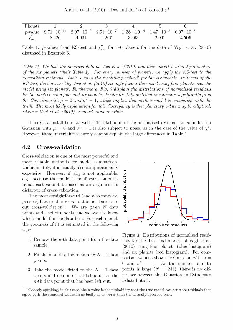
Table 1). We take the identical data as Vogt et al. (2010) and their asserted orbital parametersof the six planets (their Table 2). For every number of planets, we apply the KS-test to thenormalised residuals. Table 1 gives the resulting p-values9 for the six models. In terms of theKS-test, the data used by Vogt et al. (2010) strongly favour the model using four planets over themodel using six planets. Furthermore, Fig. 3 displays the distributions of normalised residualsfor the models using four and six planets. Evidently, both distributions deviate significantly fromthe Gaussian with µ = 0 and σ2 = 1, which implies that neither model is compatible with thetruth. The most likely explanation for this discrepancy is that planetary orbits may be elliptical,whereas Vogt et al. (2010) assumed circular orbits.

There is a pitfall here, as well. The likelihood of the normalised residuals to come from aGaussian with µ = 0 and σ2 = 1 is also subject to noise, as in the case of the value of χ2.However, these uncertainties surely cannot explain the large differences in Table 1.

4.2 Cross-validation

Figure 3: Distributions of normalised resid-uals for the data and models of Vogt et al.(2010) using four planets (blue histogram)and six planets (red histogram). For com-parison we also show the Gaussian with µ =0 and σ2 = 1. As the number of datapoints is large (N = 241), there is no dif-ference between this Gaussian and Student’st-distribution.

Cross-validation is one of the most powerful andmost reliable methods for model comparison.Unfortunately, it is usually also computationallyexpensive. However, if χ2

red is not applicable,e.g., because the model is nonlinear, computa-tional cost cannot be used as an argument indisfavour of cross-validation.

The most straightforward (and also most ex-pensive) flavour of cross-validation is “leave-one-out cross-validation”. We are given N datapoints and a set of models, and we want to knowwhich model fits the data best. For each model,the goodness of fit is estimated in the followingway:

1. Remove the n-th data point from the datasample.

2. Fit the model to the remaining N −1 datapoints.

3. Take the model fitted to the N − 1 datapoints and compute its likelihood for then-th data point that has been left out.

9Loosely speaking, in this case, the p-value is the probability that the true model can generate residuals thatagree with the standard Gaussian as badly as or worse than the actually observed ones.

9


4. Repeat steps 1 to 3 from n = 1 to n = Nand compute the goodness of the predic-tion of the whole data set by multiplyingthe likelihoods obtained in step 3.

Steps 3 and 4 require the data’s error distribution to be known in order to evaluate the good-ness of the prediction for the left-out data point through its likelihood. For instance, if thedata’s errors are Gaussian, the goodness of the prediction is simply given by Eq. (13) asusual. Evidently, repeating steps 1 to 3 N times is what makes leave-one-out cross-validationcomputationally expensive. It is also possible to leave out more than one data point in eachstep.10 However, if the given data set is very small, cross-validation becomes unstable. A niceapplication of cross-validation can be found, e.g., in Hogg (2008).

4.3 Bootstrapping

Bootstrapping is somewhat more general than cross-validation, meaning it requires less knowl-edge about the origin of the data. Cross-validation requires the data’s error distribution to beknown in order to evaluate the likelihoods, whereas bootstrapping does not. Of course, this isan advantage if we do not have this knowledge. However, if we do know the data’s errors, weshould definitely exploit this knowledge by using cross-validation. Bootstrapping is discussedin Andrae (2010) in the context of error estimation. Therefore, we restrict its discussion hereon the context of model comparison.

Let us suppose we are given 4 measurements y1, y2, y3, y4. We then draw subsamples ofsize 4 from this data set with replacement. These subsamples are called bootstrap samples.Examples are:

• y1, y2, y3, y4 itself,

• y1, y2, y2, y4,

• y2, y4, y4, y4,

• y1, y1, y1, y1,

• etc.

We draw a certain number of such bootstrap samples, and to every such sample we then fit allthe models that are to be compared.

In the context of model comparison, bootstrapping is typically used as “leave-one-out boot-strap” (e.g. Hastie et al. 2009). The algorithm is given by:

1. Draw a certain number of bootstrap samples from a given data set.

2. Fit all the models to every bootstrap sample.

3. For the n-th data point yn in the given data set, consider only those bootstrap samplesthat do not contain yn. Predict yn from the models fitted to these bootstrap samples.

4. Repeat step 3 from n = 1 to n = N and monitor the goodness of the predictions, e.g., byleast squares.

Like cross-validation, bootstrapping aims at the prediction error of the model. Therefore, it issensitive to over- and underfittings.

10The reason why cross-validation is so reliable is that it draws on the predictive error of the model, ratherthan the fitting error. Therefore, cross-validation can detect underfitting (the model is not flexible enough todescribe the data) and also overfitting (the model is too flexible compared to the data). The fitting error is onlysensitive to underfitting, but not to overfitting (χ2 always decreases if the model becomes more complex).

10


5 Conclusions

We have argued that there are two fundamental problems in using χ2red, which are completely

independent of each other:

1. In Sect. 2, we have seen that estimating the number of degrees of freedom, which isnecessary for evaluating χ2

red, is absolutely nontrivial in practice:

• Concerning linear models, for N given data points and P fit parameters the numberof degrees of freedom is somewhere between N − P and N − 1, where it is N − P ifand only if the basis functions of the linear model are linearly independent for thegiven data. Equation (8) provides a quantification for the effective number of fitparameters of a linear model. Priors can cause a linear model to become nonlinear.

• Concerning nonlinear models, the number of degrees of freedom is somewhere be-tween zero and N − 1 and it may not even be constant during a fit, i.e., N − P is acompletely unjustified guess. The authors are not aware of any method that reliablyestimates the number of degrees of freedom for nonlinear models. Consequently, itappears to be impossible to compute χ2

red in this case.

2. In Sect. 3, we have seen that the actual value of χ2red is uncertain. If the number N of

given data points is large, the uncertainty of χ2red is approximately given by the Gaussian

error σ =√

2/N . For N = 1, 000 data points, this means that within the 3σ-interval0.865 ≤ χ2

red ≤ 1.135 we cannot compare models or assess convergence.

Given these considerations, it appears highly questionable whether the popularity of χ2red –

which is certainly due to its apparent simplicity – is indeed justified. As a matter of fact, χ2red

cannot be evaluated for a nonlinear model, because the number of degrees of freedom is unknownin this case. This is a severe restriction, because many relevant models are nonlinear. Moreover,even for linear models, χ2

red has to be used with due caution, considering the uncertainty in itsvalue.

Concerning alternative methods for model comparison, we have explained cross-validationand bootstrapping in Sect. 4. We also explained how the normalised residuals of a model can beused to infer how close this model is to the true model underlying the given data. Concerningalternative methods for error estimation, we refer the interested reader to Andrae (2010).

Finally, we want to emphasise that the above considerations concerning χ2red have no impact

on the correctness of minimising a χ2 in order to fit a model to data. Fitting models to data isa completely different task that should not be confused with model comparison or convergencetesting. Minimising χ2 is the correct thing to do whenever the data’s measurement errors areGaussian and a maximum-likelihood estimate is desired.

Acknowledgements RA thanks David Hogg for detailed discussions on this subject. DavidHogg also came up with a couple of the examples mentioned here. Furthermore, RA thanksCoryn Bailer-Jones for helpful comments on the contents of this manuscript. RA is funded bya Klaus-Tschira scholarship. TS is funded by a grant from the Max Planck Society. PM issupported by the DFG Priority Programme 1177.

References

Andrae, R. 2010, ArXiv e-prints 1009.2755

Barlow, R. 1993, Statistics: A Guide to the Use of Statistical Methods in the Physical Sciences(Wiley VCH)

11


Hastie, T., Tibshirani, R., & Friedman, J. 2009, The Elements of Statistical Learning: DataMining, Inference, and Prediction. (Springer-Verlag)

Hogg, D. W. 2008, ArXiv e-prints 0807.4820

Kolmogorov, A. 1933, Giornale dell’ Istituto Italiano degli Attuari, 4, 83

Mayor, M., Bonfils, X., Forveille, T., et al. 2009, A&A, 507, 487

Smirnov, N. 1948, Annals of Mathematical Statistic, 19, 279

Vogt, S. S., Butler, R. P., Rivera, E. J., et al. 2010, ApJ, 723, 954

Ye, J. 1998, Journal of the American Statistical Association, 93, 120

12

dos and don’ts of reduced chi-squared - arxiv.org e ... · pdf filedos and don’ts...

Documents