Des outils pour l’adaptationde maillage anisotrope en
dimension 2 et 3F. Hecht
Laboratoire Jacques-Louis Lions
Universite Pierre et Marie Curie
Paris, France
http://www.ann.jussieu.fr/~hecht mailto:[email protected]
Cermics, Novembre, 2003 1
PLAN
– Introduction
– un schema d’adaptation
– Metrique et Maillage unite
– Outil lie aux metriques
– intersection, interpolation, gradation
– Metrique versu indicateur d’erreur
– Metrique pour element fini P1
– Metrique pour element fini P2
– Probleme de convergence (pas le temps)
– http://www.ann.jussieu.fr/~hecht/freefem++.htm
– Exemples / Demo of FreeFem++
– Conclusion / Future (pas le temps)
Cermics, Novembre, 2003 2
Introduction : Le vrai probleme
Nous voulons resoudre une EDP, dans un domain Ω avec la methode des
elements finis,
Le plus vite possible avec une precision donnee ε.
The theorie of error indicator given, the level of the error, but how to
compute the local mesh size to get a equidistribuate error.
Cermics, Novembre, 2003 3
Scheme of mesh adaption
i=0 ;
Soit Thi initial mesh
loop
compute ui the solution on mesh Thi
evaluate the level of error ε
si ε < ε0 break
compute the new local mesh size
construct a mesh according to prescribe the mesh size.
Remarque : comment transforme un indicateur d’erreur local ηK en carte de
taille. Moralement, il faut estimer :
∂ηK
∂hi
Cermics, Novembre, 2003 4
A main IDEA
– The difficulty is to find a tradeoff between the error estimate and the mesh
generation, because this two work are strongly different.
– To do that, we propose way based on a metric M and unit mesh w.r.t M– The metric is a way to control the mesh size.
– remark : The class of the mesh which can be created by the metric, is very
large.
Cermics, Novembre, 2003 5
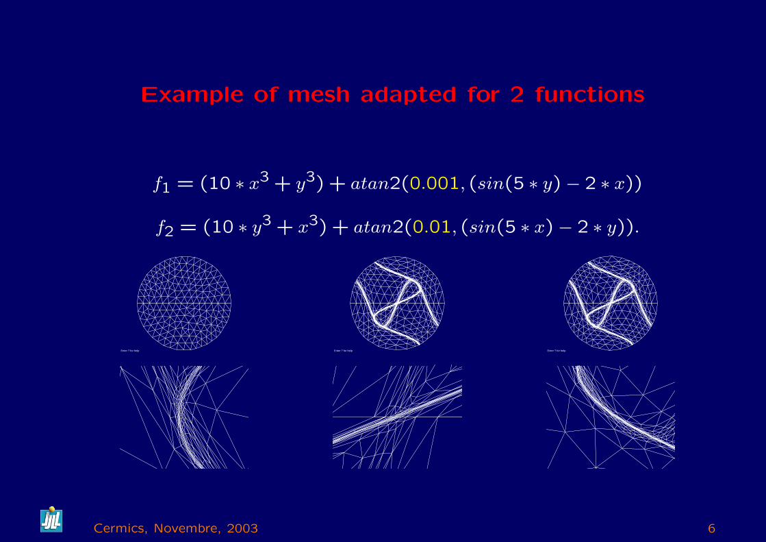
Example of mesh adapted for 2 functions
f1 = (10 ∗ x3 + y3) + atan2(0.001, (sin(5 ∗ y)− 2 ∗ x))
f2 = (10 ∗ y3 + x3) + atan2(0.01, (sin(5 ∗ x)− 2 ∗ y)).
Enter ? for help Enter ? for help Enter ? for help
Cermics, Novembre, 2003 6
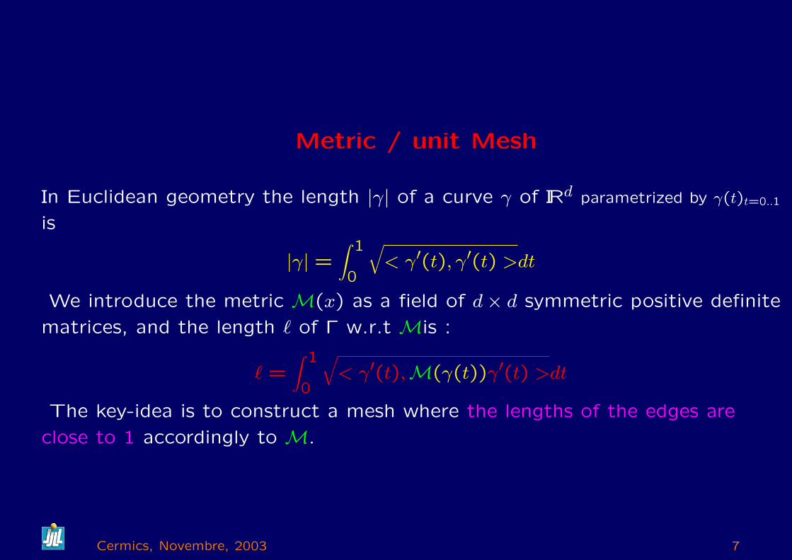
Metric / unit Mesh
In Euclidean geometry the length |γ| of a curve γ of IRd parametrized by γ(t)t=0..1
is
|γ| =∫ 1
0
√< γ′(t), γ′(t) >dt
We introduce the metric M(x) as a field of d× d symmetric positive definite
matrices, and the length ` of Γ w.r.t Mis :
` =∫ 1
0
√< γ′(t),M(γ(t))γ′(t) >dt
The key-idea is to construct a mesh where the lengths of the edges are
close to 1 accordingly to M.
Cermics, Novembre, 2003 7
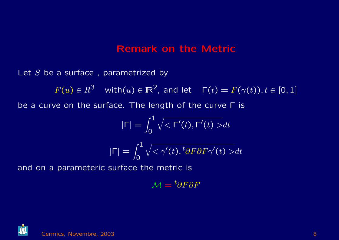
Remark on the Metric
Let S be a surface , parametrized by
F (u) ∈ R3 with(u) ∈ IR2, and let Γ(t) = F (γ(t)), t ∈ [0,1]
be a curve on the surface. The length of the curve Γ is
|Γ| =∫ 1
0
√< Γ′(t),Γ′(t) >dt
|Γ| =∫ 1
0
√< γ′(t), t∂F∂Fγ′(t) >dt
and on a parameteric surface the metric is
M = t∂F∂F
Cermics, Novembre, 2003 8
the Metric versus mesh size
at a point P ,
M =
(a bb c
)
M = R(
λ1 00 λ2
)R−1
where R = (v1, v2) is the matrix construct with the 2 unit eigenvectors vi and
λ1, λ2 the 2 eigenvalues.
The mesh size hi in direction vi is given by 1/√
λi
λi =1
h2i
Cermics, Novembre, 2003 9
Remark on metric :
If the metric is independant of position, then geometry is euclidian. But the
circle in metric become ellipse in classical space.
Infact, the unit ball (ellipse) in a metric given the mesh size in all the
direction, because the size of the edge of mesh is close to 1 the metric.
If the metric is dependant of the position, then you can speak about
Riemmanian geometry, and in this case the sides of triangle are geodesics,
but the case of mesh generation, you want linear edge.
Cermics, Novembre, 2003 10
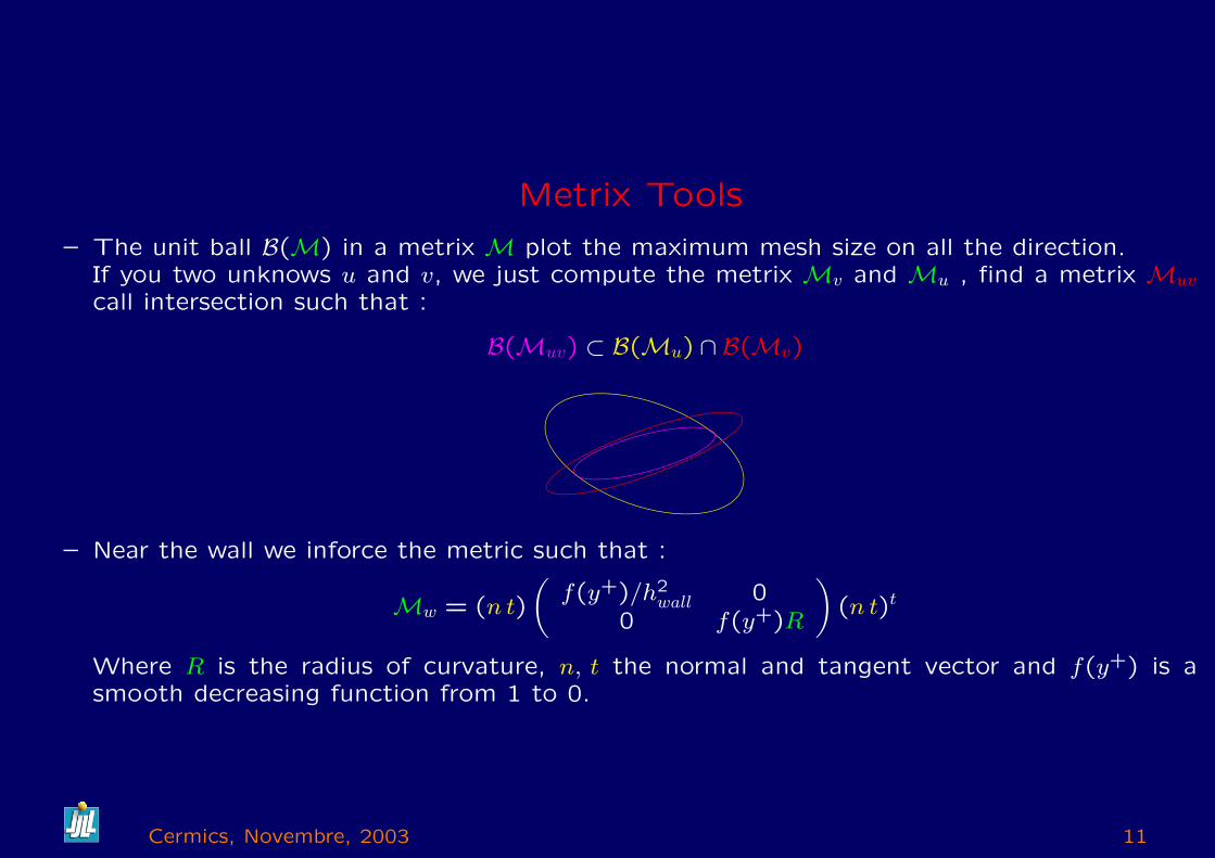
Metrix Tools
– The unit ball B(M) in a metrix M plot the maximum mesh size on all the direction.If you two unknows u and v, we just compute the metrix Mv and Mu , find a metrix Muv
call intersection such that :
B(Muv) ⊂ B(Mu) ∩ B(Mv)
– Near the wall we inforce the metric such that :
Mw = (n t)
(f(y+)/h2
wall 00 f(y+)R
)(n t)t
Where R is the radius of curvature, n, t the normal and tangent vector and f(y+) is asmooth decreasing function from 1 to 0.
Cermics, Novembre, 2003 11
Interpolation de Metric
– Generalement, la Metrique, n’est connue qu’aux sommets du maillage, il
faut donc interpole.
– l’interpolation direct des matrices (revient a dire que la fonction est P3 (on
genere trop de points).
– l’iterpolation en h revient a interpole avec
M(t) =((t)M−1
2A + (1− t)M−1
2B
)−2
car 1/h2 ∼ λ (trop lent)
– une derniere solution est :
M(t) =((t)M−1
A + (1− t)M−1B
)−1
Cermics, Novembre, 2003 12
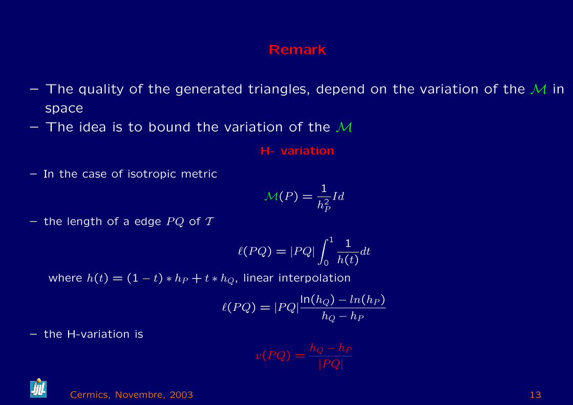
Remark
– The quality of the generated triangles, depend on the variation of the M in
space
– The idea is to bound the variation of the M
H- variation
– In the case of isotropic metric
M(P ) =1
h2P
Id
– the length of a edge PQ of T
`(PQ) = |PQ|∫ 1
0
1
h(t)dt
where h(t) = (1− t) ∗ hP + t ∗ hQ, linear interpolation
`(PQ) = |PQ|ln(hQ)− ln(hP)
hQ − hP
– the H-variation is
v(PQ) =hQ − hP
|PQ|
Cermics, Novembre, 2003 13
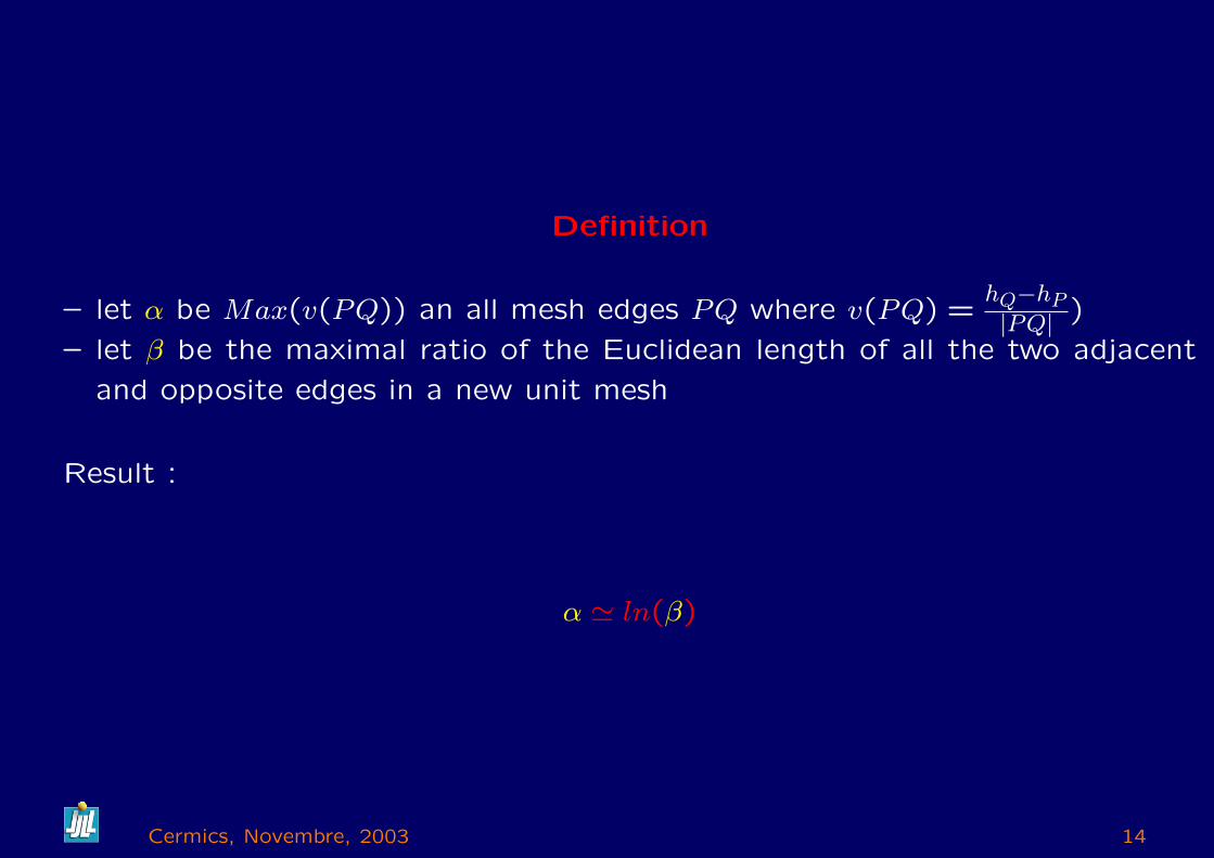
Definition
– let α be Max(v(PQ)) an all mesh edges PQ where v(PQ) =hQ−hP|PQ| )
– let β be the maximal ratio of the Euclidean length of all the two adjacent
and opposite edges in a new unit mesh
Result :
α ' ln(β)
Cermics, Novembre, 2003 14
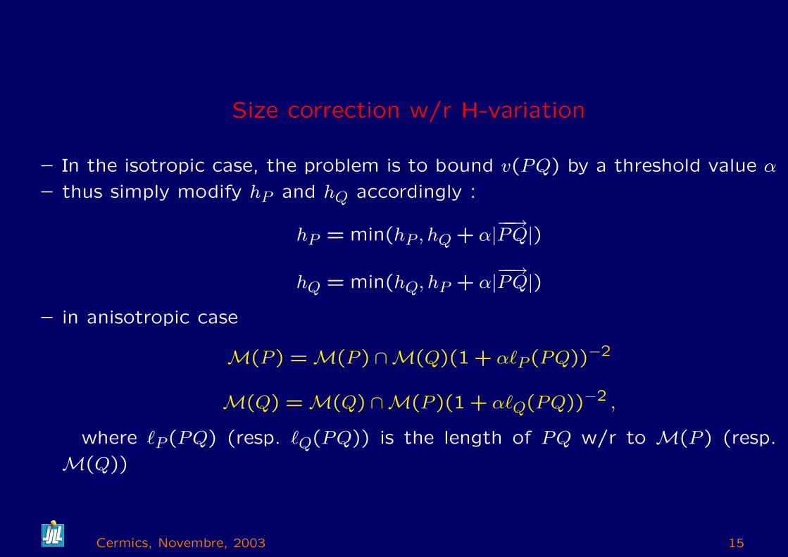
Size correction w/r H-variation
– In the isotropic case, the problem is to bound v(PQ) by a threshold value α
– thus simply modify hP and hQ accordingly :
hP = min(hP , hQ + α|−−→PQ|)
hQ = min(hQ, hP + α|−−→PQ|)
– in anisotropic case
M(P ) = M(P ) ∩M(Q)(1 + α`P (PQ))−2
M(Q) = M(Q) ∩M(P )(1 + α`Q(PQ))−2 ,
where `P (PQ) (resp. `Q(PQ)) is the length of PQ w/r to M(P ) (resp.
M(Q))
Cermics, Novembre, 2003 15
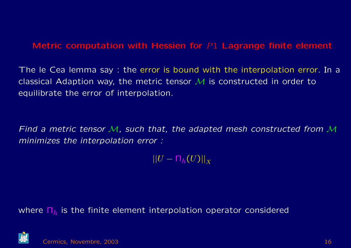
Metric computation with Hessien for P1 Lagrange finite element
The le Cea lemma say : the error is bound with the interpolation error. In a
classical Adaption way, the metric tensor M is constructed in order to
equilibrate the error of interpolation.
Find a metric tensor M, such that, the adapted mesh constructed from Mminimizes the interpolation error :
||U −Πh(U)||X
where Πh is the finite element interpolation operator considered
Cermics, Novembre, 2003 16
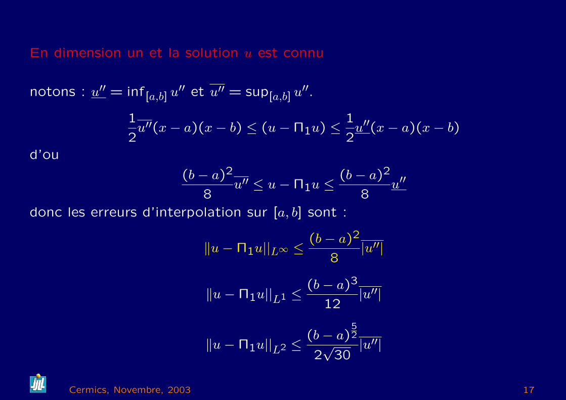
En dimension un et la solution u est connu
notons : u′′ = inf[a,b] u′′ et u′′ = sup[a,b] u
′′.
1
2u′′(x− a)(x− b) ≤ (u−Π1u) ≤
1
2u′′(x− a)(x− b)
d’ou
(b− a)2
8u′′ ≤ u−Π1u ≤
(b− a)2
8u′′
donc les erreurs d’interpolation sur [a, b] sont :
‖u−Π1u||L∞ ≤(b− a)2
8|u′′|
‖u−Π1u||L1 ≤(b− a)3
12|u′′|
‖u−Π1u||L2 ≤(b− a)
52
2√
30|u′′|
Cermics, Novembre, 2003 17
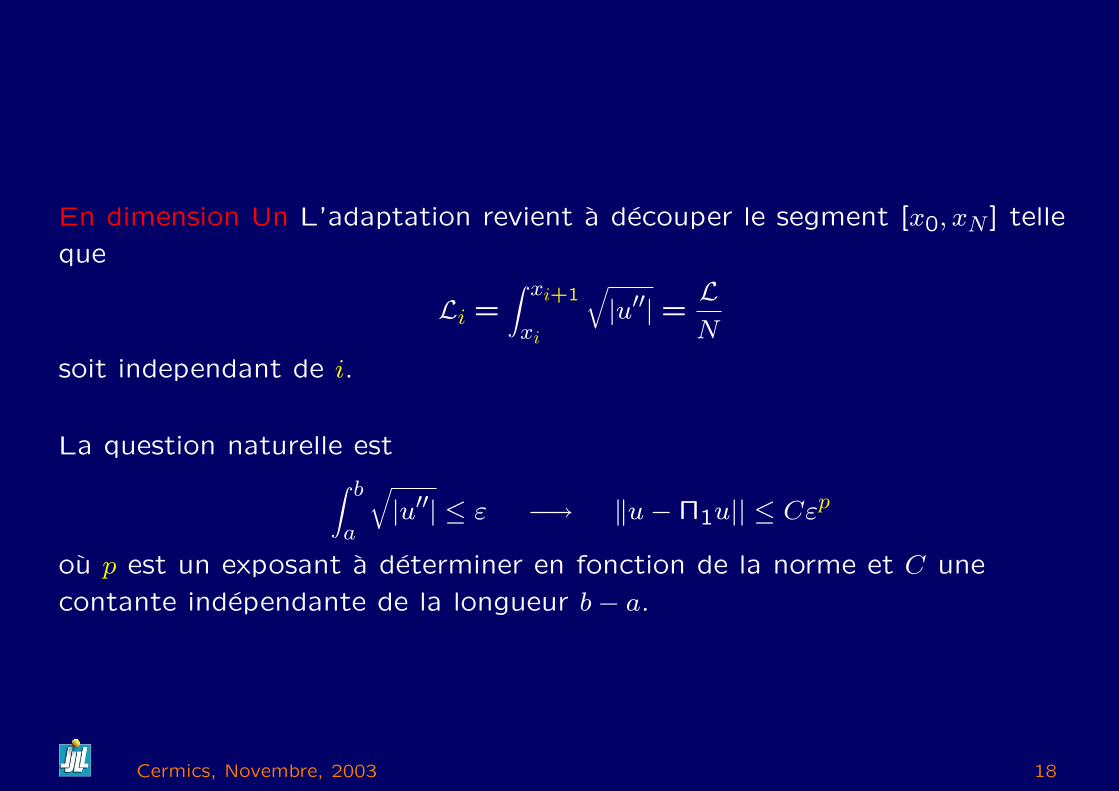
En dimension Un L’adaptation revient a decouper le segment [x0, xN ] telle
que
Li =∫ xi+1
xi
√|u′′| =
LN
soit independant de i.
La question naturelle est∫ b
a
√|u′′| ≤ ε −→ ‖u−Π1u|| ≤ Cεp
ou p est un exposant a determiner en fonction de la norme et C une
contante independante de la longueur b− a.
Cermics, Novembre, 2003 18
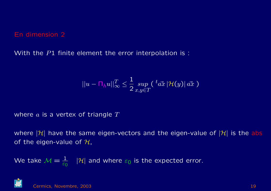
En dimension 2
With the P1 finite element the error interpolation is :
||u−Πhu||T∞ ≤1
2sup
x,y∈T( t ~ax |H(y)| ~ax )
where a is a vertex of triangle T
where |H| have the same eigen-vectors and the eigen-value of |H| is the abs
of the eigen-value of H,
We take M = 1ε0
|H| and where ε0 is the expected error.
Cermics, Novembre, 2003 19
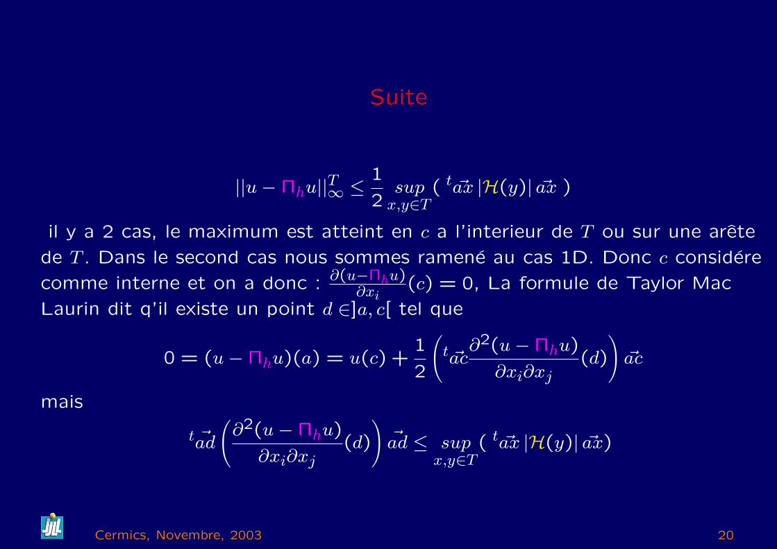
Suite
||u−Πhu||T∞ ≤1
2sup
x,y∈T( t ~ax |H(y)| ~ax )
il y a 2 cas, le maximum est atteint en c a l’interieur de T ou sur une arete
de T . Dans le second cas nous sommes ramene au cas 1D. Donc c considere
comme interne et on a donc : ∂(u−Πhu)∂xi
(c) = 0, La formule de Taylor Mac
Laurin dit q’il existe un point d ∈]a, c[ tel que
0 = (u−Πhu)(a) = u(c) +1
2
(t ~ac
∂2(u−Πhu)
∂xi∂xj(d)
)~ac
mais
t ~ad
(∂2(u−Πhu)
∂xi∂xj(d)
)~ad ≤ sup
x,y∈T( t ~ax |H(y)| ~ax)
Cermics, Novembre, 2003 20
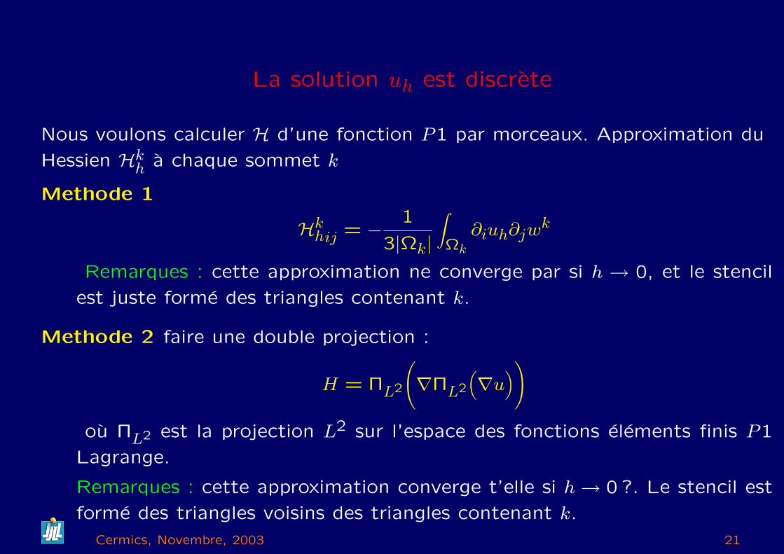
La solution uh est discrete
Nous voulons calculer H d’une fonction P1 par morceaux. Approximation du
Hessien Hkh a chaque sommet k
Methode 1
Hkhij = −
1
3|Ωk|
∫Ωk
∂iuh∂jwk
Remarques : cette approximation ne converge par si h → 0, et le stencil
est juste forme des triangles contenant k.
Methode 2 faire une double projection :
H = ΠL2
(∇ΠL2
(∇u
))
ou ΠL2 est la projection L2 sur l’espace des fonctions elements finis P1
Lagrange.
Remarques : cette approximation converge t’elle si h → 0 ?. Le stencil est
forme des triangles voisins des triangles contenant k.
Cermics, Novembre, 2003 21
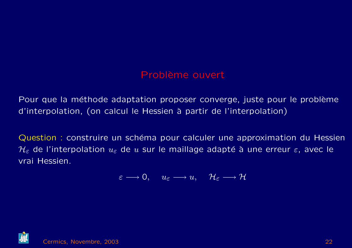
Probleme ouvert
Pour que la methode adaptation proposer converge, juste pour le probleme
d’interpolation, (on calcul le Hessien a partir de l’interpolation)
Question : construire un schema pour calculer une approximation du Hessien
Hε de l’interpolation uε de u sur le maillage adapte a une erreur ε, avec le
vrai Hessien.
ε −→ 0, uε −→ u, Hε −→ H
Cermics, Novembre, 2003 22
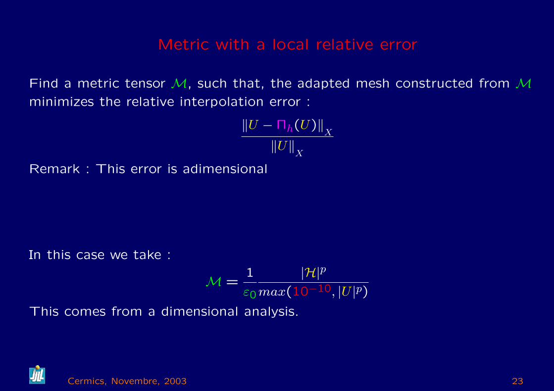
Metric with a local relative error
Find a metric tensor M, such that, the adapted mesh constructed from Mminimizes the relative interpolation error :
‖U −Πh(U)‖X
‖U‖X
Remark : This error is adimensional
In this case we take :
M =1
ε0
|H|p
max(10−10, |U |p)This comes from a dimensional analysis.
Cermics, Novembre, 2003 23
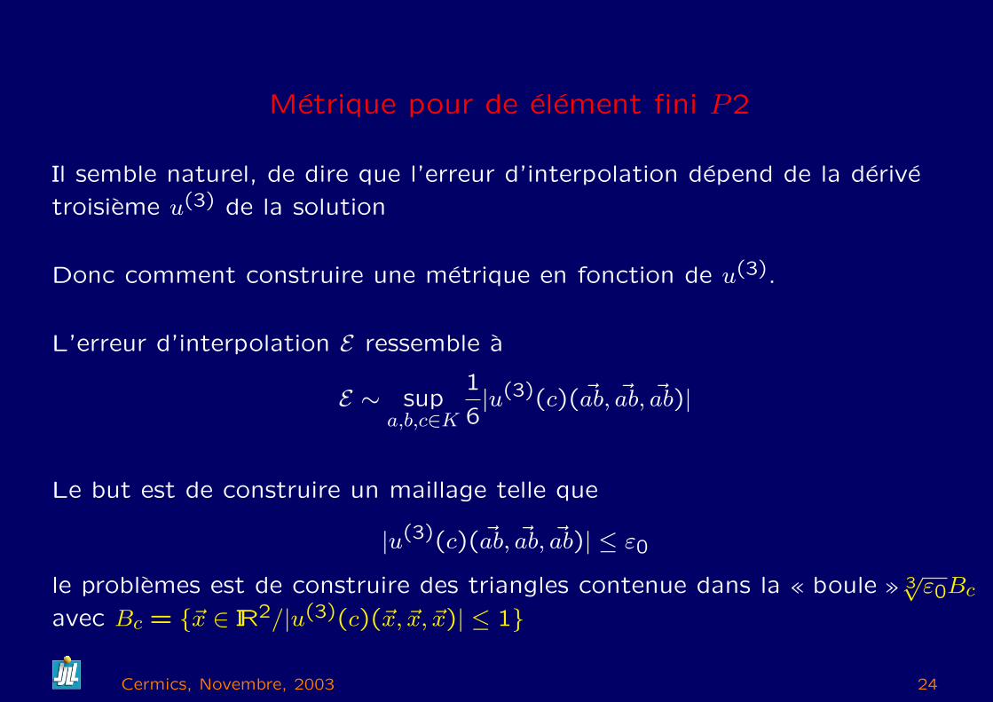
Metrique pour de element fini P2
Il semble naturel, de dire que l’erreur d’interpolation depend de la derive
troisieme u(3) de la solution
Donc comment construire une metrique en fonction de u(3).
L’erreur d’interpolation E ressemble a
E ∼ supa,b,c∈K
1
6|u(3)(c)( ~ab, ~ab, ~ab)|
Le but est de construire un maillage telle que
|u(3)(c)( ~ab, ~ab, ~ab)| ≤ ε0
le problemes est de construire des triangles contenue dans la « boule » 3√
ε0Bc
avec Bc = ~x ∈ IR2/|u(3)(c)(~x, ~x, ~x)| ≤ 1
Cermics, Novembre, 2003 24
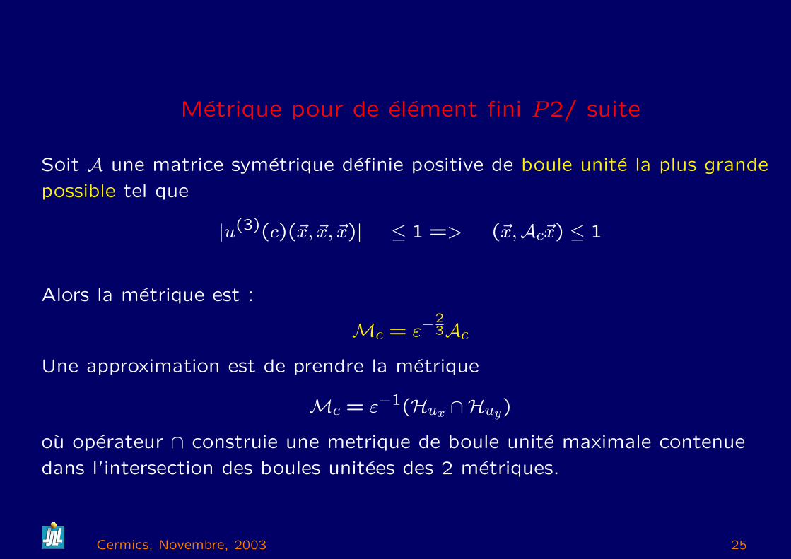
Metrique pour de element fini P2/ suite
Soit A une matrice symetrique definie positive de boule unite la plus grande
possible tel que
|u(3)(c)(~x, ~x, ~x)| ≤ 1 => (~x,Ac~x) ≤ 1
Alors la metrique est :
Mc = ε−23Ac
Une approximation est de prendre la metrique
Mc = ε−1(Hux ∩Huy)
ou operateur ∩ construie une metrique de boule unite maximale contenue
dans l’intersection des boules unitees des 2 metriques.
Cermics, Novembre, 2003 25
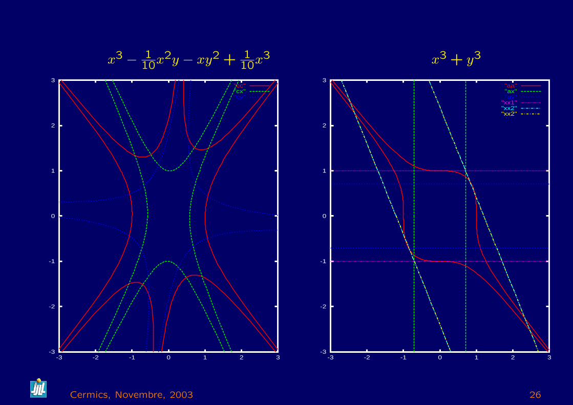
x3 − 110x2y − xy2 + 1
10x3 x3 + y3
-3
-2
-1
0
1
2
3
-3 -2 -1 0 1 2 3
"cc""cx""cy"
-3
-2
-1
0
1
2
3
-3 -2 -1 0 1 2 3
"aa""ax""ay"
"xx1""xx2""xx2"
Cermics, Novembre, 2003 26
Conclusion
Les metriques sont une methode tres puissantes pour faire de l’adaptation de
maillage.
Mais, il y a un manque de support mathematique.
Probleme ouvert :
Trouver de bons schemas pour calculer le Hessien.
Cermics, Novembre, 2003 27
Logiciel sur la Toile
In the directoryftp://ftp.inria.fr/INRIA/Projects/Gamma/ on INTERNET :
– 2D CAD+ mesh generator :Emc2.tar.gzwritten in f77 translated in C
– 2D adaption loopbamg.tar.gzwritten in C++
– 2D Compressible Navier Stokes solverwritten in F77NSC2KE.tar.gz
– FreeFem++ : a 2D PDE solvehttp ://www.ann.jussieu.fr/ hecht/freefem++.htm
Cermics, Novembre, 2003 28


