
1
EIT Waves: A Changing Understanding over a Solar Cycle M. J. Wills-Davey and G. D. R. Attrill
Smithsonian Astrophysical Observatory, 60 Garden St., Cambridge, MA, 01238, USA +1-617-495-7852
+1-617-496-7577
EIT waves were first observed by SOHO-EIT in 1996. Careful analysis has shown that they are
related to many other phenomena including: Coronal Mass Ejections (CMEs), coronal dimming
regions, Moreton waves, and transverse coronal loop oscillations. Over the years, myriad theories
have been proposed to explain EIT waves. This has led to the coexistence of competing models,
some of which contradict each other. Sifting through these models requires a thorough
understanding of the available data, as some observations make certain theories more difficult to
justify. In fact, some questions do not appear to be resolvable with current data. We eagerly
anticipate the next generation of coronal telescopes, which will dramatically assist us in
conclusively determining the true nature of EIT waves.
Sun: corona, EIT waves—Waves—MHD
AIA: Atmospheric Imaging Assembly;
CME: Coronal Mass Ejection;
EIT: Extreme-ultraviolet Image Telescope;
EUV: extreme ultraviolet;
EUVI: Extreme UltraViolet Imager;
MHD: magnetohydrodynamic;
SDO: Solar Dynamics Observatory;
SOHO: Solar and Heliospheric Observatory;
SECCHI: Sun Earth Connection Coronal and Heliospheric Investigation;
STEREO: Solar TErrestrial RElations Observatory;
SXT: Soft X-ray Telescope;
TRACE: Transition Region and Coronal Explorer;
XRT: X-Ray Telescope
2
1 Introduction
Although only discovered a little over a decade ago (Dere et al. 1997), large-scale, diffuse, single-
pulse coronal propagating fronts have rapidly become part of the heliophysics lexicon. Although
known colloquially as “EIT waves”—recognizing their initial discovery by the SOHO-EIT
instrument (Delaboudiniere et al. 1995)—it is important to note that the label “wave” is purely
phenomenological; while in many respects they act like waves, several recent models question this
assumption, and put forth alternative theories. This review will discuss the many observations and
various current models for understanding coronal EIT waves. Warmuth et al. (2005) states that
“probably a considerable fraction of coronal transients are not really waves at all…[This] poses a
problem for their use as tools for deriving ambient coronal parameters, which require the
disturbances to be MHD waves.” (e.g. Mann et al. (1999); Ballai and Erdélyi (2004); Ballai et al.
(2005); Warmuth et al. (2005); Warmuth and Mann (2005). Before analysis of coronal wave
behavior can be confidently utilized for coronal seismology, clarification concerning the physics
behind the various types of wave-like phenomena is required.
Part of the reason for the debate regarding the status of the physical nature of EIT waves is the
various difficulties concerning their observation. Until the recent launch of STEREO (Kaiser
2005), EIT waves were only observed by the TRACE (Handy et al. 1999) and EIT telescopes.
Such observations are problematic for two main reasons: (1) the ~12-18 minute cadence and single
(195 Å) passband of the EIT “CME Watch” limits the number of frames and passbands in which
these events can be viewed, and (2) the limited TRACE field-of-view (8′ x 8′) constrains the
viewable range of any passing EIT wave, decreasing the number and extent of recorded events.
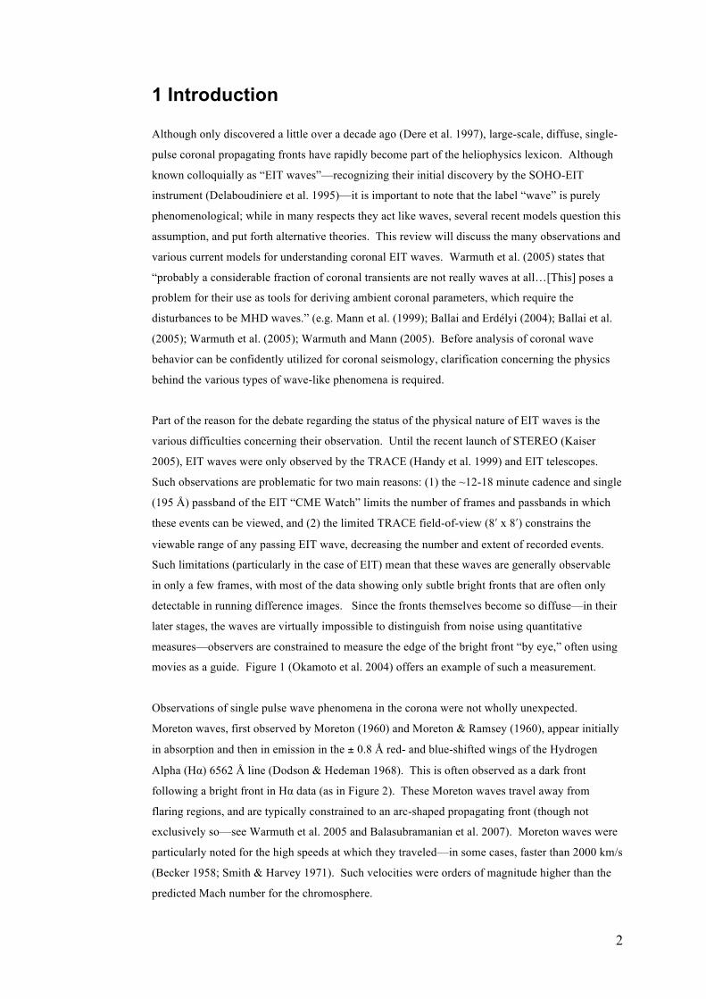
Such limitations (particularly in the case of EIT) mean that these waves are generally observable
in only a few frames, with most of the data showing only subtle bright fronts that are often only
detectable in running difference images. Since the fronts themselves become so diffuse—in their
later stages, the waves are virtually impossible to distinguish from noise using quantitative
measures—observers are constrained to measure the edge of the bright front “by eye,” often using
movies as a guide. Figure 1 (Okamoto et al. 2004) offers an example of such a measurement.
Observations of single pulse wave phenomena in the corona were not wholly unexpected.
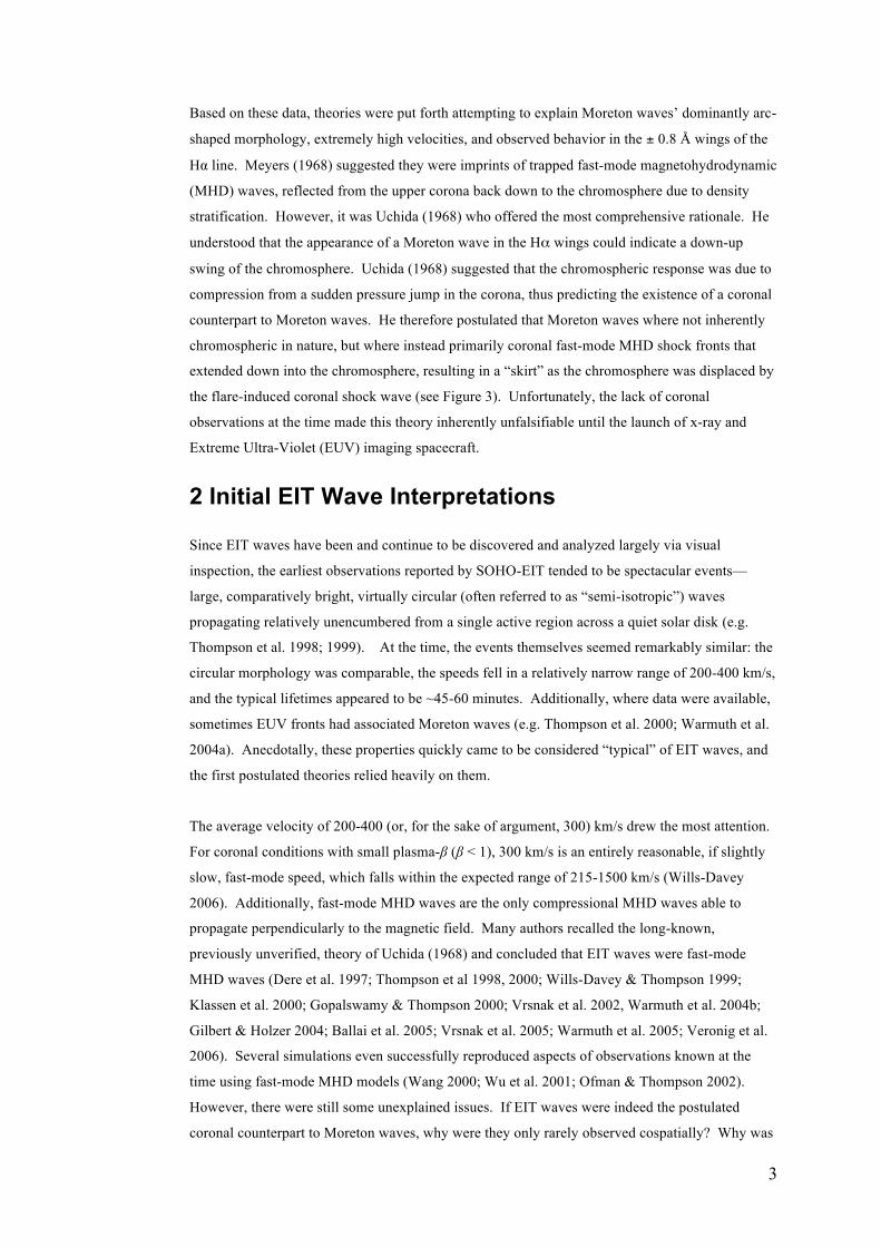
Moreton waves, first observed by Moreton (1960) and Moreton & Ramsey (1960), appear initially
in absorption and then in emission in the ± 0.8 Å red- and blue-shifted wings of the Hydrogen
Alpha (Hα) 6562 Å line (Dodson & Hedeman 1968). This is often observed as a dark front
following a bright front in Hα data (as in Figure 2). These Moreton waves travel away from
flaring regions, and are typically constrained to an arc-shaped propagating front (though not
exclusively so—see Warmuth et al. 2005 and Balasubramanian et al. 2007). Moreton waves were
particularly noted for the high speeds at which they traveled—in some cases, faster than 2000 km/s
(Becker 1958; Smith & Harvey 1971). Such velocities were orders of magnitude higher than the
predicted Mach number for the chromosphere.
3
Based on these data, theories were put forth attempting to explain Moreton waves’ dominantly arc-
shaped morphology, extremely high velocities, and observed behavior in the ± 0.8 Å wings of the
Hα line. Meyers (1968) suggested they were imprints of trapped fast-mode magnetohydrodynamic
(MHD) waves, reflected from the upper corona back down to the chromosphere due to density
stratification. However, it was Uchida (1968) who offered the most comprehensive rationale. He
understood that the appearance of a Moreton wave in the Hα wings could indicate a down-up
swing of the chromosphere. Uchida (1968) suggested that the chromospheric response was due to
compression from a sudden pressure jump in the corona, thus predicting the existence of a coronal
counterpart to Moreton waves. He therefore postulated that Moreton waves where not inherently
chromospheric in nature, but where instead primarily coronal fast-mode MHD shock fronts that
extended down into the chromosphere, resulting in a “skirt” as the chromosphere was displaced by
the flare-induced coronal shock wave (see Figure 3). Unfortunately, the lack of coronal
observations at the time made this theory inherently unfalsifiable until the launch of x-ray and
Extreme Ultra-Violet (EUV) imaging spacecraft.
2 Initial EIT Wave Interpretations
Since EIT waves have been and continue to be discovered and analyzed largely via visual
inspection, the earliest observations reported by SOHO-EIT tended to be spectacular events—
large, comparatively bright, virtually circular (often referred to as “semi-isotropic”) waves
propagating relatively unencumbered from a single active region across a quiet solar disk (e.g.
Thompson et al. 1998; 1999). At the time, the events themselves seemed remarkably similar: the
circular morphology was comparable, the speeds fell in a relatively narrow range of 200-400 km/s,
and the typical lifetimes appeared to be ~45-60 minutes. Additionally, where data were available,
sometimes EUV fronts had associated Moreton waves (e.g. Thompson et al. 2000; Warmuth et al.
2004a). Anecdotally, these properties quickly came to be considered “typical” of EIT waves, and
the first postulated theories relied heavily on them.
The average velocity of 200-400 (or, for the sake of argument, 300) km/s drew the most attention.
For coronal conditions with small plasma-β (β < 1), 300 km/s is an entirely reasonable, if slightly
slow, fast-mode speed, which falls within the expected range of 215-1500 km/s (Wills-Davey
2006). Additionally, fast-mode MHD waves are the only compressional MHD waves able to
propagate perpendicularly to the magnetic field. Many authors recalled the long-known,
previously unverified, theory of Uchida (1968) and concluded that EIT waves were fast-mode
MHD waves (Dere et al. 1997; Thompson et al 1998, 2000; Wills-Davey & Thompson 1999;
Klassen et al. 2000; Gopalswamy & Thompson 2000; Vrsnak et al. 2002, Warmuth et al. 2004b;
Gilbert & Holzer 2004; Ballai et al. 2005; Vrsnak et al. 2005; Warmuth et al. 2005; Veronig et al.
2006). Several simulations even successfully reproduced aspects of observations known at the
time using fast-mode MHD models (Wang 2000; Wu et al. 2001; Ofman & Thompson 2002).
However, there were still some unexplained issues. If EIT waves were indeed the postulated
coronal counterpart to Moreton waves, why were they only rarely observed cospatially? Why was
4
the morphology of most EIT waves (~93%; Biesecker et al. 2002) broad and diffuse, unlike the
sharp, arc-shaped shock fronts observed in the chromosphere? Why were the observed velocities
so much slower (typically by a factor of two or three) than those associated with Moreton waves?
To account for these discrepancies, variations on the Uchida (1968) model were suggested.
Warmuth et al. (2004a,b) postulated that EIT waves really were the coronal counterparts of
Moreton waves; one just needed to account for deceleration. Using curved, rather than linear, fits,
they were able to account for the motion of several events and resolve the discrepancy between the
two wave velocities (see Figure 4).
As an alternate theory, Chen et al. (2002, 2005) developed a numerical model, building on work
by Delannée & Aulanier (1999), who argued that EIT bright fronts were not true “waves” at all,
but instead features caused by compression. In the Chen et al. (2002, 2005) simulations, a flux
rope erupts, gradually “opening” the overlying magnetic field. The opening-related deformation is
transferred from the top to the footpoint of each field line overlying the flux rope, so that EIT
“wave” bright fronts are formed successively, creating a propagating plasma enhancement. Such
an eruption would be expected to generate both a Moreton wave—a fast-mode MHD shock, which
would quickly propagate away—and a much slower EIT wave—not a true “wave” in the physical
sense, but an expanding bright front generated as a result of density enhancements at the footpoints
of successively larger overlying field lines. Functionally, EIT waves, in this model, could be
described as wave-like “wakes” behind Moreton waves. This model not only reproduces the slow
velocity of EIT waves, but also accounts for their broad, diffuse nature.
The models discussed above, albeit dramatically different as wave and non-wave interpretations
respectively, do an excellent job of explaining the aforementioned “typical” properties of EIT
waves: they account for velocities of ~300 km/s, they couple EIT waves to Moreton waves, and
they explain the velocity differences between the two phenomena. However, as analysis and
observations have multiplied and improved over time, these “typical” EIT wave attributes turn out
to not be as representative as previously thought. In fact, each of these assumptions can be tracked
back to two very influential items: the EIT “CME Watch” cadence, and the study of well-defined
events, rather than a more “representative” sample.1
When considered objectively, the ~12-18 minute EIT “CME Watch” 195 Å cadence, by its nature,
must introduce certain bias. Since EIT waves are identified almost exclusively in difference
images, the lifetime necessary to appear in even one differenced frame is >12-18 minutes.
Additionally, as EIT waves are dynamic, often several frames are necessary to provide enough
data to study; an event must last ~30 minutes to produce two measurable frames, ~45 minutes to
1 As, at present, only rudimentary software packages exist that can automatically identify EIT waves (Podladchikova and Berghmans 2005; Wills-Davey 2006), it is important to understand that all currently-studied EIT waves are ultimately viewer-identified. However, some studies (Biesecker et al. 2002; Wills-Davey et al. 2007; Thompson & Myers 2009) take pains to include less well-defined events, offering a larger range of results.
5
produce three measureable frames, and so on. This means that waves with lifetimes of >30-45
minutes are likely to be preferentially selected as subjects for study.
The requirement of such a long lifetime leads to additional constraints. Only the simplest large-
scale structures are likely to remain coherent for >30 minutes as they travel across the solar disk;
i.e. circular or semi-circular events tend to be most easily observed by SOHO-EIT. Additionally,
events that propagate at >500 km/s are difficult to observe in multiple “CME Watch” frames; such
fast waves are likely to travel over the limb, and, for all intents and purposes, their on-disk
“lifetimes” are too short to make them suitable for dynamic study. This provides an artificial
upper limit on the possible observed speeds of EIT waves.
A second important factor has also contributed to this “typical” definition of EIT waves: the
persistent analysis of a limited number of events, most notably those observed on by SOHO-EIT
on 12 May 1997 (e.g. Thompson et al. 1998; Wang 2000; Wu et al. 2001; Podladchikova &
Berghmans, 2005; Attrill et al. 2007a; Delannée et al. 2008) and 7 April 1997 (e.g. Thompson et
al. 1999; Wang 2000; Attrill et al. 2007a; Delannée et al. 2008). Both observers and modelers
have been drawn to these events for obvious reasons: they are well-defined, display relatively
simple morphology (due to their occurrence in the rise phase of solar cycle 23), and are well-
correlated with other energetic phenomena, such as CMEs and Type-II radio bursts.
There also exist a set of studies which were specifically interested in the possible connection
between EIT waves and Moreton waves (e.g. Thompson et al. 2000; Warmuth et al. 2001;
Pohjolainen et al. 2001; Khan and Aurass 2002; Eto et al. 2002; Warmuth et al. 2004a; Okomoto
et al. 2004; Temmer et al. 2005; Warmuth et al. 2005; Vrsnak et al. 2005; Veronig et al. 2006;
Delannée et al. 2007); therefore, their analyses are limited to events with definite Moreton wave
correlation. While a more extensive database of several hundred events has been compiled (B.
Thompson, private communication; Thompson & Myers 2009), only a small number of studies
considered the statistics of large numbers of recorded events (Biesecker et al. 2002; Cliver et al.
2005; Wills-Davey et al. 2007).
The nature of the earliest studies led to unintentional biases in language and understanding: the
large majority of early publications treated EIT waves as fast-mode MHD waves, and they were
regularly referred to as “coronal Moreton waves”. Such a name implied they were considered to
be flare-generated events, given the general consensus at the time regarding the initiation of
Moreton waves.
3 Observable Properties of EIT Waves
As time has gone on, and researchers have considered EIT waves—both their properties and their
physics—in greater detail, a new, more complex picture has emerged. In part, this is due to
additional observations from other EUV and x-ray instruments, such as TRACE, Yohkoh-SXT

6
(Tsuneta et al. 1991), SPIRIT (Zhitnik et al., 2002), GOES/SXI (Lemen et al. 2004), STEREO-
EUVI (Wülser et al. 2004), and Hinode-XRT (Golub et al. 2007). While no other instrument has
yet observed as many EIT waves as SOHO-EIT, such alternate data have provided improved
cadence, resolution, and temperature range. Ultimately, the accumulated data have shown that
scientists must take a great variety of characteristics into account when attempting to explain EIT
waves.
3.1 Morphology
While certain properties of EIT waves appear to vary greatly when individual events are
compared—they are alternatively global, contained; fast, slow; semi-isotropic, complex etc.—
certain morphological characteristics appear common to all observations. EIT waves are generally
described as single-pulse phenomena (a single expanding bright front). Although homologous
events are common, as yet, no observational evidence has been presented showing a “double” EIT
wave.2 In spite of mounting evidence in support of “double” (Neidig 2004; Gilbert et al. 2008) or
even “triple” Moreton waves (Narukage et al. 2008), and observations of multiple wave fronts in
He I data (Vrsnak et al. 2002; Gilbert & Holzer 2004; Gilbert et al. 2004) associated with EIT
wave events, current wavelet analysis of EUV data remains consistent with a single-pulse
explanation (Ballai et al. 2005; Wills-Davey et al. 2007).
Although a small number (~7%) of EIT observations display sharp, semi-circular wave fronts
early in a pulse’s lifetime (called “S-waves”; Biesecker et al. 2002 or “brow waves”; Gopalswamy
et al. 2000), and limited TRACE observations suggest that, early on, even non-“S waves” can
show strong definition (Wills-Davey 2006), the data show that all EIT waves eventually devolve
into broad, diffuse structures, with the bright front widths of order 100 Mm. This is not simply an
artifact of SOHO-EIT cadence, as evidenced by the higher-cadence TRACE and STEREO-EUVI
data (e.g. Wills-Davey 2006; Long et al. 2008). Such increasing diffuseness (Dere et al. 1997;
Thompson et al. 1999; Klassen et al. 2000; Podladchikova & Berghmans 2005) is consistent with
both flux conservation as the pulse expands away from its origin (Wills-Davey 2003) and with the
decay of a large-amplitude, semi-isotropic perturbation.
There is also mounting evidence that EIT waves are confined to a region 1-2 scale heights above
the chromosphere. Observations on the solar limb show most brightenings are observed within
several hundred Mm (Thompson et al. 1999; Warmuth et al. 2004a, 2005; Vrsnak et al. 2005).
Additionally, analytical calculations by Nye & Thomas (1976) and Wills-Davey (2003) find that
changes in Alfvén speed with altitude will result in the “trapping” of laterally-propagating MHD
waves below ~2 scale heights. Such findings are consistent with measurements by Wills-Davey
2 Dual brightenings have been reported for two EIT wave events by Attrill et al. (2007a), who show that a persistent brightening remains at the outermost edge of the deep, core dimming, while a propagating brightening forms simultaneously at the leading edge of the expanding bright front. In such a case, one brightening is stationary, while the other propagates.

7
(2003), who finds that, as the wave expands, flux drops off as r-1, rather than the r-2 expected for
spherical waves.
The bright fronts themselves are transitory features, with the front increasing the local intensity
over a period of a few minutes as the wave passes through. This is true even in high-cadence,
emission measure results available for some TRACE events (Wills-Davey 2003). Such transient
intensity increases imply some sort of temporary temperature or density enhancement.
Unfortunately, as most evidence of such behavior has so far been seen using EUV narrowband
filter detectors—such as those on SOHO-EIT, TRACE, and STEREO EUVI—is it difficult to de-
convolve temperature and density effects. It should be noted, though, that the observations
themselves provide certain constraints. Additionally, there do exist some observations of diffuse
coronal waves made by broadband x-ray imagers, namely GOES/SXI and Hinode/XRT (Warmuth
et al. 2005; Attrill et al. 2009, see Section 3.3).
Considerable evidence exists suggesting that EIT waves increase local density. Warmuth et al.
(2005) examine six diffuse bright front events, and see comparable morphology and brightness
increases from different filters across a large temperature range (1.5-4 MK); they conclude that
only compression could produce such observations. White & Thompson (2005) examine
contemporaneous EUV and radio data for an “S-wave” event, and find bright fronts in both. As
optically thin thermal free-free emission is only weakly temperature dependent (∝ T0.5), any
increase in radio emission is more likely due to density enhancement. By taking each passband as
isothermal (a poor estimate at best), Wills-Davey (2003, 2006) use automated methods to find
density enhancements caused by the 13 June 1998 front observed in TRACE data. Since emission
measure (EM) relates to density (ne) according to:
it is possible to derive density changes due to the event by using
Using these methods, Wills-Davey (2003, 2006) show extremely pronounced, non-linear density
enhancements early in the event lifetime (>40% above the background). Warmuth et al. (2004b)
find EIT observations consistent with similarly large enhancements, finding intensity
enhancements of up to 110% above the background.
While strong evidence for density enhancement exists, other results suggest heating is taking place
as well. Wills-Davey & Thompson (1999) observe a front in the TRACE data that appears bright
in the 195 Å passband, but dark in the corresponding 171 Å data. They claim this as evidence
that heating is occurring out of the 171 Å passband, which would be consistent with the plasma
(1)
(2)
8
temperature increasing from ~1 MK to ~1.4 MK. Gopalswamy & Thompson (2000) report similar
observational discrepancies in a multi-passband EIT observation.
The timescales of the subsequent cooling are particularly telling. Under quiet Sun conditions,
conductive cooling takes ~30 minutes, while radiative cooling times extend up to nine hours
(Wills-Davey 2003). If either mechanism was at work, heating due to EIT waves would be visible
for much more extended periods of time. This leads Wills-Davey (2003) to suggest that EIT wave
brightenings may be the result of thermal compression. The compression of plasma (density
increase) as well as heating are both invoked in the various models for coronal EIT waves.
3.2 Basic Dynamics
EIT waves are generally observed to be dynamic.3 Even smaller events tend to travel >1 R
through the lower corona (e.g. Thompson & Myers 2009), maintaining their coherence over global
distances. In each case, the bright front broadens and becomes less intense as it travels (e.g.
Klassen et al. 2000, Podladchikova & Berghmans 2005); this could be due to flux conservation
and possibly dispersion. There appears to be no evidence of periodicity as the bright front pulse
expands, with wavelet analysis showing the front encompassing a broad range of frequencies
(Ballai et al. 2005).
Published studies regarding the dispersion of EIT waves are inconclusive. Warmuth et al.
(2004a,b) visually consider eight events in the EIT “CME Watch” data and find evidence of
overall pulse width expansion, but do not measure σ. However, the single event measured by
Wills-Davey (2003) in high-cadence (~75 sec) TRACE data finds that, even though the pulse
width increases, σ remains constant at several points along the wave as it propagates, implying no
dispersion. Very recent work by Warmuth (A. Warmuth, private communication) uses more
quantitative methods, comparing σ as a function of propagation distance across multiple events in
SOHO-EIT and STEREO-EUVI data; his results show a trend towards increasing σ over time,
implying that dispersion does occur.
To date, EIT waves have only been definitively observed to propagate through the quiet corona
(e.g. Thompson et al. 1999, Veronig et al. 2006). They do not travel across active regions (e.g.
Wills-Davey & Thompson 1999); they do not penetrate far into coronal holes (e.g. Thompson et
al. 1999). Recent observations by STEREO-EUVI show reflection off of a small equatorial
coronal hole, with a width approximately that of the incident EIT wave (Gopalswamy et al. 2009).
Determining the evolution of EIT wave velocities has proved difficult, largely due to the broad and
ill-defined nature of the diffuse bright fronts. Warmuth et al. (2004a) (Figure 4) conclude that EIT
3 Delannée and Aulanier (1999); Delannée (2000); Delannée et al. (2007) and Attrill et al. (2007a, b) specifically consider stationary brightenings, referring to such events as “stationary EIT waves” and “persistent brightenings”. While such non-propagating events are certainly EIT wave-related, they may be the result of differing physics. The relevant models are discussed in more detail in Section 4.

9
waves decelerate as they propagate. While their studies focus predominantly on events that include
“S-waves”, (which, as discussed above, are a small minority and do not appear representative of
EIT waves), they also report decelerations for two diffuse bright front events. Other studies, such
as Wills-Davey (2003) and White & Thompson (2005), find little or no evidence of deceleration,
regardless of “S-wave” morphology. Unfortunately, conclusive evidence in this particular debate
is hampered by a lack of necessary data. More and better observations are needed, preferably at
high-cadence in the 195 Å passband, where EIT waves are preferentially observed.
In spite of the lack of consensus on velocity evolution, the data clearly show no typical EIT wave
velocity. The wave fronts exhibit a large range of average speeds (25 – 438 km/s, for a sample
size of 160 events; Wills-Davey et al. 2007) (Figure 5). In some cases, multiple homologous
events show vastly differing speeds (Thompson & Myers 2009). Unless massive global
restructuring is taking place with each event, this suggests that the differences are not due to
dramatically varying quiet Sun conditions. Wills-Davey et al. (2007) also find a weak positive
correlation between velocity and the wave “Quality Rating” (Biesecker et al. 2002; Thompson &
Myers 2009), where “Quality Rating” is a subjectively-derived rating of the observer’s confidence
in the wave measurement (Figure 5).
Analyses by Podladchikova & Berghmans (2005) and Attrill et al. (2007a) examine well-defined,
simple events and find that the bright fronts themselves show rotational characteristics (Figure 6).
The Attrill et al. (2007a) results regarding the 7 April 1997 event are particularly compelling; the
same ~22o rotation is observed at two separate positions along the bright front, suggesting a
coherent rotation of the coronal wave. The observed rotations of the bright front are consistent
with those exhibited by the associated filament eruptions, as well as with the sense of helicity of
the CME source regions (Attrill et al. 2007a).
3.3 Observations by Different Instruments
Since EIT waves, by nature, are best observed under full-disk, continuous-viewing conditions,
until recently, observations were dominated by the SOHO-EIT “CME Watch” at 195 Å. Except
under special circumstances, other EIT-observed EUV wavelengths (notably 171 Å and 284 Å)
were only available as part of the twice-daily synoptic, making them generally unsuitable for
dynamic wave analysis.
Observations by other instruments have not been as extensive, but they have shown conclusively
that EIT waves are detected across the observed EUV range, in addition to 195 Å, including at 171
Å with TRACE data (e.g. Wills-Davey & Thompson 1999), at 175 Å with SPIRIT data (Grechnev
et al. 2005), at 284 Å with EIT (Zhukov & Auchère 2004) and at 304 Å with STEREO-EUVI (e.g.
Long et al. 2008). Diffuse global-scale coronal waves have also been observed in soft x-rays by
GOES-SXI (Warmuth et al. 2005) and, more recently, by Hinode-XRT (Attrill et al. 2009).
The x-ray results are particularly compelling, as they finally show that diffuse EIT waves are
10
observable by broadband instruments. Previous observations by Yohkoh-SXT failed to show
evidence of diffuse coronal waves; only “S-wave” equivalents were ever observed (e.g. Khan &
Hudson 2000; Khan & Aurass 2002; Narukage et al. 2002; Hudson et al. 2003; Narukage et al.
2004; Warmuth et al. 2004a). Similar observations were also recently reported in Hinode-XRT
data by Asai et al. (2008). It was thought that this discrepancy was due to either wave temperature
(diffuse EIT waves being too cool to observe in Yohkoh-SXT) or the broadband observations
themselves (EIT waves being sufficiently diffuse that they might be overwhelmed in multi-
temperature data) (Wills-Davey et al. 2007). The observation of diffuse, global-scale coronal
waves by GOES-SXI and Hinode-XRT suggest that the lack of Yohkoh-SXT observations is not
due to the nature of broadband x-ray telescopes, but rather may be attributed to the myriad factors
that made detection with Yohkoh-SXT difficult (see the appendices of Hudson et al. 2003).
Evidence of EIT waves has also been seen in He I data (Vrsnak et al. 2002; Gilbert & Holzer
2004; Gilbert et al. 2004). The range of wave speeds observed in He I data is 200 - 600 km s−1
(Gilbert & Holzer 2004; Gilbert et al.2004). The propagation of He I events is modified by the
presence of magnetic features, such as active regions, and the disturbances are observed in quiet
Sun regions, free from filaments and plage. Vrsnak et al. (2002) report wave phenomena in He I
data, consisting of a main perturbation (described as a diffuse but uniform disturbance co-spatial
with, but morphologically different from, an Hα Moreton wave) and a forerunner, which is
observed to move ahead of the associated Moreton wave front. The forerunner can be described as
a diffuse, patchy disturbance, with brightenings corresponding to He I mottles; this suggests the
importance of the magnetic field in creating this forerunner (Vrsnak et al. 2002). Gilbert et al.
(2004) examine both chromospheric He I 10830 Å data and coronal Fe XII 195 Å data. They find
that the chromospheric (He I) and coronal (Fe XII) waves are cospatial, and conclude that the He I
signatures are chromospheric “imprints” of the MHD waves propagating through the corona; the
He I signatures are interpreted not as waves themselves, but as the track of a compressive
disturbance in the corona. Gilbert & Holzer (2004) re-analyse these same events, and note the
occurrence of multiple waves existing in close proximity to each other.
Recent case studies by Long et al. (2008) and Attrill et al. (2009) compare the positions of bright
fronts across multiple wavelengths. By degrading the faster cadence of the 171 Å passband and
eliminating measurements at 284 Å, Long et al. (2008) measure co-spatial wave position, velocity,
and acceleration across 3 wavelengths (Figure 8).4 Attrill et al. (2009) analyze a different event,
combining Hinode-XRT and STEREO-EUVI data of a diffuse coronal wave event and find that
the bright front observed in hotter passbands appears to lag behind their cooler counterparts.
Interestingly, though, when the Long et al. (2008) observations are considered at full cadence
4 Note that the 171Å data in Figure 8 differs between the two panels; Figure 8 (left) shows 171 Å data until ~13:07 UT, while Figure 8 (right) extends the those observations out to ~13:23 UT. This discrepancy is apparently caused by the degradation to a ten-minute cadence.

11
(Figure 8, left panel), they too show that the wave ”splits” with cooler passbands preceding hotter
ones. Spatial differences of ~50 Mm can be seen at later time periods.
3.4 Connection to Other Solar Phenomena
EIT waves do not exist in isolation; they are related to other dynamic events. First and foremost,
they have been found to be strongly associated with CMEs, rather than flares (e.g. Moses et al.
1997; Plunkett et al. 1998; Cliver et al. 1999; Biesecker et al. 2002; Okamoto et al. 2004; Cliver et
al. 2005; Chen et al. 2006; Attrill et al. 2007a; Veronig et al. 2008). Coronal dimming regions,
now understood to be the origins of a significant fraction of the CME mass (Sterling & Hudson;
1997; Hudson & Webb 1997; Harrison & Lyons 2000; Wang et al. 2002; Zhukov & Auchère
2004), are always seen at EIT wave origins. Cliver et al. (2005) conclude, from a large statistical
study based on the Thompson & Myers (2009) catalogue, that a CME is the necessary condition
for EIT wave creation. Attrill et al. (2009) find evidence reinforcing this conclusion, showing that
a successful CME is necessary to generate a coronal wave; a failed filament eruption generates
neither a bright front nor a CME, while a subsequent successful eruption from the same source,
just a few hours later, is associated with both.
In addition, the morphology and kinematics of CMEs appear to influence EIT wave properties.
Analysis by Hata (2001) finds that EIT wave and CME velocities (when corrected for projection
effects) are proportional to each other. Cliver et al. (2005) show that higher velocity CMEs are
more likely to produce EIT waves, suggesting an energetic connection. They also find that EIT
waves are associated with wider CMEs, a finding consistent with Yashiro et al. (2004), who note
that faster CMEs are wider. Attrill et al. (2007b) present a particularly intriguing result, finding a
strong correlation between EIT waves and the flanks of CMEs (Figure 9). Veronig et al. (2008)
have recently studied a diffuse coronal wave observed by STEREO-EUVI and concluded that it is
driven by the CME expanding flanks.
Since EIT waves have been shown to be associated with CMEs, it is not surprising that they
correlate well with radio bursts. Klassen et al. (2000) find that >90% of Type II radio bursts have
corresponding EIT waves. However, the converse is not true; in their study, Biesecker et al.
(2002) find that only 29% of 173 EIT waves are associated with Type II radio bursts. Such a result
suggests that coronal shocks are a sufficient, but not necessary, condition for EIT wave
production. The correlation is much higher for “S-waves’, where all five events seen by Biesecker
et al. (2002) have Type II radio bursts.
“S-waves” are also strongly correlated with Moreton waves. However as we have discussed,
diffuse EIT waves tend to show poor correspondence to Moreton waves. Biesecker at al. (2002)
find ~7% of EIT waves have associated Moreton waves, and Okamoto et al. (2004) find a 9%
association. There is also a severe velocity discrepancy between EIT waves and Moreton waves,
with EIT waves moving at velocities of <450 km/s, and Moreton waves typically traveling >600
km/s. A recent case study by Long et al. (2008) suggests that EIT wave velocities may have been

12
previously underestimated due to the low cadence sampling. We note, however, that higher
cadence TRACE measurements have so far fallen into the above range (Wills-Davey 2003, 2006).
Interactions between EIT waves and other coronal structures are not uncommon, and they are often
observed to deflect magnetic features. EIT wave-instigated filament oscillations have been seen
(Okamoto et al. 2004), and there are a number of observations connecting EIT waves to global
kink-mode loop oscillations (e.g. Wills-Davey & Thompson 1999; Aschwanden et al. 1999).
Interestingly, some loops oscillate, while others appear to be critically damped. Clumps of loops
tend to oscillate with the same period, and there are observations that show even disparate loop
clumps display the same period, when instigated by the same source. Terradas & Ofman (2004),
Ofman (2005), Ofman (2007), and McLaughlin & Ofman (2008) have developed numerical
simulations modeling this behavior. They assume the instigator is a single-pulse MHD wave front
and find that overdense loops oscillate preferentially.
4 Theories Explaining EIT Waves
More detailed observations and quantitative analysis have led to additional theories explaining EIT
waves. These new results also enable us to test the validity of existing theories.
4.1 Fast-mode MHD Waves
The most commonly accepted EIT wave model is that of a fast-mode MHD wave pulse (Dere et al.
1997; Thompson et al. 1998, 2000b; Wills-Davey and Thompson, 1999; Wang, 2000; Klassen
et al. 2000; Gopalswamy and Thompson, 2000; Wu et al. 2001; Ofman and Thompson,
2002; Vrsnak et al. 2002; Warmuth et al. 2004b; Gilbert & Holzer, 2004; Ballai et al.
2005; Warmuth et al. 2005; Vrsnak et al. 2005; Veronig et al. 2006). The primary basis for this
idea comes from the work of Uchida and collaborators (Uchida 1968, 1974; Uchida et al. 1973),
who postulated that Moreton waves could be explained as the chromospheric counterparts of
coronal fast-mode MHD shocks (see Section 1).
While diffuse EIT waves (as distinct from “S-waves”, see also Vrsnak 2005) differ from Moreton
waves in their dynamics and morphology, there is much evidence compatible with the fast-mode
explanation. A diffuse fast-mode MHD wave pulse should display broadening, a property
observed with diffuse EIT waves (Klassen et al. 2000, Podladchikova & Berghmans 2005). As a
fast-mode wave will propagate regardless of magnetic field direction, it should also show a blast
wave-like flux drop-off (Wills-Davey 2003). Additionally, shocked events should decelerate to
the fast-mode speed (Warmuth et al. 2004).
Interactions with large-scale coronal features are consistent with fast-modes; a fast-mode pulse
will refract around a location of higher plasma-β (Uchida 1974), such as an active region. Radio
bursts also fit the fast-mode MHD explanation, in that even initially slow pulses can steepen into
shocks, leading to Type-II events (Wild & McCready 1950; Nelson & Melrose 1985).

13
Numerical simulations have been generated which support the fast-mode wave theory. Wang
(2000) and Wu et al. (2001) each successfully model the 12 May 1997 event, using 3D MHD
simulations. Linker et al. (2008) have managed to replicate the 12 May 1997 EIT wave
observation, to great accuracy, “accidentally,” as a by-product of a CME initiation simulation; they
argue that their results are consistent with a fast-mode wave.5 Numerical models have even
reproduced related coronal phenomena, such as: stationary brightening (Ofman & Thompson
2002; Terradas & Ofman 2004), coronal loop oscillations (Ofman & Thompson 2002; Ofman
2005, Ofman 2007, McLaughlin & Ofman 2008), and stopping of the wave at the edges of coronal
holes (Wang 2000, Wu et al. 2001).
However, in other respects, the fast-mode MHD wave explanation is inconsistent with
observations. By definition, fast-mode MHD waves travel at speeds of ,
where is the Alfvén speed and is the sound speed. Of the events considered by Wills-Davey
et al. (2007) (Figure 7), at least 62% travel below the minimum possible quiet Sun Alfvén speed of
215~km/s (Gopalswamy & Kaiser 2002). For anything slower to be treated as a fast-mode wave,
the coronal plasma-β must be greater than 1. Under such conditions, gas pressure would dominate
magnetic pressure, a situation incongruous with coronal observations of magnetic loops; in effect,
the corona would resemble the chromosphere.
Such problems with the plasma-β are reflected in numerical simulations. In order to successfully
model the 12 May 1997 event (mentioned above), Wu et al. (2001) implement extremely high
plasma-βs (5 ≤ β ≤ 50) over active region latitudes (see Figure 2 of Wu et al. 2001). Along the
same lines, while Wang (2000) is able to accurately model aspects of the 12 May 1997 event,
similar quiet Sun parameters produce a wave too fast to account for observations of the event on 7
April 1997, even when errors are taken into account.
Both the Wang (2000) and Wu et al. (2001) simulations produce waves that travel at similar
speeds (250-300 km/s), suggesting a narrow range of in their quiet Sun plasma parameters.
However, Wills-Davey et al. (2007) show that the average velocities of individual EIT waves tend
to differ dramatically from each other, ranging over more than an order of magnitude (Figure 7).
The speed of a fast-mode/slow-mode MHD wave, defined as:
is dependent on the plasma density, magnetic field strength, and magnetic field direction( ).
(Slow-mode MHD waves are discussed in Section 4.7.) Assuming changes in the magnetic field
direction, the coronal fast-mode speed will vary by at most 30%. However, as EIT wave pulses
maintain coherence over global distances, this suggests that the actual speed variation must be
5 It should be noted that, due to large errors, the Linker et al. (2008) results appear to show equal consistency with both a fast-mode and a slow-mode (see Section 4.7) explanation.
(3)

14
much lower. The velocity changes observed from event to event would require massive changes
to the global plasma on extremely short timescales (of order a few hours); homologous events
traveling at widely different speeds are not uncommon. In one case, Thompson & Myers (2009)
record seven homologous events over a 36-hour period, with speeds ranging 85-435 km/s, a
difference of a factor of 5.
There is also the question of how to maintain a non-linear density perturbation over global
distances. Unless propagating in very specialized conditions (see Section 4.7), a fast-mode MHD
wave packet must steepen, shock, and dissipate periodically. EIT waves are observed to dissipate
without any accompanying periodic breakdown (Ballai et al. 2005; Wills-Davey et al. 2007).
Additionally, multi-wavelength observations contradict expected fast-mode wave morphology.
Decreasing density due to gravity requires that, in the low corona, the Alfvén speed is expected to
increase with altitude (Gary 2001); in effect, a fast-mode MHD pulse should “lean” forward as it
propagates (Warmuth 2007). Since higher temperature plasmas have larger scale heights
(Aschwanden & Nitta 2000), multi-wavelength contemporaneous observations should, on average,
show bright fronts in hotter passbands preceding cooler ones. Such an expectation is inconsistent
with the results of both Long et al. (2008)—who observe cospatiality—and Attrill et al. (2009)—
who observe that hotter passbands lag.
4.1.1 “S-Waves” and Moreton Waves as Fast-mode MHD Waves
It should be noted that the inconsistencies with the fast-mode MHD model apply specifically to
diffuse EIT waves. The original Uchida (1968) model appears to account very well for “S-waves”
and their corresponding Moreton waves. In fact, dynamic evidence of coronal shock fronts,
contemporaneous with Moreton wave observations, has been found in both EUV (Neupert 1989)
and soft x-ray data (Khan & Hudson 2000; Khan & Aurass 2002; Narukage et al. 2004).
The morphology of a soft x-ray wave differs dramatically from that of a diffuse EIT wave. The
soft x-ray data show a front much like the well-defined edge of a “dome” or “bubble,” which can
be linked to the associated Moreton wave (Narukage et al. 2004; Figure 10); this is consistent with
the 3D expansion of a shock front. Narukage et al. (2004) measure the fast-mode Mach number
(M) of the front, and find that, consistent with shock behavior, it decreases as it propagates. They
also find that the Moreton wave disappears at M=1, strong evidence that the Uchida (1968) theory
is correct.
Results comparing “S-waves” and Moreton waves (Warmuth et al. 2004a,b; Warmuth 2007) also
find rough cospatiality and consistent deceleration (Figure 4), suggesting that “S-waves” are
indeed the EUV components of corona shock fronts. However, Figure 4 demonstrates that the
majority of data points (those that best define the deceleration curves) are derived from Moreton
wave observations. Each event includes only one or two EUV wave observations, and those data
have a much slower cadence than the Hα data; this suggests that, while the Moreton waves clearly
experience deceleration, constant velocity fits might work equally well (and in some cases, better)
for the EUV data. If the Warmuth et al. (2004) deceleration results are entirely correct, several
15
events slow to speeds too low to be fast-mode waves in a low-β coronal plasma (see Section 4.1).
If Figure 4 describes fast-mode waves, constant velocity must be achieved early on; if not, a
different wave explanation must be considered.
4.2 “Wakes” of Moreton Waves
The “wake” theory developed by Chen et al. (2002, 2005) for understanding EIT waves differs in
many respects from the fast-mode explanation; however, justification for both interpretations come
from many of the same observations. We recall that, in the Chen et al. (2002, 2005) simulations,
the bright front is generated by “opening” of the overlying magnetic field during an eruption (see
Section 2). This model requires that Moreton waves relate to fast-mode coronal shock fronts, and
the EIT waves travel more slowly than Moreton waves. Rather than Moreton waves devolving into
EIT waves, the Chen et al. (2002, 2005) model treats the two events as separate (but related)
phenomena. More robust observations are required to validate this model, but, as yet, no Moreton
wave/EIT wave event has been seen by higher-cadence EUV instruments.
Certain aspects of the Chen et al. (2002, 2005) model are difficult to test. For instance, the EIT
“wave” disruption relies on displacement of the overarching field, suggesting that such
overarching structures must permeate the quiet Sun corona through which the EIT wave travels.
This appears to contradict the lack of large quiet Sun interconnected structures seen on the limb.
There is also the fact that >90% of EIT waves show no associated Moreton wave (Biesecker et al.
2002; Okamoto et al. 2004). This may not mean a lack of coronal shock fronts, but rather a lack of
observable coronal shock fronts (P.F. Chen, private communication); in effect, coronal shock
fronts may exist for every EIT wave event, but are, for all intents and purposes, undetectable.
Additionally, the Chen et al. (2002) numerical model shows that Moreton waves have longer
lifetimes and propagate farther than EIT waves; it also finds EIT waves decelerating faster than
Moreton waves. It is possible that these results are consistent with observations—studies show
“winking filaments,” presumably caused by weakened, and therefore undetectable, Moreton waves
(Smith & Harvey 1971; Eto et al. 2002), and new evidence shows some EIT waves preceded by
extremely small, fast pulses (Wills-Davey & Sechler 2007; see Section 4.7 for additional
discussion). However, at present, the Chen et al. (2002, 2005) model suffers from a lack of
falsifiability. Higher temporal cadence observations are needed to resolve this issue, ideally at 195
Å, where coronal waves are most clearly observed.
4.3 Stationary Brightenings
Many EIT wave observations show associated stationary coronal brightenings—areas persistently
bright in EUV that appear to be instigated by the EIT wave moving through the region. These
brightenings are often, but not always, found to occur along pre-exisiting magnetic separatrices
(Delannée & Aulanier, 1999; Delannée 2000; Delannée et al. 2007; Attrill et al. 2007a,b).
Different explanations of these brightenings have been offered, each consistent with the data.
Delannee et al. (2007) assume a non-wave model and demonstrate that such brightenings may be

16
caused by joule heating arising from the dissipation of current sheets. Conversely, an MHD wave
or shock is capable of triggering a localized energy release when it crosses pre-existing coronal
structures. Ofman & Thompson (2002) and Terradas & Ofman (2004) are able to simulate
stationary brightenings (specifically at the footpoints of loops), since the energy release causes
localized heating and a stationary emission enhancement. The fact that stationary brightenings can
be explained by such disparate models suggests that, while they must fit into a cohesive EIT wave
model, they are not a likely constraint.
4.4 Successive Magnetic Reconnections Driven by the Flanks of CMEs
Attrill et al. (2007a,b) propose that the diffuse EIT “wave” actually corresponds to the outermost
flanks of the CME as it expands in the low corona, with the bright front itself caused by magnetic
reconnections between the outermost shell of the CME and favorably-orientated surrounding
magnetic field. The coronal “wave” will naturally stop when the internal pressure is no longer
large enough to drive the reconnections (van Driel-Gesztelyi et al. 2008). Compelling
observational evidence is offered for the EIT wave-CME flank connection (Attrill et al. 2007b;
Mandrini et al. 2007; Attrill et al. 2009; Figure 9). Such a model is consistent with Moore et al.
(2007), who find that the final angular width of a CME depends on the pressure balance and flux
conservation between the erupting bubble and the surrounding magnetic field. Wen et al. (2006)
report observations of Type-IV non-thermal radio bursts at the locations of diffuse coronal wave
bright fronts, which they interpret as signatures of coronal reconnection, closely associated with
CME initiation.
Attrill et al. (2007a,b) find evidence consistent with the Wen et al. (2006) interpretation. They
observe widespread, secondary “weak” dimmings—which differ from the “strong” core dimmings
associated with CME flux rope footpoints (Sterling & Hudson 1997; Webb et al. 2000; Mandrini
et al. 2005; Crooker & Webb 2006; Attrill et al. 2006)—appearing behind the diffuse bright front
as it expands. Such observations are explained as the opening of surrounding quiet Sun magnetic
fields due to successive reconnections (Figure 11). Attrill et al. (2007b) and Mandrini et al. (2007)
also show that the locations at which the EIT wave bright fronts are observed (and at which the
secondary dimmings develop) are consistent with successive reconnections between the outermost
shell of the CME and a magnetically-favorable environment.
Since they argue that the diffuse EIT “wave” corresponds to the outermost flanks of the CME, the
Attrill et al. (2007a,b) model can also explain the observed EIT bright front rotation
(Podladchikova& Berghmans 2005; Attrill et al. 2007a). Given the eruption source region and the
surrounding magnetic environment, the Attrill et al. (2007a,b) model predicts where the bright
front is expected to be persistent or to vanish, as well as the locations of secondary dimmings.
These aspects give information on the CME source regions and on the magnetic connectivity of
the ICME to the Sun.
17
While much of this model is compelling, in the four events they study, Wen et al. (2006)
determine that successive coronal topology changes should occur at speeds of 300-400~km/s,
much faster than most EIT waves. Additionally, the success of the Linker et al. (2008)
“accidental” EIT wave simulation may be considered incongruous with the Attrill et al. (2007a,b)
model, because the simulation does not involve magnetic reconnection, yet produces a coronal
wave. Such a result suggests that some aspects of the EIT wave can be reproduced without the
requirement for reconnection. However, it should be noted that the Attrill et al. (2007a,b) model
does not exclude the possibility of an MHD wave generated contemporaneously by the expanding
CME.
At present, efforts are underway to numerically test this theory. Since this model requires that
both secondary and core dimmings are due to plasma evacuation, spectroscopic quiet Sun
measurements will act as an important validation.
4.5 Bright Fronts due to Electric Currents
Delannée & Aulanier (1999) and Delannée (2000) first proposed that EIT waves are the result of
large-scale coronal restructuring due to the CME. More recently, Delannée et al. (2008) use a 3D
MHD model, described in Török & Kliem (2003), to show that large-scale, narrow, and intense
current sheets form at the beginning of the dynamic phase of the CME. These current sheets
naturally separate the twisted flux tube from the surrounding potential fields. The Delannée et al.
(2008) simulations show how an almost spherical current shell should form around the expanding
CME. Such a model is consistent with on-disk observations of nearly-circular events.
However, this electric current model is not entirely consistent with observations. The physics of
the heating mechanism itself turns out to be problematic. Heating due to currents should cool via
conduction. Unfortunately, conductive cooling times in the quiet Sun corona are ~30 minutes, and
the bright front must cool on much faster timescales for it to be observed as a transient EIT wave
(Wills-Davey 2003). Additionally, the spherical geometry does not match limb observations of
EIT waves. Delannée et al. (2008) state that “EIT and SXT waves are coronal structures (i.e. they
evolve at quite high altitude),” and argue that “the dissipation of…current densities at low altitude
would not be responsible” for the EIT wave. However, observations show that these wave fronts
brighten plasma primarily within the lowest 1-2 scale heights. While this could simply be the
effect of scale height density drop-off, the Delannée et al. (2008) current shell model also requires
that the bright front initially accelerate as it propagates, tending toward a constant velocity. At
present, reported velocity changes are either inconclusive or point to deceleration (e.g. Warmuth et
al. 2004a, Long et al. 2008).
4.6 Slow-mode MHD Waves
Krasnoselskikh & Podladchikova (2007) and Wang et al. (2009) consider the possibility that,
rather than fast-modes, EIT waves may be slow-mode MHD waves. Such a postulation is
18
supported by two strong pieces of observational evidence: (1) most EIT waves travel at velocities
too slow to be coronal fast-modes (Wills-Davey et al. 2007; Figure 5), and (2) slow-mode waves
can more easily explain the non-linear density perturbations observed in EUV. This second piece
of evidence is consistent with numerical results from Wills-Davey & Sechler (2007). They show
that an MHD perturbation will produce both a fast- and slow-mode component. After creation, the
density perturbation of the slow-mode component will quickly increase, such that an initially
linear pulse can become non-linear. By contrast, the fast-mode density component drops off
quickly, making it virtually unobservable. Figure 12 shows the results of this simulation.
In spite of such evidence, several problems exist with the idea of a slow-mode EIT wave. The
most compelling may be the requirement of parallel or oblique fields to sustain the wave packet.
Equation 3 shows that the slow-mode velocity approaches zero as the magnetic field becomes
perpendicular, with a range of . Wills-Davey et al. (2007), however, argue that
sufficient horizontal field exists in the lower corona. Since EIT waves are broad, diffuse
structures, they will encounter the quiet Sun as an ensemble field, rather than perceiving small,
individual loop structures; under such conditions, it is unlikely that an EIT wave should run into
sufficient perpendicular field to impede its progress. Exceptions are the boundaries of coronal
holes, where the open field will act as a barrier, and the large-scale loops of active regions.
Interestingly, EIT waves are observed to “stop” at the edges of coronal holes, and they do not
traverse active regions (e.g. Thompson et al. 1999).
Even if sufficient horizontal fields exist to sustain a slow-mode solution, other issues must be dealt
with. While most EIT waves are too slow to be fast-modes, by the same token, many such waves
are too fast to be slow-modes, since the sound speed of the quiet Sun corona is ~180 km/s
(Figure 5). Additionally, the problem exists of how to maintain pulse coherence. As with a fast-
mode wave, a non-specialized non-linear slow-mode MHD wave packet must steepen, shock, and
break down periodically. However, no evidence of periodic breakdown has ever been reported,
even in high-cadence wavelet analysis of EUV observations (Ballai et al. 2005). There is also the
problem of EIT wave rotational components (Podladchikova & Berghmans 2005; Attrill et al.
2007a). Although parts of an MHD wave can turn due to plasma or magnetic field variations (e.g.
Uchida 1974), coherent rotation is inconsistent with any blast wave hypothesis.
4.7 Solitary Waves
While the slow-mode EIT wave model is problematic (for the reasons presented in Section 4.7),
there is another MHD wave model that is able to deal with some of these issues. Wills-Davey et
al. (2007) argue that, while a generic non-linear MHD wave packet cannot account for
observations, a solitary (or soliton-like) slow-mode MHD wave can.
Solitary waves are, by definition, non-linear, in accordance with EIT wave density and intensity
observations (Wills-Davey 2003, 2006; Warmuth et al. 2004). However, instead of steepening and

19
shocking due to dispersion, the shape of a solitary wave is maintained by a balance between
dispersion and nonlinearity. This implies that solitary waves are dispersionless, consistent with the
findings of Wills-Davey (2003), although contradicted by more recent work (A. Warmuth, private
communication). Unlike non-linear waves, where only the local medium determines wave speed,
solitary wave velocities depend on both the local medium and pulse amplitude. This means that
different wave events should have different average speeds, and that velocity should correlate with
the size of the density perturbation. While large-scale quantitative studies need to be done to
properly test this, preliminary work, using the Thompson & Myers (2009) “Quality Rating” as a
rough proxy for pulse amplitude, finds a positive correlation between “Quality Rating” and
average EIT wave speed (Figure 5). Because of the dispersion-nonlinearity balance and the
velocity-amplitude dependence, it also becomes possible to extend the range of likely velocity
observations beyond the slow-mode shock speed of , accounting for both faster and slower EIT
wave observations.
Figure 12 suggests that, if EIT waves are slow-mode solitary waves, there must also be a fast-
mode component. Moreover, this fast-mode pulse must manifest itself as a magnetic field, rather
than a density, perturbation. Wills-Davey & Sechler (2007) find observational evidence consistent
with such a fast-mode pulse. They observe several high-cadence EUV EIT waves that show “pre-
event” signatures, manifested as systematic coronal bright point flaring or subtle loop
displacements. Assuming the same origin as the EIT waves, such events travel 2-5 times faster
than the associated bright fronts, reaching speeds of up to 1600 km/s. The speeds of the “pre-
event” phenomena greatly exceed that of the expected quiet Sun fast-mode, but would be
consistent with fast-mode solitary wave speeds.
While the solitary slow-mode MHD wave solution has many powerful components, it cannot
explain the coherent rotational aspect of EIT waves (Podladchikova & Berghmans 2005; Attrill et
al. 2007a). Since a very specific shape is required to maintain stability, the solitary MHD wave
model is also difficult to test and prove. Wills-Davey et al. (2007) argue that the most likely
reason for dispersion is the coronal density stratification. While many MHD solitary wave
solutions exist, dispersion is usually considered only along the boundary of a flux tube, and as yet,
no work has been done incorporating density stratification. Additionally, analytical solutions
typically address 1D MHD solitons, and work addressing 2D radial propagation is elusive. There
is also the fact that quantitative studies find a great deal of structure in EIT wave cross-sections
(Podladchikova & Berghmans 2005; Wills-Davey 2006; Attrill et al. 2007a). This implies that any
solitary wave solution must be extremely stable, in order to maintain coherence as it affects
different components of the quiet Sun corona.

20
5 Conclusions
As this discussion has shown, our knowledge of EIT waves has become increasingly multi-faceted
since their first discovery. While observations have improved over time, in spite of this (or
perhaps because of it), our understanding has become more and more fragmented.
It is clear that no single current theory truly explains all of the physics of EIT waves. If anything,
we can only say that some models appear more correct than others, in that they offer fewer
contradictions to the data. The much-favored fast-mode MHD wave theory appears to present the
most problems explaining diffuse EIT waves, although it appears entirely consistent with “S-
wave” and x-ray wave observations. However, the results of the Linker et al. (2008) “accidental”
simulation suggest that some sort of MHD wave component must be present. The Wills-Davey et
al. (2007) solitary wave theory goes a long way towards explaining velocity differences and
magnitudes, but such a model appears difficult to simulate. The Chen et al. (2002, 2005) work,
showing the EIT “waves” as a “wake” behind Moreton waves and simulating the “opening” of the
magnetic field during CMEs (as first suggested by Delannée & Aulanier 1999), is also promising,
but many aspects are, at present, unfalsifiable. The Attrill et al. (2007a) successive reconnection
model is able to self-consistently explain the close connection of the diffuse bright front to the
CME flanks, the associated secondary dimmings, and the rotational aspects. However, this model
remains to be numerically tested.
The lack of single coherent theory suggests that EIT waves are much more complicated than first
imagined. In fact, it seems likely that multiple models are required to obtain a true picture of the
phenomena. Several types of model combinations seem plausible:
• It is possible that different events evoke different physics. Figure 5 shows what may be construed as a “break” at ~250 km/s. Perhaps slower events behave differently than faster ones.
• Different models might be used to explain different stages of the EIT wave. As both pulse width and amplitude increases as the wave traverses the area that becomes the core dimming region (presumably because it is still forming) (Wills-Davey 2006), it is unlikely that any MHD wave theory can account for the dynamics over this period. However, non-MHD-wave theories are at a loss to explain the “accidental” Linker et al. (2008) simulation results, which occur primarily outside of the core dimming. Perhaps one model can explain early behavior, and another later behavior.
• It may be that an MHD wave and a non-MHD-wave model are both correct, and that some sort of trapping or convolution takes place. For example, the successive reconnection model (Attrill et al. 2007a), which connects the flanks of the CME to the diffuse EIT “wave”, does not exclude the possibility of an MHD wave driven by the expanding base of the CME. Such a possibility may account for simulations of EIT waves as MHD waves (Linker et al. 2008).
It is also not unlikely that Moreton waves/”S-waves” and diffuse EIT waves are governed by
different physics. Moreton waves/”S-waves” appear consistent with the coronal fast-mode MHD
shock model postulated by Uchida (1968). However, multiple ideas could explain EIT waves:
they could be transformed Moreton waves, presumably possessing a different morphology because
they are no longer shocked; they could be slow-mode components coupled to the Moreton waves’
fast-mode components; they could be the “wakes” of Moreton waves, as argued by Chen et al.
21
(2002, 2005); or they could originate from the same source, but be otherwise unrelated, an idea
consistent with the non-MHD-wave models.
The question also arises as to the connection between Hα Moreton waves and the “undetected”
Moreton waves that produce winking filaments and other distant reactions, but no chromospheric
wave front. In general, early studies (Smith & Harvey 1971) found that chromospheric Moreton
waves and “undetected” Moreton waves were rarely produced by the same event. It is possible
that such “undetected” events can be explained by the Chen et al. (2002, 2005) “wake” model,
which suggests that lower energy Moreton waves will not produce an observable signature; this
would then account for the lack of chromospheric Moreton wave observations. However, in the
one overlapping case reported by Smith & Harvey (1971), the “undetected” Moreton wave,
observed to cause a winking filament at great distance, was actually ~20% faster than its
chromospheric counterpart; either the wave sped up substantially as it traveled, or the two types of
Moreton waves are entirely different phenomena.
It might be possible to explain this discrepancy if one considers fast-mode solitary waves—
counterparts to the slow-mode solitary waves postulated by Wills-Davey et al. (2007)—as
candidates for “undetectable” Moreton waves (Wills-Davey & Sechler 2007; see Section 4.7).
Such events, if strong enough, might also lead to winking filaments, as the velocities are
comparable to chromospheric Moreton waves, they could be interpreted as “undetectable”
Moreton waves.
Above all, it is vital that any model describing EIT waves be derived primarily from the
observations. To do this properly, we need to move away from observer-selected events, which, in
general, tend to be brighter and better defined. More representative samples (for instance,
recording every front-side EIT wave) must be gathered. This will likely require automated,
quantitative tracking, such as the NEMO software package (Podladchikova & Berghmans 2005) or
the automated methods of Wills-Davey (2006). Ideally, such tracking algorithms will do more
than just record EIT wave kinematics. They should also find other metadata, such as density
enhancement (Wills-Davey 2006) or the entrained energy of the bright front.
At present, automated methods are still difficult to apply. SOHO-EIT ultimately suffers from
signal-to-noise problems because of its low cadence. TRACE has sufficiently high spatiotemporal
resolution, but an insufficient field-of-view. STEREO-EUVI offers high-cadence, full-disk
observations in the 171 Å passband, but only a 5-20 minute cadence in the hotter passbands; this is
especially problematic for quantifying 195 Å data, where the bright fronts are preferentially
observed. Additionally, as STEREO moves farther from Earth, the quality of these data will only
decrease, due to lower telemetry rates.
New observations are necessary to enable us to comprehend the full picture of EIT wave formation
and evolution. For instance, the elusive Moreton wave-EIT wave transition has never been
22
captured. Successful observation of this event (if, indeed, it exists) will do much to constrain EIT
wave models. At the very least, full-disk, high-cadence, continuous EUV data are required to
move beyond our current understanding. Higher cadence data will provide a better signal-to-noise
ratio close to the EIT wave origin. As EIT waves are extremely subtle features that tend to
originate from flare-producing regions, improved dynamic range will make detection easier.
However, to perform meaningful quantitative analysis, it is also necessary to obtain these data
across multiple passbands (or, ideally, in multiple spectral lines, as produced by an imaging
spectrograph).
The Atmospheric Imaging Assembly (AIA; Title et al. 2006), to be launched aboard the Solar
Dynamics Observatory (SDO; Schwer et al. 2002) in the fall of 2009, should fulfill some of these
requirements. A full-disk imager with ~0.5” pixels, SDO-AIA will capture the EUV corona in
seven passbands every 10 seconds. It remains to be seen if the photon efficiency of SDO-AIA is
sufficient to record events as subtle as diffuse EIT waves. There is also the fact that SDO will be
launching near solar minimum; it may take as long as a decade to accumulate enough wave
observations to do large-scale studies. Fortunately, the launch will occur during the rise phase of
solar cycle 24, which may present the most favorable conditions for well-defined EIT wave
observations. If SDO-AIA provides the data we require, even for a few well-observed events, we
will have the opportunity to refine and potentially reconcile our currently fragmented
understanding of these intriguing phenomena.
The authors would like to thank editors V. Nakariakov and M. Aschwanden for the invitation to
write this review, and sincerely acknowledge all of the hard work and achievements put forth by
the scientists who made this article possible.
A. Asai, H. Hara, T. Watanabe, S. Imada, T. Sakao, N. Narukage, J.L. Culhane, G.A. Doschek,
Astrophys. J. 685, 622 (2008)
M.J. Aschwanden, L. Fletcher, C.J. Schrijver, D. Alexander, Astrophys. J. 520, 880 (1999)
M.J. Aschwanden, N. Nitta, Astrophys. J. 535, L59 (2000)
G. Attrill, M. S. Nakwacki, L. K. Harra, L. van Driel-Gesztelyi, C. H. Mandrini, S. Dasso, J.
Wang, Sol. Phys. 238, 117 (2006)
G.D.R. Attrill, L.K. Harra, L. van Driel-Gesztelyi, P. Démoulin, Astrophys. J. 656, L101 (2007a)
G. D. R. Attrill, L. K. Harra, L. van Driel-Gesztelyi, P. Démoulin, J.-P. Wülser, Astron. Nachr.
328, 760 (2007b)
G.D.R. Attrill, Ph.D. thesis, University College London (2008)
K. S. Balasubramianiam, A. A. Pevtsov, D. F. Neidig, E.W. Cliver, B. J. Thompson, C. A. Young,
S. F. Martin, A. Kiplinger, Astrophys. J. 630, 1160 (2005)
K.S. Balasubramianiam, A. A. Pevtsov, D. F. Neidig, Astrophys. J. 658, 1372 (2007)
I. Ballai, R. Erdélyi, ESA Spec. Pub. 547, 433 (2004)
I. Ballai, R. Erdélyi, B. Pintér, Astrophys. J. 633, L145 (2005)
U. Becker, Z. Astrophys. 44, 243 (1958)
23
D.A. Biesecker, D.C. Myers, B.J. Thompson, D.M. Hammer, A. Vourlidas, Astrophys. J. 569,
1009 (2002)
P.F. Chen, Astrophys. J. 641, L153 (2006)
P.F. Chen, S.T. Wu, K. Shibata, C. Fang, Astrophys. J. 572, L99 (2002)
P.F. Chen, C. Fang, K. Shibata, Astrophys. J. 622, 1202 (2005)
E.W. Cliver, D.F. Webb, R.A. Howard, Sol. Phys. 187, 89 (1999)
E.W. Cliver, M. Laurena, M. Storini, B.J. Thompson, Astrophys. J. 631, 604 (2005)
N.U. Crooker, D.F. Webb, J. Geophys. Res. 111, A08108 (2006)
J.-P. Delaboudiniére, G.E. Artzner, J. Brunaud, A.H. Gabriel, J.-F. Hochedez, F. Miller, X.Y.
Song, B. Au, K.P. Dere, R.A. Howard, R. Kreplin, D.J. Michels, J.D. Moses, J.M. Defise, C.
Jamar, P. Rochus, J.P. Chauvineau, J.P. Marioge, R.C. Catura, J.R. Lemen, L. Shing, R.A. Stern,
J.B. Gurman, W.M. Neupert, A. Maucherat, F. Clette, P. Cugnon, E.L. van Dessel, Sol. Phys. 162,
291 (1995)
C. Delannée, Astrophys. J. 545, 512 (2000)
C. Delannée, G. Aulanier, Sol. Phys. 190, 107 (1999)
C. Delannée, J.F. Hochedez, G. Aulanier, Astron. Astrophys. 465, 603 (2007)
C. Delannée, T. Török, G. Aulanier, J.F. Hochedez, Sol. Phys. 247, 123 (2008)
K.P. Dere, G.E. Brueckner, R.A. Howard, M.J. Koomen, C.M. Korendyke, R.W. Kreplin, D.J.
Michels, J.D. Moses, N.E. Moulton, D.G. Socker, O.C. St. Cyr, J.P. Delaboudiniére, G.E. Artzner,
J. Brunaud, A.H. Gabriel, J.F. Hochedez, F. Miller, X.Y. Song, J.P. Chauvineau, J.P. Marioge,
J.M. Defise, C. Jamar, P. Rochus, R.C. Catura, J.R. Lemen, J.B. Gurman, W. Neupert, F. Clette, P.
Cugnon, E.L. van Dessel, P.L. Lamy, A. Llebaria, R. Schwenn, G.M. Simnett, Sol. Phys. 175, 601
(1997)
H.W. Dodson, E.R.Hedeman, Sol. Phys. 4, 229 (1968)
S. Eto, H. Isobe, N. Narukage, A. Asai, T. Morimoto, B. Thompson, S. Yashiro, T. Wang, R.
Kitai, H. Kurokawa, K. Shibata, Proc. Astron. Soc. Jpn. 54, 481 (2002)
G.A. Gary, Sol. Phys. 203, 71 (2001)
H.R. Gilbert, A.G. Daou, D. Young, D. Tripathi, D. Alexander, Astrophys. J. 685, 629 (2008)
H.R. Gilbert, T.E. Holzer, Astrophys. J. 610, 572 (2004)
H.R. Gilbert, T.E. Holzer, B.J. Thompson and J. T. Burkepile, Astrophys. J. 607, 540 (2004)
L. Golub, E. DeLuca, G. Austin, J. Bookbinder, D. Caldwell , P. Cheimets, J. Cirtain, M. Cosmo,
P. Reid, A. Sette, M. Weber, T. Sakao, R. Kano, K. Shibasaki, H. Hara, S. Tsuneta, K. Kumagai,
T. Tamura. M. Shimojo. J. McCracken, J. Carpenter, H. Haight, R. Siler, E. Wright, J. Tucker, H.
Rutledge, M. Barbera, G. Peres, S. Varisco, Sol. Phys. 243, 63 (2007)
N. Gopalswamy, M.L. Kaiser, Adv. Space Res. 29, 307 (2002)
N. Gopalswamy, B.J. Thompson, J. Atmos. Sol.-Terr. Phys. 62, 1457 (2000)
V.V. Grechnev, I.M. Chertok, V.A. Slemzin, S.V. Kuzin, A.P. Ignat’ev, A.A. Pevtsov, I.A.
Zhitnik, J.-P. Delaboudiniére, F. Auchère, J. Geophys. Res. 110, A09S07 (2005)
B.N. Handy, L.W. Acton, C.C. Kankelborg, C.J. Wolfson, D.J. Atkin, M.E. Bruner, R. Caravalho,
R.C. Catura, R. Chevalier, D.W. Duncan, C.G. Edwards, C.N. Feinstein, F.M. Friedlaender, C.H.
Hoffman, N.E. Hurlburt, B.K. Jurcevich, N.L. Katz, G.A. Kelly, J.R. Lemen, M. Levay, R.W.

24
Lindgren, D. Mathur, R.W. Nightingale, t.P. Pope, R.A. Rehse, C.J. Schrijver, R.A. Shine, L.
Shing, K.T. Strong, T.D.Tarbell, A.M. Title, D. D. Torgerson, L. Golub, J.A. Bookbinder, D.
Caldwell, P.N. Cheimets, W.N. Davis, EE. Deluca, R.A. McMullen, H.P. Warren, D. Amato, R.
Fisher, H. Maldonado, C. Parkinson, Sol. Phys. 187, 229 (1999)
R.A. Harrison, M. Lyons, Astron. Astrophys. 358, 1097 (2000)
M. Hata, Master’s Dissertation, Science University of Tokyo (2001)
H. S. Hudson, D. F. Webb, AGU Monograph (1997)
H.S. Hudson, J.I. Khan, J.R. Lemen, N.V. Nitta, Y. Uchida, Sol. Phys. 212, 121 (2003)
M. L. Kaiser, Adv. Space Res. 36, 1483 (2005)
J. L. Khan, H. Aurass, Astron. Astrophys. 383, 1018 (2002)
J. L. Khan, H. S. Hudson, Geophys. Res. Lett, 27, 1083 (2000)
A. Klassen, H. Aurass, G. Mann, B.J. Thompson, Astron. Astrophys. Suppl. Ser. 141, 357 (2000)
V. Krasnoselskikh, O. Podladchikova, AGU Fall Meet. Abstr. A1047 (2007)
J.R. Lemen, D.W. Duncan, C.G. Edwards, F.M. Friedlaender, B.K. Jurcevich, M. D. Morrison, L.
A. Springer, R. A. Stern, J.-P. Wuelser, M. E. Bruner, R. C. Catura, Proc. SPIE, 5171, 65 (2004)
J. Linker, Z. Mikic, P. Riley, R. Lionello and V. Titov, 37th COSPAR Abstr. D22-0008-08 (2008)
D.M. Long, P.T. Gallagher, R.T.J. McAteer, D.S. Bloomfield, Astrophys. J. 680, L81 (2008)
C. H. Mandrini, S. Pohjolainen, S. Dasso, L. M. Green, P. Démoulin, L. van Driel-Gesztelyi, C.
Copperwheat, C. Foley, Astron. Astrophys, 434, 725 (2005)
C. H. Mandrini, M. S. Nakwacki, G. Attrill, L. van Driel-Gesztelyi, P. Démoulin, S. Dasso, H.
Elliott, Sol. Phys. 244, 25 (2007)
G. Mann, A. Klassen, C. Estel, B.J. Thompson, ESA Spec. Pub. 446, 447 (1999)
J. A. McLaughlin, L. Ofman, Astrophys. J. 682, 1338 (2008)
F. Meyer, in Structure and Development of Solar Active Regions, IAU, 485 (1968)
G. E. Moreton, Astronom. J. 65, 494 (1960)
G. E. Moreton, H. E. Ramsey, Pub. Astron. Soc. Pac. 72, 357 (1960)
D. Moses, F. Clette, J. -P. Delaboudiniére, G. E. Artzner, M. Bougnet, J. Brunaud, C. Carabetian,
A. H. Gabriel, J. F. Hochedez, F. Millier, X. Y. Song, B. Au, K. P. Dere, R. A. Howard, R.
Kreplin, D. J. Michels, J. M. Defise, C. Jamar, P. Rochus, J. P. Chauvineau, J. P. Marioge, R. C.
Catura, J. R. Lemen, L. Shing, R. A. Stern, J. B. Gurman, W. M. Neupert, J. Newmark, B.
Thompson, A. Maucherat, F. Portier-Fozzani, D. Berghmans, P. Cugnon, E. L. van Dessel, J.
R.Gabryl, Sol. Phys. 175, 571 (1997)
N. Narukage, T. Morimoto, M. Kadota, R. Kitai, H. Kurokawa, K. Shibata, Pub. Astron. Soc. Jpn.
56, L5 (2004)
N. Narukage, T. Ishii, S. Nagata, S. UeNo, R. Kitai, H. Kurokawa, M. Akioka, K. Shibata,
Astrophys. J. 684, L45 (2008)
D. Neidig, AAS Meet. 204, #47.10 (2004)
G. J. Nelson, D. B. Melrose, Sol. Radiophys., 333 (1985)
W. M. Neupert, Astrophys. J. 344, 504 (1989)
A. H. Nye, J. H. Thomas, Astrophys. J. 204, 573 (1976)
L. Ofman, Spa. Sci. Rev. 120, 67 (2005)

25
L. Ofman, Astrophys J. 655, 1134 (2007)
L. Ofman, B. J. Thompson, Astrophys. J. 574, 440 (2002)
T. J. Okamoto, H. Nakai, A. Keiyama, N. Narukage, S. UeNo, R. Kitai, H. Kurokawa, K. Shibata,
Astrophys. J. 608, 1124 (2004)
S. P. Plunkett, B. J. Thompson, R. A. Howard, D. J. Michels, O. C. St. Cyr, S. J. Tappin, R.
Schwenn, P. L. Lamy, Geophys. Res. Lett. 25, 2477 (1998)
O. Podladchikova, D. Berghmans, Sol. Phys. 228, 265 (2005)
S. Pohjolainen, D. Maia, M. Pick, N. Vilmer, J. I. Khan, W. Otruba, A. Warmuth, A. Benz, C.
Alissandrakis, B. J. Thompson, Astrophys. J. 556, 421 (2001)
K. Schwer, R. B. Lilly, B. J. Thompson, D. A. Brewer, AGU Abstr. SH21C-01 (2002)
S. F. Smith, K. L. Harvey, Astrophys. Spa. Sci. Lib. 27, 156 (1971)
A. C. Sterling, H. S. Hudson, Astrophys. J., 491, L55 (1997)
M. Temmer, A. Veronig, B. Vrsnak, J. Thalmann, A. Hanslmeier, ESA Spec. Pub. 600 (2005)
J. Terradas, L. Ofman, Astrophys. J., 610, 523 (2004)
B. J. Thompson, D. C. Myers, Astrophys. J. Supp. Ser. in press (2009)
B. J. Thompson, S. P. Plunkett, J. B. Gurman, J. S. Newmark, O. C. St. Cyr, D. J. Michels,
Geophys. Res. Lett, 25, 2465 (1998)
B. J. Thompson, J. B. Gurman, W. M. Neupert, J. S. Newmark, J.-P. Delaboudinière, O. C. St.
Cyr, S. Stezelberger, K. P. Dere, R. A. Howard, D. J. Michels, Astrophys. J. 517, L151 (1999)
B. J. Thompson, E. W. Cliver, N. Nitta, C., Delannée, C., J.-P. Delaboudinière, Geophys. Res.
Lett. 27, 1431 (2000a)
B. J. Thompson, B. Reynolds, H. Aurass, N. Gopalswamy, J. B. Gurman, H. S. Hudson, S. F.
Martin, O. C. St. Cyr, Sol. Phys. 193, 161 (2000b)
A. M. Title, the AIA team, Bull. Amer. Astron. Soc. 38, 261 (2006)
T. Török, B. Kliem, Astron. Astrophys. 406, 1043 (2003)
S. Tsuneta, L. Acton, M. Bruner, J. Lemen, W. Brown, R. Caravalho, R. Catura, S. Freeland, B.
Jurcevich, J. Owens, Sol. Phys. 136, 37 (1991)
Y. Uchida, Sol. Phys. 4, 30 (1968)
Y. Uchida, Sol. Phys. 39, 431 (1974)
Y. Uchida. A. Martin, G. Newkirk, Sol. Phys. 28, 495 (1973)
L. van Driel-Gesztelyi, G. D. R. Attrill, P. Démoulin, C. H. Mandrini, L. K. Harra, Ann. Geophys.
26, 3077 (2008)
A. M. Veronig, M. Temmer, B. Vrsnak, J. K. Thalmann, Astrophys. J. 647, 1466 (2006)
A. M. Veronig, M. Temmer, B. Vrsnak, Astrophys. J. 681, L113 (2008)
B. Vrsnak, A. Warmuth, R. Brajsa, A. Hanslmeier, Astron. Astrophys. 394, 299 (2002)
B. Vrsnak, EOS Transactions, 86, 112 (2005)
B. Vrsnak, J. Magdalenic, M. Temmer, A. Veronig, A. Warmuth, G. Mann, H. Aurass,
W. Otruba, Astrophys. J. 625, L67 (2005)
H. Wang, C. Shen, J. Lin, Astrophys. J. submitted (2009)
T. Wang, Y. Yan, J. Wang, H. Kurokawa, K. Shibata, Astrophys. J. 572, 580 (2002)
Y. M. Wang, Astrophys. J. 543, L89 (2000)
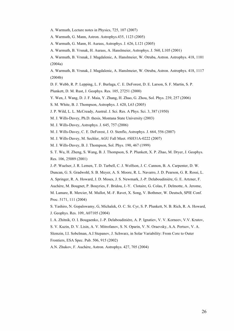
26
A. Warmuth, Lecture notes in Physics, 725, 107 (2007)
A. Warmuth, G. Mann, Astron. Astrophys.435, 1123 (2005)
A. Warmuth, G. Mann, H. Aurass, Astrophys. J. 626, L121 (2005)
A. Warmuth, B. Vrsnak, H. Aurass, A. Hanslmeier, Astrophys. J. 560, L105 (2001)
A. Warmuth, B. Vrsnak, J. Magdalenic, A. Hanslmeier, W. Otruba, Astron. Astrophys. 418, 1101
(2004a)
A. Warmuth, B. Vrsnak, J. Magdalenic, A. Hanslmeier, W. Otruba, Astron. Astrophys. 418, 1117
(2004b)
D. F. Webb, R. P. Lepping, L. F. Burlaga, C. E. DeForest, D. E. Larson, S. F. Martin, S. P.
Plunkett, D. M. Rust, J. Geophys. Res. 105, 27251 (2000)
Y. Wen, J. Wang, D. J. F. Maia, Y. Zhang, H. Zhao, G. Zhou, Sol. Phys. 239, 257 (2006)
S. M. White, B. J. Thompson, Astrophys. J. 620, L63 (2005)
J. P. Wild, L. L. McCready, Austral. J. Sci. Res. A Phys. Sci. 3, 387 (1950)
M. J. Wills-Davey, Ph.D. thesis, Montana State University (2003)
M. J. Wills-Davey, Astrophys. J. 645, 757 (2006)
M. J. Wills-Davey, C. E. DeForest, J. O. Stenflo, Astrophys. J. 664, 556 (2007)
M. J. Wills-Davey, M. Sechler, AGU Fall Meet. #SH31A-0222 (2007)
M. J. Wills-Davey, B. J. Thompson, Sol. Phys. 190, 467 (1999)
S. T. Wu, H. Zheng, S. Wang, B. J. Thompson, S. P. Plunkett, X. P. Zhao, M. Dryer, J. Geophys.
Res. 106, 25089 (2001)
J.-P. Wuelser, J. R. Lemen, T. D. Tarbell, C. J. Wolfson, J. C. Cannon, B. A. Carpenter, D. W.
Duncan, G. S. Gradwohl, S. B. Meyer, A. S. Moore, R. L. Navarro, J. D. Pearson, G. R. Rossi, L.
A. Springer, R. A. Howard, J. D. Moses, J. S. Newmark, J.-P. Delaboudiniére, G. E. Artzner, F.
Auchère, M. Bougnet, P. Bouyries, F. Bridou, J.-Y. Clotaire, G. Colas, F. Delmotte, A. Jerome,
M. Lamare, R. Mercier, M. Mullot, M.-F. Ravet, X. Song, V. Bothmer, W. Deutsch, SPIE Conf.
Proc. 5171, 111 (2004)
S. Yashiro, N. Gopalswamy, G, Michalek, O. C. St. Cyr, S. P. Plunkett, N. B. Rich, R. A. Howard,
J. Geophys. Res. 109, A07105 (2004)
I. A. Zhitnik, O. I. Bougaenko, J.-P. Delaboudiniére, A. P. Ignatiev, V. V. Korneev, V.V. Krutov,
S. V. Kuzin, D. V. Lisin, A. V. Mitrofanov, S. N. Oparin, V. N. Oraevsky, A.A. Pertsov, V. A.
Slemzin, I.I. Sobelman, A.I Stepanov, J. Schwarz, in Solar Variability: From Core to Outer
Frontiers, ESA Spec. Pub. 506, 915 (2002)
A.N. Zhukov, F. Auchère, Astron. Astrophys. 427, 705 (2004)
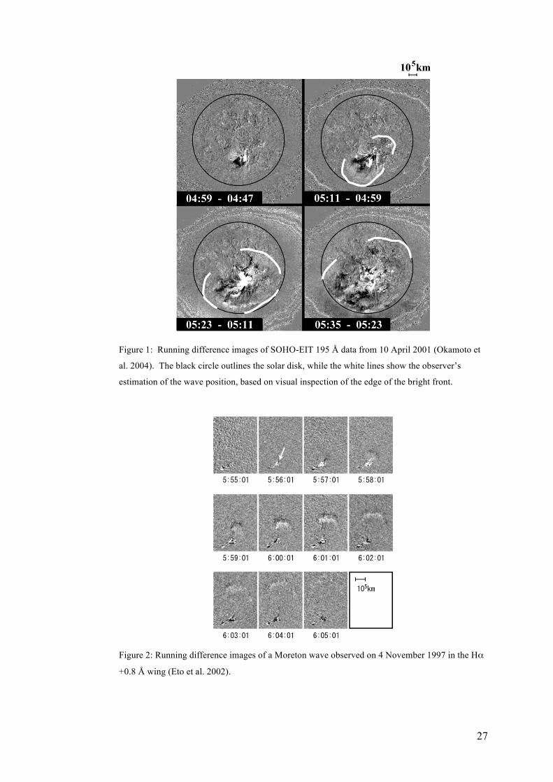
27
Figure 1: Running difference images of SOHO-EIT 195 Å data from 10 April 2001 (Okamoto et
al. 2004). The black circle outlines the solar disk, while the white lines show the observer’s
estimation of the wave position, based on visual inspection of the edge of the bright front.
Figure 2: Running difference images of a Moreton wave observed on 4 November 1997 in the Hα
+0.8 Å wing (Eto et al. 2002).
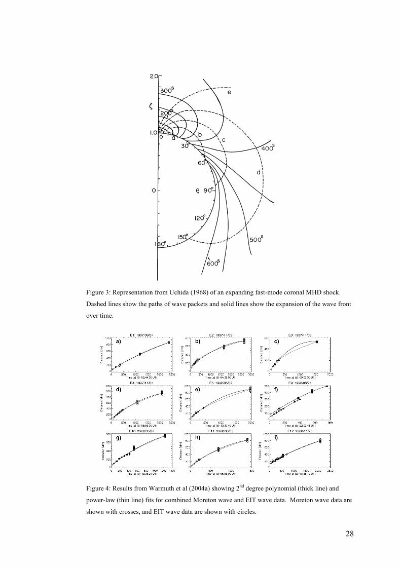
28
Figure 3: Representation from Uchida (1968) of an expanding fast-mode coronal MHD shock.
Dashed lines show the paths of wave packets and solid lines show the expansion of the wave front
over time.
Figure 4: Results from Warmuth et al (2004a) showing 2nd degree polynomial (thick line) and
power-law (thin line) fits for combined Moreton wave and EIT wave data. Moreton wave data are
shown with crosses, and EIT wave data are shown with circles.

29
Figure 5: Distribution of average EIT wave speeds with respect to “quality rating,” a subjective
quantity corresponding to the observer's confidence in the measurement (Wills-Davey et al. 2007).
This sample of 160 events shows a weak positive correlation. Note the substantial velocity spread.
Figure 6: (A) Successive base difference images showing the diffuse EIT wave event of 7 April
1997 (Attrill et al. 2007a). The bright fronts are overlaid with concentric black ellipses; the white
crosses mark the axes of the ellipses. (B) Quantitative measurements taken from the black ellipses
in (A), showing the mean intensity around the ellipses as a function of the deprojected azimuthal
angle. The vertical lines mark the weighted mean for each peak. The upper panel shows the
rotational shift of the mean-weighted peaks. The lower panel shows the weighted mean of the
later peaks phase-shifted to match those of the earlier peaks.
A) B)
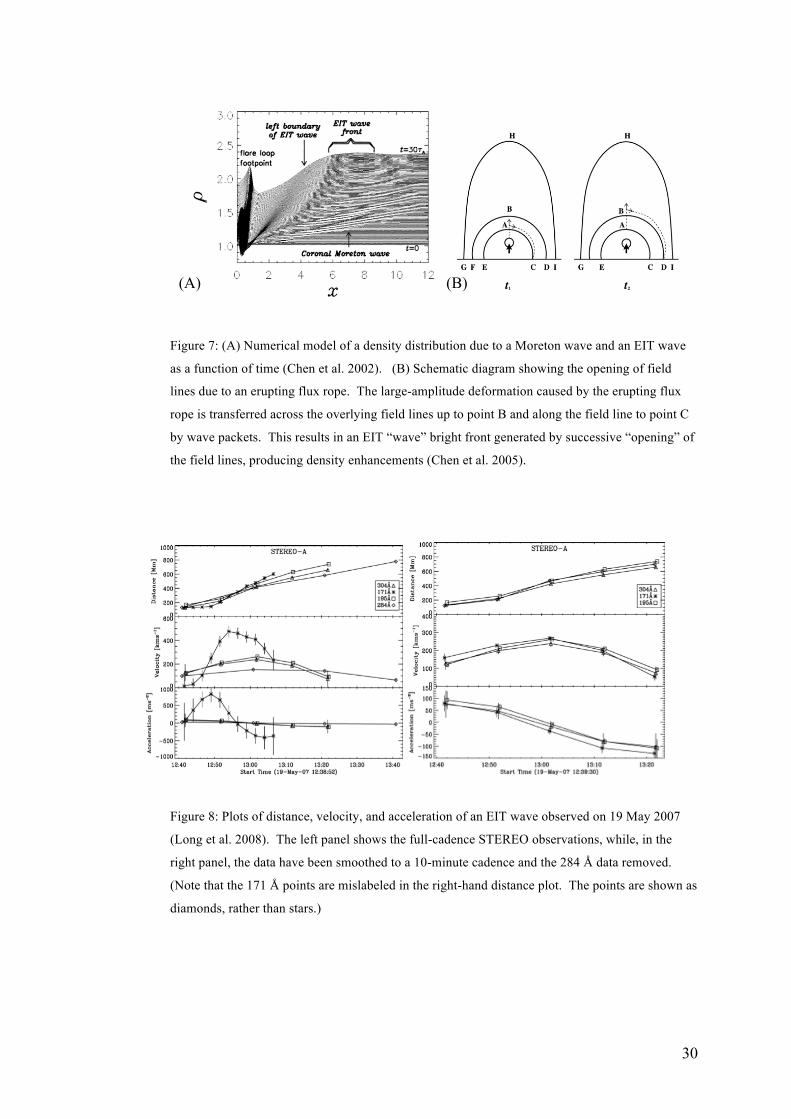
30
Figure 7: (A) Numerical model of a density distribution due to a Moreton wave and an EIT wave
as a function of time (Chen et al. 2002). (B) Schematic diagram showing the opening of field
lines due to an erupting flux rope. The large-amplitude deformation caused by the erupting flux
rope is transferred across the overlying field lines up to point B and along the field line to point C
by wave packets. This results in an EIT “wave” bright front generated by successive “opening” of
the field lines, producing density enhancements (Chen et al. 2005).
Figure 8: Plots of distance, velocity, and acceleration of an EIT wave observed on 19 May 2007
(Long et al. 2008). The left panel shows the full-cadence STEREO observations, while, in the
right panel, the data have been smoothed to a 10-minute cadence and the 284 Å data removed.
(Note that the 171 Å points are mislabeled in the right-hand distance plot. The points are shown as
diamonds, rather than stars.)
(A) (B)
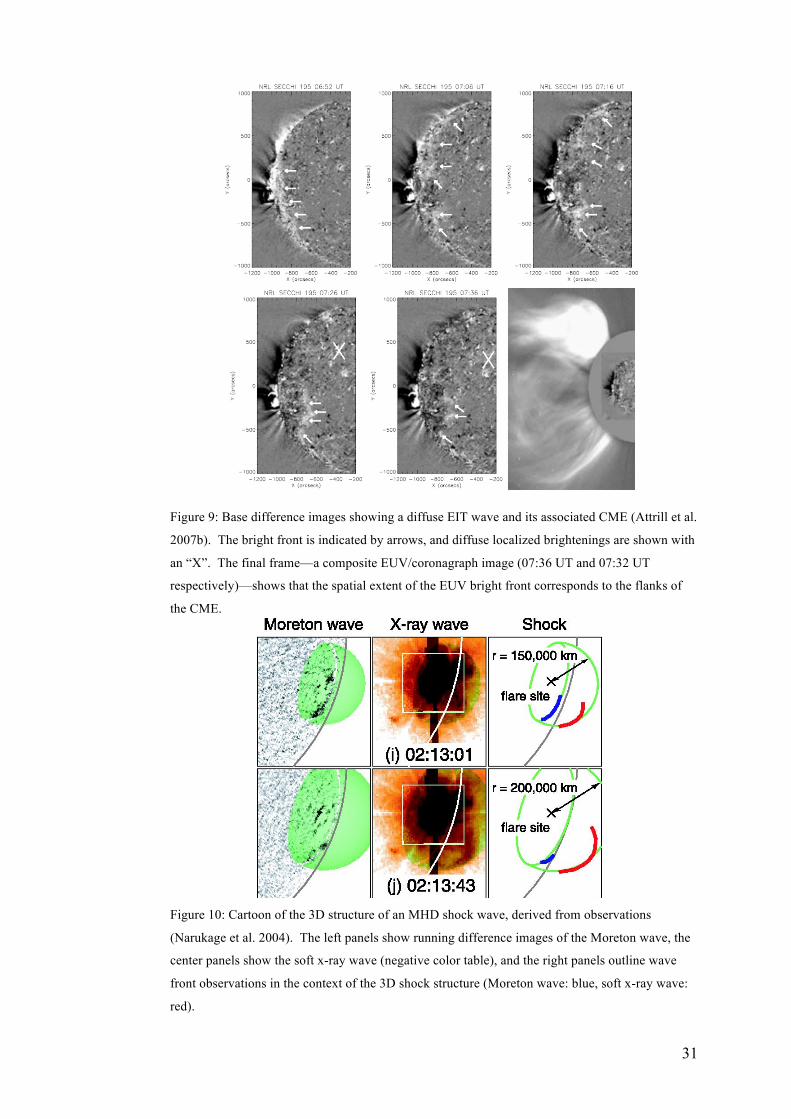
31
Figure 9: Base difference images showing a diffuse EIT wave and its associated CME (Attrill et al.
2007b). The bright front is indicated by arrows, and diffuse localized brightenings are shown with
an “X”. The final frame—a composite EUV/coronagraph image (07:36 UT and 07:32 UT
respectively)—shows that the spatial extent of the EUV bright front corresponds to the flanks of
the CME.
Figure 10: Cartoon of the 3D structure of an MHD shock wave, derived from observations
(Narukage et al. 2004). The left panels show running difference images of the Moreton wave, the
center panels show the soft x-ray wave (negative color table), and the right panels outline wave
front observations in the context of the 3D shock structure (Moreton wave: blue, soft x-ray wave:
red).
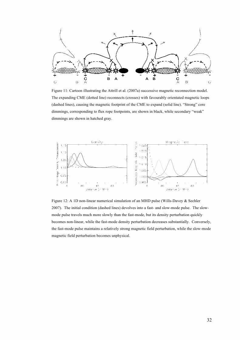
32
Figure 11: Cartoon illustrating the Attrill et al. (2007a) successive magnetic reconnection model.
The expanding CME (dotted line) reconnects (crosses) with favourably orientated magnetic loops
(dashed lines), causing the magnetic footprint of the CME to expand (solid line). “Strong” core
dimmings, corresponding to flux rope footpoints, are shown in black, while secondary “weak”
dimmings are shown in hatched gray.
Figure 12: A 1D non-linear numerical simulation of an MHD pulse (Wills-Davey & Sechler
2007). The initial condition (dashed lines) devolves into a fast- and slow-mode pulse. The slow-
mode pulse travels much more slowly than the fast-mode, but its density perturbation quickly
becomes non-linear, while the fast-mode density perturbation decreases substantially. Conversely,
the fast-mode pulse maintains a relatively strong magnetic field perturbation, while the slow-mode
magnetic field perturbation becomes unphysical.


