Proceedings of the 15th IBPSA ConferenceSan Francisco, CA, USA, Aug. 7-9, 2017
1121https://doi.org/10.26868/25222708.2017.293
Energy Performance of Membrane Energy Recovery Ventilation in Combination with an
Exhaust Air Heat Pump
Fabian Ochs1, Martin Hauer1, Michele Bianchi Janetti1, Siegele Dietmar1
1University of Innsbruck, Unit for Energy Efficient Buildings, Innsbruck
Abstract
Since the first discussion on energy recovery ventilation
(ERV) in the literature some years ago, several papers
were published about thermal comfort, performance and
ERV modelling. However, a combination of membrane
ERV and exhaust air heat pump (such as in a Passive
House compact unit for ventilation, heating and DHW
preparation) was not discussed in any of the previous
studies. In an exhaust air heat pump, the exhaust air is the
source of the heat pump and its performance is directly
connected to the effectiveness of the ERV. The
effectiveness of the ERV depends on the operation and
boundary conditions (in particular the average relative
humidity and the volume flow). Both are strongly coupled
to the building and its use and operation. By means of
simulation the complex dependencies are investigated.
Simulation models for ERV are developed and compared
against experimental data from the literature. For equal
indoor air relative humidity, the air exchange rate can be
significantly increased with ERV compared to a heat
recovery ventilation (HRV). This will lead to a further
improvement of the indoor air quality and to a significant
better of the performance of the heat pump and an increase
of the heating capacity.
Introduction
Air-to-air membrane energy recovery ventilation (ERV)
is increasingly discussed as a solution in residential
buildings for reducing the energy consumed for heating
and cooling as well as for improving the indoor air quality
by dehumidifying or humidifying the ventilation air.
Membrane based total energy (or so-called enthalpy)
exchangers allow for simultaneous heat and moisture
transfer through a selectively permeable membrane. In
cold climates, the problem of dry air in winter may be
reduced and frosting may be prevented or at least reduced
when the exhaust air is sufficiently dry after the moisture
recovery. However, there is the disadvantage of
significantly higher investment costs for a membrane
ERV compared to a heat recvovery ventilation (HRV). In
addition, there is an increased risk of mould growth in
transition times (spring, autumn) or when applied in new
buildings with high construction moisture content.
In combination with exhaust air heat pumps, ERV seems
to be a very promising solution. Usually the specific
heating power is limited to approx. 10 W/m² in such
heating systems as the specific heating power is coupled
to the hygienic flow rate (assuming 20 to 30 m³/h/P and a
average occupation density of 30 m²/P). Excessive flow
rates should be avoided in order to prevent too dry air, in
particular in cold climates. Higher volume flows can be
realized with ERV compared to HRV without violating
the lower limit for the indoor relative humidity (rH).
Review of ERV
Energy Recovery Ventilation ERV was proposed by some
authors e.g. by Schnieders et al. (2008) or Zhang et al.
(2010) already several years ago and since then quite
some work was done, as can be seen in the review papers
that were recently published, see e.g. Alonso et al. (2015).
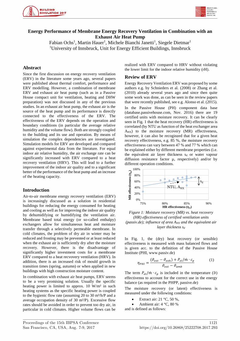
In the Passive House (PH) component data base
(database.passivehouse.com, Nov. 2016) there are 19
certified units with moisture recovery. It can be clearly
seen in Fig. 1 that the heat recovery (HR) effectiveness is
correlated (by NTU as function of the heat exchanger area
AHX) to the moisture recovery (MR) effectiveness,
however, it can also be recoginzed that for a given heat
recovery effectiveness, e.g. 85 %, the moisture recovery
effectiveness can vary between 47 % and 77 % which can
be explained either by different membrane properties (i.e.
the equivalent air layer thickness sd or water vapour
diffusion resistance factor µ, respectively) and/or by
different operation conditions.
Figure 1: Moisture recovery (MR) vs. heat recovery
(HR) effectiveness of certified ventilation units
(passiv.de); influence of area AHX and the equivalent air
layer thickness sd
In Fig. 1, the (dry) heat recovery (or sensible)
effectiveness is measured with mass balanced flows and
is given acc. to the definition of the Passive House
Institute (PHI, www.passiv.de)
𝜂𝑃𝐻𝐼 =(𝜗𝑒𝑥𝑡 − 𝜗𝑒𝑥ℎ) + 𝑃𝑒𝑙/�̇� ∙ 𝑐𝑝
𝜗𝑒𝑥𝑡 − 𝜗𝑎𝑚𝑏
(1)
The term 𝑃𝑒𝑙/�̇� ∙ 𝑐𝑝 is included in the temperature ()
effectivenss to account for the correct use in the energy
balance (as required in the PHPP, passive.de)
The moisture recovery (or latent) effectiveness is
measured under the following conditions:
Extract air: 21 °C, 50 %,
Ambient air: 4 °C, 80 %
and is defined as follows:
0%
20%
40%
60%
80%
100%
75% 80% 85% 90%
MR
eff
ecti
ven
ess
(hw)
HR effectiveness (hT)
NTU, AHX
sd

Proceedings of the 15th IBPSA ConferenceSan Francisco, CA, USA, Aug. 7-9, 2017
1122
𝜂𝜔 =𝜔𝑒𝑥𝑡 − 𝜔𝑒𝑥ℎ
𝜔𝑒𝑥𝑡 − 𝜔𝑎𝑚𝑏
(2)
with the humidity ratio w. For the energy balance
calculation within the PHPP the declared heat recovery
effectiveness (PHI definition) is increased according to
𝜂𝑃𝐻𝐼,𝑑𝑒𝑐𝑙𝑎𝑟𝑒𝑑 = 𝜂𝑃𝐻𝐼 + 𝑚𝑖𝑛(0.048 ; 𝜂𝜔 ∙ 0.08) (3)
in order to account for the influence on the moisture
balance (e.g. moisture buffer of walls) and the enhanced
enthalpy transfer in case of ERV compared to HRV.
Flow rates of mechanical ventilation with heat recovery
(MVHR) units reported on (www.passiv.de, < 600 m³/h)
vary from 60 m³/h to 460 m³/h with 160 m³/h in average,
see Table 1. If the same MVHR uses a membrane
moisture recovery heat exchanger (ERV) instead of a heat
recovery exchanger (HRV) with the same dimensions (i.e.
same volume), the declared heat recovery effectiveness is
reduced by about 2 to 9 %-points depending on the
volume flow. Correspondingly, applying eq. (3) the
measured HR is reduced by about 7 to 14 %-points.
Table 1: Heat recovery (HR) effectiveness hPHI,declared of
HRV and heat and moisture recovery (MR) effectiveness
of ERV of different MVHRs (�̇� < 600 m³/h) according to
PHI (passive.de)
No.
�̇� min
[m³/h]
�̇� max
[m³/h]
HR [%]
(HRV)
HR [%] MR [%]
(ERV)
1 70 270 90 86 73
2 70 345 88 83 71
3 70 460 87 80 68
4 85 290 86 82 67
5 73 109 89 85 64
6 73 115 89 85 64
7 80 111 86 83 71
8 121 231 93 84 73
9 65 200 87 85 77
10 110 280 83 81 63
11 80 111 86 83 71
12 116 368 90 85 71
13 116 246 92 87 74
Building Energy and Moisture Balance
Moisture Balance
Recommended ventilation rates of 20 to 30 m³/h/P are a
compromise between good indoor air quality (IAQ),
acceptable ventilation losses and sufficient relative
humidity, which should not fall below 30 %. Thermal
comfort can be guaranteed for a wide range of volume
flows if a heat recovery ventilation is used. Without
MVHR, excessive air exchange rates have to be avoided
in order to prevent from cold air down draught.
For a standard occupation density of 30 m²/P, a room
height of 2.7 m and a ventilation rate of 30 m³/h/P, an
infiltration rate corresponding to a n50-value of 0.6 1/h and
a moisture source of �̇�𝑣 = 100 g/P/h, the corresponding
indoor air relative humidity can be easily calculated acc.
to the steady state moisture balance:
�̇�𝑣,𝑖𝑛 − �̇�𝑣,𝑜𝑢𝑡 + �̇�𝑣 = 0 (4)
with the inlet vapour mass flow
�̇�𝑣,𝑖𝑛 = �̇�𝑎,𝑖𝑛𝑓 ∙ 𝜔𝑎𝑚𝑏+�̇�𝑎,𝑣𝑒𝑛𝑡 ∙ 𝜔𝑠𝑢𝑝 (5)
and outlet vapour mass flow
�̇�𝑣,𝑜𝑢𝑡 = (�̇�𝑎,𝑖𝑛𝑓 + �̇�𝑎,𝑣𝑒𝑛𝑡) ∙ 𝜔𝑒𝑥𝑡 (6)
For an ambient temperature of 𝜗𝑎𝑚𝑏 = 0 °𝐶 with a
relative humidity of 𝜑𝑎𝑚𝑏 = 80 % and an extract air
temperature of 𝜗𝑒𝑥𝑡 = 22 °𝐶 the corresponding indoor air
relative humidity is 33 % assuming an heat recovery
effectiveness of hT = 82 %. The supply air temperature is
then 19 °C with a rel. humidity of 23 %.
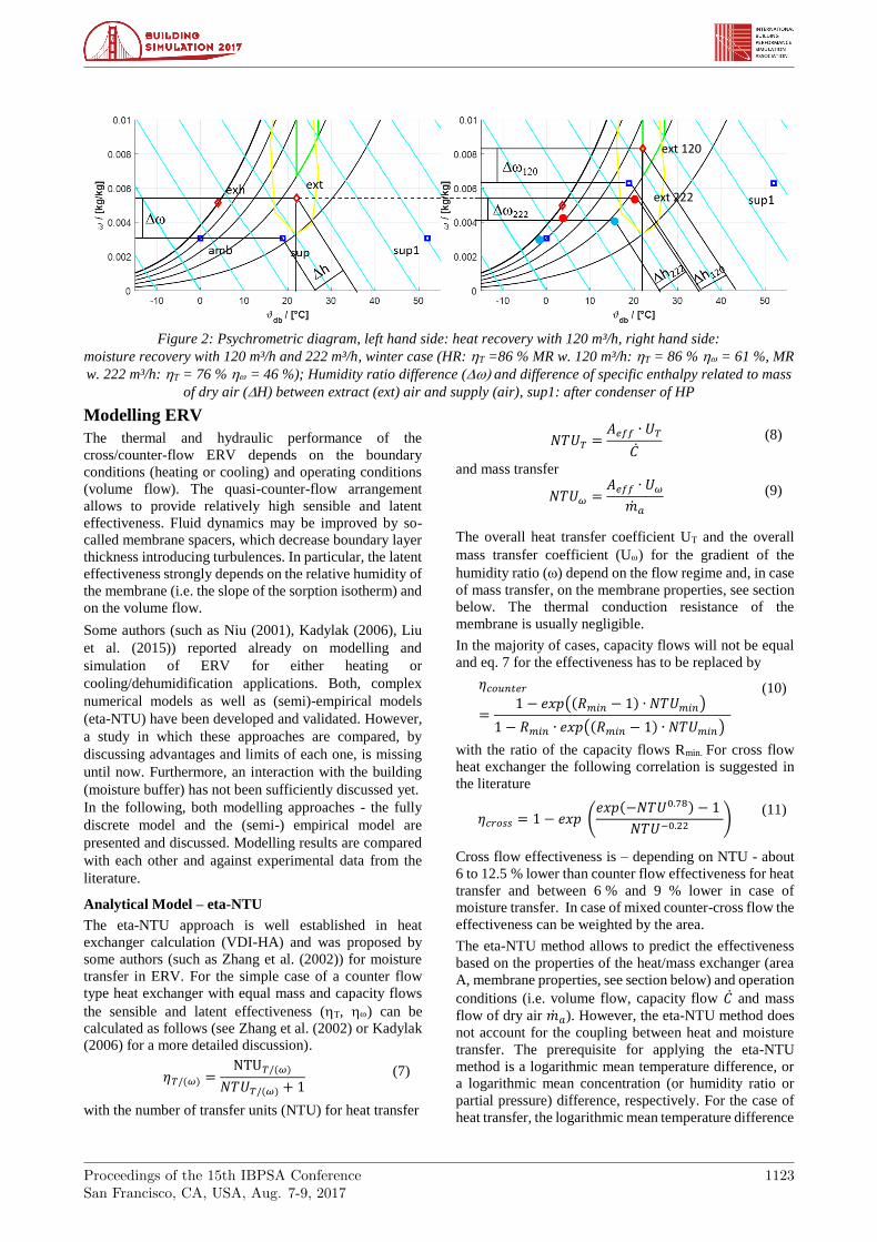
Moisture equivalent volume flow
Using instead an ERV with a moisture effectiveness of
64 % (for 120 m³/h in this example) for the same
conditions an indoor relative humidity of 49.7 % could be
obtained, see psychrometric diagram, Fig. 2. The
ventilation losses (enthalpy difference between extract air
and supply air) decrease from 394 W to 356 W. Hence,
assuming the same flow rate for HRV and ERV, the
indoor (i.e extract) air relative humidity is significantly
higher and it is in the comfort zone with ERV. The IAQ
would be better with respect to the relative humidity and
equal with respect to CO2- and/or TVOC-concentration,
respectively. (Remark: in this simplified moisture
balance, buffer storage effects and the influence of rH on
moisture sources are disregarded).
It is difficult to monetarize the better air quality and
thermal comfort (i.e. the higher relative humidity).
However, instead, we could assume to increase the flow
rate such that we obtain equal relative humidity compared
to the case without moisture recovery. This “moisture
equivalent volume flow” cannot be easily determined as
the temperature and moisture effectivenesses change with
the volume flow but it has to be determined by means of
inverse simulation. To obtain the same indoor air
humidity as in case of heat recovery the volume flow can
be increased from 120 m³/h to 222 m³/h. For the same heat
exchanger area, the temperature effectiveness decreases
by 12 %-points and the moisture transfer effectiveness by
16 %-points (see next section for a detailed description of
the model). Hence, the supply air decreases to 16.8 °C
with a relative humidity of 34.6 %, see (Fig. 2, right hand
side). The ventilation losses increase because of the
higher flow rate to 676 W. The additional ventilation
losses have to be covered by the heat pump, which will,
however, run with better COP.
The IAQ can be improved and due to the higher air flow
rate, more energy can be transported with the air (see state
sup1, after the condenser) and the efficiency of the
exhaust air heat pump can be increased if the same heating
power is assumed. There is an additional advantage of
significantly reducing the pre-heating energy demand
(frost-protection) which has to be considered, see also
section “ERV and Exhaust Air Heat Pump”, below.
Proceedings of the 15th IBPSA ConferenceSan Francisco, CA, USA, Aug. 7-9, 2017
1123
Figure 2: Psychrometric diagram, left hand side: heat recovery with 120 m³/h, right hand side:
moisture recovery with 120 m³/h and 222 m³/h, winter case (HR: hT =86 % MR w. 120 m³/h: hT = 86 % hw = 61 %, MR
w. 222 m³/h: hT = 76 % hw = 46 %); Humidity ratio difference (w and difference of specific enthalpy related to mass
of dry air (H) between extract (ext) air and supply (air), sup1: after condenser of HP
Modelling ERV
The thermal and hydraulic performance of the
cross/counter-flow ERV depends on the boundary
conditions (heating or cooling) and operating conditions
(volume flow). The quasi-counter-flow arrangement
allows to provide relatively high sensible and latent
effectiveness. Fluid dynamics may be improved by so-
called membrane spacers, which decrease boundary layer
thickness introducing turbulences. In particular, the latent
effectiveness strongly depends on the relative humidity of
the membrane (i.e. the slope of the sorption isotherm) and
on the volume flow.
Some authors (such as Niu (2001), Kadylak (2006), Liu
et al. (2015)) reported already on modelling and
simulation of ERV for either heating or
cooling/dehumidification applications. Both, complex
numerical models as well as (semi)-empirical models
(eta-NTU) have been developed and validated. However,
a study in which these approaches are compared, by
discussing advantages and limits of each one, is missing
until now. Furthermore, an interaction with the building
(moisture buffer) has not been sufficiently discussed yet.
In the following, both modelling approaches - the fully
discrete model and the (semi-) empirical model are
presented and discussed. Modelling results are compared
with each other and against experimental data from the
literature.
Analytical Model – eta-NTU
The eta-NTU approach is well established in heat
exchanger calculation (VDI-HA) and was proposed by
some authors (such as Zhang et al. (2002)) for moisture
transfer in ERV. For the simple case of a counter flow
type heat exchanger with equal mass and capacity flows
the sensible and latent effectiveness (hT, hw) can be
calculated as follows (see Zhang et al. (2002) or Kadylak
(2006) for a more detailed discussion).
𝜂𝑇/(𝜔) =NTU𝑇/(𝜔)
𝑁𝑇𝑈𝑇/(𝜔) + 1 (7)
with the number of transfer units (NTU) for heat transfer
𝑁𝑇𝑈𝑇 =𝐴𝑒𝑓𝑓 ∙ 𝑈𝑇
�̇� (8)
and mass transfer
𝑁𝑇𝑈𝜔 =𝐴𝑒𝑓𝑓 ∙ 𝑈𝜔
�̇�𝑎
(9)
The overall heat transfer coefficient UT and the overall
mass transfer coefficient (Uw) for the gradient of the
humidity ratio (w) depend on the flow regime and, in case
of mass transfer, on the membrane properties, see section
below. The thermal conduction resistance of the
membrane is usually negligible.
In the majority of cases, capacity flows will not be equal
and eq. 7 for the effectiveness has to be replaced by
𝜂𝑐𝑜𝑢𝑛𝑡𝑒𝑟
=1 − 𝑒𝑥𝑝((𝑅𝑚𝑖𝑛 − 1) ∙ 𝑁𝑇𝑈𝑚𝑖𝑛)
1 − 𝑅𝑚𝑖𝑛 ∙ 𝑒𝑥𝑝((𝑅𝑚𝑖𝑛 − 1) ∙ 𝑁𝑇𝑈𝑚𝑖𝑛)
(10)
with the ratio of the capacity flows Rmin. For cross flow
heat exchanger the following correlation is suggested in
the literature
𝜂𝑐𝑟𝑜𝑠𝑠 = 1 − 𝑒𝑥𝑝 (𝑒𝑥𝑝(−𝑁𝑇𝑈0.78) − 1
𝑁𝑇𝑈−0.22)
(11)
Cross flow effectiveness is – depending on NTU - about
6 to 12.5 % lower than counter flow effectiveness for heat
transfer and between 6 % and 9 % lower in case of
moisture transfer. In case of mixed counter-cross flow the
effectiveness can be weighted by the area.
The eta-NTU method allows to predict the effectiveness
based on the properties of the heat/mass exchanger (area
A, membrane properties, see section below) and operation
conditions (i.e. volume flow, capacity flow �̇� and mass
flow of dry air �̇�𝑎). However, the eta-NTU method does
not account for the coupling between heat and moisture
transfer. The prerequisite for applying the eta-NTU
method is a logarithmic mean temperature difference, or
a logarithmic mean concentration (or humidity ratio or
partial pressure) difference, respectively. For the case of
heat transfer, the logarithmic mean temperature difference
ext 120
ext 222
Proceedings of the 15th IBPSA ConferenceSan Francisco, CA, USA, Aug. 7-9, 2017
1124
applies only in case of dry conditions (no condensation,
no mass transfer). The eta-NTU does not allow predicting
the effectiveness depending on the boundary conditions
and on the mass transfer rate (as discussed in the
following sections).
Numerical Model
Numerical models for heat and mass transfer were
discussed already in the literature (see e.g. Zhang at al.
(1999), Jingchun et al. (2011), Yaïci et al. (2013)). For
cross flow ERVs, 2D models are required. 3D models are
usually not necessary as the conduction/diffusion in the
membrane in the direction of the flow can be disregarded
(see Zhang at al. (1999)).
For the simple case of a counter flow heat exchanger, the
following system of non-linear equations, which is
exemplarily given for stream 1 has to be solved.
Energy Balance
𝑐𝑝,𝑎 ∙ 𝜗1,𝑗 + 𝑚𝑖𝑛(𝜔𝑗 , 𝜔𝑗′) ∙ (𝑐𝑝,𝑣 ∙ 𝜗1,𝑗 + 𝛥ℎ𝑣)
= 𝑐𝑝,𝑎 ∙ 𝜗1,𝑗+1 + 𝑚𝑖𝑛(𝜔𝑗+1, 𝜔𝑗+1′ )
∙ (𝑐𝑝,𝑣 ∙ 𝜗1,𝑗+1 + 𝛥ℎ𝑣) +𝑈𝑇𝐴𝑒𝑓𝑓
�̇�𝑎,1
∙ (𝜗1,𝑗 − 𝜗2,𝑗)
(12)
Mass Balance
𝜔1,𝑗 = 𝜔1,𝑗+1 +𝑈𝑚,𝜔𝐴𝑒𝑓𝑓
�̇�𝑎,1
∙ 𝑑𝜔𝑣 (13)
In equations (12) and (13), is the temperature, w is the
humidity ratio, w' is the humidity ratio at saturation, cp is
the specific heat capacity at constant pressure for air (a)
and vapour (v), hv is the latent heat of vaporization and
ma,1 is the mass flow of dry air of stream 1. The overall
heat (UT) and moisture (Uw) transfer coefficients are
discussed in detail in the following sections.
The fsolve function in Matlab is used to solve the system
of N times 2 (streams) times 2 (mass and energy balance)
non-linear equations with N denoting the number of
segments. The boundary conditions are the temperature
and humidity ratio at both inlets (i.e. extract air and
ambient air). It was found that at least N > 150 nodes are
required to get sufficiently accurate results.
ERV – heat and mass transfer
Overall heat and mass transfer coefficient
The heat flux �̇� transferred in the heat exchanger is
porportional to the area A, the overall heat transfer
coefficient U and the logarithmic temperature difference
𝛥𝜗𝑙𝑜𝑔.
�̇� = 𝑈𝑇𝐴 ∙ Ψ ∙ 𝛥𝜗𝑙𝑜𝑔 (14)
Correspondingly, the mass transfer �̇�𝑣 can be calculated
with the overall mass transfer coefficient Um,p and the
logarithmic partial pressure difference.
�̇�𝑣 = 𝑈𝑚,𝑝𝐴 ∙ Ψm ∙ 𝛥𝑝𝑣,𝑙𝑜𝑔 (15)
Ψ is a correction factor, which is smaller than one, if heat
and mass transfer is different to the ideal case of counter
flow (e.g. in cross flow or in the case condensation
occurs).
The overall heat transfer coefficient is
𝑈𝑇 =1
1𝛼
+𝑑𝜆
+1𝛼
(16)
The conduction resistance of the membrane d/ is usually
negligible compared to the convective heat transfer
coefficient .
The overall mass transfer coefficient related to
concentration gradient Uc is a function of the mass
transfer coefficient and the diffusion resistance of the
membrane 𝑑𝑚𝑒𝑚/𝐷𝑚𝑒𝑚.
𝑈𝑐 =1
1𝛽
+𝑑𝑚𝑒𝑚
𝐷𝑚𝑒𝑚+
1𝛽
(17)
The overall mass transfer coefficient can also be defined
for the gradient of the humidity ratio (Uw) and for the
vapour pressure gradient (Up), while
𝑈𝜔 = 𝑈𝑐
𝑀𝑎 ∙ 𝑐𝑚
𝑥𝑎𝑚
(18)
and
𝑈𝑝 = 𝑈𝑐 ∙ 𝑅𝑣 ∙ 𝑇 (19)
In eqs. (18) and (19) Rv is the individual gas constant of
water, Ma the molar mass of air, cm the mean molar
concentration and xa,m the logarithmic mean molar
fraction of air, which depends on the humidity ratio w.
Heat and Mass Transfer Coefficient
The heat transfer coefficient can be calculated using
well known Nusselt (Nu) correlations with the thermal
conductivity () of the air and the hydraulic diameter
(dh).
𝛼 =𝑁𝑢 ∙ 𝜆
𝑑ℎ (20)
The flow through the heat exchanger can be assumed to
be laminar for all relevant volume flows because of the
narrow space in the channels. For heat transfer in
rectangular channels some authors suggest the following
Nu-correlation, which applies for fully developed flow
𝑁𝑢 = −7.4818 ∙ ar3 + 18.535 ∙ ar
2 − 15.663 ∙ ar + 8.235
(21)
with the aspect ratio ar.
𝑎𝑟 =ℎ𝑒𝑖𝑔ℎ𝑡
𝑤𝑖𝑑𝑡ℎ (22)
Other authors, e.g. Zhang et al. (1999) suggest Nu as a
function of Reynolds (Re) and Prandtl (Pr) number such
as:
𝑁𝑢
= 3.658 +0.085 ∙ (RePr
dh
L)
1 + 0.047 ∙ (RePrdh
L)
.67 ( ηb
ηs
)
.14
(23)
or
Proceedings of the 15th IBPSA ConferenceSan Francisco, CA, USA, Aug. 7-9, 2017
1125
𝑁𝑢 = 1.86 (Re ∙ Pr ∙ (dh
L))
.33
∙ ( ηb
ηs
)
.14
(24)
Nu depends on the hydraulic diameter dh and the length
of the channel L. The ratio of the dynamic viscosity of the
bulk b and the surface s ( ηb/ηs).14 can be disregarded
here, because of the low temperature differences. With
equations (23) and (24) the convective heat transfer
coefficient is in the range of 20 W/(m² K).
With equation (21) the convective heat transfer
coefficient takes values between 35.1 W/(m² K) for an
aspect ratio of 1 and 39.9 W/(m² K) for the actual aspect
ratio of 0.041 independent of the flow rate and assuming
fully developed flow. Gendebien at al. (2013) used
correlations given in Nellis et al. (2009), which use
corrections to consider the entrance region. For the
considered example (Zhong et al. (2014), see below), with
a cross section of the heat exchanger of
0.182 m x 0.462 m, a channel width of 2.5 mm, a
membrane thickness of 75 µm and 90 channels, the
convective heat transfer coefficient increases from
39.6 W/(m² K) to 41.2 W/(m² K) if the flow rate increases
from 100 to 200 m³/h.
Heat and mass transfer coefficients are correlated, as
shown by many authors. The well-known Lewis
correlation is
𝛽 =𝛼
𝜌𝑎𝑐𝑝,𝑎 ∙ 𝐿𝑒−2/3 (25)
The Lewis number
𝐿𝑒 =𝜆𝑎
𝜌𝑎𝑐𝑝,𝑎 ∙ 𝐷𝑣 (26)
is usually given with Le = 0.87 for these kind of
applications.
Membrane properties: diffusion through a
membrane
Vapor diffusion through a membrane can be described by
the first Fickian law which can be formulated as.
�̇�𝑣 =𝐷𝑣
𝑅𝑣 ∙ 𝑇 ∙ 𝑑𝑚𝑒𝑚 ∙ 𝜇∙ Δ𝑝𝑣 (27)
The equivalent air layer thickness sd is the product of the
membrane thickness dmem and the water vapour diffusion
resistance factor , which is a material property and
depends on the relative humidity as discussed in the
following.
𝑠𝑑 = 𝜇 ∙ 𝑑𝑚𝑒𝑚 (28)
In previous studies (e.g. Liu et al. 2015) the humidity
dependence of the vapour diffusion resistance factor µ
was mentioned, but usually it is disregarded.
The vapour diffusion resistance factor µ decreases with
the moisture content of the membrane u.
𝜇 = 𝐷𝑣
𝐷𝑚𝑒𝑚 ∙𝑑𝑢𝑑𝜙
∙𝑝𝑝𝑠
∙𝑀𝑣 ∙ 𝑐𝑚
𝑥𝑎,𝑚
(29)
Dv is the diffusion coefficient of moisture in air
𝐷𝑣 = 22.2𝐸 − 6 ∙ (1𝐸5
𝑝) ∙ (
𝑇𝑚
273.15)
1.81
(30)
and Dmem the diffusion coefficient of the membrane,
which has to be determined by experiments. The
saturation pressure ps can be approximated e.g.
𝑝𝑠 = 1.629𝐸11 ∙ 𝑒𝑥𝑝 (−5294
𝑇) (31)
p is the absolut pressure, Mv the molar mass, cm the mean
molar concentration and xa,m the logarithmic mean molar
fraction of air, which depends on the humidity ratio w
Niu et al. (2001)).
The moisture content of the membrane u is a function of
the relative humidity and can be described with the
sorption isotherm. A relative simple approach is given in
e.g. Alonso et al. (2015):
𝑢 =𝑢𝑚𝑎𝑥
1 − 𝐶 +𝐶𝜙
(32)
Then the derivative with respect to the rel. humidity is
𝑑𝑢
𝑑𝜙=
𝑐 ∙ 𝑢𝑚𝑎𝑥
(1 − 𝐶 +𝐶𝜙
)2
∙ 𝜙2
(33)
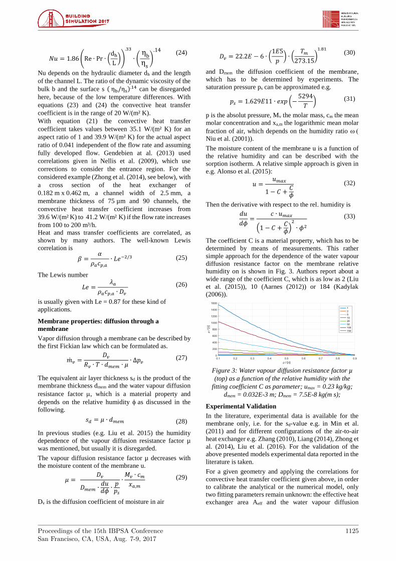
The coefficient C is a material property, which has to be
determined by means of measurements. This rather
simple approach for the dependence of the water vapour
diffusion resistance factor on the membrane relative
humidity on is shown in Fig. 3. Authors report about a
wide range of the coefficient C, which is as low as 2 (Liu
et al. (2015)), 10 (Aarnes (2012)) or 184 (Kadylak
(2006)).
Figure 3: Water vapour diffusion resistance factor µ
(top) as a function of the relative humidity with the
fitting coefficient C as parameter; umax = 0.23 kg/kg;
dmem = 0.032E-3 m; Dmem = 7.5E-8 kg(m s);
Experimental Validation
In the literature, experimental data is available for the
membrane only, i.e. for the sd-value e.g. in Min et al.
(2011) and for different configurations of the air-to-air
heat exchanger e.g. Zhang (2010), Liang (2014), Zhong et
al. (2014), Liu et al. (2016). For the validation of the
above presented models experimental data reported in the
literature is taken.
For a given geometry and applying the correlations for
convective heat transfer coefficient given above, in order
to calibrate the analytical or the numerical model, only
two fitting parameters remain unknown: the effective heat
exchanger area Aeff and the water vapour diffusion

Proceedings of the 15th IBPSA ConferenceSan Francisco, CA, USA, Aug. 7-9, 2017
1126
resistance factor µ. Contrariwise, if the flow regime is not
predictable with sufficient accuracy, the effective heat
transfer capability U.Aeff and the effective moisture
transfer capability Aeff/µ can be used as fitting parameters.
Three exemplary cases are considered: Liu et al. (2016)
present measured data of a relative small functional model
of a quasi-counter flow heat exchanger for winter
conditions (ext: 21 °C, 40 %). Zhong (2014) presents a
wide range of experimental results for a 0.182 m x
0.182 m x 0.462 m cross flow heat exchanger
configuration including different membranes and
different structures for summer conditions (ext: 27 °C,
50 % amb: 35 °C, 70 %). Two examples out of six are
considered here.
The sensible and latent effectiveness is shown as a
function of the volume flow in Fig. 4. Data from Liu et al.
(2016) is compared against the results of the eta-NTU
method and of the numerical model, described above.
With both methods, relative good agreement can be
obtained and the trends can be predicted well. The flow
rate influences both, the temperature effectiveness and the
moisture effectiveness hw, and has a major impact on the
latter. If the flow rate is doubled, e.g. from 30 m³/h to 60
m³/h the sensible effectivness decreases from 90 % to 85
%, while the latent effectivenss decreases from 72 % to
58 %.
The experimental results can be predicted with both, the
analytical (eta-NTU) and the numerical model rather well
in case of quasi-counter flow configuration. With the eta-
NTU method, better agreement between measured and
calculated data can be obtained assuming 40 % cross and
60 % counter flow with an effective area of Aeff = 10 m²
and a water vapour diffusion resistance of µ = 175 as
shown in Fig. 5.
The comparison of experimental data (from Zhong et al.
(2014)) with simulated data for the summer case is shown
in Fig. 6 and Fig. 7 for two cases with different plate type
membrane heat exchangers. Because of the cross flow
configuration, the 1D discrete model is not able to predict
the effectiveness very well: the decrease of the
effectiveness with the volume flow is overestimated. The
eta-NTU model delivers similar results for the latent
effectiveness, but it completely overestimates the sensible
effectiveness as the influence of latent on sensible heat
transfer is not considered (hT calculated with the eta-NTU
approach is not shown in Fig. 6 and 7). This effect is much
more pronounced in summer conditions, where the
temperature differences are generally lower (e.g. 35 °C-
27 °C = 8 K instead of 21 °C – 0 °C = 21 K).
The numerical model and the experimental data agree
quite well for the temperature effectivness in case of
membrane “C”, but there are relative large deviations in
case of type “E” in particular for low volume flows.
Effectivnesses shown in Fig. 4 and 5 are related to the
extract-exhaust air (hT1, hw1). In Fig. 6 and 7 the
effectiveness is the average between exhaust and extract
air (hT/w,1) and ambient and supply air (hT/w,2)
Figure 4: Sensible and latent effectiveness (marker, acc.
to Liu et al. (2016)); calculated (dashed line, eta-NTU)
and simulated (solid line) effectiveness as a function of
the volume flow; Aeff = 6 m², µ = 175;hT=
( ext- exh)/( ext- amb), hw=(w ext-w exh)/(w ext-wamb)
Figure 5: Sensible and latent effectiveness as a function
of the volume flow; measured (marker, acc. to Liu et al.
(2016)) and calculated with eta-NTU (dashed line,
counter-flow and dash-dotted line 40 cross flow);
Aeff = 10 m², µ = 250; hT/was in Fig. 4.
Figure 6: Sensible and latent measured (marker, acc. to
Zhong et al. (2014) “type E”) and simulated
effectiveness for a plate type heat exchanger in cross
flow configuration; (solid line, simulation), dashed and
dashed-dotted line eta-NTU; A = 22.5 m², µ = 125;
here: average effectiveness of both streams
hT/w=(hTw1+hTw2)/2
hT
hw h-NTU
40 % cross
h-NTU
counter
h-NTU
numeric
counter
cross
hT
hw
h-NTU numeric
Proceedings of the 15th IBPSA ConferenceSan Francisco, CA, USA, Aug. 7-9, 2017
1127
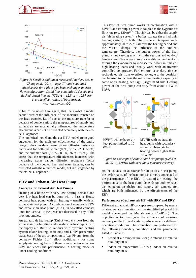
Figure 7: Sensible and latent measured (marker, acc. to
Zhong et al. (2014) “type C”) and simulated
effectiveness for a plate type heat exchanger in cross
flow configuration; (solid line, simulation), dashed and
dashed-dotted line eta-NTU; A = 12.5, µ = 125 here:
average effectiveness of both streams
hT/w=(hTw1+hTw2)/2
It has to be noted here again, that the eta-NTU model
cannot predict the influence of the moisture transfer on
the heat transfer, i.e. if due to the moisture transfer or
because of condensation, the temperatures of supply and
exhaust air are substantially influenced, the temperature
effectiveness can not be predicted accurately with the eta-
NTU approach.
The numerical model and the eta-NTU model are in good
agreement for the moisture effectiveness of the entire
range of the considered water vapour diffusion resistance
factor and for both, the winter (0 °C, 80 %, 22 °C 50 %)
and the summer case (35 °C, 80 %, 26 °C 50 %). The
effect that the temperature effectiveness increases with
increasing water vapour diffusion resistance factor
because of the coupled heat and mass transfer, can be
predicted with the numerical model, but is disregarded by
the eta-NTU approach.
ERV and Exhaust Air Heat Pump
Concepts for Exhaust Air Heat Pumps
Heating of a house with very low heating demand and
very low heat load can be done with a Passive House
compact heat pump with air heating – usually with an
exhaust air heat pump. A combination of membrane ERV
and exhaust air heat pump (as e.g. in so-called compact
units for Passive Houses) was not discussed in any of the
previous studies.
An exhaust air heat pump (EAHP) extracts heat from the
exhaust air of a building and transfers the heat typically to
the supply air. But also variants with hydronic heating
system (floor heating, radiators) and DHW preparation
exist. State of the art compact units (e.g. PKom4 from the
company Pichler Luft) allow additionally for some
supply-air cooling, but still there is no experience on how
ERV influences the performance in heating mode or
under cooling conditions.
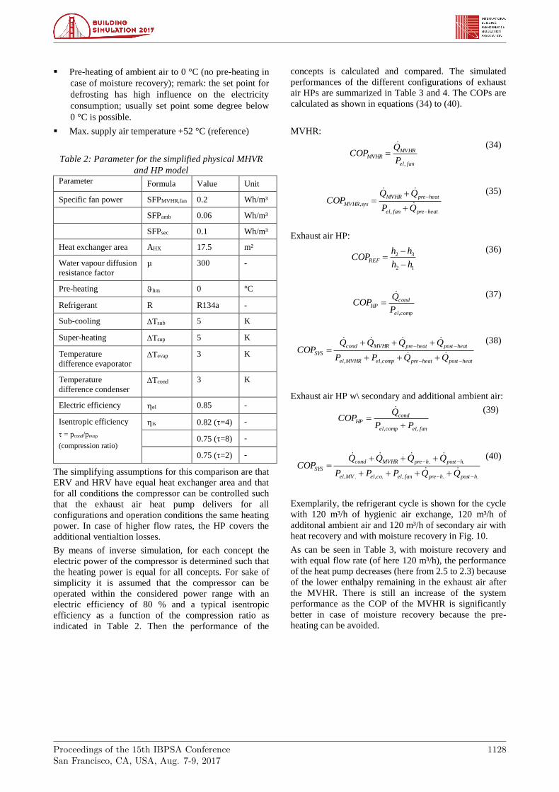
This type of heat pump works in combination with a
MVHR and its output power is coupled to the hygienic air
flow rate (e.g. 120 m³/h). The sink can be either the supply
air (air heating system), a buffer storage (in a hydronic
heating system) or both. The inside air temperature is
approximately 20 to 22 °C all over the heating period and
the MVHR damps the influence of the ambient
temperature. Therefore, the output power of the heat
pump is not varying much with the seasons and outdoor
temperature. Newer versions suck additional ambient air
through the evaporator to increase the power in times of
high heating loads and usually work with an inverter
controlled compressor. Furthermore, secondary air (i.e.
recirculated air from overflow zones, e.g. the corridor)
can be used to increase the maximum heating capacity in
caase of air heating, see Fig. 9, right hand side. Heating
power of the heat pump can vary from about 1 kW to
6 kW.
MVHR with exhaust air
heat pump limited to 10
W/m²
MVHR with exhaust air
heat pump with secondary
air and ambient air for
heating power higher than
10 W/m²
Figure 9: Concepts of exhaust air heat pumps (Ochs et
al. 2017), MVHR with or without moisture recovery
As the exhaust air as source for an air-to-air heat pump,
the performance of the heat pump is directly connected to
the performance of the ERV. In case of air heating, the
performance of the heat pump depends on both, exhaust
air temperature/enthalpy and supply air temperature,
which are both influenced by the effectiveness of the
ERV.
Performance of exhaust air HP with HRV and ERV
Different exhaust air HP concepts are compared by means
of steady-state simulation with a simplified physical HP
model (developed in Matlab using CoolProp). The
objective is to investigate the influence of moisture
recovery on the HP and system performance for different
operation conditions. The simulations are performed for
the following boundary conditions and the parameters
listed in Table 2:
Ambient air temperature -8°C; Ambient air relative
humidity 80 %
Indoor air temperature +22 °C; Indoor air relative
humidity 30 %
ambient exhaust
extract supply
h-NTU
numeric
counter
cross
ambient exhaust
extract supply
secondary
Proceedings of the 15th IBPSA ConferenceSan Francisco, CA, USA, Aug. 7-9, 2017
1128
Pre-heating of ambient air to 0 °C (no pre-heating in
case of moisture recovery); remark: the set point for
defrosting has high influence on the electricity
consumption; usually set point some degree below
0 °C is possible.
Max. supply air temperature +52 °C (reference)
Table 2: Parameter for the simplified physical MHVR
and HP model Parameter Formula Value Unit
Specific fan power SFPMVHR,fan 0.2 Wh/m³
SFPamb 0.06 Wh/m³
SFPsec 0.1 Wh/m³
Heat exchanger area AHX 17.5 m²
Water vapour diffusion
resistance factor
µ 300 -
Pre-heating lim 0 °C
Refrigerant R R134a -
Sub-cooling Tsub 5 K
Super-heating Tsup 5 K
Temperature
difference evaporator Tevap 3 K
Temperature
difference condenser Tcond 3 K
Electric efficiency hel 0.85 -
Isentropic efficiency
= pcond/pevap
(compression ratio)
his 0.82 (=4) -
0.75 (=8) -
0.75 (=2) -
The simplifying assumptions for this comparison are that
ERV and HRV have equal heat exchanger area and that
for all conditions the compressor can be controlled such
that the exhaust air heat pump delivers for all
configurations and operation conditions the same heating
power. In case of higher flow rates, the HP covers the
additional ventialtion losses.
By means of inverse simulation, for each concept the
electric power of the compressor is determined such that
the heating power is equal for all concepts. For sake of
simplicity it is assumed that the compressor can be
operated within the considered power range with an
electric efficiency of 80 % and a typical isentropic
efficiency as a function of the compression ratio as
indicated in Table 2. Then the performance of the
concepts is calculated and compared. The simulated
performances of the different configurations of exhaust
air HPs are summarized in Table 3 and 4. The COPs are
calculated as shown in equations (34) to (40).
MVHR:
fanel
MVHRMVHR
P
QCOP
,
(34)
heatprefanel
heatpreMVHR
sysMVHRQP
QQCOP
,
, (35)
Exhaust air HP:
12
32
hh
hhCOPREF
(36)
compel
condHP
P
QCOP
,
(37)
heatpostheatprecompelMVHRel
heatpostheatpreMVHRcond
SYSQQPP
QQQQCOP
,,
(38)
Exhaust air HP w\ secondary and additional ambient air:
fanelcompel
condHP
PP
QCOP
,,
(39)
..,.,.,
..
hposthprefanelcoelMVel
hposthpreMVHRcond
SYSQQPPP
QQQQCOP
(40)
Exemplarily, the refrigerant cycle is shown for the cycle
with 120 m³/h of hygienic air exchange, 120 m³/h of
additonal ambient air and 120 m³/h of secondary air with
heat recovery and with moisture recovery in Fig. 10.
As can be seen in Table 3, with moisture recovery and
with equal flow rate (of here 120 m³/h), the performance
of the heat pump decreases (here from 2.5 to 2.3) because
of the lower enthalpy remaining in the exhaust air after
the MVHR. There is still an increase of the system
performance as the COP of the MVHR is significantly
better in case of moisture recovery because the pre-
heating can be avoided.

Proceedings of the 15th IBPSA ConferenceSan Francisco, CA, USA, Aug. 7-9, 2017
1129
Figure 10: Temperature-enthalpy diagram (R134a) for the case with heat recovery (left) and moisture recovery
(right) for 120 m3/h hygienic air exchange, 120 m3/h additional ambient air and 120 m³/h secondary air; sup0 after
MVHR, before condenser, sup1 after condenser, exh0 after MFHR before evaporator, exh1 after evaporator
As discussed in the previous sections, with moisture
recovery, the hygienic air exchange rate can be increased
without violating the lower recommended boundary of the
relative humidity (usually 30 %). The moisture equivalent
volume flow with moisture recovery is 222 m³/h
compared to 120 m³/h.
Table 3: Results for the exhaust air heat pump (see Fig.
2 left hand side) for heat recovery(HR) with a volume
flow of 120 m³/h and with moisture recovery (MR) with
120, 150 and 222 m³/h; �̇�MVHR heat flux transferred by
MHVR, �̇�pre-heat: heat flux for frost-protection, �̇�HP: Heat flux
delivered by HP (condenser), �̇�loss,comp: thermal losses of
compressor, �̇�𝑒𝑥𝑡 − �̇�𝑠𝑢𝑝: ventilation losses, COPref: COP of
refrigerant cycle (based on specific enthalpies)
Quantity Unit HR
120
MR
120
MR
150
MR
222
rHext [-] 0.30 0.55 0.44 0.30
sup [°C] 18.8 17.6 16.7 14.7
rHsup [-] 0.11 0.48 0.39 0.30
hT1 [-] 0.85 0.85 0.82 0.76
hw1 [-] 0.00 0.60 0.55 0.45
hT2 [-] 0.85 0.85 0.82 0.76
hw2 [-] 0.00 0.60 0.55 0.45
�̇�MVHR [W] 1359 1632 1790 2172
�̇�pre-heat [W] 352 0 0.0 0.0
�̇�ext-�̇�sup [W] 525 532 657.4 980.1
sup1 [°C] 52.0 50.7 45.5 38.2
�̇�HP [W] 1466 1472 1597 1920
�̇�loss,comp [W] 81 90 86.0 84.7
COPMVHR,sys [-] 2.9 34.0 29.8 24.5
COPref [-] 2.7 2.5 2.8 3.4
COPHP [-] 2.5 2.3 2.5 2.9
COPsys [-] 2.8 4.5 5.4 6.3
The COP of the exhaust air HP can be increased from 2.5
(HR), or 2.3 (MR) at 120 m³/h to 2.9 at 222 m³/h.
If instead additional ambient air is used as source and
secondary air is used additionally in the condenser, the
COP can be improved from 2.5 to 3.1 in case of heat
recovery and from 2.3 to 2.9 in case of moisture recovery.
The improvement is less pronounced in case of higher air
flow rates, but with 8.9 % still relevant.
The maximum possible heating power can be improved
with both measures, moisture recovery and secondary air,
as can be seen from the supply air 1 in Table 3 and 4
(remark: max. air temperature should not exceed 52 °C).
Table 4: Results for the exhaust air heat pump with
120 m³/h recirculation and 120 m³/h additional ambient
air (see Fig. 2, right hand side) and comparison with
results acc. to Table 3.
Quantity Unit HR
120
MR
120
MR
150
MR
222
sup1 [°C] 37.7 37.2 35.7 32.9
�̇�HP [W] 1466 1472 1597 1921
�̇�loss,comp [W] 61 65 67.1 73.8
COPMVHR,sys [-] 2.9 34.0 29.8 24.5
COPref [-] 3.6 3.4 3.6 3.9
COPHP [-] 3.1 2.9 3.0 3.2
COPsys [-] 3.2 6.2 6.4 6.8
Rel. COPHP [%] 24.6 29.6 20.3 8.9
Rel. COPsys [%] 13.9 38.7 20.2 8.9
Conclusion
Particularly in combination with an exhaust air heat
pump, giving a recommendation of whether or not to use
a membrane ERV is not easily possible because of the
complex relations. The effectiveness cannot be used as
single decisive indicator. Moisture recovery allows
increasing the volume flow without violating the
recommended lower limit for indoor humidity. With
higher volume flow, IAQ can be improved and the
Tevap = 5 K
sup1
sup0
exh0
exh1
sup1
sup0
exh0 exh1
Proceedings of the 15th IBPSA ConferenceSan Francisco, CA, USA, Aug. 7-9, 2017
1130
performance of an exhaust air heat pump can be enhanced.
The presented results represent one working point.
Detailed building and system simulation are required to
determine the economic feasibility of moisture recovery
depending on the operation and boundary conditions such
as climate and occupation (i.e. internal heat and moisture
gains) profile.
Both models, the eta-NTU and the numerical model,
predict the influence of the volume flow rather well for
the winter case. In summer, the eta-NTU approach
overestimates the temperature effectiveness by far, as the
coupling of the heat and moisture transfer mechanisms are
not accounted for. The numerical model has to be used
here instead. However, there is need for improvement
with respect to mixed cross/counter flow configurations
and with respect to the convective heat transfer coefficient
and the membrane properties. The dependence of the
average rel. humidity on the water vapour diffusion
resistance factor cannot be directly recognised from the
considered cases. The mass transfer potential of different
membranes taken from the literature, e.g. Kadylak (2006)
does not correspond to the ones identified by the inverse
simulation. Further experimental work is required and
will be doen with the newly developed test stand for ERV
and compact units: Within the Austrian FFG project
“SaLüH!” measurements of the effectiveness of ERVs
and the influence on the performance of the exhaust air
heat pump will be performed for different boundary
conditions in the near future.
Future work must also focus an air distribution with a
transient multi-zone approach including moisture buffer.
Acknowledgement
This work is part of the Austrian research project SaLüH!
Renovation of multi-family houses with small apartments,
low-cost technical solutions for ventilation, heating & hot
water (2015-18); Förderprogramm Stadt der Zukunft,
FFG, Project number: 850085.
References
Aarnes SM. Membrane based heat exchanger. (M.Sc.
Thesis in Product Design and Manufacturing,
Department of Energy and Process Engineering).
Norway: Norwegian University of Science and
Technology; 2012
Alonso, M. J., Peng Liu, Martin H. M. Gaoming G.,
Simonson C. (2015), Review of heat/energy recovery
exchangers for use in ZEBs in cold climate countries.
Building and Environment. vol. 84, 2015.
Gendebien S., Bertagnolio S., Lemort V. (2013),
Investigation on a ventilation heat recovery
exchanger: Modeling and experimental validation in
dry and partially wet conditions, Energy and
Buildings, Vol 2, p176-189, Elsevier, 2013.
Kadylak D. E. (2006), Effectiveness Method for Heat and
Mass Transfer in Membrane Humidifieres, 2006.
Liang Caihang, (2014), Research on a Refrigeration
Dehumidification System with Membrane-Based
Total Heat Recovery, Heat Transfer Engineering,
Taylor and Francis, 2014.
Liu P., Alonso M.J., Martin, H. (2015), Membrane
Energy Exchanger, Evaluation of a frost-free design
and its performance for ventilation in cold climates,
Proceedings of the 24th International Congress of
Refrigeration, 2015.
Liu P., Alonso M.J., Mathisen, HM Simonson C. (2016),
gPerformance of a quasi-counter-flow air-to-air
membrane energyexchanger in cold climates, Energy
and Buildings 119 (2016) 129–142.
Min Jingchun, Hu Teng, Song Yaozu (2011),
Experimental and numerical investigations of
moisture permeation through membranes, Journal of
Membrane Science, Volume 367, Issues 1–2, 1
February 2011, Pages 174–181.
Nellis G.F., Klein S.A., (2009) Heat Transfer, Cambridge
University Press, 2009, Section 5.2.4.
Niu J. L. , Zhang L. Z. (2001), “Membrane-based
enthalpy exchanger: material considerations and
clarification of moisture resistance,” Journal of
membrane science, vol. 189, pp. 179–191, 2001.
Ochs F., Pfluger R., Dermentzis G., Siegele D., (2017)
Energy Efficient Renovation with Decentral
Compact, Heat Pumps, 12th IEA Heat Pump
Conference 2017, Rotterdam.
Schnieders J., Pfluger R., Feist W. (2008), Energetische
Bewertung von Wohnungslüftungsgeräten mit
Feuchterückgewinnung. Passivhaus Institut,
Darmstadt, 2008.
Wahiba Yaïci, Mohamed Ghorab, Evgueniy Entchev
(2013), Numerical analysis of heat and energy
recovery ventilators performance based on CFD for
detailed design, Applied Thermal Engineering 51
(2013) 770e780.
Zhang, L.-Z. Jiang Y. (1999), Heat and mass transfer in a
membrane-based energy recovery ventilator, Journal
of Membrane Science, Volume 163, Issue 1, 1
October 1999, Pages 29–38.
Zhang L. Z., Niu J. L., (2002), Effectiveness correlations
for heat and moisture transfer processes in an
enthalpy exchanger with membrane cores, Journal of
Heat Transfer, vol. 124, pp. 922–929, October 2002.
Zhang, L.-Z. (2010), Heat and mass transfer in a quasi-
counter flow membrane-based total heat exchanger.
International Journal of Heat and Mass Transfer
53(23-24): 5478-5486.
Zhong Ting-Shu, Li Zhen-Xing, Zhang Li-Zhi (2014)
Investigation of Membrane-Based Total Heat
Exchangers with. Different Structures and Materials,
Journal of Membrane and Separation Technology,
2014, 3, 1-10.
CoolProp: http://www.coolprop.org/ (visited 2016)


