
ENVIRONMENTAL ENGINEERING
EVALUATION OF THERMALLY ENHANCED SOIL VAPOR EXTRACTION
USING ELECTRICAL RESISTANCE HEATING FOR CHLORINATED
SOLVENT REMEDIATION IN THE VADOSE ZONE
ASHLEY HENDRICKS
Thesis under the direction of Professor David S. Kosson
Soil vapor extraction (SVE) is the most popular technology for removing volatile
contaminants from the vadose zone. However, SVE is limited by the contaminant vapor
pressure, hydraulic conductivity and gas permeability of the vadose stratigraphy.
Concentration reductions greater than 90% are hard to achieve with traditional SVE.
Thermal enhancement is establishing itself as a viable method to increase the
applicability and effectiveness of SVE. Heating methods include steam injection,
radiowave, microwave, and electrical resistance. The appropriate method depends on site
geology, soil and contaminant parameters and the maximum temperature required.
Electrical resistance heating (ERH) is one promising enhancement method. ERH has
been demonstrated at more than 30 sites. However, little is known about the mechanisms
occurring during the heating process. Existing models are limited in scope, neglecting
important aspects of heat and mass transfer.
ii
The purpose of the research presented is to develop the basis for a general mass
transfer model to simulate the SVE process during remediation of chlorinated solvents
using thermally enhanced SVE in the vadose zone. A conceptual model detailing the
processes occurring during vapor extraction with soil heating by electrical resistance is
proposed. The conceptual model is then used to derive a set of governing equations for a
general multiphase multicomponent system with an applied heat flux. This approach
allows the model developed here to be extended to other thermal treatments.
Approved:
David S. Kosson, Ph.D.

EVALUATION OF THERMALLY ENHANCED SOIL VAPOR EXTRACTION
USING ELECTRICAL RESISTANCE HEATING FOR CHLORINATED
SOLVENT REMEDIATION IN THE VADOSE ZONE
By
Ashley Hendricks
Thesis
Submitted to the Faculty of the
Graduate School of Vanderbilt University
in partial fulfillment of the requirements
for the degree of
MASTER OF SCIENCE
in
Environmental Engineering
May, 2006
Nashville, Tennessee
Approved:
David S. Kosson, Ph.D. Florence Sanchez, Ph.D. Christine Switzer, Ph.D.
ii
ACKNOWLEDGEMENTS
This thesis was prepared with the support of the U.S. Department of Energy,
under Award No. DE-FG01-03EW15336 to the Institute for Responsible Management,
Consortium for Risk Evaluation with Stakeholder Participation II. However, any
opinions, findings, conclusions, or recommendations expressed herein are those of the
author and do not necessarily reflect the views of the DOE or of IRM/CRESP II.
I would especially like to thank Drs. Christine Switzer and David Kosson for their
time, insights and putting up with me for nearly two years. Thanks are also in order for
Nicole Comstock – bless anyone who tries to keep track of Dr. Kosson. Thank you also
to Karen Page and Whitney Crouch for your support during my tenure at Vanderbilt.
Getting through my time at Vanderbilt would not have been possible without my
two Amigos: Jennifer Miller (the soon to be Mrs. Williams) and Janey Smith. Long
lunches and general ruckus-making would not have been as much fun without them. I
must also thank the wonderful website gotradio.com for keeping me entertained and
undistracted by the outside world.
I must acknowledge my parents, dear sister, Gretchen, and best friend, Athena.
Without them nothing in life would be possible. I hope I have made you proud. Lucky,
Sam and Shadow thank you so much for all your assistance with homework and typing.
Your incessant distractions and wet noses keep me sane.

iii
TABLE OF CONTENTS
Page
ACKNOWLEDGEMENTS ............................................................................................. ii
LIST OF TABLES .............................................................................................................v
LIST OF FIGURES ......................................................................................................... vi
LIST OF ABBREVIATIONS ........................................................................................ vii
Chapter
I. INTRODUCTION.....................................................................................................1
1.1 Overview ........................................................................................................1 1.2 Thesis Goals and Objectives ........................................................................2 II. LITERATURE REVIEW ........................................................................................4
2.1 Overview of Heating Techniques and Applications...................................4
2.1.1 Steam and Hot Air Injection ...............................................................6 2.1.2 Radio and Microwave Frequency.......................................................8 2.1.3 Electrical Resistance.........................................................................11 2.1.4 Summary and Conclusions................................................................14 2.1.4.1 Generalized Costs ..............................................................14 2.1.4.2 Recommendations and Decisionmaking............................14 2.2 Previous Approaches and Modeling..........................................................17 III. MODEL DEVELOPMENT ...................................................................................22 3.1 Conceptual Model .......................................................................................22 3.2 Governing Equations ..................................................................................27 3.2.1 Mass ..................................................................................................29 3.2.2 Momentum.........................................................................................30

iv
3.2.3 Energy ...............................................................................................39 3.3 Methodology for Model Solution.....................................................................42 IV. SUMMARY AND CONCLUSIONS .....................................................................43 Appendix A. KNOWN RELATIONSHIPS.................................................................................45 B. GOVERNING EQUATIONS (SUMMARIZED) ................................................48 REFERENCES.................................................................................................................51

v
LIST OF TABLES
Table Page
3-1: Flow Areas and Volumes ..........................................................................................22
3-2: Phase-Component Possibilities .................................................................................25

vi
LIST OF FIGURES
Figures Page
2-1: Vapor Pressure and Temperature for Selected Compounds .......................................5
2-2: Steam Injection Schematic ..........................................................................................7
2-3: Radiofrequency Heating Schematic .............................................................................9 2-4: Electrical Resistance Heating System .......................................................................12 2-5: Electrical Resistance Heating Electrode Layout .......................................................13 2-6: Decision Tool for Selecting the Most Appropriate Heating Technique....................16 3-1: Representative Slice ..................................................................................................22 3-2: Porous Medium Control Volume ..............................................................................23 3-3: Conceptual Representation of the Phases and Their Interactions .............................24 3-4: Radial Flow within the Porous Medium....................................................................25 3-5: Temperature Profile...................................................................................................26 3-6: Moisture Content along the Radial Axis ...................................................................26 3-7: Pressure Profile..........................................................................................................27

vii
NOMENCLATURE
Symbol Units A Area [m2] α Phase (l, s, g) a Surface a of control volume β Component (TCE, water, soil, air) b Surface b of control volume CP Specific heat at constant pressure [J/kg-K] Cv Specific heat at constant volume [J/kg-K] c Surface c of control volume CS Control surface CV Control volume d Surface d of control volume e Surface e of control volume F Force [N] Fg Force due to gravity [N] Fv Viscous force [N] FP Force due to pressure [N] f Surface f of control volume g Acceleration of gravity [m/s2] g Gas phase hvap Heat of vaporization [J/kg] H Specific enthalpy [J/kg] H Total enthalpy [J/kg]
vapH Heat of vaporization [J/kg] k Thermal conductivity [W/m-K] l Liquid phase m Mass [kg] m Mass transfer rate [kg/m3-s] Mw Molecular weight [g/mol] n Number of moles [mol] n Normal vector η Porosity [-]

viii
Symbol Units o Initial θ Moisture content [-] θl,NAPL Liquid NAPL content [-] θl,water Liquid water content [-] θg,total Total gas content [-] θg,NAPL Gaseous NAPL content [-] θg,water Gaseous water content [-] θl,total Total liquid content [-] φ Space coordinate P Pressure [atm] Po Initial pressure [atm] ρ Density [kg/m3] q Heat flux [W/m2] Q Heat generation [W/m3] r Space coordinate rw Radius of SVE well [m] r∞ Temperature far from the heated area [K] Rn Radius of circular area (radius to electrode) [m] R Universal Gas Constant [J/mol-K] ref Reference state (i.e. temperature, pressure) S Saturation [-] s Solid phase sur outer surface of circular area t Time [s] T Temperature [K] To Ambient temperature (before heating) [K] Tref Reference temperature [K]
Tsur Temperature at the electrode area (outer surface of circular area)
[K]
U∧
Specific internal energy [J]
U Total internal energy [J] ν Velocity [m/s] V Volume [m3] z Space coordinate
ix
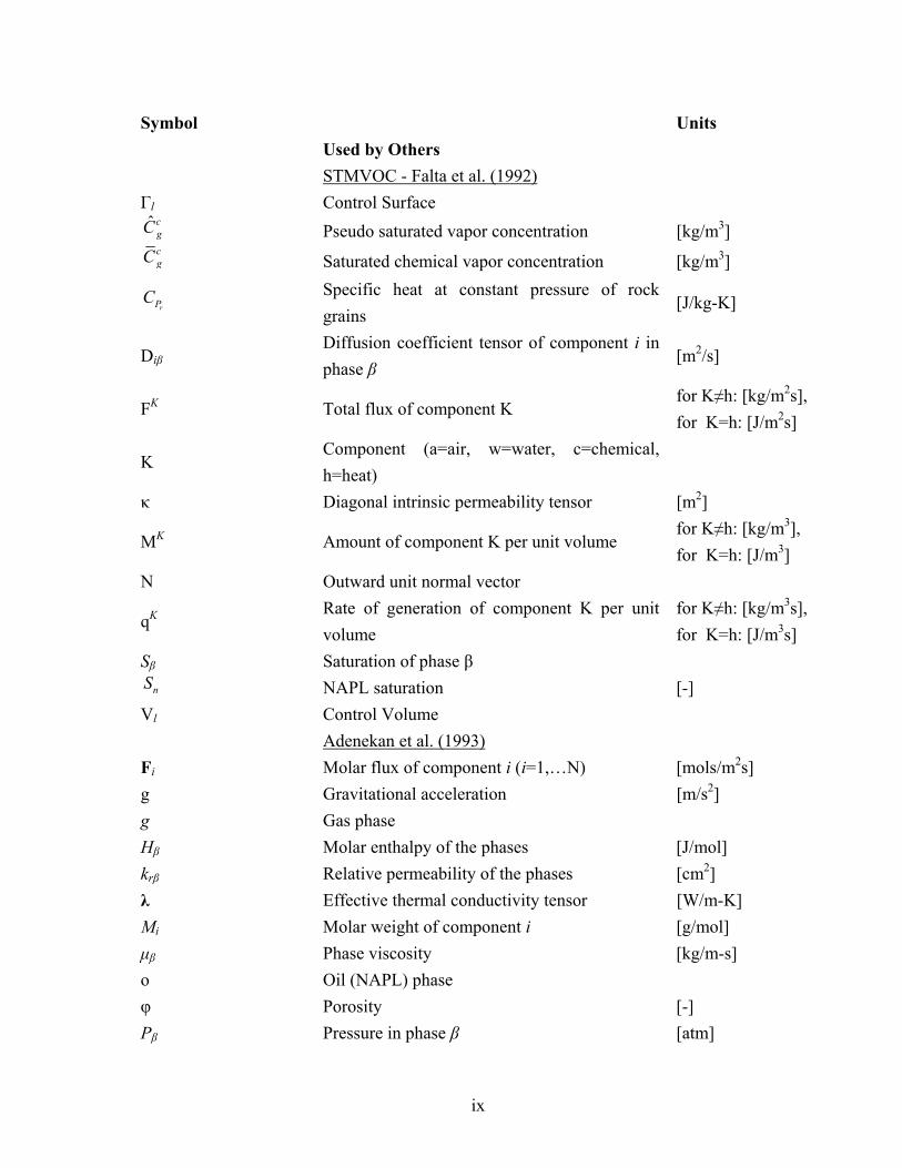
Symbol Units Used by Others STMVOC - Falta et al. (1992) Γl Control Surface
ˆ cgC Pseudo saturated vapor concentration [kg/m3] cgC Saturated chemical vapor concentration [kg/m3]
rPC Specific heat at constant pressure of rock grains
[J/kg-K]
Diβ Diffusion coefficient tensor of component i in phase β
[m2/s]
FK Total flux of component K for K≠h: [kg/m2s], for K=h: [J/m2s]
K Component (a=air, w=water, c=chemical, h=heat)
κ Diagonal intrinsic permeability tensor [m2]
MK Amount of component K per unit volume for K≠h: [kg/m3], for K=h: [J/m3]
N Outward unit normal vector
qK Rate of generation of component K per unit volume
for K≠h: [kg/m3s], for K=h: [J/m3s]
Sβ Saturation of phase β nS NAPL saturation [-]
Vl Control Volume Adenekan et al. (1993) Fi Molar flux of component i (i=1,…N) [mols/m2s] g Gravitational acceleration [m/s2] g Gas phase Hβ Molar enthalpy of the phases [J/mol] krβ Relative permeability of the phases [cm2] λ Effective thermal conductivity tensor [W/m-K] Mi Molar weight of component i [g/mol] µβ Phase viscosity [kg/m-s] o Oil (NAPL) phase φ Porosity [-] Pβ Pressure in phase β [atm]

x
Symbol Units ρ′ r Mass density of rock grains [kg/m3] ρβ Phase molar density [mols/m3] ρ′ β Mass density of phases [kg/m3]
qi Generation rate of i per unit volume of porous medium
[kg/m3]
qheat Heat generation rate per unit volume [J/m3] T Temperature [K] t Time [s] τβ Tortuosity of the flow of phase β [-] Uβ Molar internal energy of the phases [J/mol] w Water phase
wir Adsorbed mass of component i per unit mass of rock grains
[kg/kg]
xiβ Mole fraction of component i in phase β [-] Buettner and Daily (1995) C Specific heat [J/kg-K] k Relative permeability [m2] ρ density [kg/m3] T Temperature [K] t Time [s] Benard et al. (2005) E Internal energy per unit volume [J/m3] g Acceleration due to gravity [m/s2] hP Enthalpy of phase p per unit mass [J/kg] ρP Bulk density of phase p [kg/m3] p phase q Conductive thermal flux [W/m2] Q Heat source term [W/m3] t Time [s]
Pν Specific flux of phase p [m/s]

1
CHAPTER I
INTRODUCTION
1.1 Overview
Groundwater contamination by chlorinated solvents poses a serious threat to public
health. In the 2002 Agency for Toxic Substances and Disease Registry (ASTDR) Annual
Report, it was reported that more than 1.7 million people live within one mile of the 371
contaminated sites they studied. Volatile organic compounds (VOCs), including
trichloroethylene (TCE), were found at approximately 20% of the sites assessed. TCE
was most commonly used as an industrial degreaser for metal parts and was also used in
typewriter correction fluids, paint removers, and adhesives (ASTDR, 2003). TCE is a
probable human carcinogen with known acute and chronic central nervous system effects
(United States Environmental Protection Agency [EPA], 2000).
Soil vapor extraction (SVE) is the most widely known and accepted method for
vadose zone remediation at sites contaminated by TCE and other volatile chlorinated
solvents. The proven performance of SVE and availability of equipment makes SVE an
attractive remediation method for contamination in the vadose zone. However,
concentration reductions of more than 90% are difficult to achieve and treatment times
can range from six months to several years (EPA, 2000). Additionally, SVE can be used
effectively only for contaminants with vapor pressures greater than 0.1 to 1.0 mm Hg at
20°C, hydraulic conductivities greater than 1x10⁻³ to 1x10⁻² cm/s and Henry’s Law
constants greater than 100 atm per mole fraction (EPA, 1997).

2
Combining SVE with other technologies can extend the applicability of traditional
SVE. Enhancements for SVE include as air sparging, dual phase extraction, hydraulic or
pneumatic fracturing and thermal treatments (EPA, 1997). Thermal treatments include
steam and hot air injection, radiowave, microwave, electrical resistance and thermal
conduction heating. Heating the subsurface has two direct benefits: (1) increased vapor
pressure of contaminants and (2) increased air permeability achieved through soil drying.
The inspiration of thermal SVE for remediation came from the petroleum industry’s
use of steam injection since the 1980s to recover petroleum products from subsurface
formations. Other heating methods have been adapted from petroleum recovery
approaches for application to thermally-enhanced SVE. Radiowave, microwave and
electrical resistance have been used since the 1970s to extract bitumen from tar sand
deposits (Acierno et al., 2003; Kawala and Atamanczuk, 1998). Thermal SVE has
become popular in the past decade to reduce the time required for remediation, remove
sorbed compounds with low vapor pressure, solubilize or vaporize non-aqueous phase
liquids (NAPLs) and enhance biological activity (EPA, 1997).
1.2 Thesis Goals and Objectives
Although thermally-enhanced SVE has been studied for the past decade, very few
studies have addressed heating technologies other than steam injection. Electrical
resistance heating has been gaining momentum over the past few years as the preferred
enhancement method for remediation in low permeability soils. The goal of this thesis is
to formulate a general mass transfer model to simulate the SVE process augmented by
electrical resistance heating. The specific objectives of this thesis are to:

3
• Develop a conceptual model detailing the processes occurring in the vadose zone
during vapor extraction with soil heating by electrical resistance; and
• Use the conceptual model to develop a set of governing equations describing
subsurface contaminant mass transfer during vapor extraction with soil heating by
electrical resistance.
Specific tasks involved in addressing these objectives include: (1) developing a
rubric to guide decisionmakers in selecting the most appropriate thermal enhancement for
a given area, (2) deriving the appropriate multiphase equations for conservation of mass,
momentum and energy, including representing heat flux due to evaporation and
condensation processes, mass flux and convection and conduction processes, (3)
contaminant mass transfer above the boiling point of the contaminant and water, (4)
determining the appropriate simplifying assumptions.

4
CHAPTER II
LITERATURE REVIEW
2.1 Overview of Heating Techniques and Applications
The petroleum industry has been using subsurface thermal treatment for several
decades as an enhanced oil recovery technique. Thermal recovery methods for in-situ
recovery of oil are primarily used for viscosity reduction of the product (Dablow III et al.,
2000; Chute and Vermeulen, 1988; EPA, 2004). Thermal enhancement by steam
injection uses the injection pressures to mobilize petroleum products, such as crude oil,
for extraction. However, heterogeneities within the reservoir may reduce the
effectiveness of steam enhancement (Chute and Vermeulen, 1988). For this reason,
electromagnetic heating has also been used as a thermal recovery method.
Electromagnetic heating has been used to successfully extract bitumen from tar sand
deposits (Acierno et al., 2003; Kawala and Atamanczuk, 1998). Radiofrequency heating
has also been used to recover oil from oil shale with some success (Edelstein et al., 1994;
Dwyer et al., 1979; Bridges et al., 1979; Dev et al., 1989).
The first implementation of steam heating for remediation occurred in the mid-
1980s in the Netherlands (Dablow III et al., 2000). Steam injection in combination with
soil vapor extraction (SVE) has been used extensively since that time as a thermal
enhancement for subsurface remediation. Electrical resistance heating became
commercially available in 1997 and has been demonstrated at more than 30 sites in the
United States since 1999 (Beyke and Fleming, 2005). Radiofrequency heating was

5
successfully demonstrated at several sites beginning in the 1990s (Daniel et al., 1999).
Microwave enhanced remediation has been verified as a plausible thermal enhancement
in several lab-scale experiments to date (Kawala and Atamanczuk, 1998; Acierno et al.,
2003; Di et al., 2002).
Contaminants that have vapor pressures of 10 mm Hg or greater in the
temperature range required for remediation are suitable for electrical heating, including
radiofrequency heating (RFH) (Sresty, 1994). For example, trichloroethylene (TCE) and
tetrachloroethane (PCE) are both suitable for electrical heating while methylene chloride
and 1,1-Dichloroethylene (1,1-DCE) are not due to their low vapor pressures even at
increased temperatures. Figure 2-1 shows the relationship between vapor pressure and
temperature for TCE, PCE, 1, 1-DCE and methylene chloride (CRC, 1990).
0
100
200
300
400
500
600
700
800
-100 -50 0 50 100 150
Temperature (°C)
Pres
sure
(mm
Hg)
Methylene chloride1, 1-DCETCEPCE
Figure 2-1: Vapor Pressure and Temperature for Selected Compounds

6
Contaminants with vapor pressures greater than 70 Pa at 25°C are applicable for
remediation by soil vapor extraction based on prior field studies (Poppendieck et al,
1999). Vapor pressures of 70 Pa can be achieved at 150°C for up to 20 straight-chain
carbons (Schwarzenbach et al., 1993; Poppendieck et al., 1999). Temperatures in the
150°C to 200°C range can extend the minimum vapor pressure requirement from 10 mm
Hg to as low as 5 mm Hg (EPA, 1997).
2.1.1 Steam and Hot Air Injection
SVE enhanced with steam injection uses saturated steam at pressures high enough
to penetrate the pores but low enough not to exceed the fracturing pressure (EPA, 2004).
Fracturing can create channels for preferential flow where contaminated regions are not
accessed. Depending on soil permeability, steam is injected at intervals from every few
meters to more than ten meters (EPA, 2004; Davis, 1998).
Steam injected into a contaminated region enhances traditional SVE by driving
contaminants toward vapor extraction wells (Figure 2-1). Steam forms when soil and
pore fluids adjacent to the injection well reach the boiling point of water and the in-situ
vapor pressure equals that of the sum of the fluid vapor pressures (EPA, 2004; Sleep and
Ma, 1997). As the advancing edge of the steam front moves toward the extraction well,
fluids including NAPLs are volatilized from the aqueous to vapor phase; resulting in a
high concentration of vaporized contaminants behind the front (EPA, 2004).
Soils of moderate to high permeability, such as sands and gravels, are required for
successful application of steam in the vadose zone. In addition, a layer of low
permeability or confining layer below the contaminated zone is needed to prevent

7
downward contaminant migration to uncontaminated areas (EPA, 1997). Low
permeability materials, such as clay-rich soils, do not allow the steam to move easily into
the pores, resulting in ineffective heating (EPA, 1997).
Heterogeneities create a number of problematic conditions during steam flushing.
Areas layered with impermeable and permeable regions may see the extent of
contamination increased as the contaminants move along the permeable region (EPA,
1997). Preferential flow channeling around contaminated low-permeability regions of
the subsurface is also a concern when heterogeneities are present (EPA, 1997; EPA,
2004).
Figure 2-1: Steam Injection Schematic

8
Techniques that increase permeability, such as pneumatic fracturing, could be used
in combination with steam injection to improve efficiency. Care must be taken with any
permeability-enhancing technique to avoid remobilizing the contaminant downward to
uncontaminated areas. Additionally, techniques for lower permeability regions, such as
radiofrequency and electrical resistance heating, can also be used in combination with
steam injection for targeted heating of low-permeability regions.
Hot air injection is similar to enhancement by steam injection but lower in cost.
The heat capacity of air, however, is approximately four times less than that of steam, so
higher flow rates are needed for hot air injection to achieve the same heating rate as
steam injection. The vaporization/condensation process provides further heating in the
steam injection process (EPA, 2004). Enhancement by hot air injection suffers the same
stratigraphy limitations as steam injection.
2.1.2 Radio and Microwave Frequency
Radiofrequency heating (RFH) uses electrodes embedded in the soil to deliver
electromagnetic energy which enhances SVE by increasing the vapor pressure of the
contaminant, increasing soil permeability due to drying and decreasing viscosity. In a
typical installation, electrodes are placed in rows of three, with two rows acting as ground
electrodes. Electromagnetic energy is delivered to the third, which is placed between the
ground rows (Van Deuren et al., 2002). One advantage to using RFH over other
techniques is that this method is capable of heating soils to temperatures of at least 150°C
to 200°C (Van Deuren et al., 2002; EPA, 1997). Temperatures of 300°C to 400°C are

9
believed to the upper range of achievable temperatures using RFH (Dev, 1993; Sresty,
1994) though temperatures in this range have not been demonstrated.
A RFH system consists of an RF generator, matching network,
electrode/applicators, one or more antennae, temperature measuring devices, and an RF
shield (EPA, 1997; Daniel et al. 1999). An RF generator transmits energy to the
electrodes or antenna applicators (Price et al., 1999). Three phase alternating current
power, which is commercially available from the local power utility in the United States,
is converted into RF energy by a generator. A simple schematic of an RF enhanced soil
vapor extraction system is shown in Figure 2-2.
Figure 2-2: Radiofequency Heating Schematic

10
RF generators provide power, up to 25 kW, to a radiofrequency applicator which
provides a continuous RF waves at several different frequencies approved, 6.78, 13.56,
27.12, or 40.68 Hz, for industrial, scientific and medical applications (EPA, 1997; Price
et al., 1999). The frequency used is based on soil electrical properties, such as dielectric
constant and electrical conductivity (Daniel et al., 1999; EPA, 1997; Price et al., 1999).
The dielectric constant and the conductivity directly relate to the optimal wavelength and
the soil’s ability to absorb RF waves (Price et al., 1999). Matching networks modify the
RF energy to maximize the efficiency of the power absorption based on soil properties
(EPA, 1997). Energy is radiated into the soil by electrodes or antennae applicators.
Thermocouples or other temperature measuring devices are placed in the soil to monitor
heating. An RF shield may be needed if too much magnetic energy is escaping from the
treatment area (EPA, 1997).
Managing proper moisture content is critical for RFH to be implemented
effectively. Moisture is needed for radiofrequency waves to be absorbed by the soil.
However, soils that are dry or become very dry during heating will cause the impedance
to rise considerably and RF waves to not propagate sufficiently through the subsurface
(Edelstein et al., 1994). Wet soils require significantly more RF energy to heat the soil to
temperatures above 100°C (Daniel et al., 1999). Therefore, RFH has a greater potential
than steam or hot water injection in low permeability soils such as clay; clay soils
typically have higher water contents than other soils, allowing for more rapid heating and
higher attainable temperatures (Davis, 1997).

11
Microwave heating is analogous to radiofrequency heating. Microwave heating
uses electromagnetic waves with a wavelength of 1 mm to 1 m and a frequency between
300 MHz and 300 GHz; industrial and scientific applications typically use a frequency of
2.45 GHz (Acierno et al., 2003; Jones et al., 2002). Microwave induced steam distillation
(MISD) has been studied by only a few authors (Di et al., 2002; Acierno et al., 2003;
Kawala and Atamanczuk, 1998). Laboratory experiments have shown that heating is the
most intense for polar substances, for which temperatures of 100°C are achievable
(Kawala and Atamanczuk, 1998). Soil electrical properties and the applied frequency
determine the rate of heat generation (Acierno et al., 2003; Kawala and Atamanczuk,
1998). A microwave applicator for MISD has been developed by Acierno et al. (2004) in
a recent pilot study; however, this study is the only field scale study done to date.
2.1.3 Electrical Resistance
Similar to RFH, electrical resistance heating (ERH) applies heat directly to a
contaminated zone within regions of low permeability. During ERH, an electrical current
is passed through soil resulting in the generation of heat from the energy dissipated due to
the resistance provided by the porous media. A schematic of a typical ERH system is
shown in Figure 2-3.
As temperatures rise in the subsurface contaminants are vaporized and steam is
generated. ERH, like RFH, is limited by soil moisture content. The soil nearest
an electrode dries much faster than the bulk soil which leads to increased resistance to
energy flow and decreased removal efficiency (EPA, 1997). However, this decrease in
efficiency can be overcome with the addition of an aqueous solution containing an

12
electrolyte (EPA, 2004; EPA, 1997). Soil characteristics determine the rate of water and
electrolyte application required to maintain adequate moisture content. ERH is capable
of heating the soil up to 100°C; however, there is some evidence that temperatures up to
200°C may be possible (Dablow III et al., 2000).
Energy is supplied to the system directly from a power line in the form of three-
phase electricity. Six-phase power may also be used by splitting three-phase electricity.
Six-phase systems exhibit a more uniform heating distribution than three-phase systems;
however, the costs associated with converting six-phase electricity may not be worth the
increase in uniformity (Buettner and Daily, 1995). For six-phase heating, a trailer-
mounted power plant containing a transformer is needed to covert three-phase powerline
Figure 2-3: Electrical Resistance Heating System Schematic

13
frequency energy (EPA, 1997). The transformer also allows energy input to be controlled
as the resistance changes due to decreasing water content. Six-phase heating is typically
used in pilot scale applications, while three-phase electricity is preferred for full scale
operations (Beyke and Fleming, 2005). For either system, each phase is delivered to a
single electrode. Electrical phases are shifted to avoid “cold spots” between adjacent
electrodes (Buettner and Daily, 1995). In total, six electrodes are used, arranged in a
hexagonal pattern with a single SVE well in the center as shown the ERH system
schematic, Figure 2-4, below.
Typical spacing between electrodes ranges from 14 to 24 feet (Beyke and
Fleming, 2005). Treatment by ERH usually consists of several overlapping heating
arrays with diameters of 30 to 40 feet; however, single arrays of up to 100 feet in
diameter can be used (EPA, 2004; Beyke, 1998). The electrical conductivity of the soil
Figure 2-4: Electrical Resistance Heating Electrode Layout

14
limits the radius of the array (Heine and Steckler, 1999). Voltages can range between
200 and 1,600 volts depending on soil moisture content (EPA, 1997).
2.1.4 Summary and Conclusions
2.1.4.1 Generalized Costs
According to the Remediation Technologies Screening Matrix and Reference
Guide, the cost for a thermally enhanced SVE system is approximately $30 to $130 per
m3 of soil treated (Van Deuren et al., 2002). Additional cost data available varies widely
for each technology. Recent work done by Beyke and Flemming indicates that a 99%
reduction of TCE in soil and groundwater using ERH will cost $200,000 plus an
additional $50 to $100 per m3 Steam injection is estimated to be in the range of $30 to
$60 per m3. Cost information available for RFH suggests that it is in the upper end of the
range reported by Van Deuren et al. (2002). Other sources suggest the cost is somewhat
higher. Daniel et al. studied two cases where the unit cost was $182 and $288 per m3
(1999). The figures reported by Daniel et al. account for a number of parameters that
may not be included in other sources.
2.1.4.2 Recommendations and Decisionmaking
Steam Injection
Thermally enhanced soil vapor extraction using steam injection is a well
established technology. However, site geology is a significant limiting factor. Steam
injection is only applicable to sites with moderate to high permeability. Additionally, a

15
region of low permeability must be present below the zone of contamination to prevent
contaminant migration. For shallow applications, a low permeability layer near the
surface may be required to prevent steam breakthrough. Soil temperatures will be near
the boiling point of water.
Hot Air Injection
Hot air injection is relatively inexpensive. However, hot air injection is not an
efficient process due to the comparatively low heat capacity of air
Radiofrequency Heating
RFH is capable of rapidly heating soil to temperatures ranging from 150°C to
200°C. Heating with radiofrequency is comparatively uniform. RFH is well suited for
use in low permeability soils because heat is applied directly to the soil. However, such
high temperatures can lead to problems associated with soil desiccation, such as
fracturing.
Electrical Resistance Heating
ERH is well suited for use in low permeability soils because heat is applied
directly to the soil. Electrodes require little disturbance to the soil. Energy required can
be supplied directly from a local utility. ERH can heat soil to around 100ºC. ERH
depends on soil moisture content and soil drying may be problematic.
Recommendations
Based on these factors, a flow chart was developed to help decision-makers in
determining what thermal enhancement methods are applicable for a particular site.

16
Radiofrequency††
Permeability (Soil Type)
None to Low
High
Steam Injection with RF
Steam Injection with RF
High (Sands, Gravels)
Low (Clays, Silts)
†- choose the highest boiling point of all contaminants ††- water addition may be needed at sites with low moisture content Figure 2-6: Decision Tool for Selecting Most Appropriate Heating Technique
Heterogeneity
Contaminant Boiling Point†
or Desired Temperature
Below 100°C
Heterogeneity
None to Low
High
Steam Injection with ERH
Permeability (Soil Type)
High (Sands, Gravels)
Steam Injection
Low (Clays, Silts)
Electrical Resistance††
Above 100°C

17
2.2 Previous Approaches and Modeling Modeling of heat and mass transfer within a porous media has been studied by
numerous authors. Only the most relevant previous work is surveyed here. Numerical
modeling of steam injection in shallow applications has been studied at length by Falta et
al. (1992). The authors developed STMVOC a three phase (gas, liquid, NAPL) three
component system (air, water, NAPL). This simulator allows for each phase to flow.
Three mass balance equations, one energy balance equation and a set of primary and
secondary variables are used to describe the system. The key assumptions used in the
formulation of STMVOC are outlined as follows:
• Local chemical and thermal equilibrium exists between the three phases,
• No chemical reactions are occurring except mass transfer and adsorption,
• Mass transfer in the NAPL phase includes evaporation and boiling,
• Mass transfer by condensation and dissolution are also considered,
• Both the latent and sensible heat are considered to account for phase transitions.
The governing balance equations are generally written for a flow region, Vl, with a
surface area Γl:
V Γ V
V = F n Γ + Vl l l
K K Kl l lM d d q d
t∂
⋅∂ ∫ ∫ ∫ 2-1
The method of Abriola and Pinder (1985) was used to prevent complete
disappearance or appearance of a phase due to the complexity of the
appearance/disappearance mechanisms. This method uses a minimum saturation
value for the NAPL phase of 10-4. The minimum saturation is used in combination with
“pseudo” gas phase NAPL concentration which limits evaporation.

18
4ˆ
10c cng g
n
SC CS −
⎛ ⎞≈ ⎜ ⎟+⎝ ⎠
2-2
Incorporating Henry’s constant with equation 2-2 prevents complete disappearance of
the NAPL phase. The authors believe the simplicity of this method overrides the
inability to completely characterize NAPL removal. Finally, STMVOC is solved using
MULKOM (Press, 1983; 1987). MULKOM is a general integral finite difference solver
designed for multiphase heat and mass transport.
Adenekan et al. (1993) developed M2NOTS, a numerical simulator for
multicomponent multiphase transport of contaminants and heat from an injection source.
Unlike the previous work by Falta et al. (1992), the model presented allows for the
complete appearance/disappearance of each phase and any component can partition into
any fluid phase present. This simulator also accounts for three flowing phases (air, water,
NAPL), like the previous work by Falta et al. (1992). The primary assumptions made
are:
• Local chemical and thermal equilibrium,
• Multiphase fluid flow is sufficiently described by the Darcy equation,
• Gravitational and viscous forces are neglected in the energy balance,
• Adsorption follows a linear isotherm,
• No chemical reactions are occurring.
The set of governing equations presented are conservation of mass for each component,
energy balance and Darcy’s Law. The conservation of mass is:
( ), ,
1 r iri i i
w o gi
w S x qt M β β β
β
ρϕ ϕ ρ=
⎡ ⎤′∂− + = −∇ ⋅ +⎢ ⎥∂ ⎣ ⎦
∑ F 2-3

19
The energy balance is:
( )
( )
, ,
, ,
1
rr pw o g
rheat
w o g
C T S Ut
kH P T q
β β ββ
ββ β β β
β β
ϕ ρ ϕ ρ
κρ ρ
µ
=
=
⎡ ⎤∂ ′ ′− +⎢ ⎥∂ ⎣ ⎦⎡ ⎤
′= −∇ ⋅ ⋅ ∇ − + ⋅∇ +⎢ ⎥⎢ ⎥⎣ ⎦
∑
∑ g λ
2-4
Darcy’s law is written as:
( ) i, ,
Dri i i
w o g
kx P S xβ
β β β β β β β β ββ β
κρ ρ ϕ τ ρ
µ=
⎡ ⎤′= − ⋅ ∇ − + ⋅∇⎢ ⎥
⎢ ⎥⎣ ⎦∑F g 2-5
The integral finite difference method is used to solve the system of equations by
discretizing the flow domain into arbitrarily shaped polyhedrons.
A proof of concept demonstration of electrical heating completed in the summer of
1992 was modeled by Buettner and Daily (1995). The simplistic model is based on a
generic heat equation with a heat source term.
2T k UTt C Cρ ρ
⎛ ⎞∂= ∇ +⎜ ⎟∂ ⎝ ⎠
2-6
The source term is based on the electrical conductivity of the soil and the electric field
applied. This simplistic method allows the initial heating rates to be studied. The authors
make the argument that at early time the temperature will vary linearly with time.
Calculations are carried out for a three-phase system and a six-phase electrical system.
The results show that the heating-rate distribution during the first 10 days shows, as
discussed in Section 2.1.3, six-phase heating is somewhat more uniform than heating
with three-phase power.
Electrical heating has been studied on a laboratory scale by Heron et al. (1998). In
this study, the effect of heating soil to near the boiling point of TCE (85°C) and water

20
(100°C) to enhance remediation was demonstrated. Soil temperature reached 85°C after
13 days of heating and 100°C after 34 days of heating. Striking reductions in
concentration were seen after reaching 85°C. At 100°C, steam was produced due to the
boiling of water and TCE flux reached a maximum as the soil temperature was
maintained above 99°C. Heron et al. (1998) reported that TCE flux remained high even
when the residual concentration was low. This observation indicated that tailing may be
less significant using thermally enhanced SVE rather than traditional SVE. Results
suggested that sorption is still an important mechanism, though the importance may be
somewhat reduced than with a traditional SVE system.
Electrical heating has been studied at the laboratory scale by Carrigan and Nitao
(2000). The basic ohmic heating model employs a conservation of electric charge
equation and Ohm’s law. The numerical solution of the heating model employs the
superposition of two single-phase solutions. Superposition is necessary because of the
time dependent nature of the authors set of equations. The model was used to show the
temperature distribution and uniformity of an electrical heating system. As indicated by
Buettner and Daily (1995), a six-phase system is shown to be the most uniform. Since
vapors condense outside of the heated region, the authors suggest that electrical heating
should be used in conjunction with steam injection to target liquid-phase contaminants in
areas of high permeability.
Benard et al. have studied boiling in porous media (2005). The model
developed for heat and mass transfer in porous media uses a set of governing equations
consisting of mass conservation and two energy equations based on the first and second
law of thermodynamics, Figures 2-7 and 2-8 respectively.
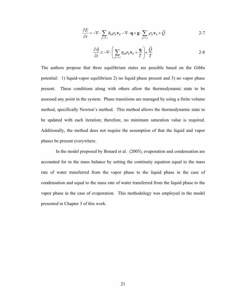
21
P P P P P, ,p l v p l v
E h Qt
ρ ρ= =
∂= −∇ ⋅ −∇ ⋅ + ⋅ +
∂ ∑ ∑ν q g ν 2-7
P P P,p l v
Qt T Tη η ρ
=
⎛ ⎞∂≥ −∇ ⋅ + +⎜ ⎟∂ ⎝ ⎠
∑ qν 2-8
The authors propose that three equilibrium states are possible based on the Gibbs
potential: 1) liquid-vapor equilibrium 2) no liquid phase present and 3) no vapor phase
present. These conditions along with others allow the thermodynamic state to be
assessed any point in the system. Phase transitions are managed by using a finite volume
method, specifically Newton’s method. This method allows the thermodynamic state to
be updated with each iteration; therefore, no minimum saturation value is required.
Additionally, the method does not require the assumption of that the liquid and vapor
phases be present everywhere.
In the model proposed by Benard et al. (2005), evaporation and condensation are
accounted for in the mass balance by setting the continuity equation equal to the mass
rate of water transferred from the vapor phase to the liquid phase in the case of
condensation and equal to the mass rate of water transferred from the liquid phase to the
vapor phase in the case of evaporation. This methodology was employed in the model
presented in Chapter 3 of this work.

22
CHAPTER III
MODEL DEVELOPMENT
3.1 Conceptual Model The symmetry of the electrical resistance heating system, shown in Figure 3-1,
allowed for the use of a representative slice – 1/6th of the circular heating array – as a
basis for examination of air flow and heat transfer within the array. The representative
slice is shown below in Figure 3-1.
Any surface from the figure above can be visualized as a section of the porous medium,
which consists of soil particles, contaminants, water and air as represented in Figure 3-2.
It is important to note that only the air phase is continuous and the solid is inert.
Figure 3-1: Representative Slice

23
The area and volume within the porous medium available for gas and liquid flow across
each surface (a thru f) in the diagram is listed in Table 3-1. The table is used extensively
in the following section in the derivations of the governing equations for conservation of
mass, momentum and energy.
Figure 3-2: Porous Medium Control Volume

24
The porous medium is conceptually represented by four separate phases – soil particle
(solid), liquid water, liquid TCE (NAPL), and gas – with interactions due to advection,
sorption, dissolution, evaporation-condensation and convection-conduction processes.
The dominant mechanisms considered here are evaporation and condensation (NAPL,
water and air components) and heat transfer by conduction and convection (all
components) illustrated in Figure 3-3. Air flow is typically saturated with respect to
water and NAPL (TCE) at a reference temperature and pressure.
Table 3-1: Flow Areas and Volumes Cross-sectional Areas for System with 4 Physical Phases
Directional Coordinate
Surface Gas Flow Liquid Flow
Total Area
r c ηθg,cr∆φ∆z ηθl,cr∆φ∆z r∆φ∆z r d ηθg,c(r+∆r)∆φ∆z ηθl,c(r+∆r)∆φ∆z (r+∆r)∆φ∆z φ a ηθg,c∆r∆z ηθl,c∆r∆z ∆r∆z φ b ηθg,c∆r∆z ηθl,c∆r∆ z ∆r∆z z e ηθg,cr∆r∆φ ηθl,cr∆r∆φ r∆r∆φ z f ηθg,cr∆r∆φ ηθl,cr∆r∆φ r∆r∆φ Volume ηθg,cr∆r∆φ∆z ηθl,cr∆r∆φ∆z r∆r∆φ∆z
Figure 3-3: Conceptual Representation of the Phases and Their Interactions

25
Water and contaminants are vaporized as the temperature near the electrode reaches the
boiling point. The vapors are then pushed toward the extraction well (rw) by the flowing
air phase as illustrated in Figure 3-4.
When the vapors reach cooler regions the NAPL and water will condense and then be
reheated as the temperature profile extends toward the vapor extraction well. This
process occurs repeatedly until the entire circular area is heated thoroughly and vapors
are removed at the vapor extraction well. Figure 3-5 demonstrates the temperature
profile expected throughout the region.
Figure 3-4: Radial Flow within the Porous Medium

26
This process results in a “hot” area of low water content behind the condensation front (Figure 3-6).
Figure 3-5: Temperature Profile
Figure 3-6: Moisture Content along the Radial Axis

27
The pressure distribution, illustrated in Figure 3-7, increases with radial distance.
3.2 Governing Equations
Governing equations for the conservation of mass, momentum and energy are
derived for the most general case following the shell balance approach of Bird, Stewart
and Lightfoot (1960). Then, the general equations are written for a multiphase
multicomponent system according to Table 3-2, which illustrates possible phase-
component combinations.
Figure 3-7: Pressure Profile

28
The following assumptions were made in the derivation of each conservation
equation. The gas phase is compressible and the ideal gas law applies. The liquid phase
is incompressible and immobile. The solid is considered to be inert – sorption is not
considered. The air phase is composed primarily of nitrogen; therefore, physical
properties of air will be based on N2. The thickness of the porous medium is constant.
The porosity is constant. Several additional assumptions were made for the conservation
of energy equation. The system is nonisothermal, nonadiabatic, nonisentropic. Local
thermal equilibrium (i.e., Ts=TNAPL=Tair=Twater) is assumed (Falta et al., 1992; Adenekan
et al., 1993; Benard et al., 2005). Viscous forces are negligible in comparison to the heat
transfer process (Adenekan et al., 1993). Internal energy is much larger than kinetic
energy; therefore, kinetic energy is neglected. Potential energy is assumed negligible as
well (Adenekan et al., 1993).
Table 3-2: Phase-Component Possibilities Phase (β) Liquid Gas Solid Component (α) soil X air X TCE X (NAPL) X water X X X denotes phase-component combination

29
3.2.1 Conservation of Mass
The governing conservation of mass equation is derived from applying the
Reynolds Transport Theorem over a differential control volume:
ηθρ dV ρ(ν n) dA= VCV CS
mt∂
+ ⋅∂ ∫∫∫ ∫∫ (3.1)
Integrations are performed over the entire differential control volume and control surface
as shown in Figures 3.3 and 3.1, respectively.
a a b b c c d d e e f fηθρV ρ( A A A A A A ) Vmt∂
+ − + − + − + =∂
ν ν ν ν ν ν (3.2)
Volume, area and velocity components from Table 3.1 are substituted into the above
equation
( )
φφ φ
rr r
zz z
ρηθρ(ηθr∆r∆φ∆z) ηθ∆r∆z ρ+ ρt t
ρ +ηθ∆φ∆z r ∆r ρ+ rρt t
ρ +ηθr∆r∆z ρ+ ρ (ηθr∆r∆φ∆z)t t
t
m
⎡ ⎤∂⎛ ⎞∂ ∂⎛ ⎞+ + −⎢ ⎥⎜ ⎟⎜ ⎟∂ ∂ ∂⎝ ⎠⎝ ⎠⎣ ⎦⎡ ⎤∂∂ ⎛ ⎞⎛ ⎞+ + −⎜ ⎟⎜ ⎟⎢ ⎥∂ ∂⎝ ⎠⎝ ⎠⎣ ⎦⎡ ⎤∂∂ ⎛ ⎞⎛ ⎞ + − =⎜ ⎟⎜ ⎟⎢ ⎥∂ ∂⎝ ⎠⎝ ⎠⎣ ⎦
νν ν
νν ν
νν ν
(3.3)
The relationship is divided by volume ( )ηθr∆r∆φ∆z and the limit as ∆r, ∆φ, and ∆z
approach zero is taken to obtain
r φ z1 1ηθρ (rρ ) (ρ ) (ρ )r r r φ z
mt∂ ∂ ∂ ∂
+ + + =∂ ∂ ∂ ∂
ν ν ν (3.4)
which can be rewritten as the equation of continuity
ηθρ ( ρ ) mt∂
+ ∇⋅ =∂
ν (3.5)

30
The rate of mass transferred per unit volume per time ( m ) is
vaph
m = ±q (3.6)
where (+) indicates evaporation and (-) indicates condensation. For a multicomponent
multiphase system the governing equation for conservation of mass is:
, , ,vap
ηθ ρ ( )ht α β α β α β
∂+ ∇ ⋅ = ±
∂qν (3.7)
For the components TCE, air, and water, the equation for conservation of mass in the gas
phase is:
2 2 2 2; , , ; , , ; , , ; , ,
vap
ηθ ρ ( ρ )hg TCE N water g TCE N water g TCE N water g TCE N watert
∂+ ∇ ⋅ = ±
∂qν (3.8)
Since the liquid phase is immobile in this system ( 0l =ν ), conservation of mass is
written as:
2 2; , , ; , ,
vap
ηθ ρhl TCE N water l TCE N watert
∂= ±
∂q (3.9)
3.2.2 Conservation of Momentum
Similarly, the governing equation for conservation of mass is derived from the
Reynolds Transport Theorem applied to the differential control volume shown in Figure
3.1:
ρ dV ρ( ) dA FCV CS
nt
ν∂+ ⋅ =
∂ ∑∫∫∫ ∫∫ν ν (3.10)
Integrating over the differential control volume and control surface for the gas phase as
shown in Figures 3.3 and 3.1, respectively:

31
( ) ( ) g P va a b b c c d d e e f fρ dV ρ A A A A A A =F - F - Ft∂
+ − + − + − +∂
ν ν ν ν ν ν ν ν (3.11)
Volume, area and velocity components from Table 3.1 can be substituted into the above
equation
( )
( )
φφ φ
rr r
zz z g P v
ρηθr∆r∆φ∆z ρ∆r∆zηθφ
ρ∆φ∆zηθ r+∆r rr
ρr∆r∆φηθ F + F + Fz
t
⎡ ⎤⎛ ⎞∂∂+ + −⎢ ⎥⎜ ⎟⎜ ⎟∂ ∂⎢ ⎥⎝ ⎠⎣ ⎦
⎡ ⎤⎛ ⎞∂+ −⎢ ⎥⎜ ⎟∂⎝ ⎠⎣ ⎦
⎡ ⎤⎛ ⎞∂+ + − =⎢ ⎥⎜ ⎟∂⎝ ⎠⎣ ⎦
νν ν ν ν
ν+ ν ν ν
νν ν ν
(3.12)
The relationships for the forces are gF ρ dV
CV
= ∫∫∫ g (gravity) (3.13)
PF P dA
CS
= ∫∫ (pressure) (3.14)
( )vF dA
CS
n= ⋅∫∫ τ (viscous) (3.15)
Performing the integrations in (3.13), (3.14), and (3.15) gF ρ r∆r∆φ∆z= g (3.16)
P a a b b c c d d e e f fF = -P A + P A P A + P A P A + P A− − (3.17)
v a a b b c c d d e e f fF = - A + A - A + A - A + Aτ τ τ τ τ τ (3.18)

32
Pressure and area over the control surface can be substituted into (3.17).
( )φ r
P φ φ r r
zz z
P PF = ∆r∆z P P +∆φ∆z r+∆r P rPφ r
P r∆r∆φ P Pz
⎡ ⎤⎛ ⎞ ⎡ ⎤∂ ⎛ ⎞∂+ − + −⎢ ⎥⎜ ⎟ ⎢ ⎥⎜ ⎟⎜ ⎟∂ ∂⎢ ⎥ ⎝ ⎠⎣ ⎦⎝ ⎠⎣ ⎦
⎡ ⎤⎛ ⎞∂+ + −⎢ ⎥⎜ ⎟∂⎝ ⎠⎣ ⎦
(3.19)
Viscous forces and area for the control surface can be substituted into (3.18).
( ) ( ) ( )rφrr rzv rr rr rφ rφ rz rz
φr φφ φzφr φr φφ φφ φz φz
F = ∆φ∆z r+∆r r r+∆r r r+∆r rr r r
+∆r∆zφ φ φ
τ⎡ ⎤∂⎧ ⎫⎛ ⎞⎡ ⎤ ⎡ ⎤∂ ∂⎛ ⎞ ⎛ ⎞+ − + + − + + −⎨ ⎬⎢ ⎥⎜ ⎟⎜ ⎟ ⎜ ⎟⎢ ⎥ ⎢ ⎥∂ ∂ ∂⎝ ⎠ ⎝ ⎠⎣ ⎦ ⎣ ⎦⎝ ⎠⎩ ⎭⎣ ⎦
⎧⎡ ⎤ ⎡ ⎤ ⎡∂ ∂ ∂⎛ ⎞ ⎛ ⎞ ⎛ ⎞⎪ + − + + − + + −⎨⎢ ⎥ ⎢ ⎥⎜ ⎟ ⎜ ⎟ ⎜ ⎟∂ ∂ ∂⎝ ⎠ ⎝ ⎠ ⎝ ⎠⎪⎣ ⎦ ⎣ ⎦⎩
ττ ττ τ τ τ τ
τ τ ττ τ τ τ τ τ
zφzr zzzr zr zφ zφ zz zz
r∆r∆φφ z φ
τ
⎫⎤⎪⎬⎢ ⎥⎪⎣ ⎦⎭
⎧ ⎫⎡ ⎤∂⎡ ⎤ ⎡ ⎤⎛ ⎞⎛ ⎞ ⎛ ⎞∂ ∂⎪ ⎪+ + − + + − + + −⎨ ⎬⎢ ⎥⎢ ⎥ ⎢ ⎥⎜ ⎟⎜ ⎟ ⎜ ⎟∂ ∂ ∂⎝ ⎠ ⎝ ⎠⎪ ⎪⎝ ⎠⎣ ⎦ ⎣ ⎦⎣ ⎦⎩ ⎭
τττ τ τ τ τ τ
(3.20)
The relationships for gravitational, pressure and viscous forces [(3.16), (3.19) and (3.20)]
are substituted into right hand side of equation (3.12).

33
( )
( )
( )
φφ φ
r zr r z z
φφ φ
ε r
ρηθr∆r∆φ∆z ρ ∆r∆zηθφ
∆φ∆zηθ r+∆r r r∆r∆φηθr z
P ρ r∆r∆φ∆z ∆r∆z P P
φ
P ∆φ∆z r+∆r Prr
t
⎧ ⎡ ⎤⎛ ⎞∂∂ ⎪+ + −⎢ ⎥⎜ ⎟⎨ ⎜ ⎟∂ ∂⎢ ⎥⎪ ⎝ ⎠⎣ ⎦⎩⎫⎡ ⎤ ⎡ ⎤⎛ ⎞ ⎛ ⎞∂ ∂ ⎪+ + − + + − ⎬⎢ ⎥ ⎢ ⎥⎜ ⎟ ⎜ ⎟∂ ∂⎝ ⎠ ⎝ ⎠ ⎪⎣ ⎦ ⎣ ⎦⎭
⎡ ⎤⎛ ⎞∂= − + −⎢ ⎥⎜ ⎟⎜ ⎟∂⎢ ⎥⎝ ⎠⎣ ⎦
⎛ ∂+ +
∂
νν ν ν ν
ν νν ν ν ν
g
( ) ( )
( )
zr z z
rφrrrr rr rφ rφ
φrrzrz rz φr φr
PrP r∆r∆ P P
∆φ∆z r+∆r r r+∆r rr r
r+∆r r ∆r∆zr φ
zφ
τ
⎡ ⎤ ⎡ ⎤⎞ ⎛ ⎞∂− + + −⎢ ⎥ ⎢ ⎥⎜ ⎟ ⎜ ⎟∂⎝ ⎠ ⎝ ⎠⎣ ⎦ ⎣ ⎦
⎡ ⎤∂⎧ ⎛ ⎞⎡ ⎤∂⎛ ⎞− + − + + −⎨ ⎢ ⎥⎜ ⎟⎜ ⎟⎢ ⎥∂ ∂⎝ ⎠⎣ ⎦ ⎝ ⎠⎩ ⎣ ⎦⎧⎡ ⎤∂⎫ ⎛ ⎞⎡ ⎤∂ ⎪⎛ ⎞+ + − + + −⎬ ⎨⎢ ⎥⎜ ⎟⎜ ⎟⎢ ⎥∂ ∂⎝ ⎠⎣ ⎦ ⎝ ⎠⎪⎭ ⎣ ⎦⎩
+
τττ τ τ τ
τττ τ τ
φφ φzφφ φφ φz φz
zφzr zzzr zr zφ zφ zz zz
φ φ
r∆r∆φφ φz
τ
⎫⎡ ⎤ ⎡ ⎤∂ ∂⎛ ⎞ ⎛ ⎞ ⎪+ − + + − ⎬⎢ ⎥ ⎢ ⎥⎜ ⎟ ⎜ ⎟∂ ∂⎝ ⎠ ⎝ ⎠ ⎪⎣ ⎦ ⎣ ⎦⎭⎧ ⎫⎡ ⎤∂⎡ ⎤ ⎡ ⎤⎛ ⎞⎛ ⎞ ⎛ ⎞∂ ∂⎪ ⎪+ + − + + − + + −⎨ ⎬⎢ ⎥⎢ ⎥ ⎢ ⎥⎜ ⎟⎜ ⎟ ⎜ ⎟∂ ∂ ∂⎝ ⎠ ⎝ ⎠⎪ ⎪⎝ ⎠⎣ ⎦ ⎣ ⎦⎣ ⎦⎩ ⎭
τ ττ τ τ τ
τττ τ τ τ τ τ
(3.21)
Dividing (3.21) by volume ( )ηθr∆r∆φ∆z and taking the limit as ∆r, ∆φ, and ∆z approach
zero:
( ) ( ) ( ) ( )
( )
( ) ( ) ( ) ( )
( ) ( ) ( ) ( ) ( )
φ z
φ zr
φrrr rφ rz
φφ φz zr zφ zz
1 1ρ rρ ρ ρr r r φ z
P Pρ 1 1 1 rPηθ ηθ r r r φ z
1 1 1 1 ηθ r r rr r r r r r r φ
1 1 r φ r φ z z z
rt⎧ ⎫∂ ∂ ∂ ∂
+ + +⎨ ⎬∂ ∂ ∂ ∂⎩ ⎭⎧ ⎫∂ ∂∂⎪ ⎪= − + +⎨ ⎬∂ ∂ ∂⎪ ⎪⎩ ⎭
⎧ ∂ ∂ ∂ ∂− + + +⎨ ∂ ∂ ∂ ∂⎩
⎫∂ ∂ ∂ ∂ ∂+ + + + + ⎬∂ ∂ ∂ ∂ ∂ ⎭
ν ν ν ν ν
g
ττ τ τ
τ τ τ τ τ
(3.22)
34
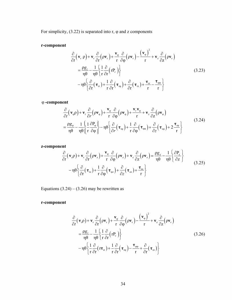
For simplicity, (3.22) is separated into r, φ and z components r-component
( ) ( ) ( ) ( ) ( )
( )
( ) ( ) ( )
2
φφr r r r z r
rr
φφrrrr rφ rz
ρ ρ ρ ρr r φ r z
ρ 1 1 rPηθ ηθ r r
1 ηθr r r r r r
tg
∂ ∂ ∂ ∂+ + − +
∂ ∂ ∂ ∂
∂⎧ ⎫= − ⎨ ⎬∂⎩ ⎭⎧ ⎫∂ ∂ ∂
− + + + −⎨ ⎬∂ ∂ ∂⎩ ⎭
ννν ν ν ν ν ν
τττ τ τ
(3.23)
φ -component
( ) ( ) ( ) ( )
( ) ( ) ( )
φ r φφ r φ φ z φ
φ φ rφφφrφ zφ
ρ ρ ρ ρr φ r z
ρ P1 1 1ηθ 2ηθ ηθ r φ r φ r
t r
gr z
∂ ∂ ∂ ∂+ + + +
∂ ∂ ∂ ∂
⎧ ⎫∂ ⎧ ⎫∂ ∂ ∂⎪ ⎪= − − + + +⎨ ⎬ ⎨ ⎬∂ ∂ ∂ ∂⎪ ⎪ ⎩ ⎭⎩ ⎭
ν ν νν ν ν ν ν ν
τττ τ
(3.24)
z-component
( ) ( ) ( ) ( )
( ) ( ) ( )
φ z zz r z z z z
rzrz φz zz
ρ P1ρ ρ ρ ρr r φ z ηθ ηθ z
1 ηθr r φ r
gt
z
⎧ ⎫∂∂ ∂ ∂ ∂+ + + = − ⎨ ⎬∂ ∂ ∂ ∂ ∂⎩ ⎭⎧ ⎫∂ ∂ ∂
− + + +⎨ ⎬∂ ∂ ∂⎩ ⎭
νν ν ν ν ν ν
ττ τ τ (3.25)
Equations (3.24) – (3.26) may be rewritten as r-component
( ) ( ) ( ) ( ) ( )
( )
( ) ( ) ( )
2
φφr r r r z r
rr
φφrr rφ rz
ρ ρ ρ ρr r φ r z
ρ 1 1 rPηθ ηθ r r
1 1 ηθ rr r r r r r
tg
∂ ∂ ∂ ∂+ + − +
∂ ∂ ∂ ∂
∂⎧ ⎫= − ⎨ ⎬∂⎩ ⎭⎧ ⎫∂ ∂ ∂
− + − +⎨ ⎬∂ ∂ ∂⎩ ⎭
ννν ν ν ν ν ν
ττ τ τ
(3.26)

35
φ -component
( ) ( ) ( ) ( )
( ) ( ) ( )
φ r φφ r φ φ z φ
φ φ
2φφrφ zφ2
ρ ρ ρ ρr r φ r z
ρ P1 1 ηθ ηθ r φ
1 1 ηθ rr r r φ
t
g
z
∂ ∂ ∂ ∂+ + + +
∂ ∂ ∂ ∂
⎧ ⎫∂⎪ ⎪= − ⎨ ⎬∂⎪ ⎪⎩ ⎭⎧ ⎫∂ ∂ ∂
− + +⎨ ⎬∂ ∂ ∂⎩ ⎭
ν ν νν ν ν ν ν ν
ττ τ
(3.27)
z-component
( ) ( ) ( ) ( )
( ) ( ) ( )
φz r z z z z
z
rz φz zz
ρ ρ ρ ρr r φ z
ρ P1 ηθ ηθ z
1 1 ηθ rr r r φ z
z
t
g
∂ ∂ ∂ ∂+ + +
∂ ∂ ∂ ∂
⎧ ⎫∂= − ⎨ ⎬∂⎩ ⎭
⎧ ⎫∂ ∂ ∂− + +⎨ ⎬∂ ∂ ∂⎩ ⎭
νν ν ν ν ν ν
τ τ τ
(3.28)
The relationships for τ as listed in (3.29), assuming the vapor phase is a Newtonian fluid
are substituted into (3.27), (3.28) and (3.29) as appropriate.
( )
( )
( )
rrr
φ rφφ
zzz
φ rrφ φr
φ zzφ φz
z rzr rz
22r 3
1 22r φ r 3
22z 3
1rr r r φ
1z r φ
zr
µ
µ
µ
τ µ
τ µ
τ µ
⎡ ⎤∂= − − ∇ ⋅⎢ ⎥∂⎣ ⎦
⎡ ⎤⎛ ⎞∂= − + − ∇ ⋅⎢ ⎥⎜ ⎟⎜ ⎟∂⎢ ⎥⎝ ⎠⎣ ⎦
⎡ ⎤∂= − − ∇ ⋅⎢ ⎥∂⎣ ⎦
⎡ ⎤⎛ ⎞ ∂∂= = − +⎢ ⎥⎜ ⎟⎜ ⎟∂ ∂⎢ ⎥⎝ ⎠⎣ ⎦
⎡ ⎤∂ ∂= = − +⎢ ⎥
∂ ∂⎢ ⎥⎣ ⎦⎡ ⎤∂ ∂
= = − +⎢ ⎥∂ ∂⎣ ⎦
ντ ν
ν ντ ν
ντ ν
ν ντ
ν ντ
ν ντ
(3.29)

36
r-component
( ) ( ) ( ) ( ) ( )
( ) ( )
( )
2
φφr r r r z r
r rr
φ φr r
ρ ρ ρ ρr φ r z
ρ 1 1 1 2 rP + ηθ r 2ηθ ηθ r r r r r 3
1 1 1 1 2 r 2r φ r r r φ r r φ r 3
t r
g µ
∂ ∂ ∂ ∂+ + − +
∂ ∂ ∂ ∂
⎧ ⎛ ⎞⎡ ⎤∂∂ ∂⎪⎧ ⎫= − − ∇ ⋅⎜ ⎟⎨ ⎬ ⎨ ⎢ ⎥⎜ ⎟∂ ∂ ∂⎩ ⎭ ⎣ ⎦⎪ ⎝ ⎠⎩⎛ ⎞⎡ ⎤ ⎡ ⎤⎛ ⎞ ⎛ ⎞∂∂∂ ∂⎜ ⎟+ + − + − ∇ ⋅⎢ ⎥ ⎢ ⎥⎜ ⎟ ⎜ ⎟⎜ ⎟ ⎜ ⎟⎜ ⎟∂ ∂ ∂ ∂⎢ ⎥ ⎢ ⎥⎝ ⎠ ⎝ ⎠⎣ ⎦ ⎣ ⎦⎝ ⎠
ννν ν ν ν ν ν
ν ν
ν νν ν ν
z r z r z
⎫⎛ ⎞⎡ ⎤∂ ∂∂ ⎪+ +⎜ ⎟⎬⎢ ⎥⎜ ⎟∂ ∂ ∂⎣ ⎦ ⎪⎝ ⎠⎭
ν ν
(3.30)
φ -component
( ) ( ) ( ) ( )
( )
φ r φφ r φ φ z φ
φ φ φ2 r2
φ φr z
ρ ρ ρ ρr r φ r z
ρ P1 1 1 1 + ηθ r rηθ ηθ r φ r r r r r φ
1 1 2 1 2r φ r φ r 3 z z r φ
t
gµ
∂ ∂ ∂ ∂+ + + +
∂ ∂ ∂ ∂
⎧ ⎛ ⎞⎡ ⎤⎧ ⎫ ⎛ ⎞∂ ∂∂ ∂⎪ ⎪ ⎪ ⎜ ⎟= − +⎢ ⎥⎜ ⎟⎨ ⎬ ⎨ ⎜ ⎟⎜ ⎟∂ ∂ ∂ ∂⎪ ⎪ ⎢ ⎥⎪⎩ ⎭ ⎝ ⎠⎣ ⎦⎝ ⎠⎩
⎛ ⎞⎡ ⎤⎛ ⎞ ⎡∂ ∂ ∂∂ ∂⎜ ⎟+ + − ∇ ⋅ + +⎢ ⎥⎜ ⎟⎜ ⎟⎜ ⎟∂ ∂ ∂ ∂ ∂⎢ ⎥⎝ ⎠ ⎣⎣ ⎦⎝ ⎠
ν ν νν ν ν ν ν ν
ν ν
ν νν νν⎫⎛ ⎞⎤ ⎪⎜ ⎟⎢ ⎥ ⎬⎜ ⎟⎢ ⎥ ⎪⎦⎝ ⎠⎭
(3.31)
z-component
( ) ( ) ( ) ( )
( )
φz r z z z z
z z z r
φ z z
ρ ρ ρ ρr r φ z
ρ P1 1 ηθ rηθ ηθ z r r r z
1 1 2 2r φ z r φ z z 3
t
g µ
∂ ∂ ∂ ∂+ + +
∂ ∂ ∂ ∂
⎧ ⎛ ⎞⎧ ⎫ ⎡ ⎤∂ ∂ ∂∂⎪= − + +⎜ ⎟⎨ ⎬ ⎨ ⎢ ⎥⎜ ⎟∂ ∂ ∂ ∂⎩ ⎭ ⎣ ⎦⎪ ⎝ ⎠⎩⎫⎛ ⎞⎡ ⎤ ⎛ ⎞∂ ⎡ ⎤∂ ∂∂ ∂ ⎪+ + + − ∇⋅⎜ ⎟⎢ ⎥ ⎜ ⎟⎬⎢ ⎥⎜ ⎟⎜ ⎟∂ ∂ ∂ ∂ ∂⎢ ⎥ ⎣ ⎦⎝ ⎠⎪⎣ ⎦⎝ ⎠ ⎭
νν ν ν ν ν ν
ν ν
ν ν ν ν
(3.32)
The indicated differentiations in (3.30), (3.31), and (3.32) are performed and each
equation is rewritten for a multicomponent multiphase system. Thus, the governing
equations for conservation of momentum are

37
r-component
( ) ( ) ( ) ( ) ( )
( ) ( )
,,
, , , , , ,
, ,
, , ,
2
φφ, r r , r , r z , r
,r , , r
, ,
2 2r φ r
2 2 2 2
ρ ρ ρ ρr r φ r z
ρ 1 1 1 rP + ηθ rηθ ηθ r r r r r
1 2 2 r φ r φ z
tg
α βα β
α β α β α β α β α β α β
α β α β
α β α β α β
α β α β α β α β
α βα β α β
α β α β
µ
∂ ∂ ∂ ∂+ + − +
∂ ∂ ∂ ∂
⎧∂ ∂ ∂⎧ ⎫ ⎡ ⎤= − ⎨ ⎬ ⎨ ⎢ ⎥∂ ∂ ∂⎩ ⎭ ⎣ ⎦⎩
⎛ ⎞∂ ∂ ∂⎜ ⎟+ − + +⎜ ⎟∂ ∂ ∂⎝ ⎠
ννν ν ν ν ν ν
ν
ν ν ν( ) ( ), ,
23r 3 rα β α β
⎫∂ ⎪∇ ⋅ − ∇ ⋅ ⎬∂ ⎪⎭ν ν
(3.33)
φ -component
( ) ( ) ( ) ( ), , ,
, , , , ,
, , , ,
, ,
φ r φ, φ r , φ , φ z , φ
2φ φ φ φ,
, , 2 2, ,
2φ r
2 2 2
ρ ρ ρ ρr r φ r z
Pρ 1 1 + ηθηθ ηθ r φ r r r
2 2 r φ r φ
t
g
α β α β α β
α β α β α β α β α β
α β α β α β α β
α β α β
α β α β α β α β
α βα β α β
α β α β
µ
∂ ∂ ∂ ∂+ + + +
∂ ∂ ∂ ∂
⎧⎧ ⎫ ⎛ ⎞∂ ∂ ∂⎪ ⎪ ⎪ ⎜ ⎟= − − +⎨ ⎬ ⎨ ⎜ ⎟∂ ∂ ∂⎪ ⎪ ⎪⎩ ⎭ ⎝ ⎠⎩
∂ ∂+ +
∂ ∂
ν ν νν ν ν ν ν ν
ν ν ν
ν ν( ),
2φ
,2
2z 3r φ
α β
α β
⎫∂ ∂ ⎪+ − ∇ ⋅ ⎬∂ ∂ ⎪⎭
νν
(3.34)
z-component
( ) ( ) ( ) ( )
( )
,
, , , , , ,
, ,
, ,
φ, z r , z , z z , z
z z,, ,
, ,
2 2z z
,2 2 2
ρ ρ ρ ρr r φ z
Pρ 1 1 + ηθ rηθ ηθ z r r r
1 2 r φ z 3
t
g
z
α β
α β α β α β α β α β α β
α β α β
α β α β
α β α β α β α β
α βα β α β
α β α β
α β
µ
∂ ∂ ∂ ∂+ + +
∂ ∂ ∂ ∂
⎧⎧ ⎫ ⎛ ⎞∂ ∂∂⎪ ⎪ ⎪ ⎜ ⎟= − ⎨ ⎬ ⎨ ⎜ ⎟∂ ∂ ∂⎪ ⎪ ⎪⎩ ⎭ ⎝ ⎠⎩⎫∂ ∂ ∂ ⎪+ + − ∇⋅ ⎬
∂ ∂ ∂ ⎪⎭
νν ν ν ν ν ν
ν
ν νν
(3.35)
Since the liquid phase is assumed to be immobile in this system, the equations for
conservation of momentum are written only for the gas phase for the components TCE,
air, and water as a single miscible phase (i.e., ideal gas).

38
r-component
( ) ( )
( ) ( )2 ; , , ; , , 2 ; , ,2 2 2
; , ,; , , 22
2 ; , ,2
; , , 22
; , , r r ; , , r
2
φφ; , , r
z ; , ,
ρ ρr
ρr φ r
ρz
g TCE N water g TCE N water g TCE N water
g TCE N waterg TCE N water
g TCE N water
g TCE N water
g TCE N water g TCE N water
g TCE N water
g TCE N wate
t∂ ∂
+∂ ∂
∂+ −
∂
∂+
∂
ν ν ν
ννν
ν ( )
( )
( )
2
; , ,22
; , ,22
2 2 ; , ,2
; , ,2
; , ,r
; , ,
r; , ,
; , , ; , , r
2r
2
ρηθ
1 1 rPηθ r r
1 + ηθ rr r r
1 r
g TCE N water
g TCE N water
g TCE N water
g TCE N water
g TCE N waterr
g TCE N water
g TCE N water
g TCE N water g TCE N water
g
µ
=
∂⎧ ⎫− ⎨ ⎬∂⎩ ⎭
⎧ ∂ ∂⎡ ⎤⎨ ⎢ ⎥∂ ∂⎣ ⎦⎩
∂+
ν
ν
ν
( ) ( )
; , , ; , ,2 2
2 2
2φ r
2 2 2
; , , ; , ,
2φ r φ z
2 2 3r 3 r
g TCE N water g TCE N water
g TCE N water g TCE N water
⎛ ⎞∂ ∂⎜ ⎟− +⎜ ⎟∂ ∂ ∂⎝ ⎠
∂ ⎫+ ∇⋅ − ∇ ⋅ ⎬∂ ⎭
ν ν
ν ν (3.36)
φ -component
( ) ( )
( )
2 ; , , ; , , 2 ; , ,2 2 2
; , , ; , , ; , ,2 2 2
2 ; , ,2
; , ,2
; , , φ r ; , , φ
φ r φ; , , φ
z
ρ ρr
ρr φ r
g TCE N water g TCE N water g TCE N water
g TCE N water g TCE N water g TCE N water
g TCE N water
g TCE N water
g TCE N water g TCE N water
g TCE N water
t∂ ∂
+∂ ∂
∂+ +
∂
∂+
∂
ν ν ν
ν ν νν
ν ( ) 2
2 ; , ,22
; , ,2
2
; , ,2
2 2
; , ,2
; , ,; , , φ
; , ,
φ
; , ,
2φ
; , , ; , , 2
φ
ρρ
z ηθ
P1 1 ηθ r φ
+ ηθr
g TCE N water
g TCE N water
g TCE N water
g TCE N
g TCE N waterg TCE N water
g TCE N water
g TCE N water
g TCE N water g TCE N water
g
µ
=
⎧ ⎫∂⎪ ⎪− ⎨ ⎬∂⎪ ⎪⎩ ⎭⎧∂⎪⎨ ∂⎪⎩
−
ν
ν
ν
( )
; , , ; , ,2 2
; , , ; , ,2 2
; , ,2
2φ φ
2 2 2
2r φ
2 2
2r r r φ
2 2 r φ z 3r φ
water g TCE N water g TCE N water
g TCE N water g TCE N water
g TCE N water
⎛ ⎞ ∂ ∂⎜ ⎟ + +⎜ ⎟ ∂ ∂⎝ ⎠
∂ ∂ ⎫∂+ + − ∇⋅ ⎬∂ ∂ ∂ ⎭
ν ν
ν νν (3.37)
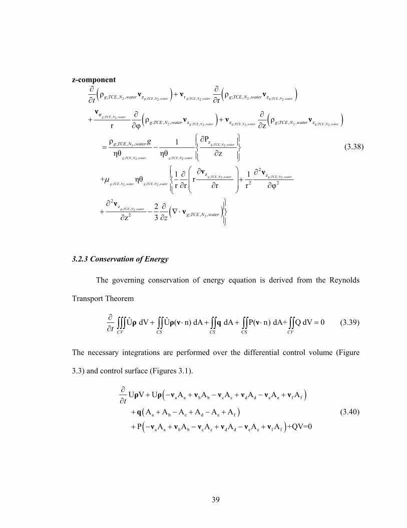
39
z-component
( ) ( )
( ) ( )
2 ; , , ; , , 2 ; , ,2 2 2
; , ,2
2 ; , , ; , , 2 ; , ,2 2 2
; , , z r ; , , z
φ
; , , z z ; , , z
;
ρ ρr
ρ ρr φ z
ρ
g TCE N water g TCE N water g TCE N water
g TCE N water
g TCE N water g TCE N water g TCE N water
g TCE N water g TCE N water
g TCE N water g TCE N water
g TC
t∂ ∂
+∂ ∂
∂ ∂+ +
∂ ∂
=
ν ν ν
νν ν ν
; , ,2 2
; , , ; , ,2 2
; , , ; , ,2 2
; , , ; , ,2 2
; , ,2
z, ,
2z z
2 2
2z
P1ηθ ηθ z
1 1 + ηθ rr r r r φ
g TCE N water
g TCE N water g TCE N water
g TCE N water g TCE N water
g TCE N water g TCE N water
g TCE N water
E N water g
µ
⎧ ⎫∂⎪ ⎪− ⎨ ⎬∂⎪ ⎪⎩ ⎭⎧ ⎛ ⎞∂ ∂∂⎪ ⎜ ⎟ +⎨ ⎜ ⎟∂ ∂ ∂⎪ ⎝ ⎠⎩
∂+
∂
ν ν
ν( )2; , ,2
2z 3 g TCE N waterz
⎫∂ ⎪− ∇ ⋅ ⎬∂ ⎪⎭ν
(3.38)
3.2.3 Conservation of Energy The governing conservation of energy equation is derived from the Reynolds
Transport Theorem
CS
ˆ ˆU dV U ( n) dA dA P( n) dA+ Q dV 0CV CS CS CVt
∂+ ⋅ + + ⋅ =
∂ ∫∫∫ ∫∫ ∫∫ ∫∫ ∫∫ρ ρ ν q ν (3.39)
The necessary integrations are performed over the differential control volume (Figure
3.3) and control surface (Figures 3.1).
( )( )( )
a a b b c c d d e e f f
a b c d e f
a a b b c c d d e e f f
U V U A A A A A A
A A A A A A
P A A A A A A +QV=0
t∂
+ − + − + − +∂
+ + − + − +
+ − + − + − +
ρ ρ ν ν ν ν ν ν
q
ν ν ν ν ν ν
(3.40)

40
Volume, area and velocity components (Table 3.1) may be substituted into the above
equation
( )
( )
( )
U θηr r φ∆z U ∆r∆zηθ
∆φ∆zηθ r+∆r r∆r∆φηθ
∆r∆zηθ ∆φ∆zηθ r+∆r
r zr r z z
rr
t
rr z
r
φφ φ
φφ φ
φ
φ
⎧ ⎡ ⎤⎛ ⎞∂∂ ⎪∆ ∆ + + −⎢ ⎥⎜ ⎟⎨ ⎜ ⎟∂ ∂⎢ ⎥⎪ ⎝ ⎠⎣ ⎦⎩⎫⎡ ⎤ ⎡ ⎤⎛ ⎞ ⎛ ⎞∂ ∂ ⎪+ + − + + − ⎬⎢ ⎥ ⎢ ⎥⎜ ⎟ ⎜ ⎟∂ ∂⎝ ⎠ ⎝ ⎠ ⎪⎣ ⎦ ⎣ ⎦⎭
⎧ ⎡ ⎤⎛ ⎞∂ ⎛ ⎞∂⎪+ + − + +⎢ ⎥⎜ ⎟⎨ ⎜ ⎟⎜ ⎟∂ ∂⎢ ⎥ ⎝ ⎠⎪ ⎝ ⎠⎣ ⎦⎩
νρ ρ ν ν
ν νν ν ν ν
q qq q q
( )
r∆r∆φηθ
P ∆r∆zηθ ∆φ∆zηθ r+∆r
r∆r∆φηθ +Qθηr r φ∆z=0
r
zz z
rr r
zz z
r
z
rr
z
φφ φφ
⎡ ⎤−⎢ ⎥
⎣ ⎦
⎫⎡ ⎤⎛ ⎞∂ ⎪+ + − ⎬⎢ ⎥⎜ ⎟∂⎝ ⎠ ⎪⎣ ⎦⎭⎧ ⎡ ⎤⎛ ⎞ ⎡ ⎤∂ ⎛ ⎞∂⎪+ + − + + −⎢ ⎥⎜ ⎟⎨ ⎢ ⎥⎜ ⎟⎜ ⎟∂ ∂⎢ ⎥ ⎝ ⎠⎣ ⎦⎪ ⎝ ⎠⎣ ⎦⎩
⎫⎡ ⎤⎛ ⎞∂ ⎪+ + − ∆ ∆⎬⎢ ⎥⎜ ⎟∂⎝ ⎠ ⎪⎣ ⎦⎭
ν
qq q
ν νν ν ν ν
νν ν (3.41)
Dividing (3.41) by ( )ηθr∆r∆φ∆z
( ) ( )
( )
φ rφ φ r
φzz z φ φ
r zr r z
1 1U U r+∆r rr∆φ φ r∆r r
1 1 ∆z z r∆φ φ
1 1 r+∆r rr∆r r ∆z
rt
⎧ ⎡ ⎤⎛ ⎞ ⎡ ⎤∂ ⎛ ⎞∂∂ ⎪+ + − + + −⎢ ⎥⎜ ⎟⎨ ⎢ ⎥⎜ ⎟⎜ ⎟∂ ∂ ∂⎢ ⎥ ⎝ ⎠⎣ ⎦⎪ ⎝ ⎠⎣ ⎦⎩⎧ ⎡ ⎤⎫ ⎛ ⎞⎡ ⎤ ∂⎛ ⎞∂ ⎪ ⎪+ + − + + −⎢ ⎥⎜ ⎟⎬ ⎨⎢ ⎥⎜ ⎟ ⎜ ⎟∂ ∂⎢ ⎥⎝ ⎠ ⎪⎣ ⎦ ⎪ ⎝ ⎠⎭ ⎣ ⎦⎩
⎡ ⎤⎛ ⎞∂ ∂+ + − + +⎢ ⎥⎜ ⎟∂ ∂⎝ ⎠⎣ ⎦
ν νρ ρ ν ν ν ν
qνν ν q q
q qq ν q
( )
z
φ rφ φ r r
zz z
z
1 1 P r+∆r rr∆φ φ r∆r r
1 +Q=0∆z z
⎫⎡ ⎤⎛ ⎞ ⎪− ⎬⎢ ⎥⎜ ⎟⎝ ⎠ ⎪⎣ ⎦⎭
⎧ ⎡ ⎤⎛ ⎞ ⎡ ⎤∂ ⎛ ⎞∂⎪+ + − + + −⎢ ⎥⎜ ⎟⎨ ⎢ ⎥⎜ ⎟⎜ ⎟∂ ∂⎢ ⎥ ⎝ ⎠⎣ ⎦⎪ ⎝ ⎠⎣ ⎦⎩⎫⎡ ⎤⎛ ⎞∂ ⎪+ + − ⎬⎢ ⎥⎜ ⎟∂⎝ ⎠ ⎪⎣ ⎦⎭
q
ν νν ν ν ν
νν ν
(3.42)

41
The simplest form of the conservation of energy equation is achieved by taking the limit
of (3.42) as r, φ, and z approach zero and rewriting the equation in tensor notation.
( ) ( ) ( ) ( )ˆ ˆU ρ U P Qt∂
= − ∇ ⋅ − ∇ ⋅ − ∇ ⋅ +∂
ρ ν q ν (3.43)
This relationship can be simplified further using Fourier’s Law. Therefore, the general
multiphase multicomponent energy equation is
( ) ( ) ( ) ( )2, , , , , ,
ˆ ˆU ρ U T P Qkt α β α β α β α β α β α β∂
= − ∇ ⋅ − ∇ − ∇⋅ +∂
ρ ν ν (3.44)
For the components TCE, air, and water, the equation for conservation of energy in the
gas phase is:
( )( )
( ) ( )
2 2
2 2 2
2
; , , ; , ,
; , , ; , , ; , ,
2; , ,
U
ˆ ρ U
T P Q
g TCE N water g TCE N water
g TCE N water g TCE N water g TCE N water
g TCE N water
t
k
∂∂
= − ∇ ⋅
− ∇ − ∇⋅ +
ρ
ν
ν
(3.45)
Since the liquid phase is immobile in this system ( 0l =ν ), conservation of energy is
written as:
( ) ( )2 2
2; , , ; , ,U = T Ql TCE N water l TCE N water k
t∂
− ∇ +∂
ρ 3-46

42
3.3 Methodology for Model Solution
The set of governing equations (3.8, 3.9, 3.36, 3.37, 3.38, 3.45 and 3.46) can be
solved simultaneous using a number of applicable numerical methods, such as finite
element or finite volume techniques. All variables of each equation are known except
q, U , and ν . Appendix A lists known relationships for saturation, porosity, moisture
content, specific heat, enthalpy, internal energy and relationships derived from the ideal
gas law that will aid in model solution.

43
CHAPTER IV
SUMMARY AND CONCLUSIONS
Thermally enhanced soil vapor extraction (SVE) has become a recognized
technique for subsurface remediation of both volatile organic compounds (VOCs) and
contaminants traditionally too non-volatile to implement SVE. Thermal enhancement
extends the range of soil types where traditional SVE can be used. Although thermally
enhanced SVE has become popular in recent years, few approaches characterize the
system conceptually and mathematically on the basis of conservation of mass,
momentum and energy. A set of governing equations were written for a general
multiphase, multicomponent system with an applied heat flux. Any equation can be
written in a more specific manner to more accurately describe the system being studied.
This general approach allows the set of governing equation to be applied to any thermal
treatment with an applied heat flux.
Deriving the conservation equations followed the shell balance method of Bird,
Stewart and Lightfoot (1960). Appropriate simplifying assumptions were made, such as
local thermal equilibrium, to formulate the conservation equations. It was beyond the
scope of this work to solve the set of governing equations. The equations can be solved
simultaneously with a finite element package, such as ABAQUS, for a theoretical
situation using typical values found in the literature. Much more detailed research is
needed regarding phase transitions, especially the evaporation/condensation process
before the mechanisms of thermally enhanced SVE can be fully understood.

44
Appendices

45
APPENDIX A: KNOWN RELATIONSHIPS
Porosity, Saturation and Moisture Content Relationships
,,
θS =
ηα β
α β A-1
l,total l,water l,NAPLθ θ θ= + A-2
g,total g,water g,NAPLθ θ θ= + A-3
g,total l,totalθ 1 θ= − A-4
g,totalg,total
θS =
η A-5
g,water g,NAPLg,total
θ +θS =
η A-6
l,totalg,total
1-θS
η= A-7
( )l,water l,NAPL
g,total
1- θ +θS
η= A-8
l,totall,total
θS =
η A-9
l,totall,total
θS =
η A-10
l,water l,NAPLl,total
θ +θS =
η A-11

46
Ideal Gas Law Relationship
w, w ,,
MM n PρV V T
mR
βα β α βα β = = = A-12
Specific Heat, Enthalpy, Internal Energy Relationships
V
V
U Ct α
α⎛ ⎞∂
=⎜ ⎟⎜ ⎟∂⎝ ⎠ A-13
P
P
H Ct α
α⎛ ⎞∂
=⎜ ⎟⎜ ⎟∂⎝ ⎠ A-14
V PC C R= + A-15
U = H P V∧ ∧ ∧
− A-16
U H V P= P Vt t t t
∧ ∧ ∧∧⎛ ⎞∂ ∂ ∂ ∂⎜ ⎟− +
⎜ ⎟∂ ∂ ∂ ∂⎝ ⎠
A-17
ref
T
P T
H C dT∧
= ∫ A-18
ref
T
V T
U C dT∧
= ∫ A-19
ref ref
T T
pT T
U = C dT+ dTR∧
∫ ∫ A-20
ref
T
V P ref refT
C dT=C (T T ) + (T T ) R− −∫ A-21

47
l g
l gref refl g
T T
P vap PT Tˆ ˆH= C dT+ H + C dT∆∫ ∫ A-22
l g
l gref refl g
T T
P vap PT Tˆ ˆU= C dT+ H + C dT PV∆ −∫ ∫ A-23

48
( ) ( )
( ) ( )2 ; , , ; , , 2 ; , ,2 2 2
; , ,; , , 22
2 ; , ,2
; , , 22
; , , r r ; , , r
2
φφ; , , r
z ; , ,
ρ ρr
ρr φ r
ρz
g TCE N water g TCE N water g TCE N water
g TCE N waterg TCE N water
g TCE N water
g TCE N water
g TCE N water g TCE N water
g TCE N water
g TCE N wate
t∂ ∂
+∂ ∂
∂+ −
∂
∂+
∂
ν ν ν
ννν
ν ( )
( )
( )
2
; , ,22
; , ,22
2 2 ; , ,2
; , ,2
; , ,r
; , ,
r; , ,
; , , ; , , r
2r
2
ρηθ
1 1 rPηθ r r
1 + ηθ rr r r
1 r
g TCE N water
g TCE N water
g TCE N water
g TCE N water
g TCE N waterr
g TCE N water
g TCE N water
g TCE N water g TCE N water
g
µ
=
∂⎧ ⎫− ⎨ ⎬∂⎩ ⎭
⎧ ∂ ∂⎡ ⎤⎨ ⎢ ⎥∂ ∂⎣ ⎦⎩
∂+
ν
ν
ν
( ) ( )
; , , ; , ,2 2
2 2
2φ r
2 2 2
; , , ; , ,
2φ r φ z
2 2 3r 3 r
g TCE N water g TCE N water
g TCE N water g TCE N water
⎛ ⎞∂ ∂⎜ ⎟− +⎜ ⎟∂ ∂ ∂⎝ ⎠
∂ ⎫+ ∇ ⋅ − ∇ ⋅ ⎬∂ ⎭
ν ν
ν ν
APPENDIX B: GOVERNING EQUATIONS (SUMMARIZED)
Conservation of Mass
(gas phase)
2 2 2 2; , , ; , , ; , , ; , ,
vap
ηθ ρ ( ρ )hg TCE N water g TCE N water g TCE N water g TCE N watert
∂+ ∇ ⋅ = ±
∂qν B-1
(liquid phase)
\2 2; , , ; , ,
vap
ηθ ρhl TCE N water l TCE N watert
∂= ±
∂q B-2
Conservation of Momentum
(gas phase only)
r-component B-3

49
φ-component B-4
z-component B-5
( ) ( )
( )
2 ; , , ; , , 2 ; , ,2 2 2
; , , ; , , ; , ,2 2 2
2 ; , ,2
; , ,2
; , , φ r ; , , φ
φ r φ; , , φ
z
ρ ρr
ρr φ r
g TCE N water g TCE N water g TCE N water
g TCE N water g TCE N water g TCE N water
g TCE N water
g TCE N water
g TCE N water g TCE N water
g TCE N water
t∂ ∂
+∂ ∂
∂+ +
∂
∂+
∂
ν ν ν
ν ν νν
ν ( ) 2
2 ; , ,22
; , ,2
2
; , ,2
2 2
; , ,2
; , ,; , , φ
; , ,
φ
; , ,
2φ
; , , ; , , 2
φ
ρρ
z ηθ
P1 1 ηθ r φ
+ ηθr
g TCE N water
g TCE N water
g TCE N water
g TCE N
g TCE N waterg TCE N water
g TCE N water
g TCE N water
g TCE N water g TCE N water
g
µ
=
⎧ ⎫∂⎪ ⎪− ⎨ ⎬∂⎪ ⎪⎩ ⎭⎧∂⎪⎨ ∂⎪⎩
−
ν
ν
ν
( )
; , , ; , ,2 2
; , , ; , ,2 2
; , ,2
2φ φ
2 2 2
2r φ
2 2
2r r r φ
2 2 r φ z 3r φ
water g TCE N water g TCE N water
g TCE N water g TCE N water
g TCE N water
⎛ ⎞ ∂ ∂⎜ ⎟ + +⎜ ⎟ ∂ ∂⎝ ⎠
∂ ∂ ⎫∂+ + − ∇ ⋅ ⎬∂ ∂ ∂ ⎭
ν ν
ν νν
( ) ( )
( ) ( )
2 ; , , ; , , 2 ; , ,2 2 2
; , ,2
2 ; , , ; , , 2 ; , ,2 2 2
; , , z r ; , , z
φ
; , , z z ; , , z
;
ρ ρr
ρ ρr φ z
ρ
g TCE N water g TCE N water g TCE N water
g TCE N water
g TCE N water g TCE N water g TCE N water
g TCE N water g TCE N water
g TCE N water g TCE N water
g TC
t∂ ∂
+∂ ∂
∂ ∂+ +
∂ ∂
=
ν ν ν
νν ν ν
; , ,2 2
; , , ; , ,2 2
; , , ; , ,2 2
; , , ; , ,2 2
; , ,2
z, ,
2z z
2 2
2z
P1ηθ ηθ z
1 1 + ηθ rr r r r φ
g TCE N water
g TCE N water g TCE N water
g TCE N water g TCE N water
g TCE N water g TCE N water
g TCE N water
E N water g
µ
⎧ ⎫∂⎪ ⎪− ⎨ ⎬∂⎪ ⎪⎩ ⎭⎧ ⎛ ⎞∂ ∂∂⎪ ⎜ ⎟ +⎨ ⎜ ⎟∂ ∂ ∂⎪ ⎝ ⎠⎩
∂+
∂
ν ν
ν( )2; , ,2
2z 3 g TCE N waterz
⎫∂ ⎪− ∇ ⋅ ⎬∂ ⎪⎭ν

50
Conservation of Energy
(gas phase)
( )( )
( ) ( )
2 2
2 2 2
2
; , , ; , ,
; , , ; , , ; , ,
2; , ,
U
ˆ ρ U
T P Q
g TCE N water g TCE N water
g TCE N water g TCE N water g TCE N water
g TCE N water
t
k
∂∂
= − ∇ ⋅
− ∇ − ∇⋅ +
ρ
ν
ν
B-6
(liquid phase)
( ) ( )2 2
2; , , ; , ,U = T Ql TCE N water l TCE N water k
t∂
− ∇ +∂
ρ B-7

51
REFERENCES Abriola, L. M., & Pinder, G. F. (1985a). A multiphase approach to the modeling of
porous media contamination by organic compons, 1, equation development. Water Resources Research, 24(1), 11-18.
Abriola, L. M., & Pinder, G. F. (1985b). A multiphase approach to the modeling of porous media contamination by organic compounds, 2, numerical simulation. Water Resources Research, 21(1), 19-26.
Adenekan, A. E., Patzek, T. W., & Pruess, K. (1993). Modeling of multiphase transport of multicomponent organic contaminants and heat in the subsurface - numerical-model formulation. Water Resources Research, 29(11), 3727-3740.
Acierno, D., Barba, A. A., d'Amore, M., Pinto, I. M., & Fiumara, V. (2004). Microwaves in soil remediation from vocs. 2. Buildup of a dedicated device. Aiche Journal, 50(3), 722-732.
Acierno, D., Barba, A. A., and d'Amore, M. (2003). Microwaves in soil remediation from VOCs. 1: Heat and mass transfer aspects. AIChE Journal, 49(7), 1909-1921.
Agency for Toxic Substances and Disease Registry (2003). ToxFAQs for Trichloroethylene. (United States Department of Health and Human Services, Public Health Service). Atlanta, Georgia.
Agency for Toxic Substances and Disease Registry (2002). Fiscal year 2002 Agency Profile and Annual Report October 1, 2001, to September 30, 2002 (United States Department of Health and Human Services, Public Health Service). Atlanta, Georgia.
Benard, J., Eymard, R., Nicolas, X., and Chavant, C. (2005). Boiling in porous media: Model and simulations. Transport in Porous Media, 60(1), 1-31.
Beyke, G., and Flemming, D. (2005). In situ thermal remediation of DNAPL and LNAPL using electrical resistance heating. Remediation, 15(3), 5-22.
Bird, R. B., Stewart, W. E., and Lightfoot, E. N. (1960). Transport phenomena. New York: John Wiley & Sons.
Bridges, J., Snow, R., and Taflove, A. (1979). Method for in-situ processing of hydrocarbonaceous formations. U.S. Patent No. 4,140,180. Washington DC: U.S. Patent and Trademark Office.
Buettner, H. M., and Daily, W. D. (1995). Cleaning contaminated soil using electrical heating and air stripping. Journal of Environmental Engineering-ASCE, 121(8), 580-589.

52
Carrigan, C. R., & Nitao, J. J. (2000). Predictive and diagnostic simulation of in situ electrical heating in contaminated, low-permeability soils. Environmental Science & Technology, 34(22), 4835-4841.
Chute, F. S., and Vermeulen, F. E. (1988). Present and potential applications of electromagnetic heating in the in-situ recovery of oil. AOSTRA Journal of Research, 4(1), 19-33.
CRC handbook of chemistry and physics (1990). 71st Ed., D.R. Lide, ed. in chief. Boca Raton: CRC Press.
Dablow III, J. F., Johnson, P. C., and Pearce, J. A. (2000). Steam and electroheating remediation of tight soils. New York: Lewis Publishers.
Daniel, D. E., Loehr, R. C., Webster, M. T., and Kasevich, R. S. (2000). Soil vapor extraction using radio frequency heating. New York: Lewis Publishers.
Davis, E.L. United States Environmental Protection Agency. (1998). Steam injection for soil and aquifer remediation (EPA Office of Research and Development, report #EPA/540/S-97/505). Research Triangle Park, North Carolina.
Davis, E.L. United States Environmental Protection Agency. (1997). How heat can enhance in-situ soil and aquifer remediation: important chemical properties and guidance on choosing the appropriate technique (EPA Office of Office of Research and Development, Office of Solid Waste and Emergency Response, report #EPA/540/S-97/502). Research Triangle Park, North Carolina.
Dev, H. (1993). Management plan: Demonstration testing and evaluation of in situ soil heating. U.S. Department of Energy Contract Number DE-AC05- 930R22160.
Dev, H., Enk, J., Sresty, G., Bridges, J., & Downey, D. (1989). In-situ decontamination by radio-frequency heating - field test. U.S. Air Force Contract No. F04701-86-C-0002: Los Angelos, CA.
Di, P., Chang, D. P. Y., and Dwyer, H. A. (2002). Modeling of polychlorinated biphenyl removal from contaminated soil using steam. Environmental Science & Technology, 36(8), 1845-1850.
Dwyer, A. S., Kasevich, R. S., and Myer, K. (1979). In-situ radio frequency selective heating process; Petroleum products from kergoen in oil shale formations. U.S. Patent No. 4,140,179. Washington DC: U.S. Patent and Trademark Office.
Edelstein, W. A., Iben, I. E. T., Mueller, O. M., Uzgiris, E. E., Philipp, H. R., and Roemer, P. B. (1994). Radiofrequency ground heating for soil remediation - science and engineering. Environmental Progress, 13(4), 247-252.

53
Falta, R. W., Pruess, K., Javandel, I., & Witherspoon, P. A. (1992). Numerical modeling of steam injection for the removal of nonaqueous phase liquids from the subsurface.1. Numerical formulation. Water Resources Research, 28(2), 433-449.
Heine, K. S., and Steckler, D. J. (1999). Augmenting in-situ remediation by soil vapor extraction with six-phase soil heating. Remediation, 65-72.
Heron, G., Van Zutphen, M., Christensen, T. H., & Enfield, C. G. (1998). Soil heating for enhanced remediation of chlorinated solvents: A laboratory study on resistive heating and vapor extraction in a silty, low-permeable soil contaminated with trichloroethylene. Environmental Science & Technology, 32(10), 1474-1481.
Jones, D. A., Lelyveld, T. P., Mavrofidis, S. D., Kingman, S. W., and Miles, N. J. (2002). Microwave heating applications in enviromnental engineering - a review. Resources Conservation And Recycling, 34(2), 75-90.
Kawala, Z., and Atamanczuk, T. (1998). Microwave enhanced thermal decontamination of soil. Environmental Science & Technology, 32(17), 2602-2607.
Poppendieck, D. G., Loehr, R. C., and Webster, M. T. (1999). Predicting hydrocarbon removal from thermally enhanced soil vapor extraction systems 1. Laboratory studies. Journal of Hazardous Materials, 81-93.
Price, S. L., Kasevich, R. S., Johnson, M. A., Wiberg, D., and Marley, M. C. (1999). Radio frequency heating for soil remediation. Journal of the Air & Waste Management Association, 49(2), 136-145.
Pruess, K. (1983). Development of the general purpose simulator MULKOM. Earth Sciences Division Annual Report 1982, Rep. LBL-15500, Lawerence Livermore National Laboratory: Berkeley, California.
Pruess, K. (1987). Tough user's guide. Rep. NUCREG/CR-4645, Nuclear Regulatory Commission: Wasington, D.C.
Schwarzenbach, R. P., Gschwend, P. M., and Imboden, D. M. (1993). Environmental organic chemistry. New York: Wiley & Sons.
Sleep, B. E., and Ma, Y. F. (1997). Thermal variation of organic fluid properties and impact on thermal remediation feasibility. Journal of Soil Contamination, 6(3), 281-306.
Sresty, G. C. (1994). Treatability study work plan, Demonstration testing and evaluation of in situ soil heating. U.S. Department of Energy Contract DE-AC05-930R22160.

54
United States Environmental Protection Agency. (1997). Analysis of selected enhancements for soil vapor extraction (EPA Office of Solid Waste and Emergency Response, report #EPA/542-R-97-007). Research Triangle Park, North Carolina.
United States Environmental Protection Agency. (2004). In situ thermal treatment of chlorinated solvents (EPA Office of Solid Waste and Emergency Response, report #EPA/542-R-04-0100). Research Triangle Park, North Carolina.
United States Environmental Protection Agency. (1994). How to evaluate alternative
cleanup technologies for underground storage tank sites: A guide for corrective action plan reviewers (EPA Office of Solid Waste and Emergency Response, report # EPA/510-R-04-002). Research Triangle Park, North Carolina.
Van Deuren, J., Lloyd, T., Chhetry, S., Liou, R., and Peck, J. (2002). Remediation
technologies screening matrix and reference guide, 4th edition. Federal Remediation Technologies Roundtable. Retrieved February 22, 2006 from http://www.frtr.gov/matrix2/top_page.html


