EXCHANGE RATE FLUCTUATIONS AND STOCK RETURNS IN UGANDA SECURITIES
EXCHANGE
By
ALIMALI BADOSA Richard
1163-05026-07024
A THESIS SUBMITTED TO THE COLLEGE OF ECONOMICS AND MANAGEMENT
IN PARTIAL FULFILLMENT OF THE REQUIREMENTS FOR THE
AWARD OF THE MASTER DEGREE IN BUSINESS
ADMINISTRATION: FINANCE AND BANKING
OF KAMPALA INTERNATIONAL
UNIVERSITY
November, 2018
35~5~

DECLARATION
I, ALIMALI BADOSA Richard, hereby truthfully declare to the best of my knowledge that
this thesis is my original work and has never been published and/or submitted before for any
academic award in any university or any other academic institution of higher learning.
~,frSignature.... ~JJF Date.~ / I ) ~-‘°
ALIMALI BADOSA Richard
1161-05026-07024

APPROVAL
I acknowledge that this thesis titled: “Exchange rate fluctuations and stock returns in Uganda
Securities Exchange” has been done under my supervision and has been submitted to the
department with my approval.
Supervisor’s name: Dr. EMENIKE Kalu 0.
Signature:~ Date:7~

DEDICATION
This work is dedicated to:
My dear parents BATUMIKE BARHAYEMERE Damien and CIBALONZA Julienne;
Our dear father, Jean de Dieu RUHIZA BOROTO;
My dear brothers and sisters;
My dear uncles and aunts;
My dearest in-laws;
My dear cousins;
My offspring.
TTT

ACKNOWLEDGEMENT
It would be ungrateful for me to finish this work without addressing my feelings of gratitude
to all those who contributed to the success of this work.
My most ultimate gratitude is addressed first of all to the Lord Jesus Christ who loved me first
by accepting to die on the woods of Calvary for my sins.
I grab this opportunity to express my sincere thanks to my thesis’ supervisors, Dr. EMENIKE
Kalu Onwukwe who accepted to supervise this thesis and his interest in this thesis’ topic, may
God bless you abundantly.
I’m indebted to all members of the College of Economics and Management of Kampala
International University, including: Dr. Arthur Sunday, Dr. Mabonga Eric, Dr. Awolusi 0.
Dde and all the academic body of KIU for the scientific knowledge that they keep impart us
so that we are well trained.
My sincere thanks to my family for giving me their trust; her constant and unwavering support
have been a valuable source of energy and motivation. Through her: my parents; Batumike
Damien and Cibalonza Julienne; my dear father, Boroto Jean De Dieu, who never ceased to
support me financially and morally during my academic studies; my brothers and sisters;
Akilimali Lucien, Alimasi Hermann, Bashokwire Gaetan, Awa Juliet, Ashobwire Raissa and
Akonkwa Alice; our brother-in-law Ngengele Patrick; our sister-in-law, Naisha Nusura and
Neema Sanginga.
I’m also thinking to the Boroto’s Family such as Kahimano Boroto, Vaillant Boroto,
Gustin Boroto, etc.; and to my friends: Bashamambirhe Anselme, Georges Bayose, Nteranya
Francois, Nambitu Helene, Zanika Christelle, Bayose Faustin, Rukundo Romaric, Mugula
Pacific, Bengehya Rodrigue, etc.
To all you my companions, colleagues; to those who, from near and far, joined me in prayer
to achieve this work, they find here the expression of my gratitude and I keep a good memory
of them.
T’~ I

TABLE OF CONTENTS
DECLARATION I
APPROVAL II
DEDICATION III
ACKNOWLEDGEMENT Iv
TABLE OF CONTENTS V
ACRONYMS VIII
LIST OF TABLES IX
LIST OF FIGURES X
ABSTRACT XI
CHAPTER ONE 1
INTRODUCTION 1
1.0. Introduction 1
1.1. Background to the study 1
1.1.1. Historical perspective 1
1.1.2. Theoretical perspective 3
1.1.3. Conceptual Perspective 4
1.1.4. Contextual Perspective 5
1.2. Problem statement 6
1.3. Purpose of the study 7
1.4. Objectives of the study 7
1.5. Research questions 7
1.6. Hypotheses 8
1.7. Scope of the study 8
1.8. Significance of the study 9
1.9. Operationalization of key terms 10
CHAPTER TWO .11
LITERATURE REVIEW 11
2.0. Introduction 11
2.1. Theoretical review 11
2.1.1. Efficient Market Hypothesis (EMH) 11
2.1.2. International Fisher Effect (IFE) 15
2.2. Conceptual Review 17
2.2.1. Exchange rate, exchange rate fluctuation and exchange rate regime 17
2.2.2. Stok Return 20
2.2.3. Stock market return and Market index (Return on market portfolio) 21
2.3. Empirical review 23
2.4. Research Gaps 26
CHAPTER THREE 27
METHODOLOGY 27
3.0. Introduction 27
3.1. Research design 27
3.2. Nature of source of Data 27
3.3. Sample period 28
3.4. Model specification 28
3.5. Measurement of variables 29
3.6. Data analysis 30
CHAPTER FOUR 35
DATA PRESENTATION, ANALYSIS AND INTERPRETATION 35
4.0. Introduction 35
4.1. Descriptive statistics 35
4.2. Preliminary tests on data 36
4.3. Panel regressions 40
~ TT

CHAPTER FIVE .44
DISCUSSIONS, CONCLUSIONS, AND RECOMMENDATIONS 44
5.0. Introduction 44
5.1. Discussion ofmajor findings 44
5.2. Conclusion 46
5.3. Recommendations 47
5.4. Limitations of the study 49
5.5. Contribution to knowledge 49
5.6. Areas of further research 50
REFERENCES 51
APPENDIXES i

ACRONYMS
ALSIUG: Uganda all share index
BOU: Bank of Uganda
EMH: Efficient Market Hypothesis
E-Views: Econometric Views
FISHER-ADF: Fisher Augmented Dickey-Fuller
FISIIER-PP: Fisher Phillips-Perron
FX: Foreign Exchange rate (Fluctuation)
IFE: International Fisher Effect
ISIN: International Securities Identification Number
NSE: Nairobi Securities Exchange
UGX: Uganda shillings
USE: Uganda Securities Exchange
~TTTT
LIST OF TABLES
Table 1: Stock price changes under EMH 14
Table 2: Simple example of a Market index 22
Table 3: Operationalization of Variables 30
Table 4: Panel Unit Root Testing 31
Table 5: Descriptive statistics 35
Table 6: Unit root tests for dependent variables 36
Table 7: Unit root tests for independent variables 38
Table 8: Test of hypothesis One 40
Table 9: Test of hypothesis Two 41
Table 10: Test of hypothesis Three 42

LIST OF FIGURES
Figure 1: Pareto efficient .12
Figure 2: Simple example of exchange rate: US$/UGX (May 10, 2018) 18
Figure 3: Uganda shillings fluctuations vs US dollar (05/2008 - 05/2018) 19
Figure 4: Normality test 39
ABSTRACT
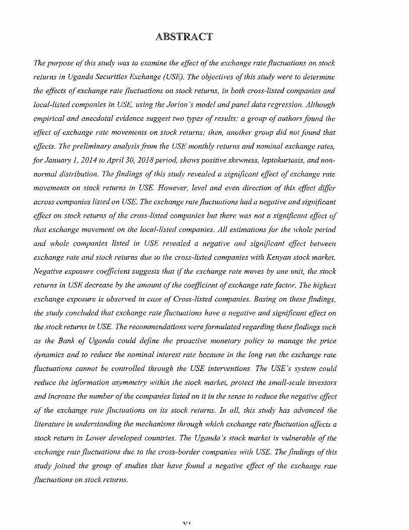
The purpose ofthis study was to examine the effect of the exchange rate fluctuations on stock
returns in Uganda Securities Exchange (USE). The objectives of this study were to determine
the effects of exchange rate fluctuations on stock returns, in both cross-listed companies and
local-listed companies in USE, using the Jorion ‘s model andpanel data regression. Although
empirical and anecdotal evidence suggest two types of results: a group ofauthors found the
effect of exchange rate movements on stock returns; then, another group did not found that
effects. The preliminary analysis from the USE monthly returns and nominal exchange rates,
for January 1, 2014 to April 30, 2018 period, shows positive skewness, leptokurtosis, and non-
normal distribution. The findings of this study revealed a significant effect of exchange rate
movements on stock returns in USE. Howevei~ level and even direction of this effect differ
across companies listed on USE. The exchange rate fluctuations had a negative and significant
effect on stock returns of the cross-listed companies but there was not a significant effect of
that exchange movement on the local-listed companies. All estimations for the whole period
and whole companies listed in USE revealed a negative and significant effect between
exchange rate and stock returns due to the cross-listed companies with Kenyan stock market.
Negative exposure coefficient suggests that if the exchange rate moves by one unit, the stock
returns in USE decrease by the amount of the coefficient ofexchange rate factor. The highest
exchange exposure is observed in case of Cross-listed companies. Basing on these findings,
the study concluded that exchange rate fluctuations have a negative and significant effect on
the stock returns in USE. The recommendations wereformulated regarding thesefindings such
as the Bank of Uganda could define the proactive monetary policy to manage the price
dynamics and to reduce the nominal interest rate because in the long run the exchange rate
fluctuations cannot be controlled through the USE interventions. The USE’s system could
reduce the information asymmetry within the stock market~, protect the small-scale investors
and increase the number of the companies listed on it in the sense to reduce the negative effect
of the exchange rate fluctuations on its stock returns. In all~ this study has advanced the
literature in understanding the mechanisms through which exchange rate fluctuation affects a
stock return in Lower developed countries. The Uganda ‘s stock market is vulnerable of the
exchange rate fluctuations due to the cross-border companies with USE. The findings of this
study joined the group of studies that have found a negative effect of the exchange rate
fluctuations on stock returns.
~7T
CHAPTER ONE
INTRODUCTION
i,O~ Introduction
Under this chapter, the background, problem statement, purpose, objectives, research
questions, hypotheses, scope, and significance of the study are presented in line with the
research title.
Li. Background to the study
1.1.1. Historical perspective
The interest for the connection between foreign exchange rate fluctuations and stock returns
goes back to the fall of the Bretton Woods system (1971-1972), known as Nixon Shock (Dufey,
1972 & Leeson, 2003). This system was replaced by a free-floating rates system in which the
price of currencies is determined by supply and demand of money (Abor, 2005).
The securities exchanges are probably the most vital parts of the present worldwide economy.
Nations around the globe rely upon securities exchanges for financial development regardless
of whether they are the generally new trend (Hur, 2018). In Europe, the year 1773 promoted
the adjustment in the market organization. As the volume of stocks increased, the requirement
for a sorted out commercial center to trade these stocks became important. Therefore, stock
merchants chose to meet at a London café, which they utilized as a market center. In the long
run, they assumed control over the café and changed its name to the “stock exchange.” Then,
the first exchange, the London Stock Exchange, was established, so it was constrained on the
grounds that organizations were not permitted to issue stocks until 1825 (Turner, Qing &
Walker, 2018).
In USA, the New York Securities Exchange (NYSE) was founded in 1817 because of the
restrictions of the London Stock Exchange (LSE). In this same period, the London Stock
Exchange was the fundamental Stock market in Europe and keeping in mind that NYSE was
the principal Stock market (Exchange) in America and the world (as today).

In 1971, the NASDAQ (National Association of Securities Dealers Automated Quotations
stock exchange) was founded to resolve some lacks of NYSE. The NASDAQ is the first
electronic stock exchange that allowed investors to buy and sell stock on a computerized,
speedily and transparent system without a need for a physical trading floor (Hom, 2012). In the
similar period, the former American’s president, Nixon took a unilateral decision to change the
fixed exchange rate to free-floating exchange rate and this last exchange rate regime was
adopted through the Jamaica Agreement on 1976 (Halm, 1977 & Irwin, 2013).
In Africa, the first securities exchange was founded in Egypt named Egyptian Exchange (EGX)
in 1883 followed by Casablanca Stock Exchange (CSE) in 1929. They adopted pegged-floating
exchange rate respectively. Today, there are 29 stock exchanges around Africa continent and
more than 2140 companies listed on them (Essays, 2013).
Today, numerous nations around the globe have their own particular market securities. Around
the world, many securities exchanges regularly rose in the nineteenth and twentieth centuries
not long after London Stock Exchange and New York Stok Exchange. The stock exchange
indices are additionally a critical part of present day securities exchanges. The Dow Jones
Industrial Average is apparently the most vital file in the word (DJIA) made by Wall Street
Journal editorial manager Charles Dow in 1885 (Thirunavukkarasu, 2006).
Exchange rate and the stock market price are interconnected. The world is transforming into a
village because of exchange liberalization and globalization. For example, foreign investors
are interested to put their capital in the securities exchanges worldwide. In this procedure,
global speculation is moving quickly and capital is moving over everywhere throughout the
world. The advantages of these financial specialists (Investors) are being controlled by the
foreign exchange. Also, insecurity in the exchange rate may realize vulnerability or generally
in these speculators. Then, the exchange rate is the vital determinant of securities exchange
fluctuations.
Uganda embraced the free-floating exchange rate system at the beginning of 1 990s which
implies the conversion of the Ugandan shilling versus the US dollar and other outside
currencies is dictated by demand and supply of cash (Onegi-Obel, 2016). The Uganda
Securities Exchange (USE) was created in 1997 as an organization limited by guarantee and
was licensed in 1998 by the Capital Markets Authority to work as an affirmed securities
exchange. A stock market is a focal place for exchanging of securities by authorized
dealers/brokers of firms, financial specialists, a delegate of speculators and an agent of issues.
It gives a credible platform for raising of capital; through the issuance of proper obligation,
equity and different instruments offered to the public. Along these lines, the Exchange gives
fundamental facilities to the private entity and government to fund-raise for business
development and empowers the public to own shares in companies listed on this stock market.
The first company quoted in USE was Uganda Clays Ltd (UCL) in 2000 and the first cross-
listed company with Nairobi Security Exchange was East Africa Breweries Ltd (EABL) in
2001 (Businge,.13 2014).
It is widely trusted that the exchange rate fluctuations are one of macroeconomic uncertainty
that ought to significantly affect the stock returns (Shapiro, 1975; Marston, 2001 and
Simakova, 2017). At that point, a firm has not a total control on exchange rate volatility and
the firm can go for administration of such hazard (Jorion, 1990).
1.1,2. Theoretical perspective
This study was focused on two theories related to exchange rate fluctuations and the stock
returns of a company listed at any stock exchange, which are: The Efficient Market Hypothesis
(EMH) and International Fisher Effect (IFE).
The Efficient Market Hypothesis implies that present stock prices completely reflect all
information accessible. This implies the value of the stock changes instantly when new
information is accessible. There are three levels of the EMH: Weak form, Semi-Strong form,
and Strong form efficiency (Fama, 1970).
One of the real ramifications of an efficient market is that, the present price changes instantly
as new information is accessible. For instance, assume that Intel was to declare they had
developed another approach to fabricate PC chips that would influence PCs to run ten times
quicker at a large portion of the price, yet that it would take no less than a year to execute in
the entirety of their assembling plants. An efficient market suggests that the stock price would
increment promptly when the information is accessible, not in 12 months’ time when the
innovation is executed or even later when additional benefits are gotten. Basically, the EMH
says that stocks react instantly to the Net Present Value (NPV) of new information (Harder,
2010).
However, the International Fisher Effect (IFE) was created at end of the Bretton Woods system
in 1971-1972, so the association between exchange rate and interest rate differentials appeared.

The International Fisher Effect (IFE) proposes that the exchange rate between two countries
should change vis-à-vis their nominal interest rates. The country which has a lower amount of
interest rate will see their currency be appreciated in the future spot exchange and country
which has a higher nominal interest rate, will see its currency be depreciated in the future spot
exchange (Buckley, 2004).
The International Fisher Effect (or Fisher’s open theory) is a speculation which deals with the
nominal interest rates between two counties in sense to determine the spot conversion
(exchange) of currencies (Eun & Resnick, 2011).
These economic theories have led this study especially the Efficient Market Hypothesis which
has been the main theory in this study.
1.1.3. Conceptual Perspective
The exchange rate fluctuation, the stock return and the return on market portfolio (market
index) are the key concepts in this study.
In finance, an exchange rate is a rate at which one currency will be traded for another with
respect to the market powers (the supply and the demand of a particular currency versus
another). In additionally viewed, it is as the estimation of one nation’s money in connection to
another money. The spot exchange rate is the present exchange rate; however, the forward
conversion (Exchange) rate refers to a swapping rate that is concluded and traded today
however for conveyance and payment on a particular future date. Something else, the
purchasing rate is the rate at which cash merchants will purchase foreign currency, and the
offering rate is the rate at which they will offer that currency (Abdulla, 2017). A currency is
appreciated whenever its demand is greater than the accessible supply and it will depreciate
whenever its demand is not as much as the accessible supply (Jorion, 1990). Central banks
ordinarily have little trouble to adjust the available money supply to suit changes in the demand
for cash because of business transactions (Speculations). It has been concluded that the
speculation can undermine the real financial development, specifically since the speculators
were able to forecast the future value of currencies and to take a profit on them. For transporter
organizations shipping products from one country to another, exchange rate fluctuations could
impact them severely.
However, the stock return is the money made or lost on a share or stock. The value of a stock
is calculated by a change in its prices such as its beginning price and its ending price. It’s
ensured that an investor sets and gets the best price when he wants to sell a specific stock. The
stock return, from the perspective of the stock exchange, measures the value of a specific
business, venture or company (Amihud, 2002).
On another hand, the return in market index is a weighted average of the specific stock returns
or other investment instruments from regarding a particular stock market, and it is computed
from the stocks’ prices of the selected stocks. Market indices show an entire stock exchange
situation and cash the market’s movements over a certain period. It is an instrument used by
stakeholders and investors to describe the stock exchange and to compare the return on specific
stock, investments (Arnott, Hsu & Moore, 2005).
Besides, the variables to consider in this specific study are: The Stock-Returns of the companies
listed on USE as dependent variable (DV5); also, the Exchange rate fluctuations (FX) [Uganda
shilling/Us dollar] and the return on market portfolio (Market index) [Uganda all share index]
as the independent variables (IVs).
1,1.4. Contextual Perspective
This study is related to the exchange rate fluctuation and stock returns in the context of
Ugandan Securities Exchange (USE).
The USE opened to exchange in January 1998 at that time, the exchange had just one listing, a
bond issued by the East African Development Bank and trading was limited on a handful
exchange a week (Onegi-Obel, 2016).
The USE took 16 years to undertake the fixed income instruments. It’s on July 2014 that USE
exchanged 16 firms (8 locally quoted companies and 8 cross-listed companies) and it had begun
the exchanging of fixed income instruments (for example treasury bond, preference share,
corporate bond, and debenture stock, also short-term financial instruments: commercial paper
and treasury bill). The USE works with the “African Stock Exchanges Association” (Baganzi,
Kim, & Shin, 2017).
The USE works in close relationship with the Dar es Salaam stock trade (Tanzania), the
Rwanda Stock Exchange, and the Nairobi Securities Exchange (Kenya). As indicated by
distributed reports in 2013. These Stock Markets could share their risks with the USE in the
short run and long run.
It’s in 20 July 2015 that the USE initiated its electronic trading platform, backed by three
independent data servers, cutting to three days (Muhumuza, 2015).
The USE possesses by 16 stockbrokers. In August 2016, a law was passed to enable the
shareholders to sell stocks to public members through initial public offering (Anyanzwa, 2016).
On 18 May 2017, the USE demutualized and enrolled as an “open organization, limited by
shares.” Then, the Companies quoted on it must have a minimum share capital ofUGX 1 billion
and net the net assets ofUGX 2 billion on the off chance that to keep on operating in this stock
trade (Oketch, 2017).
1,2. Problem statement
The foreign investments are increasing day by day in Uganda’s businesses; so, multi-national
and transnational corporations are playing increasingly important roles in Ugandan business.
Uganda is also engaging in a much wider range of cross-border transactions with different
countries and products. The companies have also been more active in raising financial
resources abroad. Every one of these improvements consolidates to give a boost to cross-
currency cash-flows and different countries. According to Tomanova (2016), when dealing in
foreign currencies, fluctuations in the exchange rates are bound to occur and this affects
positively or negatively the expected incomes of firms.
Uganda’s economy faces an issue due to exchange rate exposure. On 2015, the Bank of
Uganda’s governor, Mutebile, stated that: “Over the course of the 2014/15 fiscal year, the
Ugandan Shilling depreciated against the US dollar by 27 percent, by an estimated $700
million.” Uganda’s market has suffered during that period because export commodity prices
have fallen, demand in key export markets has weakened and it has become more difficult to
mobilize capital on international markets (Onegi-Obel, 2016).
In 2016, the ALSIUG dropped by 501 points which were 15% due to the influence of the cross
listed companies (Muhumuza, 2017).
However, information collected by Crested Capital Ltd demonstrates that USE’s aggregate
market turnover fell from Ush173.77 billion ($47.5 million) in 2016 to Ush96.17 billion ($26
million) in 2017, a gap of $21.5 million. There were critical outflows witnessed saw on key
companies such as Umeme Ltd with poor revenues, lower than the UshS million ($1,366)
posted in numerous trading sessions (The East Africa, 2018).
E
This implies that the stock’s values held by investors dropped significantly during these
periods. When a stock value (price) drops, it also impacts Uganda All-Share Index (ALSIUG),
which shows the changing average value of the stock values of all companies quoted on a stock
exchange, and which is utilized as a measure ofhow well a market is performing.
All those problems are due to the poor tools which can measure historically the factors which
affect Uganda’s business value and the poor tools to predict the future risk of devaluation of
the business in LDCs; also, there are few studies which have been done regarding the effect of
foreign exchange rate fluctuations on stock returns, especially regarding LDCs’ stock
exchange.
It is in this context that the current study is focused on the effect that the exchange rate
fluctuations can have on the stock returns in Uganda Securities Exchange.
1,3. Purpose of the study
The purpose of this research is to examine the effect of the exchange rate fluctuations on stock
returns in Uganda Securities Exchange (USE).
1.4. Objectives of the study
This study is guided by the following objectives:
1. To examine the effect of exchange rate fluctuations on stock returns of cross-listed
companies.
2. To examine the effect of the exchange rate fluctuations on stock returns of local-listed
companies in USE.
3. To examine the effect of the exchange rate fluctuations on stock returns of all companies
quoted in Uganda Securities Exchange (USE).
1.5. Research questions
This study sought to provide answers to the following questions:
Qi: Is there a significant effect of exchange rate fluctuations on stock returns of cross-listed
companies?
-7

Q2: Is there a significant effect of the exchange rate fluctuations on stock returns of local-listed
companies in USE?
Q3: Is there a significant effect of the exchange rate fluctuations on stock returns of all
companies listed in Uganda Securities Exchange (USE)?
1.6. Hypotheses
The following hypotheses have been tested in order to determine the effect between variables
considered in this study:
H0i: There is no significant effect of exchange rate fluctuations on stock returns of cross-listed
companies.
H02: There is no significant effect of the exchange rate fluctuations on stock returns of local
listed companies in USE.
H03: There is no significant effect of the exchange rate fluctuations on stock returns of all
companies listed in Uganda Securities Exchange (USE).
1,7, Scope of the study
Geographically, the study was carried out in Uganda precisely from USE (Uganda Securities
Exchange). Basing on the content, this study was limited to measure the effect of exchange rate
fluctuations on stock return’s in Uganda Securities Exchange during a sample period of 52
months (2014/01-2018/04).
Basing on the time period covered by this study, the data have been collected by considering a
long period and the researcher collected much of the recent data in order to obtain current
information on exchange rate fluctuations and stock return’s in Uganda Securities Exchange.
Besides, this provided an opportunity for further research in the excluded companies.
Theoretically, the study was anchored on the Efficient Market Hypothesis (EMH) and the
International Fisher Effect (IFE).
C)

1,8. Significance of the study
The results and findings of this study are beneficial to different stakeholders as they provided
a better understanding of the effect of exchange rate fluctuations on stock returns in Uganda
Securities Exchange.
Thus, this study aims to bridge the gap between the exchange rate fluctuation literature and the
studies on the stock market and determine whether there are actions over the stock returns
which could lead the negative effects of company’s reaction to exchange rate changes.
Exchange rate fluctuation is appropriated to money decisions which states that firms will
interpret the exchange rate fluctuation as a buffer against adverse cash flow shocks, particularly
if they have more opportunities for investment. This research will assist the stakeholders with
understanding the impact that the cross-listed companies can have on Uganda All Share
Exchange (ALSIUG).
This study is a great benefit to academicians and future researchers who will be undertaking
other researches related to it as it will be used as a reference. This is because it will contribute
to the body of knowledge on the association between exchange rate changes and stock returns.
Regarding the emergent stock market, the findings of this research has contributed to
improving the understanding of the effect of exchange rate fluctuations on the firms listed at
any emergent stock market. The recommendations which provided in this study will be of
benefit to the management of Uganda Securities Exchange and the companies listed on it
because they will point out the areas ignored in exchange rate changes and stock returns as well
as the ways of improving the quality of their analysis.

1.9. Operationalization of key terms
Exchange rate fluctuation is a fluctuation or variation of the trading rate regarding a specific
period (such as: day, week, month, quarter, etc.). Then, an exchange rate represents a
rate at which one currency will be traded for another by thinking about the worth of
each one respectively.
Stock return: A stock return is a difference between the price we have paid for it and its current
price (or actual price); a stock return can represent either positive, zero or negative
value. A stock can be a bond, a share, etc.
Stock market: Stock exchange or share market is the aggregate ofpurchasers and sellers (a free
system of financial exchanges, not a physical offices or discrete area) of stocks
(additionally called shares, bonds) which hold ownership guarantees on businesses;
these may incorporate securities quoted on a public stock exchange an also those
exclusive exchanged privately.
Market index: represent a price-weighted average of a certain type of stocks or other
instruments which measure stock’s value regarding a specific stock market.
CHAPTER TWO
LITERATURE REVIEW
2.0. Introduction
The present chapter reviews the literature related to the exchange rates, the stock returns and
stock market. It is subdivided into the theoretical review, conceptual review, empirical reviews
and research gaps. These points have been reviewed in line with the objectives of the study.
2.1. Theoretical review
This study was focused on two theories related to Exchange rates and the stock returns, which
are: The Efficient Market Hypothesis and the International Fisher Effect (IFE).
2.1.1. Efficient Market Hypothesis (EMil)
The EMH theory is all about the information related to the stock price and the volatility of its
price. The EMH is essential for the purpose of the current study because it permits to have a
look at the stock return and the speculations around it in the case to determine its price.
The efficient market hypothesis (EMH) stipulates that; the current stock’s price fully reflects
all information about its value. This means that the stock price changes immediately when new
information becomes available. In an efficient market, the price rapidly translates into the
available information. Then, it is difficult to “beat the market” (Fama, 1970).
The EMH theory suggests that the asset prices are determined by the demand and supply in the
competitive market with rational investors. Rational investors gather information very rapidly
and immediately incorporate this information into stock prices. Only new information, i.e.
news, cause a change in prices but the news, by definition, is unpredictable; therefore, a stock
market which is immediately influenced by the news is also unpredictable.
According to EMH theory neither technical (a study ofpast stock prices in an attempt to predict
future prices) nor fundamental analysis (financial analysis such as industry analysis, company
analysis, asset valuation etc.) can help the investor to select “under-valued stock”. Past price
contains no useful information and cannot predict the future change, today’s price is totally

independent from past price so it is waste of time to analyze past return and on the basis of
result attempt or expect to make a profit from a market.
Ifwe can take a look to the historical background of EMH theory, an efficient market is as old
as stock market itself but the hypothesis was first expressed by Louis Bachelier, a French
mathematician in 1900. In his dissertation, “The Theory ofspeculation”, he has suggested that
price fluctuations are random and do not follow any regular pattern.
Consider three hypothetical paths for price adjustments:
* Increase immediately to a new equilibrium level
* Increase gradually to the new equilibrium level
* First over-shoot and then settle back to a new equilibrium level
Figure 1: Pareto efficient
Source: Shafer and Hugo (1975). [Pareto efficiency or Pareto optimality is a state of allocation of resources from
which it is impossible to reallocate so as to make any one individual or preference criterion better off
without making at least one individual or preference criterion worse oft]. The Pareto efficient is used in
EMIT theory.
E
z
-2 0 2D.y .l.t*~2 —
The assumptions of EMH theory may be pointed out as follows (Akintoye, 2008):
~ In an efficient market, a stock price is always at the “fair” level, a stock price change
only when its fair value changes.
~- The market is efficient if the reaction ofmarket prices to new information is immediate
and unbiased.
> Stock prices immediately react on the news.
> Stock price changes are unpredictable because no one knows tomorrow’s news.
> Stock prices follow a random walk, if a price of today goes up nobody can tell what
would be the price of tomorrow.
> It is impossible for investors to consistently outperform in the market.
+ Forms of Efficient Market Hypothesis:
In 1970, Fama classified efficient market hypothesis in three categories according to
the level of information reflected in market prices: weak form, semi-strong form and
strong form; a summarized description of these different forms of market efficiency is
presented below:
V Weak-form
The weak form efficiency is also popularly known as ‘random-walk’. In a weak form ofmarket
efficiency stock prices reflect by all available trading information which can be derived from
the market data such as past price, trading volume, etc. So nobody can use information related
to past price to identify the undervalued security and make a big profit by them, it implies that
no one should be able to outperform the market using something that “everybody else knows”.
If the markets are efficient in weak form, technical trading rules cannot be used to make a profit
on a consistent basis (Emenike, 2017). This form ofmarket efficiency is called weak-efficiency
because the security prices are the most publicly and easily accessible pieces of information.
V Semi-Strong Form
In semi-strong form, all publicly available information is incorporated into current stock prices.
Publicly available information includes past price information plus company’s annual reports
(such as financial reports, balance sheet and profit and loss account), company’s announcement,
macroeconomic factors such as (unemployment, etc.) and others. Some information (to the
extent anticipated in advance) is discounted even before the event is announced and some
before the event took place. Such matters as earnings reports, bonus, and rights affect the
market even in anticipation before the formal announcements. Semi-strong form implied that
share prices adjust to publicly available new information very rapidly and in an unbiased
fashion, such that no one should be able to outperform the market using something that
“everybody else knows”.
V Strong Form
In a strong form of efficiency stock prices quickly reflect all types of information which include
public information plus companies inside or private information. Thus, it is the combination of
public and private information that is incorporated into current prices. This form implies that
even companies’ management cannot make a profit from inside information; they cannot take
advantage of inside affairs or important decision or strategies to beat the market. According to
strong-form market efficiency, inside information is also already incorporated into stock prices,
the common rationale behind this is unbiased market anticipation that already reacts into a
market before companies’ strategic decision. A strong form of efficiency is hard to believe in
practice except where rules and regulations of law are fully ignored (Reilly & Brown, 2008).
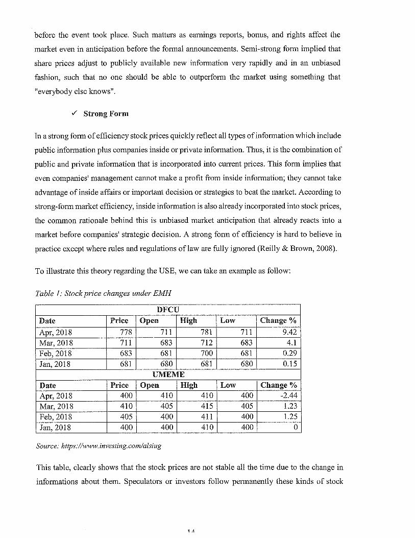
To illustrate this theory regarding the USE, we can take an example as follow:
Table 1: Stockprice changes under EMH
_____ DFCUDate Price Open High Low Change %Apr, 2018 778 711 781 711 9.42Mar, 2018 711 683 712 683 4.1Feb, 2018 683 681 700 681 0.29Jan, 2018 681 680 681 680 0.15
UMEMEDate Price Open High Low Change %Apr, 2018 400 410 410 400 -2.44Mar, 2018 410 405 415 405 1.23Feb, 2018 405 400 411 400 1.25Jan, 2018 400 400 410 400 0
Source: https://www. investing. com/alsiug
This table, clearly shows that the stock prices are not stable all the time due to the change in
informations about them. Speculators or investors follow permanently these kinds of stock
1,1
prices indices in the purpose to determine a type of stock which can be more profitable in
future.
The stock returns changes are essential factors in the current study when it comes the time to
establish the influence that the exchange rate fluctuations can have on then by considering a
certain period.
2,1.2. International Fisher Effect (IFE)
The IFE is also an important theory related to this study because it permits to know how the
spot exchange rate between two nations is determined by considering their different currencies.
Exchange rate incorporates some microeconomic information which cannot be ignored when
it comes the time to evaluate the stock market. The spot exchange rate or real exchange rate
shows how a particular nation’s currency is performing during a period of time (Shapiro, 2013).
Historically, the International Fisher Effect theory (IFE) was developed at the end of the
Bretton Woods agreement (1971-1972), so the association between exchange rate and interest
rate differentials appeared. The IFE theory suggests that the exchange rate between two
countries should change by a sum similar to the difference between their nominal interest rates.
If the nominal rate in one country is lower than another, the currency of the country with the
lower nominal rate should appreciate against the higher rate country by the similar sum
(Hatemi-J & Irandoust, 2008).
The IFE (or Fisher’s open hypothesis) recommends that the differences in nominal interest rates
between two nations equal the expected changes in the spot exchange rates of these nations at
a specific time. The connection between interest rate and inflation first set forward by Fisher
(1930), proposes that the nominal interest rate in any period is equal to the sum of the real
interest rate and the expected rate of inflation. This is termed the Fisher Effect. He hypothesized
that the nominal interest rate could be decomposed into two components, a real rate plus an
expected inflation rate [(1 +i) = (1 +r)( 1 +Inflation Rate), Where i= nominal interest rate and r =
real interest ratel (Hetemi-J & frandoust, 2008)
International Fisher Effect says, in other words, the percentage change in the spot exchange
rate over time is governed by the difference between the nominal interest rates of two
currencies.
Mathematically, International Fischer effect is expressed as follow (Hetemi-J, 2009; Cheol &
Resnick, 201 1):
SpOt today SP0tAfterayear ‘USA — ‘Uganda (1)
Spot After a year 1 + i Uganda
For example, suppose in January 2018, the nominal interest rate in Uganda is 12% per annum
and it is 8% in the USA, then UGX is expected to depreciate vis-a-vis USD. Plugging the
interest rate on the right-hand side of, we get:
IUSAIUganda8%12%
+IUgaflcla — 0
Hence, the percentage difference between the spot rate prevailing today and spot rate to prevail
after a year should be equal to -3.57%. This indicates that UGX will depreciate by 3.57% at
the end of one year, i.e.; 1st January 2019.
In other words:
UGX/USD — Spot Aftera year = —3.57% (3)
Spot After a year
According to the same example, the USD appreciation, amount, is governed by:
5’POttoctay — Spot After a year = ~ Uganda — USA (4)
SPOt Afterayear 1 + 1USA
~UgancLa — ‘USA 12% —8%= 3.7/o(5
l+LUSA 1+8%
In other words, USD is expected to appreciate by 3.7%.
The percentage of appreciation or of depreciation is governed by nominal interest rate
differential according to this theory.
These economic theories, which are based on assumptions and perfect situations, help to
illustrate the basic fundamentals of stock returns (prices) and the exchange rates.
2.2, Conceptual Review
For the past years, scientists have been experimentally researching on the exchange rate
fluctuations and the stock returns. Therefore, the exchange rate fluctuation is acquired from a
regression of stock returns on an exchange rate changes, regularly with extra control variables
such as market index. Then, firms must be computed by some convergence characteristics to
reduce errors and bias (Bodnar & Gentry, 1993; Jorion, 1990). Several numbers of studies done
on exchange fluctuations and stock returns, typically use a month horizon for measuring returns
(Simakova, 2017).
Exchange rate variability is one of the macroeconomic sources of vulnerability which has
influencing firms exposed to open economy. Exchange rate fluctuation impacts the working
cash flows and business value through the transactions. In addition, outside shocks may make
an interdependence between exchange rate variabilities and stock returns. Therefore, it
becomes critical to expect an association between exchange rate variabilities and stock returns
(Prasad & Rajan, 1995).
This section reviews the key concepts regarding this thesis’ title such as exchange rate
fluctuation, stock return and stock market (IV and DV).
2.2.1. Exchange rate, exchange rate fluctuation and exchange rate regime
This point summarizes the concepts concerning the exchange rate, exchange rate fluctuation
and exchange rate regime.
2.2.1.1. Exchange rate
In finance, Then, an exchange rate represents a rate at which one currency will be traded for
another by thinking about the worth of each one respectively.
Economists define a real exchange rate as a purchasing power that one currency can have
versus another currency at spot exchange rates. It represents units’ number of one country’s
currency needed to buy a certain number of goods in the other country’s currency in the foreign
exchange market (Reinhart & Rogoff, 2004).
In the same way, we can take an example of an interbank exchange rate of 3,700 Uganda
shillings (UGX) which equals to $1 United States dollar; it means that UGX 3,700 will be
traded for each US $1 or this US $1 will be traded for each UGX 3,700. In this case, it is said
that the price of a dollar in relation to Uganda Shillings, or equivalently that the price of a UGX
in relation to dollars is $1/3,700. Then, we can take a look at the following example of an
exchange rate:
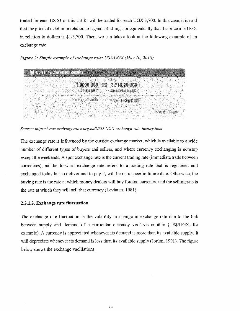
Figure 2: Simple example ofexchange rate: US$/UGX (May 10, 2018)
U
Source: https://www. exchangerates. org. uk/USD- UGX-exchange-rate-history.htrnl
The exchange rate is influenced by the outside exchange market, which is available to a wide
number of different types of buyers and sellers, and where currency exchanging is nonstop
except the weekends. A spot exchange rate is the current trading rate (immediate trade between
currencies), so the forward exchange rate refers to a trading rate that is registered and
exchanged today but to deliver and to pay it, will be on a specific future date. Otherwise, the
buying rate is the rate at which money dealers will buy foreign currency, and the selling rate is
the rate at which they will sell that currency (Leviatan, 1981).
2.2.1.2. Exchange rate fluctuation
The exchange rate fluctuation is the volatility or change in exchange rate due to the link
between supply and demand of a particular currency vis-à-vis another (US$/UGX, for
example). A currency is appreciated whenever its demand is more than its available supply. It
will depreciate whenever its demand is less than its available supply (Jorion, 1991). The figure
below shows the exchange vacillations:
In
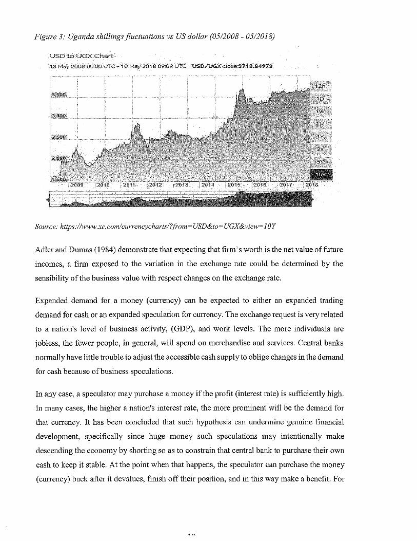
Figure 3: Uganda shillings fluctuations vs US dollar (05/2008 - 05/2018)
USD to UGX Chart
13 May 2008 0000 UTC -10 May2018 09~09 UTC USDfUGX cLose371 3~84972
3~500
2015 2016 2017 2Ô18
Adler and Dumas (1984) demonstrate that expecting that firm’s worth is the net value of future
incomes, a firm exposed to the variation in the exchange rate could be determined by the
sensibility of the business value with respect changes on the exchange rate.
Expanded demand for a money (currency) can be expected to either an expanded trading
demand for cash or an expanded speculation for currency. The exchange request is very related
to a nation’s level of business activity, (GDP), and work levels. The more individuals are
jobless, the fewer people, in general, will spend on merchandise and services. Central banks
normally have little trouble to adjust the accessible cash supply to oblige changes in the demand
for cash because of business speculations.
In any case, a speculator may purchase a money if the profit (interest rate) is sufficiently high.
In many cases, the higher a nation’s interest rate, the more prominent will be the demand for
that currency. It has been concluded that such hypothesis can undermine genuine financial
development, specifically since huge money such speculations may intentionally make
descending the economy by shorting so as to constrain that central bank to purchase their own
cash to keep it stable. At the point when that happens, the speculator can purchase the money
(currency) back after it devalues, finish off their position, and in this way make a benefit. For
3~O0O
2~6OG
2009 2010 2011 2012 2013 2014
Source: https://www.xe. com/currencycharts/?frorn USD&to’ UGX&viewl OY

carrier firms shipping products from one country the onto another, exchange rate volatility can
impact them severely.
2.2.1.3. Exchange rate regime
After the Bretton Woods system (1970-1972), every nation decides about which type exchange
rate that it will apply to its currency. There are three kinds of exchange rate: the free-float,
pegged float and fixed regime (O’Connell, 1968, & Nakamura & Steinsson, 2018).
The free-floating exchange rate is defined when the spot exchange rate is controlled by the
market powers such as supply and demand of this specific currency. The exchange rate for such
regime is probably going to change constantly as is quoted on monetary markets around the
globe.
A changeable (adjustable) peg float system is a regime of fixed exchange rate, but with a
provision for the revaluation (usually devaluation) of a currency. For example, in the period of
1994 and 2005, the Chinese yuan renminbi (RMB) was pegged to the United States dollar at
RMB 8.2768 to $1. China was by all account not the only nation to do this; from the finish of
the world war 2 until 1967, Western European nations all kept up the fixed exchange rates
regime with the US dollar based on the Britton Woods system. But that system had been
surrendered to give place to a free-floating exchange rate due to market speculations. The
former President Richard M. Nixon in his speech in August 15th, 1971, put a break to the fixed
exchange rate regime which is known as Nixon shock (Lehrman, 2011).
Uganda adopted the free-floating regime at the beginning of the 1 990s (Caramazza & Aziz,
1998).
2.2.2. Stok Return
A return (financial return) is a cash made or lost on an investment or a speculation. A return
can be expressed as the variation in dollar value of a share or an investment after a period of
time. A return can be expressed as a rate got from the proportion ofprofit to investment (Dichev
& Piotroski, 2001).
A stock return is a difference between the price we have paid for it and its current price (or
actual price); a stock return can be positive, zero or negative, negative. The adjustment in an
estimation of a specific stock (Bond, offer or value) might be because of various financial
viewpoints, such as interest rate, GDP, exchange rate, and so on. The stock price is a very
A
important parameter to evaluate a stock or a firm (in case of securities market) by stakeholders
to ensure that they will get the best price when they need to offer a stock or a business. The
stock return can be calculated as taking after:
Ending price—Starting priceStock Return = * 100 (in percentage)
Starting price
Source: www.fool. corn/knowledge-center/return-stock-mark. aspx
As indicated by Shapiro (1975), theoretical ideas he developed, propose that a multinational
firm with export sales and in competition should show exchange rate fluctuation and that the
company’s exposure should be related through the proportion of export sales, the level of
substitutability between local and imported factors of production and the degree of
competitions.
2.2.3. Stock market return and Market index (Return on market portfolio)
+ Stock market return
The securities exchange returns are the profits that the stakeholders create out of the share
trading system. This return could be a benefit through exchanging or in kind ofdividends given
by the enterprise to its shareholders every once in a while. The stock exchange returns can be
also referred through dividends announced by the companies (Ang, et aL, 2006).
Toward the finish of each quarter, a firm making benefit offers a piece of the kitty to the
investors. This is one of the benefits of securities exchange return on which shareholders could
anticipate. The most well-known type of generating a securities exchange return is to exchange
in through the secondary market (Market of second hand’s stock). In the secondary market, a
shareholder could gain a securities exchange return by purchasing a stock at a lower price and
selling at a higher price. Securities exchange returns are not fixed guaranteed returns and are
concerned with market risks. They can be certain or negative. Securities exchange returns are
not homogeneous and may change from financial specialist to speculator depending upon the
measure of hazard which one is set up to take and the nature of his stock market analysis.
Contrary to the fixed incomes generated by the bonds, the securities market returns are variable
in nature. The thought behind the stock return is to purchase cheap and sell dear. Therefore, a
risk is an integrated part of this market and a speculator can likewise observe a negative return
in case ofwrong speculations. A financial specialist speculates on the basis of fundamental and
technical analyses. Fundamental Analysis examines relevant information (return on assets,
history of profits, cash flow) related to the business, which could affect the intrinsic of the
stock. This investigation helps in anticipating the price change of the stock based on its
fundamental strength. Fundamental analysis is generally relevant for the long-term (Maurya,.
2016 & Economywatch, 2018).
+ Market index
A stock market index or securities market index is an estimation of a section of the stocks or
the stock market. It is calculated from the prices of selected securities (typically a weighted
average). It is an instrument utilized by stakeholders and financial specialists to depict the
market and to look at the return on particular investments (Market index, 2018).
Market indexes are intended to represent an entire stock market and track the market’s changes
over time (Chordia at al., 2014).
Index values enable financial specialists to track changes in market prices over short run or
long period. For example, Uganda all share index (ALSIUG) is examined by combining 16
types of stock prices regarding companies listed in USE, shareholders can track changes in the
indexes’ values over time and use it as a monitoring for their particular portfolio returns.
In the event that an index goes up for one level or 1%, this implies a gathering of stocks has,
correspondingly, augmented its value by one level also and become more attractive to
investors.
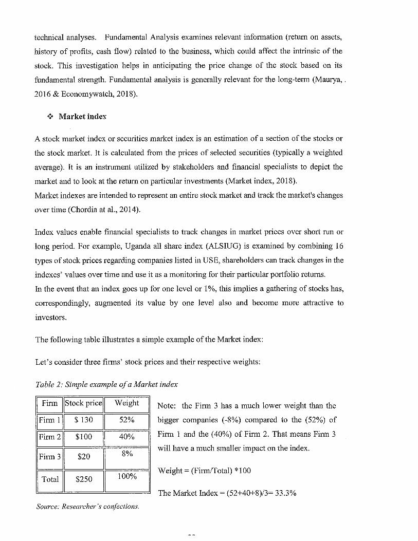
The following table illustrates a simple example of the Market index:
Let’s consider three firms’ stock prices and their respective weights:
Table 2: Simple example ofa Market index
Firm ~Stock price~ Weight
Firm 1 $130 52%
Firm2 $100 40%
Firm3 $20 8%
Total $250 100%
Note: the Firm 3 has a much lower weight than the
bigger companies (-8%) compared to the (52%) of
Firm 1 and the (40%) of Firm 2. That means Firm 3
will have a much smaller impact on the index.
Weight = (Firm/Total) * 100
The Market Index = (52+40+8)13= 33.3%
Source: Researcher’s confections.
2.3. Empirical review
A certain number of empirical studies have been conducted in exchange rate fluctuations and
stock returns in developed, emerging and Lower developed countries (LDCs).
The first empirical studies, which started in developed market, such as in U.S. markets, include
the empirical studies the effect of the foreign exchange rate fluctuations on U.S. firms (for
example, Shapiro, 1975, Jorion, 1990, Bodnar, & Gentry 1993, Choi & Prasard, 1995); these
studies, typically found low or negligible levels of exposure for most firms regarding the
exchange fluctuations, even when the firms examined have significant foreign operations
(Bodnar & Marston, 2002). Then, Choi and Prasad (1995) examined exchange risk sensitivity
and its determinants: A firm and industry analysis of U.S. multinationals. They developed a
model of firm valuation (Rat = ctj-+ f3j Rt + yjet+ V~t) to examine the exchange risk sensitivity of
409 U.S. multinational firms during the sample period of llyears (1978-1989). Their results
stipulated that approximately 60% of the firms were benefited when the dollar was depreciated
instead of 40% lost during the same period (of their study). They found also that the variation
in exchange risk sensitivity of individual firms is related to firm-specific operational variables
such as sales, assets, and profits, and its exchange risk sensitivity. It means that there was a
positive relationship between exchange rate fluctuations and the firm valuation.
In Europe, Simakova (2017) conducted a study on the Impact of Exchange Rate Movements
on Firm Value in Czech, Hungary, Poland, and Slovakia. The aim of her paper was to evaluate
the effect of exchange rates on the value of companies listed on stock exchanges in these
countries. Her Paper applies Jorion!s (1990) two factor model (Rit= th + ~3iRMt + öiRFXt + ~i;
where: c~i is the constant term, Rit, is the stock return of firm i over time period t, RMt is the
return on the market index, J]~ is the firm’s market beta and RFX t is the real effective exchange
rate. Hence, the coefficient & reflects the change in returns that can be explained by movements
in the exchange rate after recognition on the market return) and panel data regression for the
sample period of l4years (2002-20 16). All-time series she used for estimating the exchange
rate exposure on the firm value were on a monthly frequency. Therefore, her findings revealed
a negative relationship between exchange rate and value of stock companies. She estimated
that all tested markets seem to be exposed to the exchange rate risk, at least, at 10 %
significance level during the sample period.

In the same area, Tomanova (2016) conducted a study on exchange rate volatility exposure on
corporate cash flows and Stock Prices: The Case of Poland. Her paper analyzed the foreign
exchange rate exposure on the value of publicly listed companies in Poland on the basis of
stock prices and more than 6,000 large, medium-sized and small firms on basis of corporate
cash flows. Her analysis covered a sample period of from llyears (2003 to 2012 to 2014). In
the case of stock prices, she used a panel regression by using monthly data. Her results showed
that a significant number of these firms, especially small and medium-sized is exposed.
It is well known that the emerging stock markets are riskier than the developed stock markets;
therefore, in its study, Flota (2014) examined the impact of exchange rate movements on firm
value in emerging markets: The Case of Mexico. Using a sample of non-financial firms from
Mexico Stock Exchange (BMV), she collected data from a sample period between the first
quarter in 1994 to the third quarter in 2003. She used a two-stage model, based on the empirical
form of the CAPM (Capital Asset Pricing Model) {R~~ a1 + /3~ RM~ + & FXt + si~}. However,
her findings suggested that the firms which have heavily activities on international sales are
significantly less sensitive to exchange rate movements than firms that rely primarily on
domestic sales. He found a positive relationship between the exchange rate exposure and the
firm valuation.
Thirunavukkarasu (2006) hypothesized that the exchange rate exposure of the EMNCs would
be greater than the developed market multinationals (DMNCs). Using a sample of 212 MNCs
from emerging and developed markets, he found that: More than 60% of the EMNCs and the
DMNCs are significantly exposed to exchange rate fluctuations. Then, by analyzing the
magnitude of the exposure of that sample, he found that EMNCs are 20% more exposed than
developed market DIv[NCs.
In another hand, Yaw-Yih (2004) had examined the Fluctuations of Exchange Rate on the
Valuation of Multinational Corporations as Taiwan’s Samples. Considering a sample (Panel)
of 11 years (from 1991 to 2002), he found that the Exchange rate fluctuations affected stock
returns significantly in all industries.
In Africa, a certain number of empirical studies was done regarding the exchange rates
exposure on the firm valuation. It’s the case of Mugera (2013) who investigated on “The effect
of foreign exchange risk management on firm value of Firms listed at Nairobi Securities
Exchange (NSE)”. He found that foreign exchange risk (rate) does not significantly affect the
firm value.
Mwangi (2013) tried to analyze “The effect of foreign exchange risk management on financial
performance of microfinance institutions in Kenya”. He analyzed the data collected on 44
MFI’s registered by the Association of Microfinance Institutions of Kenya and he found out
that a strong positive relationship exists between financial performance of these institutions
and the foreign exchange rate.
Mbubi (2013) tried to analyze the effect of foreign exchange rates on the financial performance
of listed firms at the Nairobi Securities Exchange. He had used a linear regression to analyze
the data which he had collected among 41 firms listed at Nairobi Securities Exchange during a
period of 10 years (2002-2012). From the findings of his study, he found that listed firm’s
financial performance is negatively affected by the foreign exchange rates movements.
In Uganda, some studies were conducted on Ugandan Securities exchange and Uganda’s
exchange rate fluctuations such as the work of Emenike and Kirabo (2018) and Nampeera
(2015), Oluka (2010), among many others. Emenike and Kirabo (2018) sought to evaluate the
Ugandan Securities Exchange (USE) for evidence of a weak-form efficient market hypothesis
in the context of random walk model by using both linear and non-linear models. Their
preliminary analysis from the USE daily returns, for the September 1, 2011 to December 31,
2016 period, showed negative skewness, leptokurtosis, and non-normal distribution. They used
the linear and non-linear models to estimate the weak form efficient of the USE. They found
the weak form efficient in both models regarding this specific stock market. Their study
concluded that USE returns may only be predicted using non-linear models and fundamental
analysis. In other words, linear models and technical analyses may be clueless for predicting
future returns.
Nampeera (2015) examined the “Foreign Exchange risk management and performance of forex
bureaus in Uganda”. His study focused on a sample size of 177 forex bureaus out of a
population size of 264 in Kampala city Centre; using a primary data, he found that forex
bureaus have experienced positive and unstable performance over the period and also firm have
implemented numerous foreign exchange risk management practices to assess and lessen the
impact of risk losses due foreign exchange fluctuations.
Oluka (2010) sought to examine the relationship between firm characteristics, foreign
exchange risk management practices and the performance of Ugandan export firms.
Using a cross-sectional and correlation research designs, he found that there is no significant
relationship between firm characteristics, foreign exchange risk management practices and the
performance of Ugandan export firms.
2,4. Research Gaps
This study is emphasizing the effect of exchange rate fluctuations on stock returns in Uganda
Securities Exchange (USE) which are a particular case regarding the theoretical and empirical
findings.
Several studies related to the relationship between exchange rate fluctuations (Exposure) and
the stock returns (firm values) were done on a certain number of countries such as US, Mexico,
Brazil, Kenya, Ghana, Czech, Poland, etc.; then researchers did not have the same conclusions
about the puzzle that concerns the exchange fluctuations. That is the reason why Bodnar and
Marston (2002) tried to elaborate the Simple Model theory which can be applied in term of
Exchange rate exposure but their model is not actually the only reference model when it’s come
the time to measure the effect of the foreign exchange rate fluctuations on stock returns. This
is due to the particularity of each country vis-à-vis another county. Every country has his
specific economic situation. The relationship between exchange rates and stock returns is too
recent because the theories related to it, have been developed after the fall of Bretton Woods
system (Shapiro, 1975, Jorion, 1990, & Choi & Prasad, 1995).
The macroeconomic aggregates of Uganda are different from others country by considering
the inflation rate, interest rate, a rate of unemployment, GDP, monetary policy, the period in
which the study have been done, etc.
Then, the gap between the current research and others is related to the macroeconomic
aggregates of Uganda [to firm valuation (size, sales, profit, etc.)] and there is, also, a lack of
studies related to this particular subject under study in Uganda area. This study will help also
Uganda’s investors and shareholders at USE to take into consideration the influences that the
cross-listed companies can have on their stock or share returns.

CHAPTER THREE
METHODOLOGY
3.0. Introduction
Six sections have constituted the frame of this chapter, such as research design, data collection,
sample period, model specification, measurement of variables and data analysis have been
presented.
3.1. Research design
This study has used a quantitative approach with an ex-post-facto research design. Indeed,
employing the experimental method in research is sometimes impractical or prohibitively
costly in time, money, and effort; in other instances, it is unethical or immoral. Ex post facto
research is ideal for conducting social research when is not possible or acceptable to manipulate
the characteristics of human participants. It is a substitute for the experimental research and
can be used to test hypotheses about cause-and-effect or correlational relationships, where it is
not practical or ethical to apply a true experimental even a quasi-experimental design (Neil,
2010).
For example, explain a consequence based on antecedent conditions; determine the influence
of a variable on another variable, etc. Ex post facto research uses data already collected, but
not necessarily amassed for research purposes (Cohen, Manion & Morison, 2000).
3,2. Nature of source of Data
The current study has used the secondary data only. The data had been collected regarding all
companies listed at Uganda Securities Exchange (USE); the USE currently has 16 listed
companies comprising of 8 local listed companies and eight cross-listed firms (Appendix I).
The data have been collected via different sources such as: the annual reports of different listed
companies at Uganda Securities Exchange (USE), the Bank ofUganda (bou.or.ug), the Uganda
Securities Exchange (use.or.ug) and Investing.com
Then, the data for the exchange rate exposure have been collected through Bank of Uganda;
however, the data concerning the stock returns and market indices have been found via annual
reports of listed companies at USE, USE, and Investing.com
3.3. Sample period
This study used the quantitative data which have been collected between 2014/01 and 2018/04
which are 52 months. The choice of this period is related to the situation in which the USE had
registered 16 companies on its stock exchange in 2013. This current study concerns 16 listed
companies and the data collected, have been related to these companies. The purpose of this
specific sample period is to cash all sensibilities or informations about these firms during that
sample period.
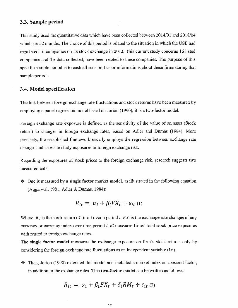
3.4. Model specification
The link between foreign exchange rate fluctuations and stock returns have been measured by
employing a panel regression model based on Jorion (1990); it is a two-factor model.
Foreign exchange rate exposure is defined as the sensitivity of the value of an asset (Stock
return) to changes in foreign exchange rates, based on Adler and Dumas (1984). More
precisely, the established framework usually employs the regression between exchange rate
changes and assets to study exposures to foreign exchange risk.
Regarding the exposures of stock prices to the foreign exchange risk, research suggests two
measurements:
+ One is measured by a single factor market model, as illustrated in the following equation
(Aggarwal, 1981; Adler & Dumas, 1984):
~ = c~ + f3~FX~ + 6jt (1)
Where, R~1 is the stock return of firm I over a period t, FX~ is the exchange rate changes of any
currency or currency index over time period t, /31 measures firms’ total stock price exposures
with regard to foreign exchange rates.
The single factor model measures the exchange exposure on firm’s stock returns only by
considering the foreign exchange rate fluctuations as an independent variable (IV).
+ Then, Jorion (1990) extended this model and included a market index as a second factor,
in addition to the exchange rates. This two-factor model can be written as follows.
R1~ = a1 + ,81FX~ + 6~RM~ + Ett (2)
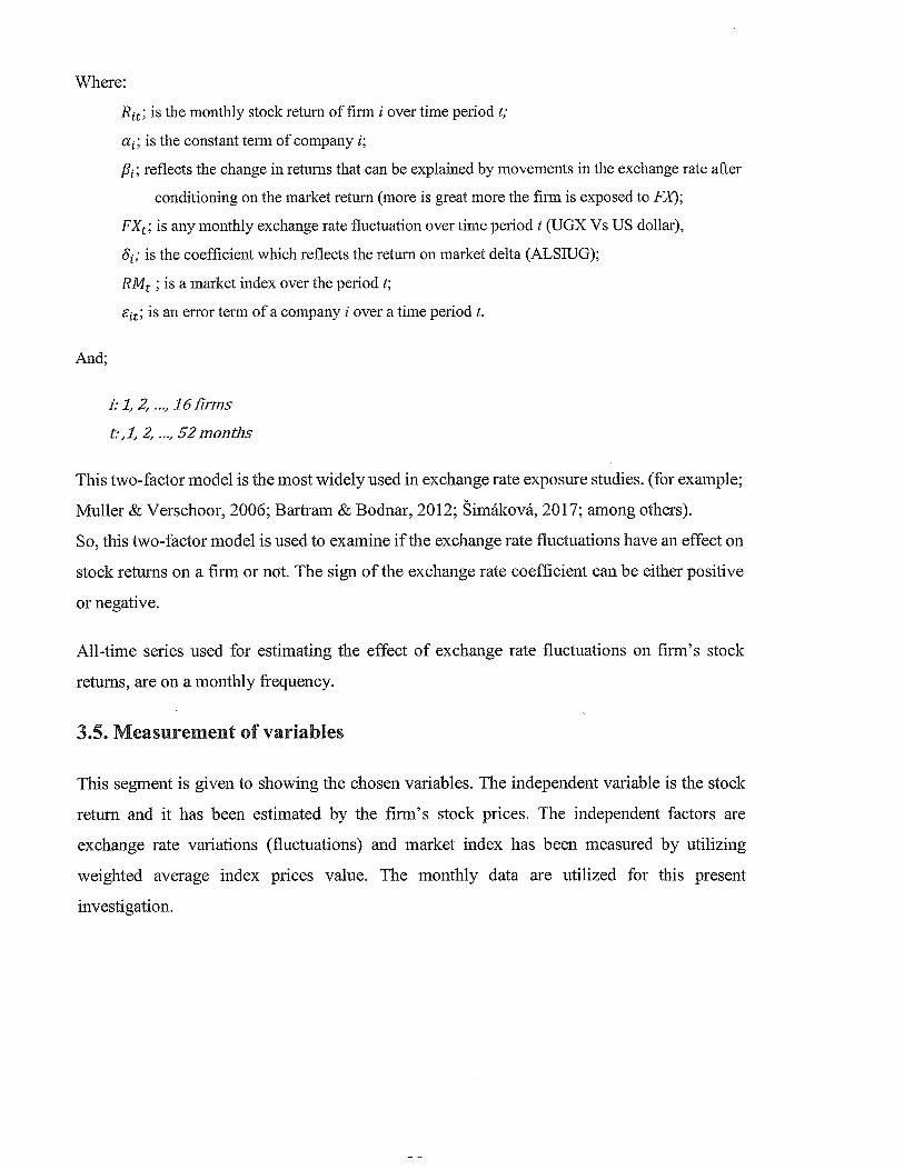
Where:
R1~; is the monthly stock return of firm i over time period t;
a~; is the constant term of company i;
f?~; reflects the change in returns that can be explained by movements in the exchange rate after
conditioning on the market return (more is great more the finn is exposed to FX);
FX~; is any monthly exchange rate fluctuation over time period t (UGX Vs US dollar),
6~; is the coefficient which reflects the return on market delta (ALSIUG);
RM~ ; is a market index over the period t;
~; is an error term of a company i over a time period t.
And;
1: 1,2, ...,l6firms
t:,1,2,...,S2months
This two-factor model is the most widely used in exchange rate exposure studies. (for example;
Muller & Verschoor, 2006; Bartram & Bodnar, 2012; ~imáková, 2017; among others).
So, this two-factor model is used to examine if the exchange rate fluctuations have an effect on
stock returns on a firm or not. The sign of the exchange rate coefficient can be either positive
or negative.
All-time series used for estimating the effect of exchange rate fluctuations on firm’s stock
returns, are on a monthly frequency.
3.5. Measurement of variables
This segment is given to showing the chosen variables. The independent variable is the stock
return and it has been estimated by the firm’s stock prices. The independent factors are
exchange rate variations (fluctuations) and market index has been measured by utilizing
weighted average index prices value. The monthly data are utilized for this present
investigation.
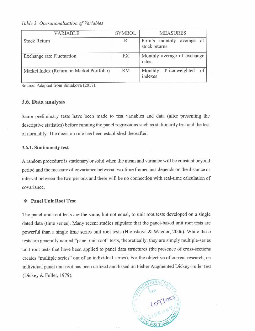
Table 3: Operationalization of Variables
VARIABLE SYMBOL MEASURES
Stock Return R Firm’s monthly average ofstock returns
Exchange rate Fluctuation FX Monthly average of exchangerates
Market Index (Return on Market Portfolio) RM Monthly Price-weighted ofindexes
Source: Adapted from Simakova (2017).
3.6. Data analysis
Same preliminary tests have been made to test variables and data (after presenting the
descriptive statistics) before running the panel regressions such as stationarity test and the test
of normality. The decision rule has been established thereafter.
3.6.1. Stationarity test
A random procedure is stationary or solid when the mean and variance will be constant beyond
period and the measure of covariance between two-time frames just depends on the distance or
interval between the two periods and there will be no connection with real-time calculation of
covariance.
•• Panel Unit Root Test
The panel unit root tests are the same, but not equal, to unit root tests developed on a single
dated data (time series). Many recent studies stipulate that the panel-based unit root tests are
powerful than a single time series unit root tests (Hlouskova & Wagner, 2006). While these
tests are generally named “panel unit root” tests, theoretically, they are simply multiple-series
unit root tests that have been applied to panel data structures (the presence of cross-sections
creates “multiple series” out of an individual series). For the objective of current research, an
individual panel unit root has been utilized and based on Fisher Augmented Dickey-Fuller test
(Dickey & Fuller, 1979).

Fisher — ADF
The method chose to deal with panel unit root regressions (tests), utilizes Fisher’s (1932) results
to determine the tests that join the p-values from individual unit root analyses. This thought
had been implemented by two researchers such as Maddala and Wu (1999), and Choi (2001).
The Fisher-ADF and Fisher-PP tests all permit for single unit root procedures so thatp
values may change through cross-sections. The panel stationarity tests are all identified by the
combining of individual unit root tests to determine a particular panel result.
The below table point out the basic characteristics of the panel unit root analyses available in
EViews related to Fisher-ADF and Fisher-PP:
Table 4: Panel Unit Root Testing
TEST NULL ALTERNATIVE
Fisher-ADF Unit Root Some Cross-sections without Unit Root
Fisher-PP Unit Root Some Cross-sections without Unit Root
Source: http://www.eviews.comlhelp/helpintro.html#page/contentladvtimeser-Panel_Unit_Rootjesting.html
The probability’s value which has been utilized to reject the null hypothesis must be less than
5% (p-value < 0.05). We tested each series of stock returns, exchange rate volatilities and
returns on market portfolio one by one for all listed companies in USE.
3.6.2. Panel Regression
The regression analysis looks to discover the connection between one or more independent
factors (variables) and a dependent variable.
The ordinary least squares (OLS) are one of the popular approaches regarding the regression
process estimators which are highly sensitive to (i.e. not robust regression against) outliers’
residues or errors. The gap found among the data anticipated by the regression (formula) and
the observed information is called residual. The outliers are the type of data distributions which
do not follow the path of the other data distributions. Only one bad data point or outlier can
make regression results meaningless (Mack, 2016).
However, the robust regression represents a type of regression approach designed to
overcome limitations due to the traditional Ordinal Least Squares regression’s methods
(Chatterjee & Mächler, 1995).
+ Robust Regression (Robust Least Squares methods)
The OLS have positive properties if their assumptions are verified (such as: The linear in
parameters among the model specification, mean should be equal to zero, normal distribution
residual, perfect collinearity, etc.), but can give misleading results if those assumptions are not
verified; thus OLS are not robust to violations of its assumptions. The Robust regression refers
to a variety of regression techniques established to be robust, or less sensitive to outliers or
error terms. EViews offers three distinct techniques of analysis related to the robust regression
such as M-estimation (Huber, 1973), S-estimation (Rousseeuw & Yohai, 1984), and MM-
estimation (Yohai, 1987).
The three methods differ in their emphases:
o M-estimation addresses dependent variable outliers where the value of the dependent
variable differs markedly from the regression model norm (large residuals).
• S-estimation is a computationally intensive procedure that focuses on outliers in the
regressor variables (high leverages).
• MM-estimation is a combination of S-estimation and M-estimation. Since
MM-estimation is a combination of the other two methods, it addresses outliers in both
the dependent and independent variables.
Regardless of its performance over OLS estimations, in many situations, robust regression can
be utilized in any circumstance in which you would utilize OLS regression (Zaman, Rousseeuw
& Orhan, 2001). One of the reasons why the Robust Regression is not used in many studies is
because some popular statistical software packages failed to implement methods related to it
(Stromberg, 2004).
+ CHOICE OF THE PANEL REGRESSION METHOD
The normality test is important either we want to use the OLS regression or Robust Regression.
v’ Test of normality of residues
The test of normality of a distribution is to find out if this distribution meets the criterion of
normality (Hurlin, 2003). Indeed, the Jarque and Bera test, based on the criterion of the
asymmetry coefficient “Skewness” and flattening “Kurtosis”, makes it possible to verify the
normality of a statistical distribution (Bourbonnais, 2009). Thus for Rakotomalala (2008), the
test of Jarque-Bera is a hypothesis test that seeks to determine whether the data follows a
normal distribution. The Jarque-Bera statistic is given like this:
B nk[s+(K3)j‘6 24
Where;
- n: Number of observations
- k: Number of explanatory variables if the data come from the residues of a linear regression,
otherwise, k 0
- s: Skewness (Coefficient of asymmetry)
- K: Kurtosis
The hypotheses formulated for this test are as follows:
Ho: residues are normally distributed, if Prob. (Jarque-Bera)> 5%, (1)
Hi: residues are not normally distributed, if Prob. (Jarque-Bera) <5%. (2)
By using this criterion, Jarque and Bera (1987), Ho: s 0 and K=3; and, Hi: s ≠ 0 and K≠3
We have used a 0.05 level of significance which has allowed us to set a decision criterion on
the normality distribution or not of the residues.
The output of the normality test helped to define the type of regression which has been used in
this study to avoid the misleading results and its interpretations. Therefore, if the residues are
normally distributed, OLS regression methods could be used (Ordinal Least Squares) to test
the hypotheses of this study and ten the error terms are non-normally distributed, we have used
the Robust regression (Robust least squares) methods to test these hypotheses.
3.6.3. Decision rule
The probability’s value which has been utilized to reject the null hypothesis must be less than
5% (p-value < 0.05); then, the calculated value of p must be less than 0.05 to accept the
alternative hypothesis. In the same line, there is a significant effect if p<O.05 or no significant
effect, if the calculated p-value is more than 0.05.
The collected data have been organized by using Office Excel 2016, and they have been
analyzed with the help of E-Views 9.5 (Econometric Views) which have provided descriptive
and inferential analysis regarding the data related to the current study.
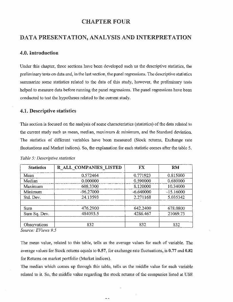
CHAPTER FOUR
DATA PRESENTATION, ANALYSIS AND INTERPRETATION
4.0. Introduction
Under this chapter, three sections have been developed such us the descriptive statistics, the
preliminary tests on data and, in the last section, the panel regressions. The descriptive statistics
summarize some statistics related to the data of this study, however, the preliminary tests
helped to measure data before running the panel regressions. The panel regressions have been
conducted to test the hypotheses related to the current study.
4,1. Descriptive statistics
This section is focused on the analysis of some characteristics (statistics) of the data related to
the current study such as mean, median, maximum & minimum, and the Standard deviation.
The statistics of different variables have been measured (Stock returns, Exchange rate
fluctuations and Market indices). So, the explanation for each statistic comes after the table 5.
Table 5: Descriptive statistics
Statistics R ALL COMPANIES LISTED FX RM
Mean 0.572464 0.771923 0.815000Median 0.000000 0.590000 0.680000Maximum 608.3300 8.120000 10.34000Minimum -96.27000 -6.640000 -15.16000Std.Dev. 24.13593 2.271168 5.035342
Observations 832 832 832
SumSum Sq. Dev.
476.2900484093.5
642.24004286.467
678.080021069.73
Source: EViews 9.5
The mean value, related to this table, tells as the average values for each of variable. The
average values for Stock returns equals to 0.57, for exchange rate fluctuations, is 0.77 and 0.82
for Returns on market portfolio (Market indices).
The median which comes up through this table, tells us the middle value for each variable
related to it. So, the middle value regarding the stock returns of the companies listed at USE
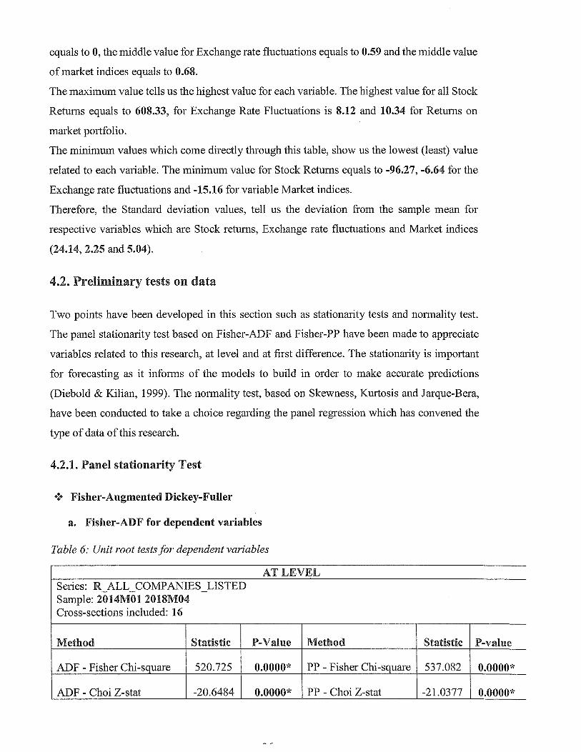
equals to 0, the middle value for Exchange rate fluctuations equals to 0.59 and the middle value
of market indices equals to 0.68.
The maximum value tells us the highest value for each variable. The highest value for all Stock
Returns equals to 608.33, for Exchange Rate Fluctuations is 8.12 and 10.34 for Returns on
market portfolio.
The minimum values which come directly through this table, show us the lowest (least) value
related to each variable. The minimum value for Stock Returns equals to -96.27, -6.64 for the
Exchange rate fluctuations and -15.16 for variable Market indices.
Therefore, the Standard deviation values, tell us the deviation from the sample mean for
respective variables which are Stock returns, Exchange rate fluctuations and Market indices
(24.14, 2.25 and 5.04).
4.2. Preliminary tests on data
Two points have been developed in this section such as stationarity tests and normality test.
The panel stationarity test based on Fisher-ADF and Fisher-PP have been made to appreciate
variables related to this research, at level and at first difference. The stationarity is important
for forecasting as it informs of the models to build in order to make accurate predictions
(Diebold & Kilian, 1999). The normality test, based on Skewness, Kurtosis and Jarque-Bera,
have been conducted to take a choice regarding the panel regression which has convened the
type of data of this research.
4.2.1, Panel stationarity Test
+ Fisher-Augmented Dickey-Fuller
a. Fisher-ADF for dependent variables
Table 6: Unit root tests for dependent variables
AT LEVELSeries: R ALL COMPANIES LISTEDSample: 2014M01 2018M04Cross-sections included: 16
Method Statistic P-Value Method Statistic P-value
ADF - Fisher Chi-square 520.725 0.0000* PP - Fisher Chi-square 537.082 0.0000*
ADF - Choi Z-stat -20.6484 0,0000* PP - Choi Z-stat -21.0377 0.0000*
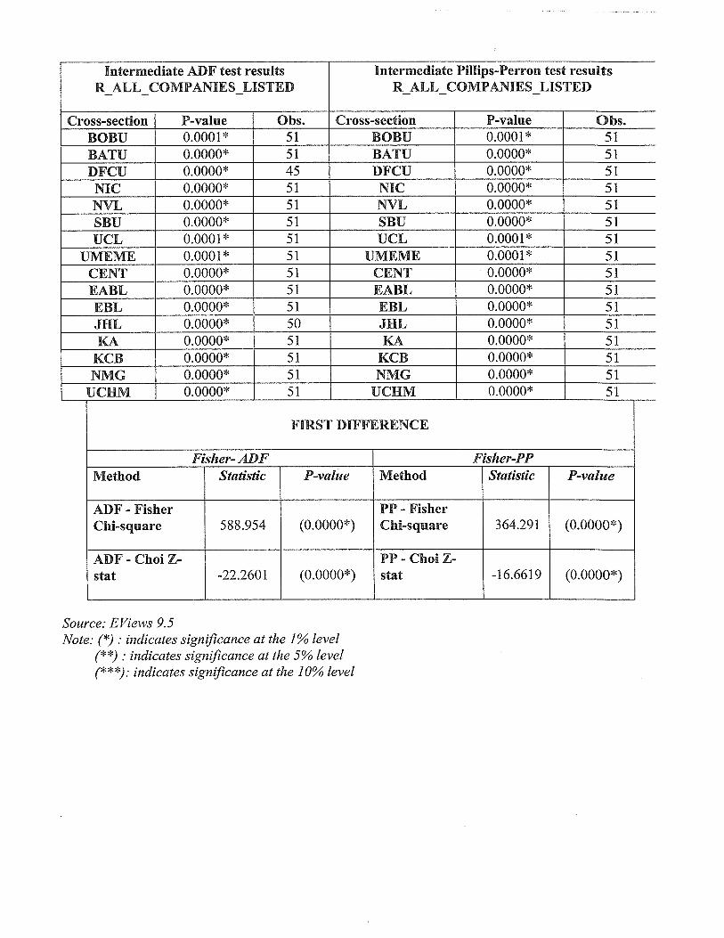
Intermediate ADF test results Intermediate Pillips-Perron test resultsR ALL COMPANIES LISTED RALL COMPANIES_LISTED
Cross-section P-value Obs. Cross-section P-value Obs.BOBU 0.0001* 51 BOBU 0.0001* 51BATU 0.0000* 51 BATU 0.0000* 51DFCU 0.0000* 45 DFCU 0.0000* 51NIC 0.0000* 51 NIC 0.0000* 51NVL 0.0000* 51 NVL 0.0000* 51SBU 0.0000* 51 SBU 0.0000* 51UCL 0.0001* 51 UCL 0.0001* 51
UMEME 0.0001* 51 UMEME 0.0001* 51CENT 0.0000* 51 CENT 0.0000* 51EABL 0.0000* 51 EABL 0.0000* 51EBL 0.0000* 51 EBL 0.0000* 51JHL 0.0000* 50 JIlL 0.0000* 51KA 0.0000* 51 KA 0.0000* 51
KCB 0.0000* 51 KCB 0.0000* 51NMG 0.0000* 51 NMG 0.0000* 51
UCHM 0.0000* 51 UCHM 0.0000* 51 —
FIRST DIFFERENCE
Fisher- ADF Fisher-PPMethod Statistic P-value Method Statistic P-value
ADF - Fisher PP - FisherChi-square 588.954 (0.0000*) Chi-square 364.291 (0.0000*)
ADF - Choi Z- PP - Choi Zstat -22.2601 (0.0000*) stat -16.6619 (0.0000*)
Source: EViews 9.5Note: (*) : indicates sign ificance at the 1% level
(**) : indicates sign~flcance at the 5% level(***): indicates significance at the 10% level
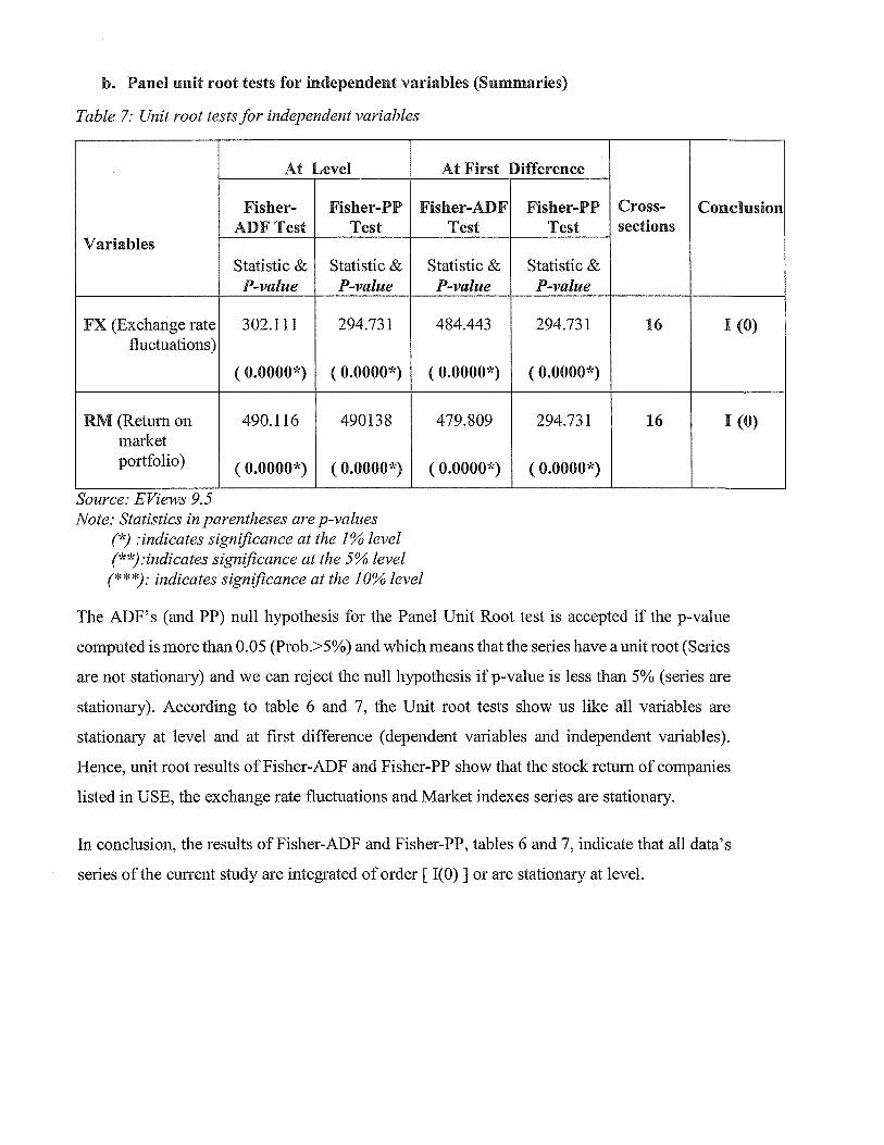
b. Panel unit root tests for independent variables (Summaries)
Table 7: Unit root tests for independent variables
At Level At First Difference
Fisher- Fisher-PP Fisher-ADF Fisher-PP Cross- ConclusionADF Test Test Test Test sections
VariablesStatistic & Statistic & Statistic & Statistic &P-value P-value P-value P-value
FX(Exchangerate 302.111 294.731 484.443 294.731 16 1(0)fluctuations)
( 0.0000*) ( 0.0000*) ( 0.0000k) ( 0.0000k)
RM(Returnon 490.116 490138 479.809 294.731 16 1(0)marketportfolio) ( 0.0000*) ( 0.0000*) ( 0.0000*) ( 0.0000*)
Source: EViews 9.5Note: Statistics in parentheses are p-values
(*) :indicates signijIcance at the 1% level(**):indicates sign~flcance at the 5% level(***): indicates sign~fIcance at the 10% level
The ADF’s (and PP) null hypothesis for the Panel Unit Root test is accepted if the p-value
computed is more than 0.05 (Prob.>5%) and which means that the series have a unit root (Series
are not stationary) and we can reject the null hypothesis if p-value is less than 5% (series are
stationary). According to table 6 and 7, the Unit root tests show us like all variables are
stationary at level and at first difference (dependent variables and independent variables).
Hence, unit root results of Fisher-ADF and Fisher-PP show that the stock return of companies
listed in USE, the exchange rate fluctuations and Market indexes series are stationary.
In conclusion, the results of Fisher-ADF and Fisher-PP, tables 6 and 7, indicate that all data’s
series of the current study are integrated of order [1(0) j or are stationary at level.
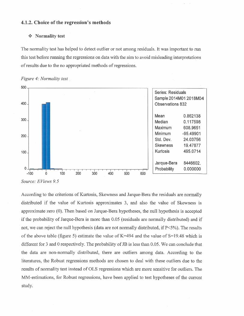
4.1.2. Choice of the regression’s methods
+ Normality test
The normality test has helped to detect outlier or not among residuals. It was important to run
this test before running the regressions on data with the aim to avoid misleading interpretations
of results due to the no appropriated methods of regressions.
Figure 4: Normality test
500 __________
Series: ResidualsSample 2014M01 201 8M04
400 Observations 832
Mean 0.862138Median 0.117598Maximum 608.9651
200 Minimum -95.49901Std. Dev. 24.03756Skewness 19.47877
ma Kurtosis 495.0714
Jarque-Bera 8446602.0 Probability 0.000000
-100 0 100 200 300 400 500 600
Source: EViews 9.5
According to the criterions of Kurtosis, Skewness and Jarque-Bera the residuals are normally
distributed if the value of Kurtosis approximates 3, and also the value of Skewness is
approximate zero (0). Then based on Jarque-Bera hypotheses, the null hypothesis is accepted
if the probability of Jarque-Bera is more than 0.05 (residuals are normally distributed) and if
not, we can reject the null hypothesis (data are not normally distributed, if P<5%). The results
of the above table (figure 5) estimate the value of K=494 and the value of S= 19.48 which is
different for 3 and 0 respectively. The probability of JB is less than 0.05. We can conclude that
the data are non-normally distributed, there are outliers among data. According to the
literatures, the Robust regressions methods are chosen to deal with these outliers due to the
results of normality test instead of OLS regressions which are more sensitive for outliers. The
MM-estimations, for Robust regressions, have been applied to test hypotheses of the current
study.
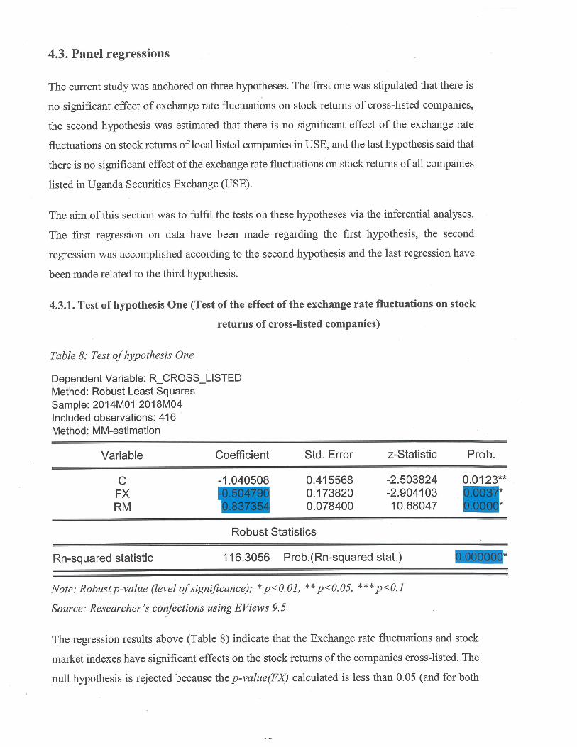
4.3. Panel regressions
The current study was anchored on three hypotheses. The first one was stipulated that there is
no significant effect of exchange rate fluctuations on stock returns of cross-listed companies,
the second hypothesis was estimated that there is no significant effect of the exchange rate
fluctuations on stock returns of local listed companies in USE, and the last hypothesis said that
there is no significant effect of the exchange rate fluctuations on stock returns of all companies
listed in Uganda Securities Exchange (USE).
The aim of this section was to fulfil the tests on these hypotheses via the inferential analyses.
The first regression on data have been made regarding the first hypothesis, the second
regression was accomplished according to the second hypothesis and the last regression have
been made related to the third hypothesis.
4.3.1. Test of hypothesis One (Test of the effect of the exchange rate fluctuations on stock
returns of cross-listed companies)
Table 8: Test ofhypothesis One
Dependent Variable: R_CROSS_LISTEDMethod: Robust Least SquaresSample: 2014M01 2018M04Included observations: 416Method: MM-estimation
Variable Coefficient Std. Error z-Statistic Prob.
C -1.040508 0.415568 -2.503824 0.0123**FX 050471 0.173820 -2.904103 ‘.00RM ‘:373 0.078400 10.68047 .000’
Robust Statistics
Rn-squared statistic 116.3056 Prob.(Rn-squared stat.) ‘.O’
Note: Robust p-value (level ofsignificance); *p<QQ], **p<Q~Q5, ***p<QjSource: Researcher’s confections using EViews 9.5
The regression results above (Table 8) indicate that the Exchange rate fluctuations and stock
market indexes have significant effects on the stock returns of the companies cross-listed. The
null hypothesis is rejected because the p-value(FX) calculated is less than 0.05 (and for both

independent variables). The alternative hypothesis is accepted regarding the figures which were
come through this table.
The p-value of the exchange rate fluctuations (FX) equals to 0.0037 which is less than 5%(The
decision rule of this study). In the same line, the coefficient’s value ofFX equals to -0.504790;
the (-) sign tells use the information of the elasticity of the exchange rate fluctuation vis-à-vis
the stock returns of the cross-listed companies. It means that for every one-unit increases in
exchange rate, a 0.504790-unit decrease in Stock returns of cross-companies, holding that all
other variables are remaining constant (Negative relationship). The p-value of the Returns on
Market portfolio equals to 0.0000 and the corresponding coefficient of 0.837354; the
coefficient of RIvI has a positive correlation with the stock returns of cross-listed companies
The robust probability [Prob.(Rn2-stat=0.000000)] is less than 5% which implies the goodness
of fit of the regression’s model.
The model related to the returns of cross-listed firms and exchange rate changes is fitted as
follow:
Rcrossiistea(PrediCted) = —1.040508 — 0.504790FX + 0.837354RM (1)
4.3.2. Test of hypothesis Two (Test of the effect of the exchange rate fluctuations on stock
returns of local-listed companies in USE)
Table 9: Test ofhypothesis Two
Dependent Variable: R_LOCAL_LISTED_UGMethod: Robust Least SquaresSample: 201 4M01 201 8M04Included observations: 416Method: MM-estimation
Variable Coefficient Std. Error z-Statistic Prob.
C -0.039204 0.126076 -0.310957 0.7558***FX -0.069537 0.052734 -1 .318647 0.1873***RM . 5 0.023785 2.334222 *
Robust Statistics
Rn-squared statistic 6.482276 Prob.(Rn-squared stat.) • 0 • I *
Note: Robust p-value (level ofsignificance); *p<0~Q1, **p<Q~05, ***p<QjSource: Researcher’s confections using EViews 9.5
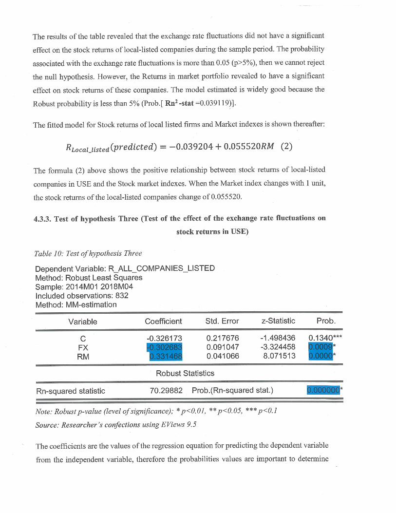
The results of the table revealed that the exchange rate fluctuations did not have a significant
effect on the stock returns of local-listed companies during the sample period. The probability
associated with the exchange rate fluctuations is more than 0.05 (p>5%), then we cannot reject
the null hypothesis. However, the Returns in market portfolio revealed to have a significant
effect on stock returns of these companies. The model estimated is widely good because the
Robust probability is less than 5% (Prob.[ Rn2 -stat =0.039119)].
The fitted model for Stock returns of local listed firms and Market indexes is shown thereafter:
RLocallisted(PrediCted) = —0.039204 + 0.055520RM (2)
The formula (2) above shows the positive relationship between stock returns of local-listed
companies in USE and the Stock market indexes. When the Market index changes with 1 unit,
the stock returns of the local-listed companies change of 0.055520.
4.3.3. Test of hypothesis Three (Test of the effect of the exchange rate fluctuations on
stock returns in USE)
Table 10: Test ofhypothesis Three
Dependent Variable: R_ALL_COMPANIES_LISTEDMethod: Robust Least SquaresSample: 2014M01 2018M04Included observations: 832Method: MM-estimation
Variable Coefficient Std. Error z-Statistic Prob.
C -0.326173 0.217676 -1.498436 0.1340***FX 0.30268 0.091047 -3.324458 l.000RM ‘.3 4 ; 0.041066 8.071513 ‘.00 e
Robust Statistics
Rn-squared statistic 70.29882 Prob.(Rn-squared stat.) ‘.OO’O
Note: Robust p-value (level ofsignificance); *p<Q~0J, **p<0~Q5, ***p<0~]Source: Researcher’s confections using EViews 9.5
The coefficients are the values of the regression equation for predicting the dependent variable
from the independent variable, therefore the probabilities values are important to determine
whether or not the null hypothesis can be rejected for given alpha level of significance (5%
related to this study).
The regression results above (Table 10) indicate that the Exchange rate fluctuations and stock
market indexes have significant effects on the stock returns of the companies listed in Uganda
Securities Exchange (USE). The null hypothesis is rejected because the p-value (FX) calculated
is less than 0.05 (for both independent variables). The alternative hypothesis is accepted
regarding the results of the table above. The p-value of the exchange rate fluctuations (FX) and
Market indexes (RM) equal to 0.0009 and 0.0000 respectively which are less than 5%. The
robust probability [Prob.(Rn2-stat =0.000000)] is less than 5% which implies that the goodness
of fit of the regression’s model.
The model related to the effect of exchange rate fluctuations on stock returns of the companies
listed in USE is fitted as follow:
RUSE(predicted) = —0.326173 — 0.302683FX + 0.33 1468RM (3)
The explanation about the above formula is that the coefficient’s value of FX equals to -
0.302683, the (-) sign stipulates the negative correlation between exchange rate fluctuations
and stock returns in USE (elasticity). It means that for every one percent increases in exchange
rate, a 0.302683 percent decrease in Stock returns in USE, holding that all other variables are
remaining constant. The corresponding coefficient for RM is 0.331468, that means the return
on market portfolio has a positive relationship with the stock returns of companies listed in
USE, when Stock market index increases with one unit, the stock returns of the companies
listed in USE increase with 0.331468.
CHAPTER FIVE
DISCUSSIONS, CONCLUSIONS, AND RECOMMENDATIONS
5.0. Introduction
This empirical research had a purpose to examine the effect of exchange rate fluctuations on
stock returns in Uganda Securities. Three objectives have been developed to achieve that
purpose. These objectives have been achieved through the findings of the current study.
Under this chapter, several sections have been developed particularly: discussion of major
findings, the conclusions and the recommendations.
5.1, Discussion of major findings
5.1.1. The effect of exchange rate fluctuations on stock returns of cross-listed companies).
The first objective of the current study was to examine the effect of exchange rate fluctuations
on stock returns of cross-listed companies. Ugandan stock market has eight companies that it
shares with the Kenyan stock market (Appendix I). The findings related to this objective
showed that the exchange rate fluctuations have significant effect on stock returns of the cross-
listed companies because the p-value associated to it was less than five percent. Then, we
rejected the null hypothesis which told us like the exchange rate fluctuations hadn’t the effect
on the Kenyan’s companies listed in USE. The coefficient’s sign of the exchange rate
fluctuation was negative which means that the exchange rate fluctuation and the stock returns
of these companies are negatively correlated; one percent of change in exchange rate can affect
negatively the stock returns of these firms with a value of the exchange rate fluctuation’s
coefficient.
This finding joins the study of Simakova (2017) who conducted a study on the impact of the
exchange rate movements on the companies listed in Czech, Hungary, Poland and Slovakia
stock markets, using a Jorion’ s model, all her time series used in her study revealed a negative
relationship between exchange rate and movement and the stocks returns in these countries’
stock markets. This finding is also related to the conclusion of Bodnar and Marton(2002), and
Tomanove (2016).
The Kenyan’ s companies which are quoted in Uganda Securities Exchange are more exposure
to Ugandan shilling’s rate changes and this affect severally their stock returns according to the
findings. On the other hand, return on market portfolio had also a significant effect on the stock
returns of these cross-listed companies, which is normal. The market Index is the weighted
average of the companies listed in a particular stock market; it implies that when the stock
market performs well, the impact of that performance can affect positively the firms listed on
that particular Stock exchange. This finding confirms the theories related to the stock exchange
(Chordia at al., 2014).
5.1.2. The effect of exchange rate fluctuations on stock returns of local-listed companies
in USE.
The second objective of this study was to examine the effect of exchange rate fluctuations on
stock returns of local listed companies in Uganda Securities Exchange. The Uganda’s firms
listed at USE are eight and there are in partnership with the eight Kenyan’ s companies which
are also listed in the same Stock market.
The findings related to this second objective estimate that the exchange rate fluctuations hadn’t
a significant effect on stock returns of local-listed companies in USE regarding our sample
period (January, 2014 - April, 2018) because the p-value associated to it was more than five
percent that why we accepted the null hypothesis. However, the return on market portfolio
showed a positive and significant effect on the stock returns of the local-listed companies with
a positive coefficient which means that when the market index change with one percent, the
stock returns of the local-listed companies in USE will also increase by the value of the return
on market portfolio’s coefficient.
This finding is also joined the results of Mugera (2013) who investigated on “the effect of
foreign exchange rate risk management on firm value of firms listed at NSE. He did not find a
significant impact of exchange rates on these companies.
5.1.3. The effect of exchange rate fluctuations on stock returns of firms listed in USE.
The third objective of this study was to examine the effect of the exchange fluctuations on the
stock returns of all companies quoted in Uganda Securities Exchange. The USE has 16 listed
companies; the 16 companies are subdivided into two types: we have 8 Ugandan companies
and 8 companies which are listed in both NSE and USE.
The findings demonstrate that the exchange rate fluctuations have a negative and a significant
effect on stock returns of the companies listed in USE. The probability value associated with
the exchange rate fluctuation was less than five percent which lead us to reject the null
hypothesis and accept the alternative hypothesis (The exchange rate changes have a significant
effect on stock returns in USE) but the market index has a positive and significant effect on the
stock returns in USE.
Many researchers tried to establish whether there is an effect of exchange rates on firms’
valuation; there have been mix-results: some authors found the effect of the exchange rate
fluctuations on stock returns (Shapiro, 1975, & Simakova, 2017) and others did not find any
effect (Bartram & Bodnar, 2012). That’s why we call it “the exchange rates’ Puzzle” (Bodnar
& Marston, 2002). Grouping firms by certain characteristics can lead to a less noisy estimation
(Simakova, 2017). The Panel regressions were subdivided into three categories: cross-listed
companies, local-listed companies, and whole companies (USE: 2014/01-2018/04).
The major finding for this study is that the exchange rate fluctuations have a negative and
significant effect on stock returns in USE due to the cross-listed companies with Nairobi
Security Exchange. Negative exposure coefficient suggests that the change of one unit in
exchange rate is followed by a decrease of firm’s stock returns. All robust models developed
had a goodness of fit which is quite high.
Regarding the puzzle of the link between exchange rate fluctuations and stock returns, the
results obtained from this study joined the group of researchers who have found the negative
correlation between exchange rate changes and stock returns such as Chapiro (1975),
Tomanova (2016), Simakova (2017), among others.
5.2. Conclusion
The purpose and objectives of this study have been achieved through different tests on data.
Company’s involvement in global activities through international trade is the primary source
of its foreign exchange exposure, but there are many factors which can cause the indirect
exposure as well. The aim of this paper was to evaluate the effect of exchange rate fluctuations
on stock returns in Uganda Securities Exchange. This study applies Jorion’s model and panel
data regression for the sample period 52 months (2014/01-2018/04). Panel data approach was
applied to pool the data across companies and time. The study takes into account also cross-

listed and local listed companies in USE what allows to test the effect of exchange rate
fluctuations on stock returns in USE. The preliminary tests from the USE monthly returns and
real exchange rates show the stationarity among series {I(O)}, positive skewness, leptokurtosis
(positive kurtosis), and non-normal distribution.
Regarding the purpose of this study, the findings of this study revealed a significant effect of
exchange rate movements on the stock returns of the companies listed in USE; then, level and
even direction of this effect differs across companies listed in USE.
According to the objective one, the findings demonstrated that the exchange rate fluctuations
had a negative and significant effect on stock returns of the cross-listed companies.
The objective two was achieved through the findings which showed that there is not a
significant effect of exchange rate fluctuations on stock returns of local-listed companies in
USE but I find a positive relationship between stock returns and return on market portfolio
which is normal.
Therefore, according to objective three, all estimations for the whole period and whole
companies listed in USE revealed negative and significant effect between exchange rate
fluctuations on of stock returns due to the cross-listed companies with Kenyan stock market.
Negative exposure coefficient suggests that if the exchange rate moves by one unit, the stock
returns in USE decrease by the amount of the coefficient of exchange rate factor. The highest
exchange exposure was observed in case of the cross-listed companies.
5.3. Recommendations
The findings of this study provide policy recommendations to regulators in Uganda.
The first objective of this study was to examine the effect of exchange rate fluctuations on
stock returns of cross-listed companies. Hence, this study is important to the government policy
makers as it informs the sensitivity of cross-border trade volatility, from the currency market
to the stock market. There is need for formulation of government policies that involve crossing
border asset effects. Policies of the introduction of the derivatives in the market should be
formulated in order to hedge against foreign exchange volatility in the Ugandan market. The
governor of USE could reduce information asymmetry through the Ugandan exchange.

However, the second objective of this study was to examine the effect of the exchange rate
fluctuations on stock returns of local-listed companies in USE. Uganda adopted the free-
floating exchange rate ate the beginning of 1 990s and the exchange rate is determined by the
market forces such as the supply and demand of the Ugandan currency, thus the Uganda
shilling is vulnerable with that because the Ugandan economy is not yet strong enough to face
directly the dollar or Euro currencies, I could propose the pegged float exchange rate regime
which can help the Governor of the Ugandan central bank to stabilize the nominal exchange
by issuing money or withdraw it at any time within the economy to stabilize the exchange rate;
the transmission mechanism through prices to the exchange rate is immediate. This could
protect Ugandan companies against foreign exchange rates risks. Also, the financial regulators
should increase the companies listed at this stock exchange, thus elevating the Uganda bourse
to a global level. This would increase the financial intermediation process that is an externality
effect of globalization and cross-border financial integration. Thereby, this will enable global
competitiveness that will attract foreign investments on the locally listed companies.
Besides, the third objective of this study was to examine the effect of the exchange rate
fluctuations on stock returns of all companies quoted in Uganda Securities Exchange (USE).
In the long run, exchange rate volatility cannot be controlled through the stock market
interventions. Therefore, financial market policy formulation is applicable in the short run. The
Bank of Uganda can develop instruments regarding the price dynamics and to reduce the
nominal interest rate because a change in the domestic money supply leads to a change in the
level of prices and a change in the level of prices leads to a change in the exchange rate, the
management of the monetary policy is very important to reduce the exchange rate fluctuations
in Uganda. The good management of the money supply can help to determine the exchange
rate, then the Uganda Central bank can focus it forces to manage the interest rate set and the
amount of money printed by the treasury. And thereby reduce the inflationary pressure due to
the increased amount of money in circulation which can lead to a devaluation of the currency.
Another recommendation derived from this study is the asset protection of small-scale
investors. An insurance scheme should be established in order to protect the small market
investors. Strict guidelines should be formulated to inform the market discipline of
stockbrokers and agencies amongst other intermediaries to minimize the risk of loss of
investments. This will enhance market integrity that will increase investor confidence and
increase the returns on investments.

5.4. Limitations of the study
The current study was dealing with the secondary data; clearly, the issues with data availability
are a significant constraint for student researchers due to the costs of internet conations and
also some websites asked money when we wanted to access some information about companies
listed at Ugandan Securities Exchange.
Regarding the theoretical limits, we could not gather all theories related to stock market returns
and exchange rate movements in this study that is the reason why we have focused only on two
popular theories related to stock returns and exchange rate fluctuations which are the Efficient
Market Hypothesis and the International Fisher Effect. In this particular case, the tests in this
study would have been more powerful if information about the currency denomination of
sources of revenue were available in addition to the currency denomination of liabilities.
5.5. Contribution to knowledge
In all, this study has advanced the literature, however modestly, in understanding the
mechanisms through which exchange rate fluctuation affects the stock returns in Lower
Developed Countries. The studies related to exchange rate fluctuations and stock returns in
LDCs are very few especially when it is regarding the stock exchange.
Flotta (2014) tried to analyze the impact of exchange rate movements on firm value in Mexico;
She used a sample of returns of non-financial firms but she found two results: The firms that
engage international activities are significantly less sensitive to the exchange rate movements
than firms that rely primary domestic sales. So, the current study had a gap with the work Flotta
in two points: first, this work analyzes the effect of exchange rate fluctuations on stock returns
in Ugandan area and the second fact the firms selected in the current work are financial and
non-financial firms. The results of these two works are very different by considering those
facts.
The current work is different from Simakova (2017) because his study analyzed the impact of
the exchange rate movements on firm values regarding the stock markets of four developed
countries, however the current study analyzes the effect of exchange rate fluctuations on stock
returns in LDCs (Lower Developed Countries) situations. Even if the conclusion of this study
was similar to the conclusion of Simakova but there is a gap between them regarding their
methodologies and approaches.
A (~
The originality of this study is that: first of all, it was analyzed the effect of exchange rate on
the stock returns in Uganda macroeconomic situations which is very different from Kenya and
from developed countries, the second aspect of this empirical research, it has analyzed the
effect of exchange rate fluctuations by grouping companies by certain characteristics (cross
listed and local listed companies). The findings of this research revealed the negative impact
of the foreign listed companies on Uganda’s listed companies regarding the exchange rate
exposure, the foreign companies shared their risks with the Ugandan companies and that could
affect the wealth of stakeholders. This study is different for others empirical researches
(Shapiro, 1975, Flota, 2014, Tomanova 2016, and Simakova, 2017) regarding the geographic
area, macroeconomic specificities of countries, specificity of the Stock Exchange, type of
companies and the appropriated analyses, and so on.
Due to the puzzling of the link between exchange rate fluctuations and stock returns (Bodnar
& Marston, 2002), this study has an important place in empirical and theoretical views because
it was joined the group of studies that have found a negative effect of the exchange rate
fluctuations on stock returns.
5,6, Areas of further research
This study was focused on the exchange rate fluctuations and stock returns in Uganda
Securities Exchange. Further research should be carried out on the hedging activities on the
exchange rate movements. This would investigate the effect of various hedging activities on
the foreign exchange market. Consequently, this should follow the various economic
transmission mechanisms so that it may be clear to define which channels can never be hedged
or which channel is easily to hedge. Further research can develop models on hedging markets
in a case to provide instruments which can help the companies to reduce the effect of exchange
rate on their stock returns because hedging against currency risk can change the character of
exchange rate exposure in significant way. The further research can conduct, also, the
investigations on the effect of the exchange rate fluctuations on stock returns by considering
the East Africa stock Markets (Kenya, Rwanda, South Soudan, Tanzania, and Uganda).
en
REFERENCES
Abdulla, M. (2017). Foreign (other countries) exchange turnover. Monetary and Economic
Department. (pdf). Retrieved from https ://www.bis.org/abdulla/
Abor, J. (2005). The effect of capital structure on profitability: An empirical analysis of listed
firms in Ghana. The Journal ofRisk Finance, 6(5), 438-445, retrieved from
doi:l0.l 108/15265940510633505
Adler, M., & Dumas, B. (1984). Exposure to currency risk: Definition and measurement.
Financial Management, 13(2): 41-50.
Akintoye, I., R. (2008). Efficient market hypothesis and behavioural finance: A review of
literature. European Journal ofSocial Sciences. 7(2), 7-17.
Allayannis, G., & Weston, J. (2001), The use of foreign currency derivatives and firm market
value. Review ofFinancial Studies, 14(1), 243-76.
Allen, H., L. & Taylor, M., P. (1990). “Charts, Noise, and Fundamentals Foreign Exchange
Markets.” Economic Journal~ 100, 49—59.
Amihud, Y. (2002). Illiquidity and stock returns: cross-section and time-series effects.
Journal ofFinancial Markets, 5(1), 31—56.
Ang, A., Hodrick, R., J., Xing, Y., & Zhang, X. (2006). The cross-section of volatility and
expected returns. Journal ofFinance, 61(1), 259—299.
Anyanzwa, J., (2016, August 20). New law passed, gives Uganda bourse nod to go public.
The EastAfrican. Nairobi. Retrieved from
http://www.theeastafrican.co.ke/business/Uganda-Securities-Exchange-get-nod-to-sell
shares-self-list/2560-33 51748-1 2qoteyz/index.html
Arnott, R., D., Hsu, J., & Moore, P. (2005). ‘tFundamental Indexation”. Financial Analysts
Journal, 60 (2): 83—99.
Bachelier, L. (1900), Théorie de la speculation, Annales ScientijIques de 1 ‘Ecole Normale
Supérieure Sér., 3(17), 21— 86.
Baganzi, R., Kim, B., G., & Shin, G., C. (2017). Portfolio optimization modelling with R for
enhancing decision making and prediction in case of Uganda Securities Exchange. Journal
ofFinancial Risk Management, 6, 325-351. doi:10.423 6/jfrm.20 17.64024
Baltagi, B., H. (2005). Econometric analysis ofpanel data. 3rd edition. West Sussex: Wiley.
Bartram, S. M., & Bodnar, G. M. (2012). Crossing the lines: The conditional relation between
exchange rate exposure and stock returns in emerging and developed markets, Journal of
International Money and Finance, 31, 766-792.
Bodnar, M., & Marston, C. (2002). Exchange rate exposure : A simple model. International
Finance Review, 3, 107-115.
Bourbonnais, R. (2009), Econométrie, Manuel et exercices corrigés, Paris éd. Dunod.
Buckley, A. (2004). Multinational Finance. Harlow, UK: Pearson Education Limited. ISBN
978-0-273-68209-7
Businge, J. (2014, February 14). Uganda Clays turnaround. The Independent. Retrieved from
https://web.archive.org!web/20 140310121021 /http://www.independent.co.ug/business/bus
iness-news/87 11 -uganda-clays-turnaround
Caramazza, F. & Aziz, J. (1998). Fixed or Flexible? Getting the Exchange Rate Right in the
1990s. Economic Issues, Washington D.C., USA. ISBN 1-55775-692-9
Chatterjee, S. & Mächler, M. (1995). Robust regression: A weighted least squares approach.
Communications in Statistics, Theoty and Methods, 26, 1381-1394.
Choi J., & Prasad A. (1995). Exchange risk sensitivity and its determinants: A Firm and
Industry Analysis of US. Multinationals. Financial Management, 24(3), 77-88.
Choi, I. (2001). Unit root tests for panel data. Journal ofInternational Money and Finance,
20, 249—272.
Chordia, T., Subrabmanyam, A., & Tong, Q. (2014). Have capital market anomalies
attenuated in the recent era of high liquidity and trading activity? Journal ofAccounting
and Economics 58(1), 41—58.
Chow, E. H., Lee, W. Y., & Solt, M. E. (1997). The exchange rate exposure of asset returns.
Journal ofBusiness, 70(1): 105-123.
Chue, K., & Cook, E. (2008). Emerging Market Exchange Rate Exposure. Journal of
Banking and Finance, vol. 32,no. 7,1349—1362.
Cohen, L., Manion, L., & Morison, K. (2000). Research Methods in Education. London:
Routledge Falmer.
Damodaran, A. (2002). Investment Valuation (2nd ed.). John Wiley and Sons, New York.
Dichev, I., & Piotroski, J. (2001), “The long-run stock returns following bond rating
changes”, Journal ofFinance, 56, pp. 173-203.
Dickey, D.A., & Fuller, W.A. (1979). “Distribution of the estimators for autoregressive time
series with a unit root”. Journal of the American Statistical Association, 74, 427—431.
Diebold, F. X. &Kilian, L. (1999), Unit toot tests are useful for selecting forecasting models,
Journal ofBusiness and Economic Statistics, 18, 265-273.
Dufey, G. (1972). Corporate finance and exchange rate variations. Financial Management,
1(2), 51 -7.
c,)

Economywatch. (2010, November 23). Stock market returns. Retrieved from
https://www.economywatch.comlstock-markets-in-world!returns.html
Emenike, K. 0. (2017) “Weak-form efficiency after global financial crisis: Emerging stock
market evidence”. Journal ofEmerging Market Finance, 16(1), 90-113.
Emenike, K., 0., & Kirabo, K., B., J. (2018). Empirical evaluation of weak-form efficient
market hypothesis in Ugandan Securities Exchange. Journal ofContemporary Economic
and Business Issues, 5(1), 35 — 50.
Essays, UK. (2013, November). The stock exchange ofEgypt. Retrieved from
https://www.ukessays.com/essays/international-studies/the-stock-exchange-of
egypt.php?vref=1
Eun, S., & Resnick, G. (2011). International Financial Management (6th Edition). New
York, NY: McGraw-Hill/Irwin. ISBN 978-0-07-803465-7.
EViews (Wed, 25 October 2017). Panel Unit Root Testing. retrieved July 24, 2018, from
http ://www.eviews.comlhelp/helpintro.html#page/content/advtimeser/Panel_Unit_Root_T
esting.html
Fama, E., F. (1970). Efficient capital markets: A review of theory and empirical work. The
Journal ofJmnance, 25(2), 383—417.
Fisher, I. (1930), The Theory ofInterest. New York: Macmillan.
Fixed exchange-rate system. (n.d.). Wikipedia. Retrieved from
https://en.wikipedia.org/wikilFixed_exchange-rate_system
Flota, C. (2014). The impact of exchange rate movements on firm value in emerging markets:
The case of Mexico. American Journal ofEconomics, 4(2A): 5 1—72.
doi: 10.5923/s.economics.201401 .05
Fraser, S., & Pantzaliz, C. (2004). Foreign exchange exposure of US multinational
corporations: a firm specific approach. Journal ofMultinational Financial Management,
14(3): 261—281.
Halm, G., N. (1977). Jamaica and the par-value system. Essays in internationalfinance (no.
120). International finance section, Princeton University, New Jersey.
Harder, 5. (2010). The Efficient Market Hypothesis and Its Application to Stock Markets.
GRIN Verlag. 1SBN9783640743766
Hatemi-J, A., & Irandoust, M. (2008). The Fisher effect: A Kalman Filter Approach to
detecting structural change. Applied Economics Letters, 15 (8), 619-624.
Hetemi-J, A. (2009). The International Fisher Effect: Theory and application. Investment
Management and Finance Innovations, 6(1)
Hlouskova, 3., & Wagner, M. (2006). The Performance of Panel Unit Root and Stationarity Tests:
Results from A Large Scale Simulation Study. Econometric Reviews, 25, p. 85-1 16.
Hodrick, J. (1978). An empirical analysis of the monetary approach to the determination of
the exchange rate. In Frenkel, J. A., & Johnson, H. G. (Eds.), The economics of exchange
rates (pp. 97-128). Reading, MA: Addison-Wesley.
Horn E., J. (2012, November 9). What is NASDAQ? Business News Daily Contributor.
Retrieved from https://www.businessnewsdaily.corn!3403-nasdaq.html
https://www.use.or.ug/listed-securities
Huber, P.3. (1973) Robust Regression: Asymptotics, conjectures and Monte Carlo. Annals of
Statistics, 1, 799-821. doi: 10.121 4/aos/l 176342503
Hur, J. (n.d.). History of the stock market. Retrieved July 17, 2018, from
https://bebusinessed.com/history/history-of-the-stock-market/.
Hutson, E., & Stevenson, S. (2010). Openness, hedging incentives and foreign exchange
exposure: a firm-level multi-country study. Journal ofInternational Business Studies,
41(1), 105—122.
IBTimes Staff Reporter. (2013). “East African Stock Exchange in the works to Merge
Buoyant, Profitable Markets”. lB Times. New York City. Retrieved 25 July 2015.
Investopedia Staff. (2018, January 12). What is the difference between the Dow and the
Nasdaq? Retrieved from https://www.investopedia.com!askJanswers/difference-between~
dow-and-nasdaq/
Irwin, A., D. (2013). The Nixon shock afler forty years: the import surcharge revisited. World
Trade Review, 12, 2956. doi:10.1017/51474745612000444
Jorion, P. (1990). The exchange rate exposure of US multinationals, Journal ofBusiness,
63(3), 331-345. doi: 10.1086/296510
Jorion, P. (1991). The pricing of exchange rate risk in the stock market, Journal ofFinancial
and Quantitative Analysis, 26, 363-376. doi: 10.2307/2331212
Kerlinger, N., & Rint, N. (1986). Foundations ofbehavioral research. London: Winston Inc.
Learn to invest. (n.d.). Return. Investopedia. Retrieved July 10, 2018, from
https://www.investopedia.comlterms/r/return.asp#ixzz5LFKk7XlF
Leeson, R. (2003). Ideology and the International Economy: The Decline andfall ofBretton
Woods. Basingstoke: Palgrave Macmillan.
Lehrman, L., E. (2011, August 15). The Nixon shock heard ‘round the world. Retrieved from
https://www.wsj.comlarticles/SB10001424053 111904007304576494073418802358
Leviatan, N. (1981). Monetary expansion and real exchange rate dynamics. Journal of
Political Economy 89 (December): 1218-1227.
List of African stock exchanges. (n.d.). Wikipedia. Retrieved July 6, 2018, from
https://en.m.wikipedia.org/wiki/List_of~African_stock_exchanges
Mack, C., A. (2016, October 31). Robust regression. Retrieved from
http://www.lithoguru.com/scientistlstatistics
Maddala, G.S., & Wu, S. (1999). A Comparative Study of unit root tests with panel data and
a New simple test. Oxford Bulletin ofEconomics and Statistics, 61, 631-652.
Mark, N. (2009). Changing monetary policy rules, learning, and real exchange rate dynamics,
Journal ofmoney, credit, and banking, September 2009, 1047-1070.
Market index. (n.d.). Investopedia. Retrieved April 15, 2018, from
https://www.investopedia.com/temis/mlmarketindex.asp#ixzz5EGYcwWHy
Marston, R.C. (2001). The effects of industry structure on economic exposure. Journal of
international money andfinance, April, 149-164.
Masinga, W., & Machira, P. (2013, July 9). East Africa hopes to have regional stock
exchange in a year - experts. London: Trust media. Retrieved from
https://allafrica.comlstories/201 307090331 .html
Maurya, R. (2016, July 7). Fundamental and technical analysis. Fundamentals of
Accounting. Retrieved from https://www.fundamentalsofaccounting.org/fundamental
technical-analysis/
Mbubi, A., M. (2013). The effect offoreign exchange rates on the financial performance of
firms listed at the Nairobi securities exchange. (Unpublished doctoral dissertation),
University of Nairobi D6 1/73069/2009
Monetary policy. (n.d.). Bank of Uganda. Retrieved 12 April 2018, from
hftps://www.bou.or.ug/bou/monetarypolicy/faqs.html
Mugera, W. B. (2013). The effect offoreign exchange risk management on the value offirms
listed at the Nairobi Securities Exchange. (Unpublished doctoral dissertation), the
University of Nairobi, School ofbusiness, October 2013.
Muhumuza, M. (2015). Automated stock market to start trading in May. Daily Monitor,
Kampala. Retrieved from http://www.monitor.co.ug/business/automated-stock-market-to
start-trading-in-may/68 8322-2613 044-5qxde6!index
Muhumuza, M., K. (2017, January 2). How cross-listed firms wiped Shs 4trillion off stock
market. Retrieved from http://www.monitor.co.ug/Business/Markets!Cross-listed-firms
wiped-Shs4-trillion-off-stock-market/688606-3 503 864-xbeh8alindex.html
Muller, A., & Verschoor, W. F. C. (2006). Asymmetric foreign exchange exposure: Evidence
from U.S. multinational firms. Journal ofEmpirical Finance, 13(4—5): 495—518.
Mwangi, W.G., (2013). The effect offoreign exchange risk management on financial
performance ofmicrofinance institutions in Kenya. (Unpublished doctoral dissertation),
the University ofNairobi, School of business, November 2013.
Nakamura, E., & Steinsson, J. (2018). Exchange rate regimes. Columbia, February 2018.
Nampeera, J. (2015). Foreign exchange risk management and performance of forex bureaus
in Uganda. (Unpublished doctoral dissertation), Makerere University, Business
administration, 201 3/HDO6/252 1 U
Neil J., 5. (2010). Ex post facto study. Encyclopedia ofResearch Design, Sage Research
Methods. doi:10.41 35/978141 2961 288.n145
O’Connell, J. (1968). “An T~ntemational Adjustment Mechanism with Fixed Exchange Rates”.
Economica. 35 (139): 274—282. doi:10.2307/2552303. JSTOR 2552303.
Oketch, M., L. (2011, January 4). “USE leads Sub-Saharan Africa in all shares index 2010”.
Daily Monitor. Kampala. Retrieved from
http://www.monitor.co.ug/Business/Prosper/6886 16-1 082848-hOsri d!index.html
Oketch, M., L. (2017, October 5). USE becomes public limited company. Daily Monitor.
Retrieved from http://www.monitor.co.ug!Business/USE-becomes-public-limited
company-!688322-4125718-1 Sdu4pm!index.html
Oluka, M. (2010, December). Firm characteristics, foreign exchange risk management and
performance a case ofexportfirms in Uganda. (Unpublished doctoral dissertation),
Makerere University, Accounting and Finance! 2006!HD 1 0!6009U
Onegi-Obel, G. (2016, October 23). Bank of Uganda governors and the capital markets
industry. The Observer (Uganda). Kampala. Retrieved from
http:fiwww.observer.ug!viewpoint!46007-bank-of-uganda-govemors-and-he-capital-
markets-industry
Pedroni, P. (2000). Fully modified OLS for heterogeneous cointegrated panels. Advances in
Econometrics, 15, 93—130.
Phillips, P., C., B, & Perron, P. (1988). Testing for a unit root in time series regression.
Biometrika, 75, 335—346.
Rapach, E., & Wohar, M. (2002). Testing the monetary model of exchange rate
determination: New evidence from a century of data. Journal ofInternational Economics,
58, 359-385. doi:10.1016/50022-1996(01)00170-2
Rees, W. & Unni, S. (2005). Exchange rate exposure among European firms: evidence from
France, Germany and the UK. Accounting and Finance, 45(3): 479—497.
Reilly, K., F. & Brown, C., K. (2008). Investment analysis andportfolio management. South
Western Cengage Learning (lOth Edition). Cenveo Publisher services.
Reinhart, C., M., & Rogoff, K., 5. (2004). “The Modem History of Exchange Rate
Arrangements: A Reinterpretation”. Quarterly Journal ofEconomics. 119 (1): 1—48.
doi:10.1 162/003355304772839515
Rousseeuw, P.J. and Yohai, V. (1984), “Robust Regression by Means of S estimators”, in
Robust and Nonlinear Time Series Analysis, edited by J. Franke, W. Härdle, and R.D.
Martin, Lecture Notes in Statistics 26, Springer Verlag, New York, 256-274.
Shafer, W., & Hugo, S. (1975). “Equilibrium in abstract economies without ordered
preferences,” Journal ofMathematical Economics, Elsevier, 2(3), 345-348, December.
Shapiro, A., & Rutenberg, D. (1976). Managing exchange risks in afloating world. Financial
Management, Summer, 48-5 8.
Shapiro, A.C. (1975). Exchange rate changes, inflation, and the value of the multinational
corporation. Journal of Finance, September, 485-502.
Shapiro, A.C. (2013). Multinationalfinancial management (lOth Ed). Hoboken, New Jersey:
Wiley.
~imaková, J. (2017). The impact of exchange rate movements on firm Value in Visegrad
countries. Acta Universitatis Agriculturae et Silviculturae Mendelianae Brunensis, 65(6),
2105—2111.
Stavárek, D. and Tomanová, L. (2014). Exchange rate volatility exposure on corporate cash
flows and stock prices: The case of Czech Republic. In: Proceeding ofthe 12th
International Scient~fl Conference on Economic Policy in the European Union Member
Countries. Karviná: Silesian University in Opava, School of Business Administration in
Karvina, 882 —890.
Stromberg, A. J. (2004). “Why write statistical software? The case of robust statistical
methods”. Journal ofStatistical Software. Department of Statistics, University of
Kentucky.
Sundqvist, E. (2002). An empirical investigation ofthe International Fisher Effect. Retrieved
from http://www.essays.se/essay/fb8c34Oc7aJ
Taruna, N. (2017, July 14). Valuation methods. The economic times. Retrieved from
https://economictimes.indiatimes.com!small-biz/resources/startup-handbook/valuation
methods/articleshow/5936840 1 .cms
The East African (2018, February 13). Uganda: Stock exchange takes $21 .5M drive after
foreign investor exit. Peril of Africa. Retrieved from http://perilofafrica.com/uganda
stock-exchange-takes-2 1 -5m-dive-after-foreign-investor-exit/
Thirunavukkarasu, A. (2006). Exchange rate fluctuation and firm value analysis of emerging
market multinationals. Southern New Hampshire University, 2500 North River Road,
Manchester, New Hampshire- 03106 USA.
Tomanova, L. (2016). Exchange rate volatility exposure on corporate cash flows and stock
prices: The case of Poland. Proceeding ofthe 14th Eurasia Business and Economics
Society Conference on Business Challenges in the Changing Economic Landscape, 1,
Zurich: Springer International Publishing, 273—285.
TradeCrowd. (2014). A history ofLondon Stock Exchange. Retrieved July 17, 2018, from
https://www.tradecrowd. corn/learn-to-trade/stocks/history-of-london-stock
exchange/#.W02 1 E8uEYOM
Turner, J., D., Ye, Q., & Walker C., B. (2018). Media Coverage and stock returns on the
London Stock Exchange, 1825—70. Review ofFinance, 22(4), 1605—1 629.
UALR. (n.d.). Efficient market hypothesis notes. Fin 3310 Holland. Retrieved July 8, 2018,
from https://ualr.edu/lcholland/fin33 1 0/f33 1 Oemh.html
Uganda Insurers Association. (2015, May 15). Capital markets: Opportunities for growth of
the insurance industry in Uganda. Retrieved from http://uia.co.ug/capital-rnarkets
opportunities-for-growth-of-the-insurance-industry-in-uganda!
Uganda Securities Exchange. (2018, May 12). Retrieved from https://www.use.or.ug/listing
on-use
Uganda Securities Exchange. (n.d.). Uganda Securities Exchange. Retrieved July 8, 2018,
from https://www.use.or.ug/content/background
Ward, S. (n.d.). Firm valuation approaches. Retrieved April 15, 2018, from
http://www.thebalancesmb.comlsusan-ward-2946932
Wayne, S., & Sonnenschein, H. (1975). Equilibrium in abstract economies without ordered
preferences. Journal ofMathematical Economics, 2, 345-348.
Yaw-Yih, W. (2004). Fluctuations ofexchange rate on the valuation ofmultinational
corporations as Taiwan ~ Samples. Central Taiwan University of Science and
Technology, Taiwan.

Yohai, V., J. (1987), “High Breakdown point and high efficiency robust estimates for
regression,” Annals ofStatistics, 15, 642-656.
Zaman, A., Rousseeuw, P., J., & Orhan, M. (2001). Econometric applications of high-
breakdown Robust regression techniques. Economics Letters, 71, 1-8. doi:10.1016/S0165-
1765(00)00404-3
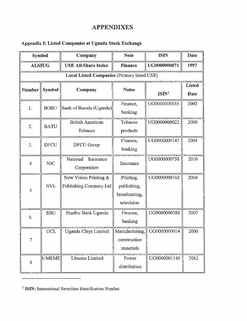
APPENDIXES
Appendix I: Listed Companies at Uganda Stock Exchange
Symbol Company Note [ ISIN Date
ALSIUG USE All-Share Index Finance UG0000000071 1997
Local Listed Companies (Primary listed USE)
ListedNumber Symbol Company Notes
151N1 Date
Finance, UG0000000055 20021. BOBU Bank of Baroda (Uganda)
banking
British American Tobacco UG0000000022 20002. BATU
Tobacco products
Finance, UG0000000147 20043. DFCU DFCU Group
banking
National Insurance UG0000000758 20104 NIC Insurance
Corporation
New Vision Printing & Printing, UG0000000162 2004
NVL Publishing Company Ltd publishing,
broadcasting,
television
6 SBU Stanbic Bank Uganda Finance, UG0000000386 2007banking
UCL Uganda Clays Limited Manufacturing, UG0000000014 2000
7 construction
materials
UMEME Umeme Limited Power UG0000001 145 20128
distribution
1 ISIN: International Securities Identification Number
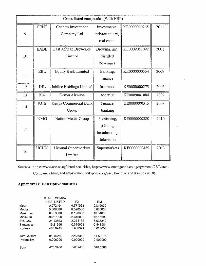
Cross-listed companies (With NSE)
CENT Centum Investment Investments, KE0000000265 2011
9 Company Ltd private equity,
real estate
EABL East African Breweries Brewing, gin, KE000908 1092 2001
10 Limited distilled
beverages
11 EBL Equity Bank Limited Banking, KE0000000554 2009finance
12 JHL Jubilee Holdings Limited Insurance KE0000000273 2006
13 KA Kenya Airways Aviation KE0009081084 2002
KCB Kenya Commercial Bank Finance, KE00000003 15 200814
Group banking
NMG Nation Media Group Publishing, KE0000000380 2010
15 printing,broadcasting,
television
16 UCHM Uchumi Supermarkets Supermarkets KE0000000489 2013Limited
Sources: https://www.use.or.ug/listed-securities, https://www.cmauganda.co.ugluglsmenu/23/Listed-
Companies.html, and https://www.wikipedia.orgluse, Emenike and Kirabo (2018).
Appendix II: Descriptive statistics
R_ALL_COMPANIES_LISTED FX RM
Mean 0.572464 0.771923 0.815000Median 0.000000 0.590000 0.680000Maximum 608.3300 8.120000 10.34000Minimum -96.27000 -6.640000 -15.16000Std. Dev. 24.13593 2.271168 5.035342Skewness 19.21356 0.370603 -0.543984Kurtosis 485.9945 5.988371 3.624008
Jarque-Bera 8138359. 328.6313 54.53275Probability 0.000000 0.000000 0.000000
Sum 476.2900 642.2400 678.0800
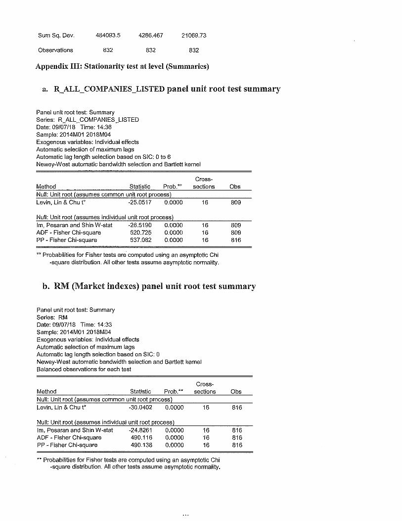
Sum Sq. Dev. 484093.5 4286.467 21069.73
Observations 832 832 832
Appendix III: Stationarity test at level (Summaries)
a. R_ALL_COMPANIES_LISTED panel unit root test summary
Panel unit root test: SummarySeries: R_ALL_COMPANIES_LISTEDDate: 09/07/18 Time: 14:36Sample: 2014M01 2018M04Exogenous variables: Individual effectsAutomatic selection of maximum lagsAutomatic lag length selection based on SIC: 0 to 6Newey-West automatic bandwidth selection and Bartlett kernel
Cross-Method Statistic Prob.** sections ObsNull: Unit root (assumes common unit root process)Levin, Lin & Chu t* -25.0517 0.0000 16 809
Null: Unit root (assumes individual unit root process)Im, Pesaran and Shin W-stat -26.51 90 0.0000 16 809ADF - Fisher Chi-square 520.725 0.0000 16 809PP - Fisher Chi-square 537.082 0.0000 16 816
** Probabilities for Fisher tests are computed using an asymptotic Chi
-square distribution. All other tests assume asymptotic normality.
b. RM (Market indexes) panel unit root test summary
Panel unit root test: SummarySeries: RMDate: 09/07/18 Time: 14:33Sample: 2014M01 2018M04Exogenous variables: Individual effectsAutomatic selection of maximum lagsAutomatic lag length selection based on SIC: 0Newey-West automatic bandwidth selection and Bartlett kernelBalanced observations for each test
Cross-Method Statistic Prob.** sections ObsNull: Unit root (assumes common unit root process)Levin, Lin & Chu t~ -30.0402 0.0000 16 816
Null: Unit root (assumes individual unit root process)Im, Pesaran and Shin W-stat -24.8261 0.0000 16 816ADF - Fisher Chi-square 490.116 0.0000 16 816PP - Fisher Chi-square 490.138 0.0000 16 816
** Probabilities for Fisher tests are computed using an asymptotic Chi-square distribution. All other tests assume asymptotic normality.
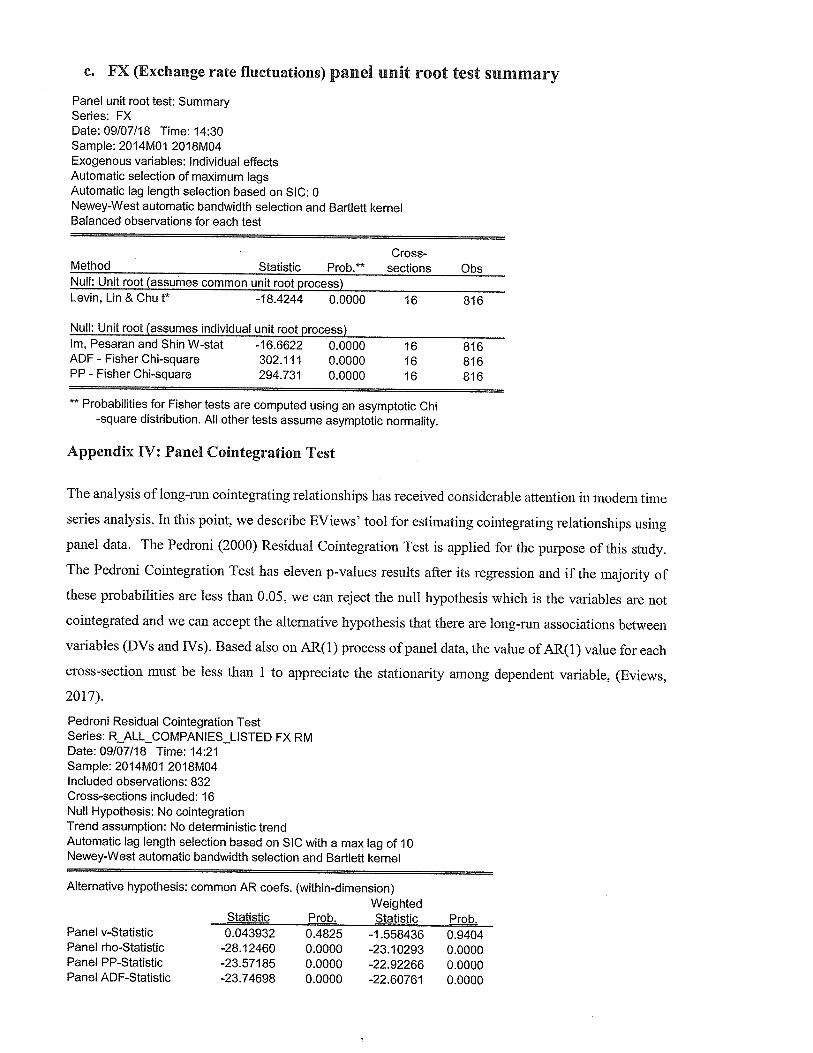
c. FX (Exchange rate fluctuations) panel unit root test summary
Panel unit root test: SummarySeries: FXDate: 09107/18 Time: 14:30Sample: 2014M01 2018M04Exogenous variables: Individual effectsAutomatic selection of maximum lagsAutomatic lag length selection based on SIC: 0Newey-West automatic bandwidth selection and Bartlett kernelBalanced observations for each test
Cross-Method Statistic Prob.** sections ObsNull: Unit root (assumes common unit root process)Levin, Lin & Chu t~ -18.4244 0.0000 16 816
Null: Unit root (assumes individual unit root process)Im, Pesaran and Shin W-stat -16.6622 0.0000 16 816ADF - Fisher Chi-square 302.111 0.0000 16 816PP - Fisher Chi-square 294.731 0.0000 16 816
** Probabilities for Fisher tests are computed using an asymptotic Chi
-square distribution. All other tests assume asymptotic normality.
Appendix IV: Panel Cointegration Test
The analysis of long-run cointegrating relationships has received considerable attention in modern time
series analysis. In this point, we describe EViews’ tool for estimating cointegrating relationships using
panel data. The Pedroni (2000) Residual Cointegration Test is applied for the purpose of this study.
The Pedroni Cointegration Test has eleven p-values results afier its regression and if the majority of
these probabilities are less than 0.05, we can reject the null hypothesis which is the variables are not
cointegrated and we can accept the alternative hypothesis that there are long-run associations between
variables (DVs and IVs). Based also on AR(1) process of panel data, the value of AR( 1) value for each
cross-section must be less than 1 to appreciate the stationarity among dependent variable, (Eviews,
2017).
Pedroni Residual Cointegration TestSeries: R_ALL_COMPANIE5 LISTED FX RMDate: 09/07/18 Time: 14:2 1Sample: 2014M01 2018M04Included observations: 832Cross-sections included: 16Null Hypothesis: No cointegrationTrend assumption: No deterministic trendAutomatic lag length selection based on SIC with a max lag of 10Newey-West automatic bandwidth selection and Bartlett kernel
Alternative hypothesis: common AR coefs. (within-dimension)Weighted
Statistic P rob. Statistic Prob.Panel v-Statistic 0.043932 0.4825 -1.558436 0.9404Panel rho-Statistic -28.12460 0.0000 -23.10293 0.0000Panel PP-Statistic -23.571 85 0.0000 -22.92266 0.0000Panel ADF-Statistic -23.74698 0.0000 -22.60761 0.0000

Alternative hypothesis: individual AR coefs. (between-dimension)
Statistic Prob.Group rho-Statistic -22.86574 0.0000Group PP-Statistic -27.16362 0.0000Group ADF-Statistic -25.86212 0.0000
Cross section specific results
Phillips-Peron results (non-parametric)
Cross ID AR(1) Variance HAC Bandwidth ObsBOBU 0.189 13.63655 13.51257 3.00 51BATU -0.154 29.88733 34.54788 3.00 51DFCU -0.066 61 .65772 59.99838 3.00 51
NIC -0.305 75.79724 97.89180 3.00 51NVL -0.214 3.609759 3.823248 2.00 51SBU -0.137 21.33272 16.40823 7.00 51UCL 0.321 89.74142 90.1 1207 2.00 51
UMEME 0.294 26.43995 25.76512 3.00 51CENT -0.032 46.06306 44.52825 2.00 51EABL -0.078 13.13770 12.32428 3.00 51EBL -0.121 7251.859 9212.421 3.00 51JHL -0.155 44.19843 34.77926 3.00 51KA 0.178 397.3548 447.6341 2.00 51
KCB -0.304 40.11456 33.77710 2.00 51NMG -0.047 55.22135 38.83741 7.00 51
UCHM -0.081 332.1948 332.1948 0.00 51
Augmented Dickey-Fuller results (parametric)
Cross ID AR(1) Variance Lag Maxlag ObsBOBU 0.189 13.63655 0 10 51BATU -0.369 20.65160 3 10 48DFCU -0.066 61.65772 0 10 51
NIC -0.305 75.79724 0 10 51NVL -0.214 3.609759 0 10 51SBU -0.137 21.33272 0 10 51UCL 0.321 89.74142 0 10 51
UMEME 0.294 26.43995 0 10 51CENT -0.032 46.06306 0 10 51EABL -0.078 13.13770 0 10 51EBL -0.121 7251.859 0 10 51JHL -0.155 44.19843 0 10 51KA 0.178 397.3548 0 10 51
KCB -0.304 40.11456 0 10 51NMG -0.047 55.22135 0 10 51
UCHM -0.081 332.1948 0 10 51
Appendix V: Regressions (Panel)
a) Regression related to cross-listed companies
Dependent Variable: R_CROSS_LISTEDMethod: Robust Least Squares
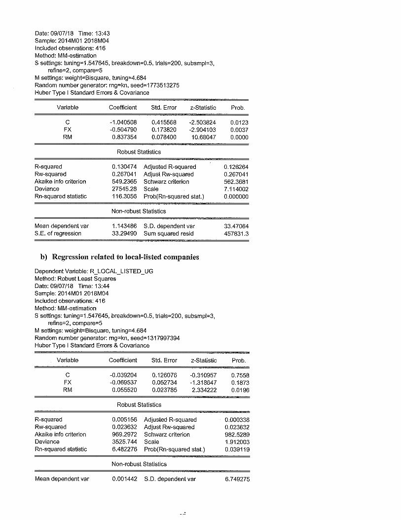
Date: 09/07/18 Time: 13:43Sample: 2014M01 2018M04Included observations: 416Method: MM-estimationS settings: tuning=1 .547645, breakdown=0.5, trials=200, subsmpl=3,
reflne=2, compare=5M settings: weight=Bisquare, tuning=4.684Random number generator: rng=kn, seed=1 773513275Huber Type I Standard Errors & Covariance
Variable Coefficient Std. Error z-Statistic Prob.
C -1 .040508 0.415568 -2.503824 0.0123FX -0.504790 0.173820 -2.904103 0.0037RM 0.837354 0.078400 10.68047 0.0000
Robust Statistics
R-squared 0.130474 Adjusted R-squared 0.126264Rw-squared 0.267041 Adjust Rw-squared 0.267041Akaike info criterion 549,2365 Schwarz criterion 562.3681Deviance 27545.28 Scale 7.114002Rn-squared statistic 116.3056 Prob(Rn-squared stat.) 0.000000
Non-robust Statistics
Mean dependent var 1.143486 S.D. dependent var 33.47064S.E. of regression 33.29490 Sum squared resid 457831.3
b) Regression related to local-listed companies
Dependent Variable: R_LOCAL_LISTED_UGMethod: Robust Least SquaresDate: 09/07/18 Time: 13:44Sample: 2014M01 2018M04Included observations: 416Method: MM-estimationS settings: tuning=1 .547645, breakdown=0.5, trials=200, subsmpl=3,
reflne=2, compare=5M settings: weight=Bisquare, tuning=4.684Random number generator: rng=kn, seed=1 317997394Huber Type I Standard Errors & Covariance
Variable Coefficient Std. Error z-Statistic Prob.
C -0.039204 0.126076 -0.310957 0.7558FX -0.069537 0.052734 -1 .318647 0.1873RM 0.055520 0.023785 2.334222 0.0196
Robust Statistics
R-squared 0.005156 Adjusted R-squared 0.000338Rw-squared 0.023632 Adjust Rw-squared 0.023632Akaike info criterion 969.2972 Schwarz criterion 982.5289Deviance 3525.744 Scale 1.912003Rn-squared statistic 6.482276 Prob(Rn-squared stat.) 0.039119
Non-robust Statistics
Mean dependent var 0.001442 S.D. dependent var 6.749275
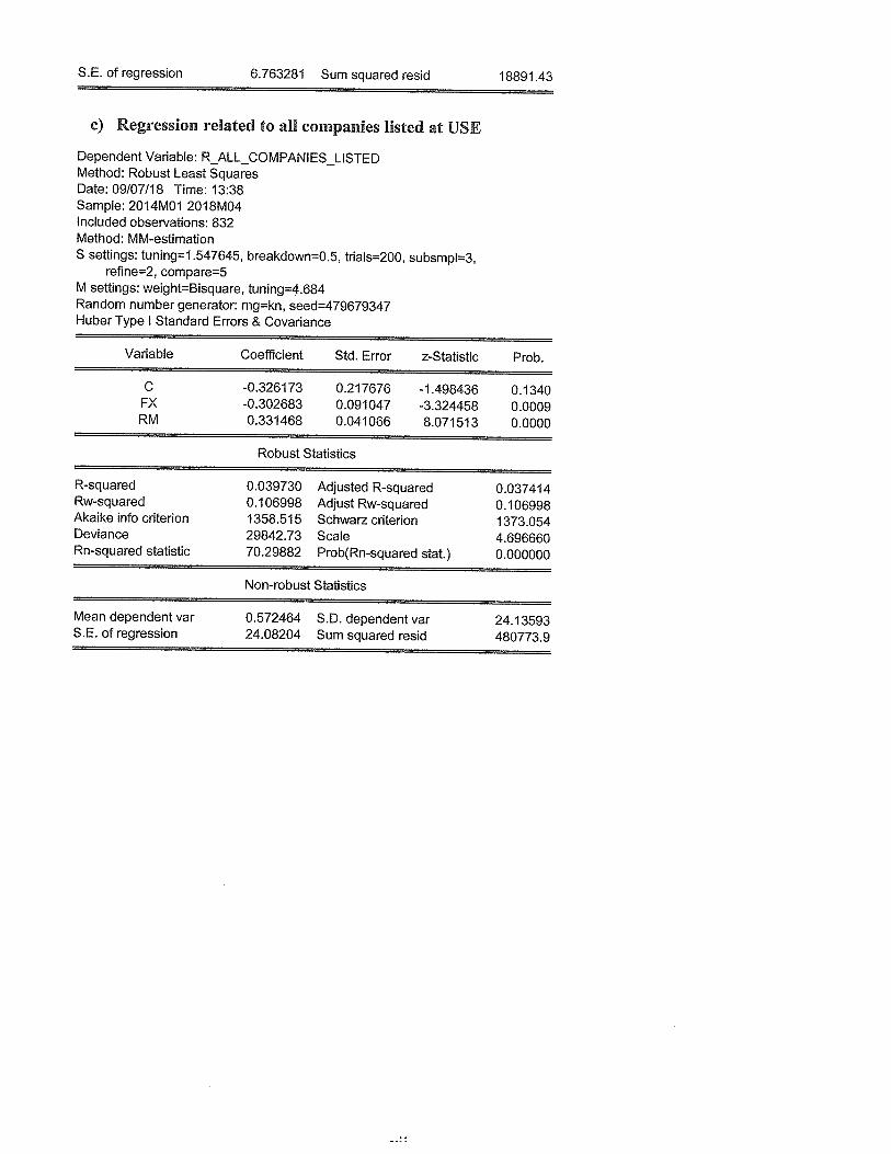
S.E. of regression 6.763281 Sum squared resid 18891.43
c) Regression related to all companies listed at USE
Dependent Variable: R_ALL_COMPANIES LISTEDMethod: Robust Least SquaresDate: 09/07/18 Time: 13:38Sample: 2014M01 2018M04Included observations: 832Method: MM-estimationS settings: tuning=1 .547645, breakdown=O.5, trials=200, subsmpl=3,
refine=2, compare=5M settings: weight=Bisquare, tuning=4.684Random number generator: mg=kn, seed=479679347Huber Type I Standard Errors & Covariance
Variable Coefficient Std. Error z-Statistic Prob.
C -0.326173 0.217676 -1.498436 0.1340FX -0.302683 0.091047 -3.324458 0.0009RM 0.331468 0.041066 8.071513 0.0000
Robust Statistics
R-squared 0.039730 Adjusted R-squared 0.037414Rw-squared 0.106998 Adjust Rw-squared 0.106998Akaike info criterion 1358.515 Schwarz criterion 1373.054Deviance 29842.73 Scale 4.696660Rn-squared statistic 70.29882 Prob(Rn-squared stat.) 0.000000
Non-robust Statistics
Mean dependent var 0.572464 S.D. dependent var 24.13593S.E. of regression 24.08204 Sum squared resid 480773.9


