Montclair State University Montclair State University
Montclair State University Digital Montclair State University Digital
Commons Commons
Theses, Dissertations and Culminating Projects
5-2018
Geochemical and Sedimentological Analysis of Marine Sediments Geochemical and Sedimentological Analysis of Marine Sediments
from ODP Site 696 and Implications for the Onset of Antarctic from ODP Site 696 and Implications for the Onset of Antarctic
Glaciation Glaciation
Allison Paige Lepp Montclair State University
Follow this and additional works at: https://digitalcommons.montclair.edu/etd
Part of the Environmental Sciences Commons
Recommended Citation Recommended Citation Lepp, Allison Paige, "Geochemical and Sedimentological Analysis of Marine Sediments from ODP Site 696 and Implications for the Onset of Antarctic Glaciation" (2018). Theses, Dissertations and Culminating Projects. 140. https://digitalcommons.montclair.edu/etd/140
This Thesis is brought to you for free and open access by Montclair State University Digital Commons. It has been accepted for inclusion in Theses, Dissertations and Culminating Projects by an authorized administrator of Montclair State University Digital Commons. For more information, please contact [email protected].

i
ABSTRACT
The Eocene-Oligocene Transition (EOT) approximately 34 million years ago
(Ma) marks the shift from the warm greenhouse conditions of the Eocene to today’s
icehouse, and was accompanied by the establishment of the East and West Antarctic Ice
Sheets. Details surrounding the timing, magnitude, and regional expansion of glaciation
are poorly constrained primarily due to low core recovery and lack of reliable age
models, and therefore warrant continued investigation. A recently updated age model
applied to Ocean Drilling Program (ODP) Site 696, located in the northwest sector of the
Weddell Sea, indicates Core 55R represents a high-recovery succession encompassing
the EOT. This project presents a high-resolution, multimethod analysis of this sediment
core.
Laser particle size analysis was performed throughout the core, and inductively
coupled plasma mass spectrometry and optical emission spectrometry are used to
quantify major, trace, and rare earth elemental concentrations on samples with >80%
mud. Paleoclimate proxies are calculated to characterize the dominant weathering regime
and degree of glacial influence on sediment. Results indicate a cool, dry climate and
sediment with a strong glacial signature, as evidenced by low chemical index of alteration
(CIA) values and significant contribution of glacial rock flour. Trace and REE ratios do
not suggest major changes in source material, and felsic versus mafic plots indicate 55R
sediment is felsic to intermediate in composition. Sediment remains well sorted
throughout, and therefore elemental enrichments are likely related to grain-size
partitioning.
ii
Results of this study have implications for the investigation into continental
glacial history of Antarctic through the EOT; 55R sediments reflect a similar climate to
shelf sediments retrieved from Prydz Bay and Wilkes Land Margins and are consistent
with significant terrestrial cooling across East Antarctica during the late Eocene. Studies
from West Antarctica, however, suggest a later onset with less glacial stability. Similar
high-resolution studies are thusly needed to further improve our understanding of
Antarctic ice dynamics in response to climate perturbations.
iv
Geochemical and Sedimentological Analysis of Marine Sediments from ODP Site 696 and Implications for the Onset of Antarctic Glaciation
A THESIS
Submitted in partial fulfillment of the requirements
for the degree of Master of Science
by
ALLISON PAIGE LEPP
Montclair State University
Montclair, NJ
2018

v
Copyright © 2018 by Allison Paige Lepp. All rights reserved.
vi
ACKNOWLEDGEMENTS
I first need to extend gratitude to my thesis sponsor, Dr. Sandra Passchier, for
being so much more than a research advisor during my time at Montclair. Thank you for
believing in my potential based on just a few emails and a grad school application. Many
of the opportunities I’ve had at MSU would not have been possible if not for you; thank
you for the guidance, the advice, the support, and for always having an open door (even
when it’s closed). This project was partially funded from NSF awards EAR 1531719,
ANT 1245283.
To Dr. Stefanie Brachfeld, for agreeing to serve on my committee despite the
abundance of responsibilities that come with a new position as Associate Dean. Your
expertise and genuine interest in your students are so appreciated. And to Dr. Xiaona Li,
for your patience and optimism in the lab. The quality of this research data would not be
where it is without your dedication and assistance. I’d also like to recognize Dylan Cone
for providing his particle size data.
Of course, a huge thank you to my mom and dad, for always supporting my
ambitions and curiosities, wherever they might lead me. To my friends for listening (or
pretending to listen) to me talk about Antarctica over the past two years: thank you. Also,
sorry. I’m forever grateful for those who made the time to visit and bring me reminders
of the South (Peter, Schyler, Zak, Erica, Kyle, Bolt). To April and Jenny, for helping me
fight off the “imposter syndrome”, even from hundreds of miles away. Finally, to Avery
and Zena, for so many Skype sessions and phone calls when I felt completely lost. I’m
eternally grateful.
vii
TABLE OF CONTENTS
Abstract ............................................................................................................................... i
Acknowledgements ........................................................................................................... vi
Table of Contents ............................................................................................................. vii
List of Figures ................................................................................................................... ix
List of Tables .................................................................................................................... xi
1. INTRODUCTION ....................................................................................................... 1
1.1 Background ...................................................................................................... 1
1.1.1 Evidence of the EOT ......................................................................... 1
1.1.2 Development of Antarctic Ice Sheets ................................................ 4
1.2 Study Location ................................................................................................. 6
1.2.1 ODP Site 696 .................................................................................... 6
1.2.2 Weddell Sea Sector Tectonics and Geology ...................................... 9
1.3 Age Model ..................................................................................................... 12
2. METHODOLOGY .................................................................................................... 13
2.1 Sedimentological Analysis ............................................................................. 13
2.1.1 Sample Selection ............................................................................. 15
2.1.2 Sample Preparation ........................................................................ 17
2.1.3 Data acquisition and processing .................................................... 18
2.2 Geochemical Analysis ................................................................................... 19
2.2.1 Sample Selection ............................................................................. 20
2.2.2 Sample Preparation ........................................................................ 20
2.2.3 Data acquisition and processing .................................................... 21
2.3 Paleoenvironmental Proxies and Ratios ..........................................................22
2.3.1 Ice-Rafted Debris Mass Accumulation Rate ................................... 22
2.3.2 Chemical Index of Alteration .......................................................... 24
2.3.3 Elemental Enrichments ................................................................... 24
2.3.4 Provenance Constraints .................................................................. 25
viii
3. RESULTS ................................................................................................................... 26
3.1 Particle Size Distributions .............................................................................. 26
3.2 Geochemistry ................................................................................................. 30
3.2.1 Paleoenvironmental Proxies ........................................................... 30 IRD MAR CIA
3.2.2 Elemental Enrichments ................................................................... 33
3.2.3 Provenance Constraints .................................................................. 36
4. DISCUSSION ............................................................................................................. 42
4.1 Paleoclimate Conditions ................................................................................ 42
4.1.1 Depositional Environment .............................................................. 42
4.1.2 Weathering Regime ......................................................................... 44
4.1.3 Particle Size Distributions .............................................................. 46
4.2 Sediment Source ............................................................................................ 48
4.2.1 Provenance ..................................................................................... 48
4.2.2 IRD MAR ........................................................................................ 49
4.2.3 Elemental Enrichments ................................................................... 51
5. CONCLUSION .......................................................................................................... 54
6. REFERENCES ........................................................................................................... 56
7. APPENDIX ................................................................................................................. 62
ix
LIST OF FIGURES
FIGURE 1. Global oxygen and carbon isotope composite record from Zachos et al. (2001) ................................................................................................................................. 2
FIGURE 2. Coupled global climate and ice growth models showing possible expansion
of Antarctic ice sheets during the EOT (DeConto and Pollard, 2003) .............................. 5
FIGURE 3. Map of East and West Antarctica with Site 696 drill site location ............... 8
FIGURE 4. Weddell Sea sector tectonics from 40 Ma to present (Carter et al., 2016) .. 10
FIGURE 5. Weddell Sea sector geologic formations ..................................................... 11
FIGURE 6. Site 696 age model ...................................................................................... 14
FIGURE 7. Age and depth of Core 55R in relation to downhole 696B cores ................ 14
FIGURE 8. Age model applied to Core 55R by section and depth ................................ 16
FIGURE 9. Downcore 55R grain size percentages, IRD MAR, and uniformity ........... 27
FIGURE 10. Ternary grain size distribution diagram for 55R samples ......................... 28
FIGURE 11. Particle size distribution by volume percent of 55R by section ................ 29
FIGURE 12. IRD MAR and IRD fraction comparison plot ........................................... 31
FIGURE 13. Chemical Index of Alteration against depth .............................................. 31
FIGURE 14. Rb/Cs versus Rb weathering plot (McLennan, 2001) ............................... 32
FIGURE 15. 55R trace element enrichments against upper continental crust values (McLennan, 2001) ............................................................................................................ 34
FIGURE 16. 55R rare earth element enrichments against average chondrite values (Nakamura, 1974) ............................................................................................................ 35
FIGURE 17. Ti/Al and Ti/Sc provenance evaluation plot .............................................. 37
FIGURE 18. Th/Sc versus Zr/Cr plot to examine mafic or felsic nature of 55R sediments ........................................................................................................................................... 38
FIGURE 19. Th/U versus Th plot comparing 55R samples to turbidite muds from various tectonic settings (McLennan, 2001) .................................................................... 39
FIGURE 20. Th/Ni versus Zr/Cr plot comparing 55R samples to Weddell Sea sector formations ........................................................................................................................ 41
FIGURE 21. La/Th versus Hf plot comparing 55R samples to Weddell Sea sector formations ........................................................................................................................ 41
FIGURE 22. Ternary grain size distribution diagram comparing 55R sediments to downcore samples ............................................................................................................ 43
x
FIGURE 23. Sand and silt distributions emphasizing regular increases in sand percent ........................................................................................................................................... 47
FIGURE 24. Grain size distribution for samples showing elevated Rb/Cs ratio ........... 52
FIGURE 25. Grain size distribution for samples showing elevated La/Th ratio ............ 52
FIGURE 26. Th/Sc versus Zr/Sc plot to examine degree of sediment recycling (McLennan et al., 1993) ................................................................................................... 53
FIGURE A.1. 55R major element enrichments against values of the North American Shale Composite (NASC; Gromet, 1984) ........................................................................ 62
xi
LIST OF TABLES
TABLE A.1 Complete list of sample IDs with corresponding depths (mbsf), ages (Ma), and particle size percents ................................................................................................. 63
TABLE A.2 List of samples that received modified preparation for laser particle size analysis ............................................................................................................................. 67
TABLE A.3 Trace element composition in ppm by section ........................................... 68
TABLE A.4 Rare earth element composition in ppm by section .................................... 71
TABLE A.5 Major element composition in normalized weight percent oxides by section ........................................................................................................................................... 74
1
1. INTRODUCTION
1.1 Background
The Eocene-Oligocene Transition (EOT) approximately 34 million years ago
(Ma) signifies a global climactic shift from a warm greenhouse to the present-day
icehouse. This shift was notably accompanied by a dramatic drop in global sea level
(Stocchi et al., 2013), a decrease in atmospheric carbon dioxide concentration (Pearson et
al., 2009; Pagani et al., 2005), reduction in terrestrial biodiversity and vegetation
(Anderson et al., 2011; Francis et al., 2009), and the development of the modern-day
Antarctic Ice Sheet (Coxall and Wilson, 2011). Recent literature agrees that the drivers
behind this climate shift were the combination of an orbital geometry favoring cool
summers and a decline in atmospheric CO2 (e.g., Anderson et al., 2011, Coxall et al.,
2005, Zachos et al., 2001); the result was abrupt global cooling that enabled the transition
from an ice-free planet to continental-scale ice sheets on Antarctica to occur in less than
400,000 years (Coxall et al., 2005).
1.1.1 Evidence of the EOT
Perhaps the most compelling piece of evidence for significant global cooling at 34
Ma comes from dramatic excursions in deep-sea oxygen isotope records (Zachos et al.,
2001). Such isotope archives are obtained through the analysis of benthic foraminifera,
unicellular protists whose skeletal fragments are preserved in the sediment record and
reflect the ocean chemistry at the time their shells were produced. Ocean water enriched
in the heavy isotope 18O implies a greater concentration of the lighter isotope, 16O, is
2
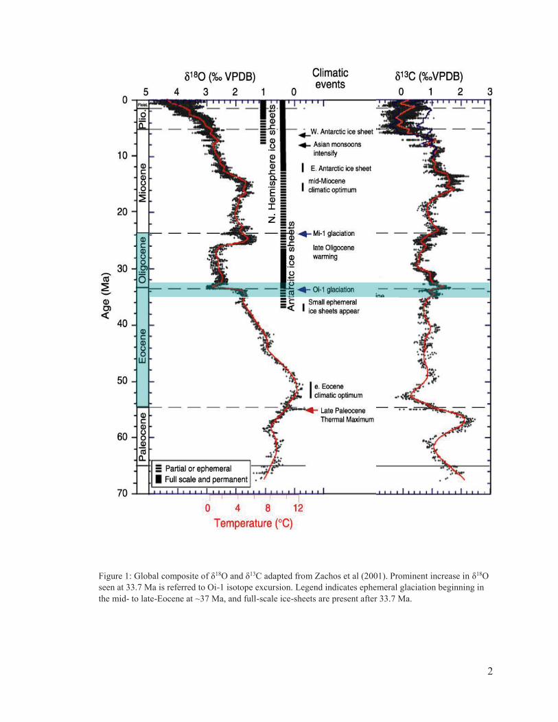
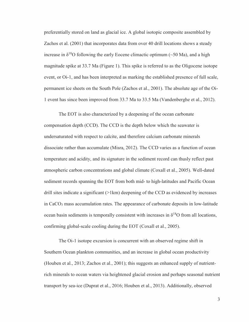
Figure 1: Global composite of δ18O and δ13C adapted from Zachos et al (2001). Prominent increase in δ18O seen at 33.7 Ma is referred to Oi-1 isotope excursion. Legend indicates ephemeral glaciation beginning in the mid- to late-Eocene at ~37 Ma, and full-scale ice-sheets are present after 33.7 Ma.
3
preferentially stored on land as glacial ice. A global isotopic composite assembled by
Zachos et al. (2001) that incorporates data from over 40 drill locations shows a steady
increase in δ18O following the early Eocene climactic optimum (~50 Ma), and a high
magnitude spike at 33.7 Ma (Figure 1). This spike is referred to as the Oligocene isotope
event, or Oi-1, and has been interpreted as marking the established presence of full scale,
permanent ice sheets on the South Pole (Zachos et al., 2001). The absolute age of the Oi-
1 event has since been improved from 33.7 Ma to 33.5 Ma (Vandenberghe et al., 2012).
The EOT is also characterized by a deepening of the ocean carbonate
compensation depth (CCD). The CCD is the depth below which the seawater is
undersaturated with respect to calcite, and therefore calcium carbonate minerals
dissociate rather than accumulate (Misra, 2012). The CCD varies as a function of ocean
temperature and acidity, and its signature in the sediment record can thusly reflect past
atmospheric carbon concentrations and global climate (Coxall et al., 2005). Well-dated
sediment records spanning the EOT from both mid- to high-latitudes and Pacific Ocean
drill sites indicate a significant (>1km) deepening of the CCD as evidenced by increases
in CaCO3 mass accumulation rates. The appearance of carbonate deposits in low-latitude
ocean basin sediments is temporally consistent with increases in δ18O from all locations,
confirming global-scale cooling during the EOT (Coxall et al., 2005).
The Oi-1 isotope excursion is concurrent with an observed regime shift in
Southern Ocean plankton communities, and an increase in global ocean productivity
(Houben et al., 2013; Zachos et al., 2001); this suggests an enhanced supply of nutrient-
rich minerals to ocean waters via heightened glacial erosion and perhaps seasonal nutrient
transport by sea-ice (Duprat et al., 2016; Houben et al., 2013). Additionally, observed

4
shifts in mid-latitude clay mineralogy (Wang et al., 2013) and paleoclimate
reconstructions that indicate low-latitude surface water cooling (Lear et al., 2008) support
the hypothesis that temperature decrease across the EOT was ubiquitous and not confined
to polar regions.
1.1.2 Development of Antarctic Ice Sheets
The growth of Antarctic glaciers across this transition is documented as occurring
in two steps, each lasting ~40 thousand years (kyr), with ~200 kyr between events
(Coxall et al., 2005). The first step, referred to as EOT-1, is characterized as “precursor”
glaciation in response to declining atmospheric CO2 from the high (~1000-2000 ppmv)
concentrations of the Eocene (Miller et al., 2009; Pagani et al., 2005); EOT-1 cooling is
reflected in a slight (~0.6‰) positive δ18O excursion at 33.8 Ma (Katz et al., 2008). The
second step is marked by the larger (~1‰) Oi-1 isotope excursion at 33.5 Ma, and
denotes the presence of an established continental-scale ice sheet with a smaller,
additional cooling component (Passchier et al., 2017; Coxall et al., 2005; Zachos et al.,
2001).
The breadth of details surrounding spatial ice development, sensitivity, and
atmospheric CO2 threshold behavior that are still uncertain warrants continued
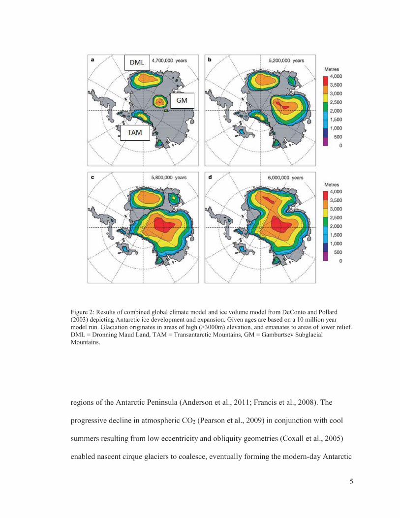
investigation into Antarctica’s ice sheet dynamics during the EOT. Mid- to late-Eocene
glaciation is believed to have nucleated in the high elevations of the Gamburtsev
Mountains (Rose et al., 2013), the Transantarctic Mountains and Dronning Maud Land
regions of East Antarctica (DeConto and Pollard, 2003), and perhaps even mountainous
5
Figure 2: Results of combined global climate model and ice volume model from DeConto and Pollard (2003) depicting Antarctic ice development and expansion. Given ages are based on a 10 million year model run. Glaciation originates in areas of high (>3000m) elevation, and emanates to areas of lower relief. DML = Dronning Maud Land, TAM = Transantarctic Mountains, GM = Gamburtsev Subglacial Mountains.
regions of the Antarctic Peninsula (Anderson et al., 2011; Francis et al., 2008). The
progressive decline in atmospheric CO2 (Pearson et al., 2009) in conjunction with cool
summers resulting from low eccentricity and obliquity geometries (Coxall et al., 2005)
enabled nascent cirque glaciers to coalesce, eventually forming the modern-day Antarctic
6
Ice Sheet (AIS; Figure 2). Recent records compiled from various continental margin
sediment cores and geophysical surveys indicate that large-scale glaciation began on East
Antarctica prior to the EOT-1 isotope excursion (e.g., Gulick et al., 2017, Passchier et al.,
2017, Carter et al., 2016). However, additional records from the Ross Sea embayment of
West Antarctica suggest marine-terminating ice did not stabilize until 32.8 Ma, well after
the transition (Galeotti et al., 2016). Conflicting chronologies imply glacial expansion did
not occur synchronously across the continent, and present a need to improve temporal
constraints of ice development on East and West Antarctica.
Today, the relevance of this research is unequivocal: atmospheric CO2 has
exceeded a level (400 ppm) not seen since 3 Ma, human-induced warming of just 1°C
was already accompanied by 20 cm of global sea level rise (SLR), and research predicts
additional global SLR of 25-30 cm is inevitable over the next 40 years (Naish, 2017).
AIS melting has the potential to significantly contribute to global SLR, and current
satellite measurements show increased melting of Antarctic ice shelves in response to
Southern Ocean warming (Naish, 2017). Models that can accurately project ice sheet
collapse in response to various degrees of warming therefore have immediate
implications for global policy and environmental protection initiatives. To advance
understanding of ice-climate dynamics and improve models for future projections, it is
imperative that research continues reconstructing past ice behavior from times of great
climate variability. This project seeks to contribute to this objective through the multi-
method analysis of well-dated, near-shore Antarctic sediments that span the EOT.
1.2 Study Location
1.2.1 ODP Site 696
7
Site 696 is one of nine sites drilled in the Weddell Sea region during Ocean
Drilling Program (ODP) Leg 113 in 1987 (Shipboard Scientific Party, 1988). In addition
to characterizing the evolution of planktonic productivity and exploring the initiation of
cold Antarctic bottom water in the Weddell Sea sector, a primary objective of Leg 113
was to investigate the temporal development of the modern-day Antarctic ice sheet
(Shipboard Scientific Party, 1988). Located on the southeast margin of the South Orkney
Microcontinent (SOM), Site 696 is an ideal geographic location to examine Antarctica’s
glacial history in the Weddell Sea sector (Figure 3). Continental margin sediments
provide an essentially undisturbed record of paleoenvironmental conditions such as
changes in sediment supply, ocean geochemistry and temperature, and variations in
regional sea level (Passchier et al., 2017; Galeotti et al., 2016). At the poles specifically,
these marginal sediments are useful in reconstructing glacial advance and retreat cycles
and preserving outsized clasts (e.g., Gulick et al., 2017, Carter et al., 2016).
Two holes, 696A and 696B, were drilled at 650 meters water depth. Only 12
cores were recovered from Hole A due to difficulties with the bottom hole assembly.
Hole B was significantly more successful; 62 cores were recovered to a maximum depth
of 645.6 mbsf (Shipboard Scientific Party, 1988). Shipboard scientists divided cores into
lithostratigraphic units based primarily on smear slide analyses and observational
maturity (Shipboard Scientific Party, 1988). Additional characteristics including clay
mineralogy, seismic stratigraphy, and paleomagnetic assignments were observed and
described in detail in the site report (Shipboard Scientific Party, 1988).

8
Figure 3: GeoMap App rendered map showing location of ODP Site 696 (star) in the northwestern Weddell Sea. Recent studies from drill sites in Prydz Bay, the Ross Sea, and Wilkes Land Margin that provide evidence for asynchronous East and West Antarctic ice sheet expansion across the E-O transition are also noted (dots).

9
1.2.2 Weddell Sea Sector Tectonics and Geology
The continent of Antarctica has a rich and complex tectonic history dating back to
the inception of the East Antarctic craton in the Early Archean (Anderson,1999). While
major geologic development of East Antarctica was complete by the early Paleozoic
(Anderson, 1999), West Antarctica’s tectonic history is more recent and complex. West
Antarctica is comprised of five continental blocks (Marie Byrd Land, Thurston Island,
Antarctic Peninsula, Haag Nunataks, and Ellsworth-Whitmore Mountains) that formed
amidst the breakup of Gondwanaland during the Mesozoic era (Lee et al., 2012;
Fitzgerald, 2002). These microplates continued to rotate and translate until reaching their
present configuration approximately 110 Ma (Fitzgerald, 2002). It was this tectonically-
driven rotation that allowed for the opening of the Weddell Sea c. 165 Ma (Fitzgerald,
2002).
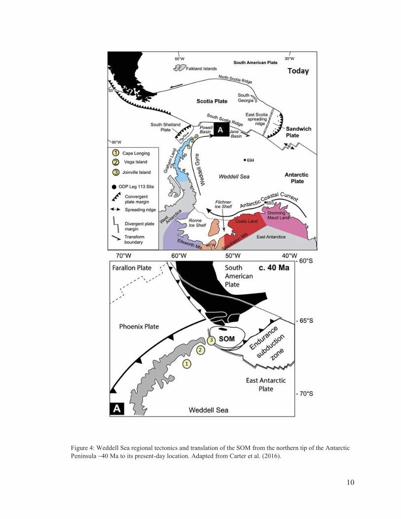
Tectonic activity continued to affect West Antarctica through the mid-Cenozoic;
during the late-Eocene, rifting separated the South American plate and Antarctic
Peninsula microplate, opening the Drake Passage and forming the South Scotia Ridge
(Busetti et al., 2000). It is likely this event separated the SOM from the northern tip of the
Antarctica Peninsula (Eagles and Livermore, 2002); regional extension continued from
~37 to 23 Ma (Eagles and Livermore, 2002), opening the Powell Basin c. 29 Ma and
geographically isolating the SOM (Figure 4). Paleomagnetic reconstructions indicate
during the EOT, sedimentation on the shelf of the SOM would have been restricted to
local sources of the Antarctic Peninsula, or ice-rafted debris (IRD) from distal formations
(Eagles and Livermore, 2002; Busetti et al., 2000).
10
Figure 4: Weddell Sea regional tectonics and translation of the SOM from the northern tip of the Antarctic Peninsula ~40 Ma to its present-day location. Adapted from Carter et al. (2016).
11
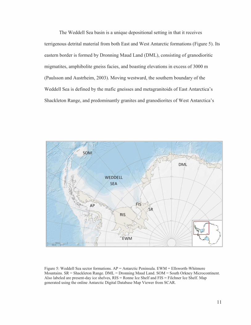
The Weddell Sea basin is a unique depositional setting in that it receives
terrigenous detrital material from both East and West Antarctic formations (Figure 5). Its
eastern border is formed by Dronning Maud Land (DML), consisting of granodioritic
migmatites, amphibolite gneiss facies, and boasting elevations in excess of 3000 m
(Paulsson and Austrheim, 2003). Moving westward, the southern boundary of the
Weddell Sea is defined by the mafic gneisses and metagranitoids of East Antarctica’s
Shackleton Range, and predominantly granites and granodiorites of West Antarctica’s
Figure 5: Weddell Sea sector formations. AP = Antarctic Peninsula. EWM = Ellsworth-Whitmore Mountains. SR = Shackleton Range. DML = Dronning Maud Land. SOM = South Orkney Microcontinent. Also labeled are present-day ice shelves, RIS = Ronne Ice Shelf and FIS = Filchner Ice Shelf. Map generated using the online Antarctic Digital Database Map Viewer from SCAR.
12
Ellsworth-Whitmore Mountains (Will et al., 2010; Vennum and Storey, 1987). These two
regions are geographically separated by the 3500-km long Transantarctic Mountain
(TAM) range (Fitzgerald, 2002), which may also supply lithogenic material to the
Weddell Sea basin. The western border of the Weddell Sea is defined by the Antarctic
Peninsula, which is comprised of upper-Paleozoic to lower-Mesozoic sandstones and
mudstones in the north (Castillo et al., 2014), and both calc-alkaline volcanic rocks and
back-arc basin sedimentary sequences in the south (Vennum and Rowley, 1986).
1.3 Age Model
Much of the ambiguity through the EOT can be attributed to poor core recovery
and lack of certainty in assigning core ages (Houben et al., 2013; Coxall et al., 2005). The
shipboard sequence dating of cores from Site 696 involved bio- and
magnetrostratigraphic methods (Shipboard Scientific Party, 1988). However, poor
preservation of radiolarian and other stratigraphically useful microfossils from much of
the lower (i.e., from ~530 to 645.6 mbsf) cores meant age constraints through the
Paleogene had potential for error.
A recent (2013) study investigated dinoflagellate fossil assemblages in several
cores from the Antarctic margin in order to identify cooling-induced shifts in taxa, and
update existing core ages based on first and last occurrences (Houben et al., 2013).
Researchers examined Hole 696B and were able to improve age constraints by
identifying specific dinocyst appearances and calibrating with well-dated appearances
from other drill sites (Houben et al., 2013, Supplementary Materials [SM]). The study
identified the first occurrence (FO) of Malvinia escutiana, a marker taxon whose FO in a
South Atlantic drill core was correlated to the Oi-1 event (Houben et al., 2011), in Core

13
55R at 569.11 mbsf; this depth was thus assigned an age of 33.6 Myr (Houben et al.,
2013, SM). Additionally, the FO of dinocyst Stoveracysta kakanuiensis, dated to 34.1
Myr, was observed in Core 55R at 571.55 mbsf (Houben et al., 2013, SM).
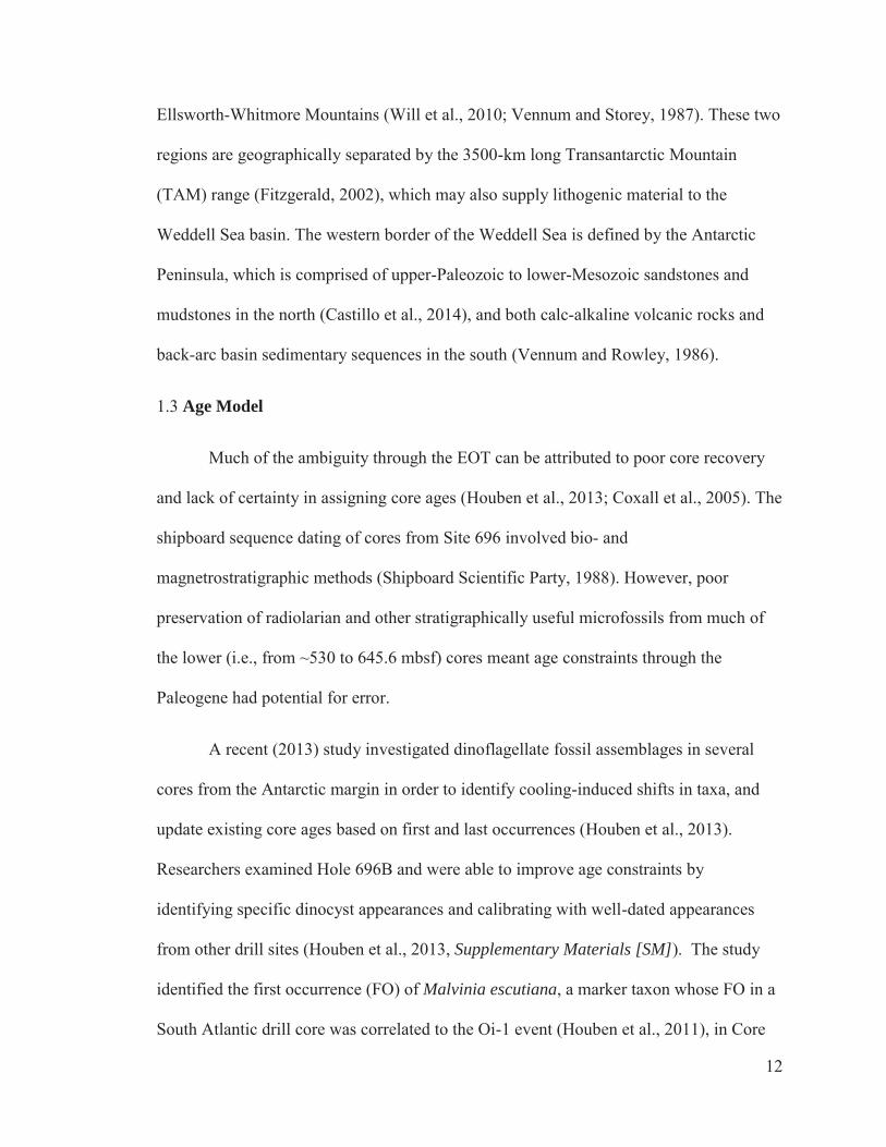
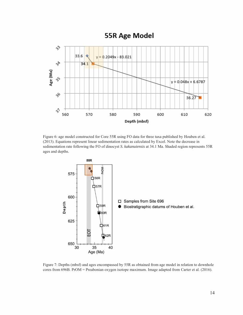
Using these age-to-depth correlations, an age model was constructed for the lower
cores (55R-62R) of 696B (Figure 6). By combining the two relationships detailed above
with a third FO of the calcareous nanofossil Isthmolithus recurves at 616.78 mbsf and
dated to 36.27 Ma (Houben et al., 2013, SM), intermediate sample ages and linear
sedimentation rates were calculated. The stratigraphic placement of S. kakanuiensis
below M. escutiana indicates Core 55R, spanning from 568.7 to 576.1 mbsf, is a high-
recovery core from a sedimentary succession that encompasses the complete EOT at 34
Ma (Figure 7). This study presents a high-resolution analysis of this core, incorporating
geochemical and sedimentological methods, to determine the extent of glacial influence
on sediment deposited at Site 696 across the EOT.
2. METHODOLOGY
2.1 Sedimentological Analysis
The initial analytical method used in this study was laser particle size analysis.
The distribution of particle sizes within a sedimentary sample gives great insight to the
environment during deposition, and any changes to that depositional environment, such
as a new sediment source, shift in weathering regime, or variation in water depth are
often reflected in grain size distribution (e.g., Passchier et al., 2017, Storti and Balsamo,
2010). From October 2016 to February 2017, laser particle size analysis was performed
14
Figure 6: age model constructed for Core 55R using FO data for three taxa published by Houben et al. (2013). Equations represent linear sedimentation rates as calculated by Excel. Note the decrease in sedimentation rate following the FO of dinocyst S. kakanuiensis at 34.1 Ma. Shaded region represents 55R ages and depths.
Figure 7: Depths (mbsf) and ages encompassed by 55R as obtained from age model in relation to downhole cores from 696B. PrOM = Preabonian oxygen isotope maximum. Image adapted from Carter et al. (2016).
15
on 75 samples from Sections 1-5 of Core 55R using the Malvern Mastersizer 2000 at
Montclair State University.
2.1.1 Sample selection
The first step in determining which samples to examine involved applying the age
model to sections 1-5 of Core 55R. Doing so yielded a maximum age of 34.3 Ma at a
corresponding depth of 575.65 mbsf, and a minimum age of 33.52 Ma at corresponding
depth 568.7 mbsf. Each section is divided into samples of two- to three-centimeter
intervals; ages for individual samples were assigned by interpolating between the known
datum published by Houben et al. (2013). As is reflected in the age model for 55R
(Figure 6), the rate of deposition at Site 696 decreased after approximately 34.1 Ma,
above corresponding depth of 571.6 mbsf. This shift is aligned with sample 40-42 cm of
section 55R3. From this depth to the base of 55R5, the time between each sample was
calculated as 2.4 kyr. Above this depth to the top of Core 55R, time between samples
increases to 10.25 kyr.
The samples chosen for analysis were selected with an average of 10 kyr spacing
to ensure sedimentation responses to obliquity and eccentricity cycles could be observed.
Thus, in order to maintain a consistent spacing, this study analyzed every sample from
568.7 mbsf to the top of the core (49 total), and every fourth sample from 568.7 mbsf to
the base of section 5 (26 total). Core sections with corresponding depths and ages are
shown in Figure 8, and a complete listing of all samples is given in the appendix (Table
A.1).

16
Figure 8: Lithologic log of lower cores from Site 696 (adapted from Carter et al., 2016). Core 55R is expanded to show sections used in this study with corresponding depths and ages as calculated from the age model. Shaded regions in 55R denote depths of dinocyst FOs that constrain the EOT. Stars indicate sample depths studied by Carter et al. (2016).
Core 55R
17
2.1.2 Sample preparation
Samples were prepared according to Konert and Vandenberghe (1997). Laser
particle size analysis is restricted to grains less than 2mm in diameter; typically, samples
are sieved to remove coarse-grained material. None of the samples used in this study,
however, exhibited grains in excess of 2mm and therefore no sieving was required.
Approximately 2-3 grams of sample were needed; for those samples with little
cementation, it was possible to manually separate a representative subsample. For others,
subsamples were separated with a hammer, and further disaggregated with a mortar and
pestle using exclusively vertical pressure to avoid breaking grains. Each subsample was
then placed in a 250-mL beaker and ~10 mL of 30% hydrogen peroxide was added to
digest organic material. Millipore water was added to bring total volume to ~50 mL, and
solutions were swirled and left to disaggregate completely. Beakers were then transferred
to hot plates to encourage reactions. None of the samples from 55R reacted with H2O2. 2
mL of 10% HCl was then pipetted into each beaker to remove any carbonate content.
Again, little to no reaction occurred in 55R samples. The solution was then allowed to
boil off until total volume was <50 mL.
The beakers were removed from heat and cooled before components were
transferred to labeled 50 mL polypropylene vials. The vials were transferred to a
centrifuge and spun at 2000 rpm for 30 minutes. The supernatant was discarded, vials
were refilled to 50 mL with Millipore water and shaken to resuspend sediment before
another 30-minute centrifuge. After a second decantation, each specimen was returned to
its original beaker and approximately half a teaspoon of sodium pyrophosphate, a
dispersing agent, was added. Enough Millipore water to bring the solution to 50 mL was
18
added, and beakers were heated just long enough to dissolve the sodium pyrophosphate.
Finally, samples received at least 15 minutes of sonication. Samples that did not
disaggregate after 15 minutes received additional sonic baths in 15-minute intervals until
grains were sufficiently separated for analysis (Table A.2).
Four particularly resistant samples were prepared following the above procedure
but given a sodium hydroxide bath to further encourage disaggregation following
decantation. After the second decantation, vials were filled to 20 mL with Millipore
water, and 5 mL of NaOH was added before placing vials in a water bath between 85-
90ºC for one hour. Vials were then cooled, filled to 50 mL with Millipore water, and run
through the centrifuge at 2000 RMP for another 30 minutes. Following decantation and
two rounds of sonication, both 55R1 90-93 and 55R2 145-147 retained a single clump.
The clumps were manually removed, standard preparation was completed, and particle
size analysis was run with no further complications. A complete list of samples that
received modified preparation for laser particle size analysis is provided in the appendix
(Table A.2).
2.1.3 Data acquisition and processing
Data was collected using the Malvern Mastersizer 2000. The instrument projects
red and blue lasers through a glass cell while a centrifugal pump recirculates sample
suspended in Millipore water (Storti and Balsamo, 2010). Fifty-two sensors measure the
angles of light diffracted by the suspended sediments; the instrument then determines
grain size distribution based on the principle that the angle at which particles diffract light
increases logarithmically as particle size decreases (Storti and Balsamo, 2010). The
instrument was run using the standard operation procedure settings for fine-grained
19
sediments outlined by Sperazza et al. (2004) with a rotor speed of 2000 rpm. A stable
background reading of ~650 mL Millipore water in an 800-mL beaker was used to
measure the background prior to addition of each sample. After the background was
measured, the sample was added to the beaker and the data collection began. Between
samples, clean Millipore water was flushed through the instrument to avoid
contamination, and the probe was thoroughly rinsed of residual sediment. Each sample
was discarded after testing.
Results were exported into an Excel spreadsheet, and grain size percentages were
compiled based on the following classification: grains between .02 and 3.9 microns as
clay, grains between 3.9 and 62.5 microns as silt, and grains between 62.5 and 2000
microns as sand (Wentworth, 1922). The contribution from each of the three size classes
was then calculated in Excel based on total volume within each sample.
2.2 Geochemical Analysis
To supplement sedimentological analysis outlined above, this study also
incorporates examination of bulk geochemistry of samples to further understand
paleoclimate conditions prior to and during deposition, as well as investigate potential
sediment sources. Inductively-coupled plasma mass-spectrometry (ICP-MS) was
performed using a ThermoFischer Scientific iCap-Q instrument at Montclair State
University. A total of four runs was performed to obtain concentrations of trace and rare
earth elements (REE). Inductively-coupled plasma optical emission spectrometry (ICP-
OES) was conducted using a Horiba Jobin-Yvon Ultima instrument for three total runs to
procure major element data.
20
2.2.1 Sample selection
Of the 75 samples analyzed for particle size distribution, 28 samples with mud
fractions (<63μm) in excess of 80% were chosen for geochemical analysis via ICP-MS
and ICP-OES. Samples were selected with a conscious effort to holistically represent
sections 1-5 of Core 55R, with an emphasis on samples surrounding potentially
transitionary deposits as interpreted through particle size data.
2.2.2 Sample preparation
28 samples were ground into a fine, homogenous powder with a mortar and
pestle. Each sample was then weighed to 0.1000g +/- 0.0005g and mixed with 0.4000g
+/- 0.002g of lithium metaborate flux on a weighing paper until homogenous. Weights of
both sample and flux were recorded, and powdered mixtures were transferred to graphite
crucibles. Crucibles were placed into a furnace at 1050º C for 30 minutes, creating a glass
bead. During this time, 50 mL of 7% nitric acid and a magnetic stirbar were added to
Teflon beakers. Once the crucibles were removed from the oven, each bead was
immediately swirled and transferred to a beaker for complete acid digestion. Beakers
were individually placed on a stirring plate to aid the bead’s dissolution; once each bead
was completely dissolved, the solution was funneled through filter paper into a 60 mL
Nalgene bottle. This sample preparation was carried out according to Murray et al. (2000)
and yielded master solutions with a 500x dilution factor.
Murray et al. (2000) recommend a 4000x dilution factor for analysis on the ICP-
OES. This solution was created by pipetting 6.5 mL of the 500x master solution into new
60 mL Nalgene bottles. Then, 50 mL of 2% nitric acid was measured with a volumetric
21
flask and poured into the bottle. These 4000x solutions were stored in a refrigerator until
ready for analysis. Instrumental sensitivity of ICP-MS makes it an ideal method for
measuring trace and REE in bulk rock samples (Tamura et al., 2015); samples therefore
required further dilution to 10,000x prior to ICP-MS analysis. This was done by pipetting
0.5 mL of each master solution into a test tube, and then adding 9.5 mL of 2% nitric acid
for an additional dilution factor of 20x.
2.2.3 Data acquisition and processing
ICP-MS
Test tubes containing 10,000x diluted samples were racked and entered by sample
ID according to rack placement into the iCap-Q software. The rack also included three
blanks of only lithium metaborate flux and 12 United States Geological Survey (USGS)
standards, prepared and diluted identical to samples. The instrument collected readings of
a drift solution after every fourth sample; raw data was then exported into an Excel
spreadsheet, and corrected for instrument drift and blank measurements. Ten of the 12
USGS standards with igneous compositions were used to derive calibration lines for each
element. To assess accuracy of these calibrations, two sedimentary USGS rock powders
were used as secondary standards.
A complete sample analysis consists of three runs; an initial run was conducted in
July 2017, but technical difficulties with the instrument prevented completion of the final
two runs. From this first run, exported data revealed precise calibrations for all minor
elements. In October 2017, a new set of dilutions from the master solutions was prepared
and three runs were successfully completed. Calibrations for rare earth and trace elements
22
were precise with the exception of Co. Data from all four runs was averaged and used in
geochemical analysis, except Co, where only data procured during the initial run is used.
Average trace and REE concentrations used in analysis are given in Tables A.3 and A.4,
respectively.
ICP-OES
Samples were transferred from the 4000x dilution bottles into racked test tubes,
whose corresponding sample IDs were input to the instrument software according to rack
placement. Included in the rack were three blank solutions and 12 USGS standards, also
with a dilution factor of 4000x, and drift measurements were taken after every fourth
sample. Data processing in Excel revealed major element calibrations against USGS
standards were precise in all three runs, except for element Mn for standard QLO-1. The
calibration plot exhibited one outlying data point for the QLO-1 standard, which was
removed from averages. Averaged major element concentrations are provided in Table
A.5.
2.3 Paleoenvironmental Proxies and Ratios
2.3.1. Ice-Rafted Debris Mass Accumulation Rate
Major element results from the ICP-OES, in conjunction with particle size data,
have been used to calculate the ice-rafted debris mass accumulation rate (IRD MAR).
Fluctuations in IRD MAR can be indicative of both a change in a depositional
environment’s energy, and/or a shift in the supply of sediment to a sink. IRD MAR can
also serve as a proxy to gauge sea-ice abundance (Hebbeln, 2000). Values were
23
calculated using the following equation from Krissek (1998):
(1)
where IRD is the volume fraction of grains >125 microns (determined from laser particle
size data), LSR is the linear sedimentation rate (cm/kyr; obtained from the 55R age
model, Figure 6), DBD is the dry bulk density (g/cm3), and TERR is the terrigenous
fraction. DBD was calculated according to Grützner (2003) using wet bulk density
obtained from the JANUS database (2017). The terrigenous fraction is given by:
(2)
The carbonate percent was determined to be negligible on the grounds that (i) samples
exhibited little to no reaction to hydrochloric acid during particle size analysis
preparation and (ii) the smear slide analysis included in the Site 696 core report indicates
carbonate is absent in 55R (Shipboard Scientific Party, 1988). The biogenic silica percent
was calculated as excess silica according to Böning et al. (2005), where:
(3)
24
Oxide sample percents were taken from ICP-OES data, and the lithogenic fraction was
obtained from averaging published geochemical data from mudstones of the Hope Bay
and Cape Legoupil Formations of the local Trinity Peninsula Group (Castillo et al., 2014,
SM).
2.3.2. Chemical Index of Alteration
Major element data were also used to calculate the chemical index of alteration
(CIA). CIA is a weathering proxy useful for differentiating between chemical and
physical weathering regimes by examining the molar ratio of mobile cations commonly
released in warm environments, and is calculated according to Nesbitt and Young (1982)
as:
(4)
The calculations use molar weights of each oxide as determined from the normalized
weight percents.
2.3.3 Elemental Enrichments
Interpreting trends and patterns in trace, rare earth, and major element
concentration throughout the core is another analytical approach to better understand
terrestrial weathering regimes and the nature of sediment origin. To begin, trace and rare
earth elemental averages in ppm were calculated for each sample including data from all
four ICP-MS runs. Those averages were then normalized to canonical values of the
Upper Continental Crust (UCC) and average chondrite values for trace and REE,
25
respectively (McLennan, 2001; Nakamura, 1974). Results are displayed on logarithmic
scales to better accentuate interesting geochemical deviations.
2.3.4 Provenance Constraints
The ability to correlate geochemical data to potential source rocks has
implications for reconstructing ice growth in the Weddell Sea sector. To do so, this study
analyzes fluctuations, ratios, and trends in trace and REE to observe possible changes in
source material. Additionally, differentiating between felsic and mafic source rocks and
evaluating agreement between samples and a variety of Antarctic formations will shed
light on the regional glacial expansion within the Weddell Sea sector during the EOT.
To determine if sediment originated from one or several sources, a plot showing
Al2O3 vs. TiO2 and Sc vs. TiO2 was constructed. Concentrations of these major and trace
elements are not significantly altered by processes like weathering, sediment sorting, or
diagenesis, and are therefore useful in provenance studies (Sheldon and Tabor, 2009;
McLennan, 2001). Fluctuations in these ratios throughout the core would suggest
multiple sources. Th/Sc was plotted against Zr/Cr to characterize the felsic-mafic nature
of 55R sediments. Standards from USGS samples, the North American Shale Composite
(NASC), and Mid-Ocean Ridge Basalt (MORB) were included for reference.
To further examine the origin of core sediments, a Th/U vs. Th plot (McLennan
eta l., 1993) was made to compare 55R data with different crust/mantle sources and
tectonic settings. Finally, 55R data were plotted with published averages from formations
in the Weddell Sea sector of Antarctica, including the northern and southern Antarctic
26
Peninsula, Dronning Maud Land, the Shackleton Range, and Ellsworth-Whitmore
Mountains, to evaluate geochemical similarities.
3. RESULTS
3.1 Particle Size Distributions
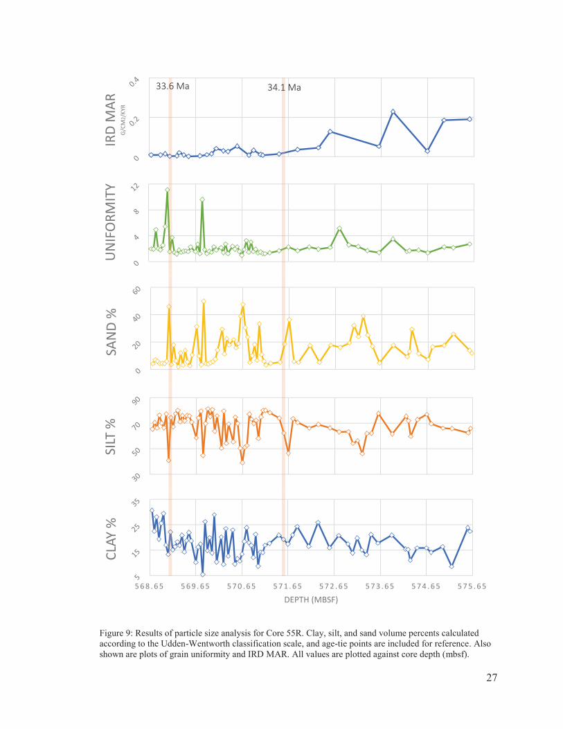
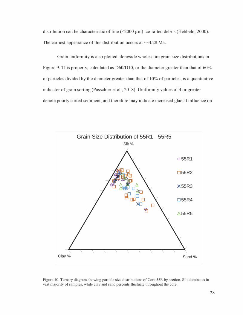
Laser particle size analysis shows that the sediments sampled in sections 1-5 of
Core 55R are consistently dominated by silt, and contributing volume percent of clay and
sand fluctuate (Figure 9). While distributions of individual samples exhibit greater
variance, comparing the averages of each section yield clay percents ranging from 15.9
and 19.9, silt percents between 62.1 and 70.0, and sand percents between 10.0 and 20.4.
There is an overall trend of increasing silt contribution upcore; this becomes evident
when samples are plotted by section on a ternary diagram (Figure 10). The ternary
projection also highlights individual samples whose sand contributions reach 40-50%.
Additionally, the average volume contribution from clay-sized particles in 55R decreases
slightly upcore.
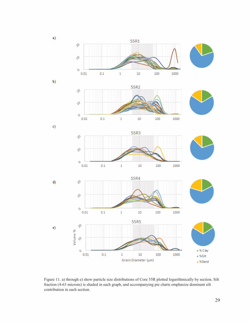
Grain size distributions of individual samples are shown by section in Figure 11
accompanied by their average percent sand, silt, and clay. Here, the slight trend of
increasing silt percent and decreasing clay percent upcore becomes more apparent. Each
section can be characterized as exhibiting several bi-modal distributions that fall within
the silt-sized range, with lesser and roughly equal contributions from clay and sand sized
grains. Interestingly, each section except 55R3 exhibits at least one sample whose
distribution is dominated by silt, but features a small, coarse-grained “tail”; this
27
Figure 9: Results of particle size analysis for Core 55R. Clay, silt, and sand volume percents calculated according to the Udden-Wentworth classification scale, and age-tie points are included for reference. Also shown are plots of grain uniformity and IRD MAR. All values are plotted against core depth (mbsf).
5 6 8 . 6 5 5 6 9 . 6 5 5 7 0 . 6 5 5 7 1 . 6 5 5 7 2 . 6 5 5 7 3 . 6 5 5 7 4 . 6 5 5 7 5 . 6 5
CLAY
%
DEPTH (MBSF)
SILT
%SA
ND %
UNIF
ORM
ITY
IRD
MAR
G/
CM2/
KYR
33.6 Ma 34.1 Ma
28
distribution can be characteristic of fine (<2000 μm) ice-rafted debris (Hebbeln, 2000).
The earliest appearance of this distribution occurs at ~34.28 Ma.
Grain uniformity is also plotted alongside whole-core grain size distributions in
Figure 9. This property, calculated as D60/D10, or the diameter greater than that of 60%
of particles divided by the diameter greater than that of 10% of particles, is a quantitative
indicator of grain sorting (Passchier et al., 2018). Uniformity values of 4 or greater
denote poorly sorted sediment, and therefore may indicate increased glacial influence on
Figure 10. Ternary diagram showing particle size distributions of Core 55R by section. Silt dominates in vast majority of samples, while clay and sand percents fluctuate throughout the core.
Grain Size Distribution of 55R1 - 55R5
55R1
55R2
55R3
55R4
55R5
Silt %
Sand %Clay %
29
Figure 11. a) through e) show particle size distributions of Core 55R plotted logarithmically by section. Silt fraction (4-63 microns) is shaded in each graph, and accompanying pie charts emphasize dominant silt contribution in each section.

30
sediment erosion. Below 572.75 mbsf (34.17 Ma), sediment remains well-sorted with an
average uniformity value of 2.1, despite fluctuations in clay and sand percents. Upcore
grain uniformity then begins to exhibit greater variation, and the two most significant
peaks with values U>8 align with increases in sand percent above 569.8 mbsf (33.74
Ma).
3.2 Geochemistry
3.2.1 Paleoenvironmental Proxies
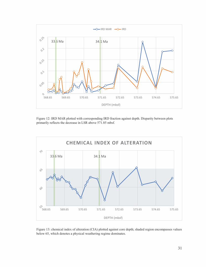
IRD MAR was calculated according to Equation 1, and combines both
sedimentological and geochemical data to help characterize paleoenvironment. Results
were plotted with units of g/cm2/kyr against core depth (Figure 9). Prior to ~34.14 Ma
(572.3 mbsf), IRD MAR fluctuates between values as high as 0.22 and as low as 0.02
g/cm2/kyr. Upcore, IRD MAR remains comparatively low, with values of 0.05 g/cm2/kyr
or below. As noted in the equation, the linear sedimentation rate is factored into the
calculation. Prior to 34.1 Ma, LSR is 2.025 cm/kyr. Sedimentation then drops over 75%
to 0.491 cm/kyr. Figure 12 shows IRD MAR plotted against IRD, another variable in the
calculation. The relationship seen here suggests IRD MAR values are significantly
influenced by the differences in LSR, as numerous samples upcore of the sedimentation
shift display comparable contributions from grains >125 μm. Values for DBD and TERR
do not exhibit notable variation throughout 55R.
The CIA was calculated according to Equation 4 and plotted against core depth
(Figure 13). Values remain below 65 throughout and show a core average of 61. Two
31
Figure 12: IRD MAR plotted with corresponding IRD fraction against depth. Disparity between plots primarily reflects the decrease in LSR above 571.85 mbsf.
Figure 13: chemical index of alteration (CIA) plotted against core depth; shaded region encompasses values below 65, which denotes a physical weathering regime dominates.
568.65 569.65 570.65 571.65 572.65 573.65 574.65 575.65
DEPTH (mbsf)
CHEMICAL INDEX OF ALTERATION
568.65 569.65 570.65 571.65 572.65 573.65 574.65 575.65
DEPTH (mbsf)
IRD MAR IRD
34.1 Ma33.6 Ma.6 .1
34.1 Ma 33.6 Ma
32
notable drops to 56 and 57 occur at 571.85 and 570.55 mbsf, respectively. All values
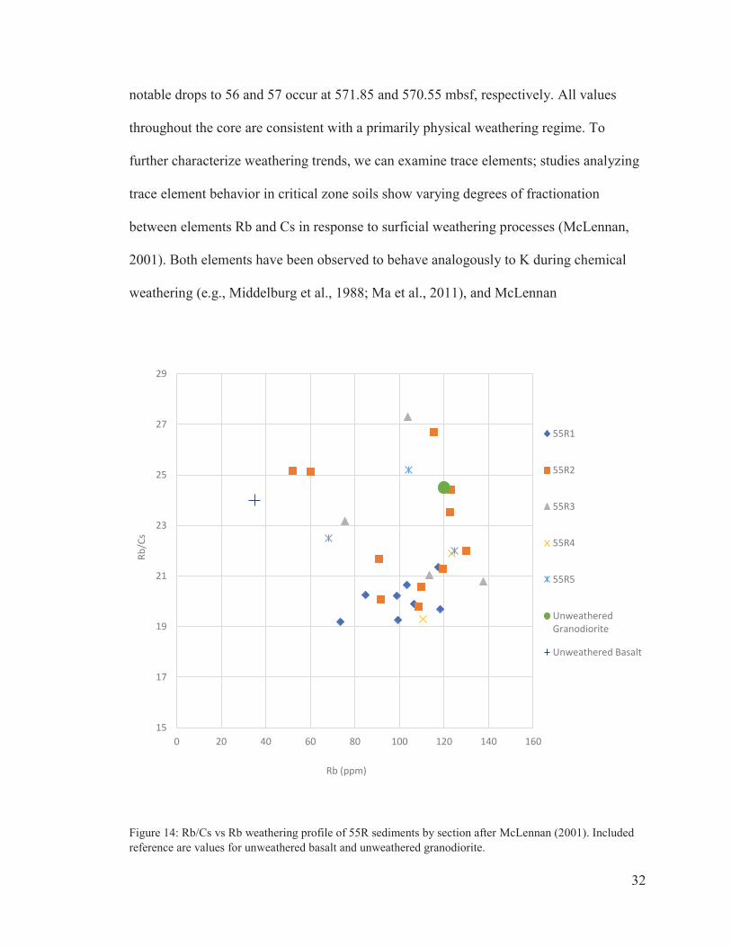
throughout the core are consistent with a primarily physical weathering regime. To
further characterize weathering trends, we can examine trace elements; studies analyzing
trace element behavior in critical zone soils show varying degrees of fractionation
between elements Rb and Cs in response to surficial weathering processes (McLennan,
2001). Both elements have been observed to behave analogously to K during chemical
weathering (e.g., Middelburg et al., 1988; Ma et al., 2011), and McLennan
Figure 14: Rb/Cs vs Rb weathering profile of 55R sediments by section after McLennan (2001). Included reference are values for unweathered basalt and unweathered granodiorite.
15
17
19
21
23
25
27
29
0 20 40 60 80 100 120 140 160
Rb/C
s
Rb (ppm)
55R1
55R2
55R3
55R4
55R5
UnweatheredGranodiorite
Unweathered Basalt
33
(2001) asserts upper crust Rb/Cs ratios are decreased in residual sediment as Cs
exchanges onto clay minerals when interacting with natural waters. 55R values of Rb/Cs
vs. Rb show varying degrees of fractionation with respect to Rb (Figure 14). Samples
from section 1 display the least amount of fractionation (Rb/Cs values from 19.2-21.3),
while section 2 samples show the greatest variation (19.7-26.7).
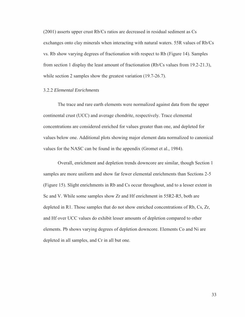
3.2.2 Elemental Enrichments
The trace and rare earth elements were normalized against data from the upper
continental crust (UCC) and average chondrite, respectively. Trace elemental
concentrations are considered enriched for values greater than one, and depleted for
values below one. Additional plots showing major element data normalized to canonical
values for the NASC can be found in the appendix (Gromet et al., 1984).
Overall, enrichment and depletion trends downcore are similar, though Section 1
samples are more uniform and show far fewer elemental enrichments than Sections 2-5
(Figure 15). Slight enrichments in Rb and Cs occur throughout, and to a lesser extent in
Sc and V. While some samples show Zr and Hf enrichment in 55R2-R5, both are
depleted in R1. Those samples that do not show enriched concentrations of Rb, Cs, Zr,
and Hf over UCC values do exhibit lesser amounts of depletion compared to other
elements. Pb shows varying degrees of depletion downcore. Elements Co and Ni are
depleted in all samples, and Cr in all but one.
34
Figure 15. Trace element concentrations of 55R by section, normalized to canonical values of upper continental crust (McLennan, 2001). ^Co denotes only one measurement used in calculations. All other values are based on averages of four instrument runs.
Sc V Cr ^Co Ni Rb Zr Nb Cs Hf Ta Pb Th
SAM
PLE/
UCC
55R1
Sc V Cr ^Co Ni Rb Zr Nb Cs Hf Ta Pb Th
SAM
PLE/
UCC
55R2
Sc V Cr ^Co Ni Rb Zr Nb Cs Hf Ta Pb Th
SAM
PLE/
UCC
55R3-5
35
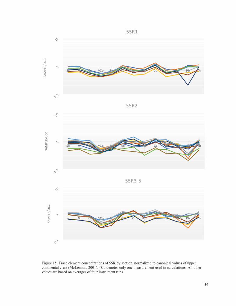
Figure 16: Chondrite-normalized REE concentrations for Core 55R separated by section. Values from Nakamura (1974).
La Ce Pr Nd Sm Eu Gd Tb Dy Ho Er Tm Yb Lu
Sam
ple/
Chon
drite
55R1
La Ce Pr Nd Sm Eu Gd Tb Dy Ho Er Tm Yb Lu
Sam
ple/
Chon
drite
55R2
La Ce Pr Nd Sm Eu Gd Tb Dy Ho Er Tm Yb Lu
Sam
ple/
Chon
drite
55R3-5
36
The chondrite-normalized REE plot almost identically downcore (Figure 16).
Most notable is the prominent negative Eu anomaly exhibited by all samples. This
anomaly, denoted Eu/Eu*, is calculated as
(6)
where subscript N denotes normalized values (McLennan, 2001). Enrichment of the light
REEs (La – Sm; LREE) increases slightly downcore while very minor enrichments of
heavy HREEs (Gd – Lu; HREE) remain consistent. The exception here is Yb,
demonstrating a greater degree of enrichment over other HREEs in all samples, which
show consistently flat (i.e., GdN/YbN = 1.0 to 2.0) patterns (McLennan et al., 1993).
3.2.3 Provenance Constraints
To determine whether sediment deposited at Site 696 in this core interval came
from one or multiple sources, it is useful to examine immobile, or conservative, elemental
ratios. These elements are least fractionated by weathering processes and diagenesis and
thus retain the geochemical signature of their parent rock (Piper & Bau, 2013;
McLennan, 2001). Major elemental ratio Ti/Al has been used to confirm similar
provenance in paleosols, despite variations in weathering on parent material (Sheldon and
Tabor, 2009). Figure 17 shows Al2O3 plotted against TiO2, supplemented by immobile
Sc. Both elements show a linear decrease in concentration with respect to Ti; the absence
of obvious groupings suggests 55R sediments are of a common origin (Figure 17).
37
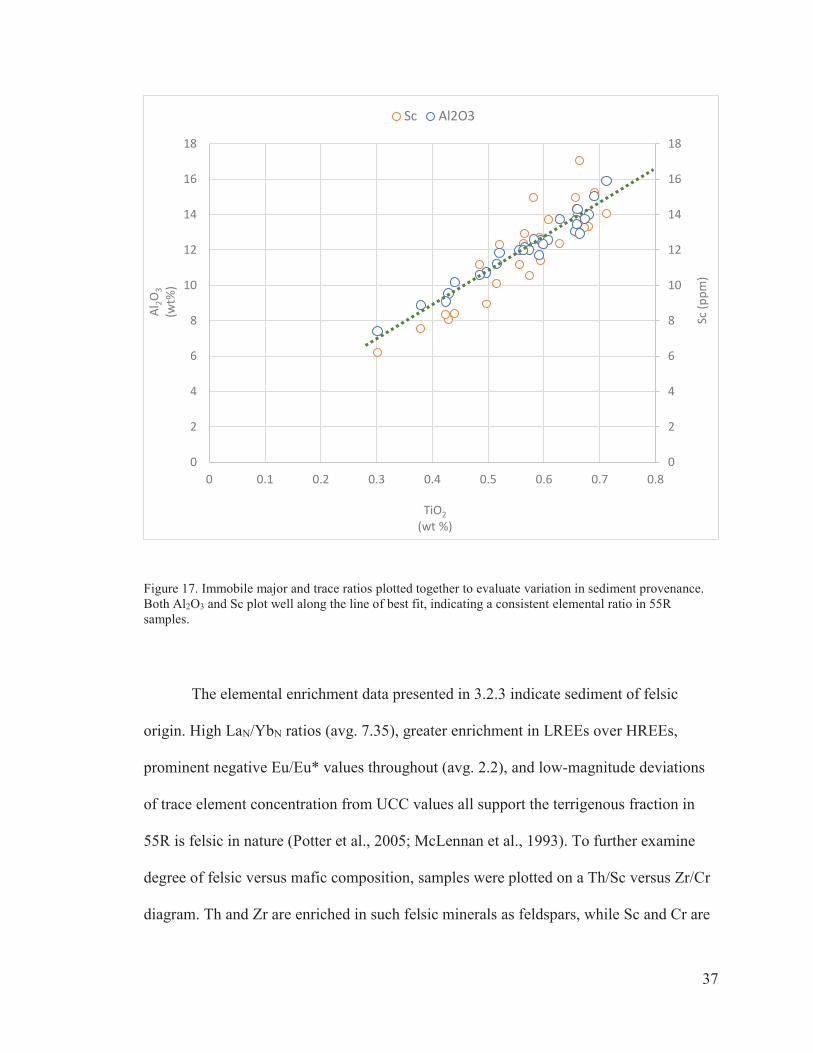
Figure 17. Immobile major and trace ratios plotted together to evaluate variation in sediment provenance. Both Al2O3 and Sc plot well along the line of best fit, indicating a consistent elemental ratio in 55R samples.
The elemental enrichment data presented in 3.2.3 indicate sediment of felsic
origin. High LaN/YbN ratios (avg. 7.35), greater enrichment in LREEs over HREEs,
prominent negative Eu/Eu* values throughout (avg. 2.2), and low-magnitude deviations
of trace element concentration from UCC values all support the terrigenous fraction in
55R is felsic in nature (Potter et al., 2005; McLennan et al., 1993). To further examine
degree of felsic versus mafic composition, samples were plotted on a Th/Sc versus Zr/Cr
diagram. Th and Zr are enriched in such felsic minerals as feldspars, while Sc and Cr are
0
2
4
6
8
10
12
14
16
18
0
2
4
6
8
10
12
14
16
18
0 0.1 0.2 0.3 0.4 0.5 0.6 0.7 0.8
Sc (p
pm)
Al2O
3(w
t%)
TiO2(wt %)
Sc Al2O3

38
prevalent in mafic minerals including olivines and amphiboles (Potter et al., 2005).
Additionally, the low solubility of these elements makes them useful indicators in
sediment provenance studies (Potter et al., 2005). For comparison, averages from
Figure 18: Th/Sc versus Zr/Cr plot featuring 55R samples in relation to USGS standards and additional composites. Composite data from Gromet et al., 1984; Pearce, 1983; Wedepohl, K.H., 1985. After McLennan et al., 1993.
0.001
0.01
0.1
1
10
100
0.1 1 10 100
Th/S
c
Zr/Cr
55R
NASC
MORB
Basalt
Granite
Andesite
Granodiorite
Dolerite
Lower Crust
Felsic
Mafic
39
various lithologic composites and USGS standards were plotted as well (Figure 18). 55R
samples plot well with each other, confirming a similar composition. This projection does
not support mafic parent rocks like dolerite and basalt, and shows 55R contains less felsic
material than standard granite and granodiorite. samples most closely align with values of
the NASC, and to a lesser extent, lower crust.
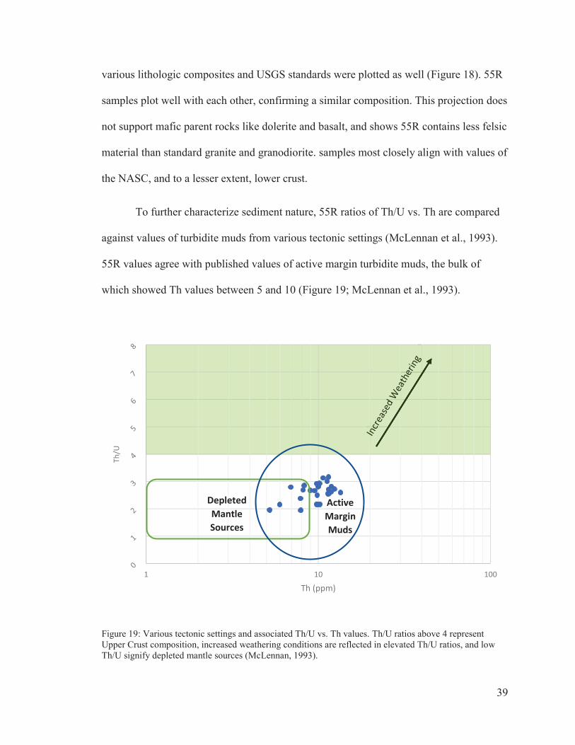
To further characterize sediment nature, 55R ratios of Th/U vs. Th are compared
against values of turbidite muds from various tectonic settings (McLennan et al., 1993).
55R values agree with published values of active margin turbidite muds, the bulk of
which showed Th values between 5 and 10 (Figure 19; McLennan et al., 1993).
Figure 19: Various tectonic settings and associated Th/U vs. Th values. Th/U ratios above 4 represent Upper Crust composition, increased weathering conditions are reflected in elevated Th/U ratios, and low Th/U signify depleted mantle sources (McLennan, 1993).
1 10 100
Th/U
Th (ppm)
Depleted Mantle Sources
Active Margin Muds
40
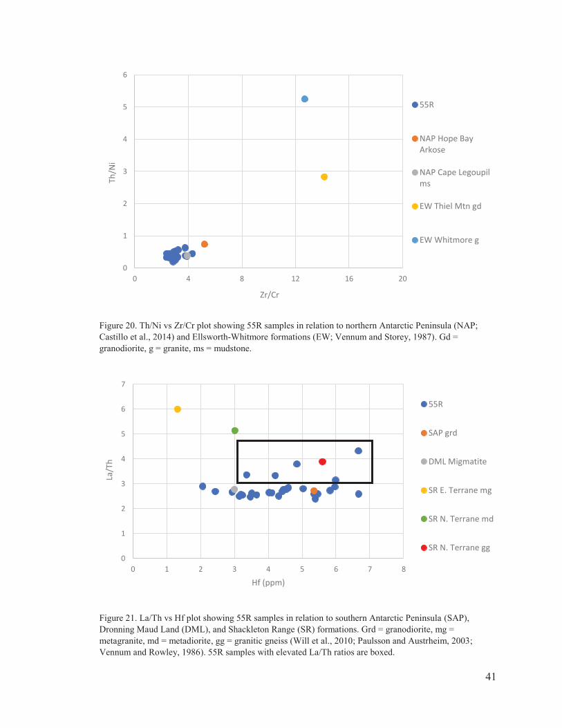
Finally, provenance constraints were applied by comparing 55R data with
published ratios from East and West Antarctic formations in the Weddell Sea sector. Two
plots were constructed based on trace and REE data available. Figure 20 shows Th/Ni
plotted against Zr/Cr. There is strong agreement between 55R samples and both the Hope
Bay and Cape Legoupil formations of the northern Antarctic Peninsula, which consist of
nearly unaltered mudstones and sandstones (Castillo et al., 2014). Samples from 55R do
not plot well with either the granodiorite or the granite from the Ellsworth-Whitmore
Mountains of West Antarctica (Vennum and Storey, 1987), suggesting 55R is more
intermediate in composition than surrounding granitic suites.
A plot of La/Th against Hf reveals 55R sediments do not geochemically resemble
the metadiorites or metagranites from the Shackleton Range of East Antarctica (Figure
21, after Floyd and Leveridge, 1987). 55R samples do, however, plot reasonably well
with granitic gneisses from the North Terrane region of the Shackleton Range and
homogenous granodioritic migmatites from Dronning Maud Land. Again, sample ratios
agree most notably with more local sources from the Antarctic Peninsula; the Latady and
Mount Poster Formations of the Southern peninsula are characterized as upper-crustal
granitoids and granodiorites (Vennum and Rowley, 1986). These agreements support a
felsic origin for 55R samples. Samples show a range of Hf values between 2 and 7 ppm,
and La/Th ratios are quite consistent, except for four samples with elevated La
concentrations (Figure 21).
41
Figure 20. Th/Ni vs Zr/Cr plot showing 55R samples in relation to northern Antarctic Peninsula (NAP; Castillo et al., 2014) and Ellsworth-Whitmore formations (EW; Vennum and Storey, 1987). Gd = granodiorite, g = granite, ms = mudstone.
Figure 21. La/Th vs Hf plot showing 55R samples in relation to southern Antarctic Peninsula (SAP), Dronning Maud Land (DML), and Shackleton Range (SR) formations. Grd = granodiorite, mg = metagranite, md = metadiorite, gg = granitic gneiss (Will et al., 2010; Paulsson and Austrheim, 2003; Vennum and Rowley, 1986). 55R samples with elevated La/Th ratios are boxed.
0
1
2
3
4
5
6
0 4 8 12 16 20
Th/N
i
Zr/Cr
55R
NAP Hope BayArkose
NAP Cape Legoupilms
EW Thiel Mtn gd
EW Whitmore g
0
1
2
3
4
5
6
7
0 1 2 3 4 5 6 7 8
La/T
h
Hf (ppm)
55R
SAP grd
DML Migmatite
SR E. Terrane mg
SR N. Terrane md
SR N. Terrane gg
42
4. DISCUSSION
4.1 Paleoclimate Conditions
4.1.1 Depositional Environment
Results from the laser particle size analysis can be interpreted to infer plausible
environmental settings during time of sediment deposition. The pie charts shown in
Figure 11 demonstrate relatively consistent grain size distributions throughout all sections
of 55R. This suggests that from 34.3 Ma to 33.52 Ma, the shelf of the SOM was not
subject to major changes in relative sea level (RSL). Low clay percent, a reasonable sand
fraction, and the presence of glauconite downhole (57R) indicate a shallow water
environment; indeed, reconstructions suggest paleodepth of ~550 m (Wei and Wise,
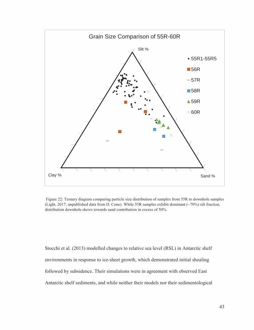
1990). However, when 55R samples are plotted on a ternary diagram with downhole
samples dated up to 36.63 Ma, a new trend emerges (Figure 22). This shift in distribution
can be characterized as a fining upward sequence, transitioning from predominantly sand-
and silt-size grains to majority silt-sized grains with roughly equal, lesser percent
contributions from silt- and clay-sized grains.
Fining upward sedimentary sequences generally indicate a transgressive
environment, where the increase in water depth allows for the settling of finer particles
(Boggs, Jr., 2011). However, research demonstrating eustatic sea level fall (Houben et
al., 2012; Katz et al., 2008) combined with evidence for significant ice development
during the EOT do not support this interpretation. Relative SLR on the SOM shelf may
therefore be explained by crustal subsidence in response to regional glacial expansion;
43
Figure 22: Ternary diagram comparing particle size distribution of samples from 55R to downhole samples (Light, 2017; unpublished data from D. Cone). While 55R samples exhibit dominant (~70%) silt fraction, distribution downhole skews towards sand contribution in excess of 50%.
Stocchi et al. (2013) modelled changes to relative sea level (RSL) in Antarctic shelf
environments in response to ice-sheet growth, which demonstrated initial shoaling
followed by subsidence. Their simulations were in agreement with observed East
Antarctic shelf sediments, and while neither their models nor their sedimentological
Grain Size Comparison of 55R-60R
55R1-55R5
56R
57R
58R
59R
60R
Silt %
Sand %Clay %
44
analysis investigated EOT conditions in the Weddell Sea sector, similar processes may
have occurred proximal to Site 696 (Stocchi et al., 2013).
Because of the timescale represented by this sedimentary sequence, change in
RSL may better be explained by regional tectonic expansion. Initial rifting of the SOM
from the Antarctic Peninsula is thought to have begun in the late Eocene (Eagles and
Livermore, 2002; King and Barker, 1988). Particle size data shows a permanent decline
in significant (42-63%) sand contribution following ~34.9 Ma, which is temporally
consistent with initial stages of SOM rifting beginning at ~37 Ma (King and Barker,
1988). Crustal subsidence associated with regional tectonism is therefore another
plausible driving factor behind increasing water depth on the SOM margin from the late
Eocene to early Oligocene (Livermore et al., 2005).
4.1.2 Weathering Regime
Following the Paleogene-Eocene Thermal Maximum (PETM) at 55.8 Ma
(Vandenburghe et al., 2012), chemical weathering was prevalent across the Antarctic
continent, as evidenced by high mean atmospheric temperatures (MAT) and precipitation
from paleoclimate reconstructions (e.g., Light, 2017, Passchier et al., 2017, Feakins et al.,
2014) and kaolinitic clay assemblages from East and West Antarctic margins (Houben et
al., 2013; Shipboard Scientific Party, 1988). One of the strongest pieces of evidence for
the climate transition at 34 Ma is observed shifts in clay mineralogy, in Antarctica and
elsewhere (Houben et al., 2013; Wang et al., 2013). Where kaolinite and smectite are
indicative of chemical weathering and extensive breakdown of feldspar minerals, illite
and chlorite signify a physical weathering regime (Robert and Maillot, 1990).
45
The Site Report for 696 indicates clay mineralogy in 55R is dominated by
smectite (~70%), with ~10% chlorite and 20% illite (Robert and Maillot, 1990). There is
a noticeable increase in illite and to a lesser extent, chlorite minerals in 55R as compared
to 696 cores of the mid- to late-Eocene (Robert and Maillot, 1990). The preservation of
these minerals in conjunction with consistently glacial CIA values reflect a more arid,
cooler climate where terrigenous weathering is less governed by chemical processes. The
coincidence of 55R’s lowest CIA value with the initial drop in LSR at ~34.1 Ma provides
further evidence for increasing terrestrial climate deterioration.
This steady glacial weathering signature throughout 55R agrees with other climate
reconstruction studies for the Antarctic Peninsula, which indicate decreasing
temperatures and precipitation rates prior to the EOT (e.g., Feakins et al., 2014, Anderson
et al., 2011). Weathering conditions in the northwestern Weddell Sea sector are also
consistent with those reconstructed for the Prydz Bay region, where shelf sediments
begin to reflect glacial CIA values as early as ~34.2 Ma (Passchier et al., 2017). Earliest
Oligocene sediments from the Wilkes Land Margin of East Antarctica also exhibit CIA
values within the glacial range (Light, 2017), confirming large-scale regional cooling
across the EOT.
In the Ross Sea sector, however, an observed shift in clay mineralogy denotes the
transition to a dryer, cooler environment did not occur in West Antarctic until 32.8 Ma
(Galeotti et al., 2016). It has been suggested West Antarctica maintained a warmer
climate longer than did East Antarctica because it was affected by southward flowing
surface currents (Robert and Maillot, 1990). CIAs calculated from 55R suggest regional
cooling and the shift from chemical to physical weathering in the Weddell Sea sector
46
occurred earlier than 34.3 Ma. This also indicates climatic conditions favoring glacial
expansion dominated in this region earlier than other studies show, therefore offering
support for asynchronous climate deterioration and associated ice sheet development
across the Antarctic continent.
4.1.3 Particle Size Distributions
The combination of significant (~70%) silt contribution to 55R samples with
corresponding CIA values consistently within the glacial range indicates sediment
delivered to the SOM margin maintains a glaciogenic signature. Under a warm, wet,
climate where chemical weathering prevails, silt-sized minerals are likely to break down
to clay minerals (Thiry, 2000). The preservation of the silt fraction in 55R samples
indicates environmental conditions were not conducive for pedogenic completion, as is
confirmed by CIA values below 65. Passchier et al. (2017) assert detrital material
associated with glacial erosion (i.e., glacial rock flour) is found predominately in the silt
fraction. Low clay percents throughout the core suggest a relatively shallow depositional
environment and strong physical weathering conditions.
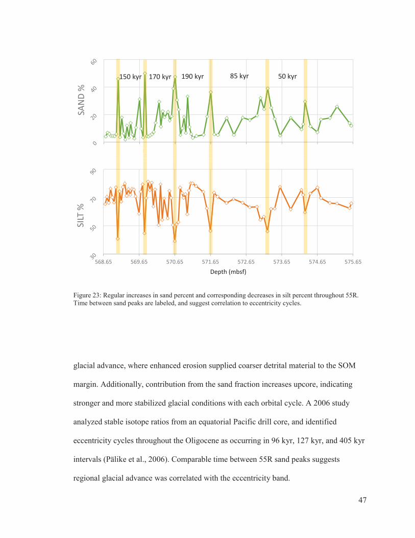
Eccentricity and obliquity geometries yielded cooler summers and provided
environmental conditions conducive for high latitude ice growth during the EOT (Coxall
et al., 2005), and orbitally-paced glacial advance and retreat cycles during this transition
have been recognized in East and West Antarctic margin sediments (e.g., Passchier et al.,
2017, Galeotti et al., 2016). 55R exhibits regular fluctuations in sand percent, with
spacings every ~60 kyr prior to 34.1 Ma, and every ~170 kyr after (Figure 23). This
implies 55R captured local, land terminating glacial responses to changes in orbital
configurations; peaks in sand percent are interpreted as representing periods of regional
47
Figure 23: Regular increases in sand percent and corresponding decreases in silt percent throughout 55R. Time between sand peaks are labeled, and suggest correlation to eccentricity cycles.
glacial advance, where enhanced erosion supplied coarser detrital material to the SOM
margin. Additionally, contribution from the sand fraction increases upcore, indicating
stronger and more stabilized glacial conditions with each orbital cycle. A 2006 study
analyzed stable isotope ratios from an equatorial Pacific drill core, and identified
eccentricity cycles throughout the Oligocene as occurring in 96 kyr, 127 kyr, and 405 kyr
intervals (Pälike et al., 2006). Comparable time between 55R sand peaks suggests
regional glacial advance was correlated with the eccentricity band.
568.65 569.65 570.65 571.65 572.65 573.65 574.65 575.65
SAND
%
568.65 569.65 570.65 571.65 572.65 573.65 574.65 575.65
SILT
%
Depth (mbsf)
1.65 0.
50 kyr 85 kyr 170 kyr 190 kyr 150 kyr
48
4.2 Sediment Source
4.2.1 Provenance
Results of the geochemical analysis for Core 55R indicate that sediment likely has
a common origin. Similarities in both TiO2/Al2O3 and Th/Ni versus Zr/Cr ratios
demonstrate a consistency in bulk immobile element geochemistry. Additionally,
paleomagnetic reconstructions of the location of the SOM during the EOT strongly
suggest the majority of terrigenous sediment originated from local Antarctic Peninsula
formations. While it is common for mudstones to include constituents of varied sources
due to particle mixing that occurs with long-distance transport of fine grains (Potter et al.,
2005), the geochemical similarities in the mud fraction of 55R suggest little variability
during grain erosion and transport processes.
REE normalized patterns demonstrate several features characteristic of felsic
material (i.e., high LREE/HREE, negative Eu* anomaly, flat HREE). However,
provenance plots of felsic versus mafic ratios (Figures 20, 21) suggest 55R sediments are
slightly more intermediate than felsic Weddell Sea sector formations. Mudstones of the
Trinity Peninsula Group also show felsic REE-chondrite normalizations; a thorough
geochemical investigation into several formations of the northern Antarctic Peninsula
revealed these metasedimentary rocks are also of felsic volcanic origin, and range from
tonalitic to granodioritic compositions (Castillo et al., 2014). The likeness of Th/U versus
Th values between 55R samples and active margin muds (Figure 19, after McLennan et
al., 1993) strongly support local provenance, as the SOM and northern Antarctic
Peninsula were experiencing significant rifting during the EOT. While both the Antarctic
Peninsula and EWM microplates rotated and translated synchronously during the breakup
49
of Gondwana, the latter reached its present-day position by the late Cenozoic (Fitzgerald,
2002). As East Antarctic formations in the Weddell Sea sector were tectonically stable
during the EOT, it is less likely 55R sediments are associated with these distal locations.
Elevations reconstructed in the Northern Antarctic Peninsula for the EOT (Wilson et al.,
2012) indicate topographic relief comparable to DML and the TAM, which models
suggest were nucleation points for late Eocene glaciation (DeConto and Pollard, 2003).
Interpretations for sustained glacial presence in the Antarctic Peninsula region at this time
are therefore reasonable.
4.2.2 IRD MAR
Provenance studies from the Antarctic margin have confirmed IRD MAR
generally reflects local glacial advances (e.g., Williams et al., 2010; Cowan et al., 2008).
55R shows high peaks at the base of the core, and a decrease in IRD MAR following 34.1
Ma. This implies the presence of tidewater glaciers in the northern Antarctic Peninsula c.
34.3 Ma. Drill core and seismic interpretations from SHALDRIL cruises I and II also
provide evidence for tidewater glaciers in the northern Antarctic Peninsula prior to the
EOT (Anderson et al., 2011). Furthermore, marine sediments and diamicton deposits
from Seymour Island in the northern Antarctic Peninsula were given age constraints
around the EOT, and provide additional evidence for significant regional ice presence in
the late Eocene (Ivany et al., 2006).
To clarify IRD MAR interpretation, it is useful to also examine grain uniformity.
Passchier (2011) explains that the coincidence of a high IRD MAR value with a low
uniformity reflects elevated sand percent resulting from the removal of fines by currents.
55R uniformity remains low throughout the core, apart from two spikes where uniformity
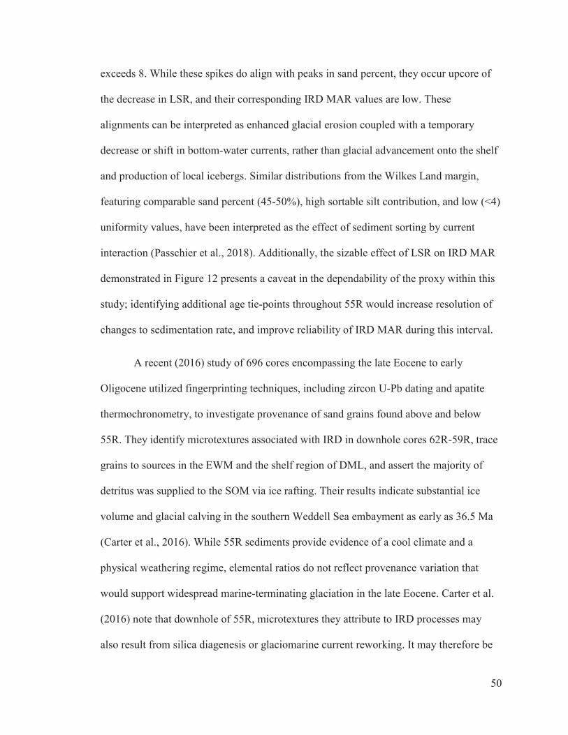
50
exceeds 8. While these spikes do align with peaks in sand percent, they occur upcore of
the decrease in LSR, and their corresponding IRD MAR values are low. These
alignments can be interpreted as enhanced glacial erosion coupled with a temporary
decrease or shift in bottom-water currents, rather than glacial advancement onto the shelf
and production of local icebergs. Similar distributions from the Wilkes Land margin,
featuring comparable sand percent (45-50%), high sortable silt contribution, and low (<4)
uniformity values, have been interpreted as the effect of sediment sorting by current
interaction (Passchier et al., 2018). Additionally, the sizable effect of LSR on IRD MAR
demonstrated in Figure 12 presents a caveat in the dependability of the proxy within this
study; identifying additional age tie-points throughout 55R would increase resolution of
changes to sedimentation rate, and improve reliability of IRD MAR during this interval.
A recent (2016) study of 696 cores encompassing the late Eocene to early
Oligocene utilized fingerprinting techniques, including zircon U-Pb dating and apatite
thermochronometry, to investigate provenance of sand grains found above and below
55R. They identify microtextures associated with IRD in downhole cores 62R-59R, trace
grains to sources in the EWM and the shelf region of DML, and assert the majority of
detritus was supplied to the SOM via ice rafting. Their results indicate substantial ice
volume and glacial calving in the southern Weddell Sea embayment as early as 36.5 Ma
(Carter et al., 2016). While 55R sediments provide evidence of a cool climate and a
physical weathering regime, elemental ratios do not reflect provenance variation that
would support widespread marine-terminating glaciation in the late Eocene. Carter et al.
(2016) note that downhole of 55R, microtextures they attribute to IRD processes may
also result from silica diagenesis or glaciomarine current reworking. It may therefore be
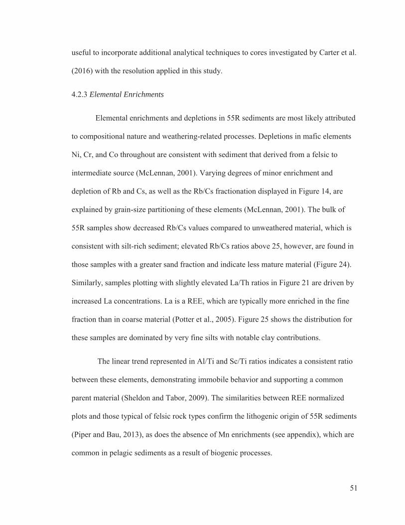
51
useful to incorporate additional analytical techniques to cores investigated by Carter et al.
(2016) with the resolution applied in this study.
4.2.3 Elemental Enrichments
Elemental enrichments and depletions in 55R sediments are most likely attributed
to compositional nature and weathering-related processes. Depletions in mafic elements
Ni, Cr, and Co throughout are consistent with sediment that derived from a felsic to
intermediate source (McLennan, 2001). Varying degrees of minor enrichment and
depletion of Rb and Cs, as well as the Rb/Cs fractionation displayed in Figure 14, are
explained by grain-size partitioning of these elements (McLennan, 2001). The bulk of
55R samples show decreased Rb/Cs values compared to unweathered material, which is
consistent with silt-rich sediment; elevated Rb/Cs ratios above 25, however, are found in
those samples with a greater sand fraction and indicate less mature material (Figure 24).
Similarly, samples plotting with slightly elevated La/Th ratios in Figure 21 are driven by
increased La concentrations. La is a REE, which are typically more enriched in the fine
fraction than in coarse material (Potter et al., 2005). Figure 25 shows the distribution for
these samples are dominated by very fine silts with notable clay contributions.
The linear trend represented in Al/Ti and Sc/Ti ratios indicates a consistent ratio
between these elements, demonstrating immobile behavior and supporting a common
parent material (Sheldon and Tabor, 2009). The similarities between REE normalized
plots and those typical of felsic rock types confirm the lithogenic origin of 55R sediments
(Piper and Bau, 2013), as does the absence of Mn enrichments (see appendix), which are
common in pelagic sediments as a result of biogenic processes.
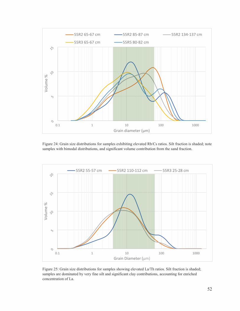
52
Figure 24: Grain size distributions for samples exhibiting elevated Rb/Cs ratios. Silt fraction is shaded; note samples with bimodal distributions, and significant volume contribution from the sand fraction.
Figure 25: Grain size distributions for samples showing elevated La/Th ratios. Silt fraction is shaded; samples are dominated by very fine silt and significant clay contributions, accounting for enriched concentration of La.
0.1 1 10 100 1000
Volu
me
%
Grain diameter (μm)
55R2 65-67 cm 55R2 85-87 cm 55R2 134-137 cm
55R3 65-67 cm 55R5 80-82 cm
0.1 1 10 100 1000
Volu
me
%
Grain Diameter (μm)
55R2 55-57 cm 55R2 110-112 cm 55R3 25-28 cm
53
Zr and Hf both show slight enrichments throughout 55R. These elements are
typically associated with heavy mineral assemblages like zircon and rutile, and are more
commonly enriched in the coarse fraction (silt, fine sands) than in the clay fraction
(McLennan, 2001; McLennan et al., 1993). Enrichments are therefore consistent with
55R samples which are dominated by silt. Zr enrichments may also be explained by
addition of zircon via sediment recycling (McLennan et al., 1993); Zr/Sc versus Th/Sc
ratios of 55R samples and discrimination fields from McLennan et al. (1993), however,
indicate Zr enrichment is more likely attributed to grain size partitioning than sediment
recycling (Figure 26). This serves to strengthen the validity of the biostratigraphic age
Figure 26: Th/Sc versus Zr/Sc plot demonstrating Zr enrichments in 55R samples are not likely attributed to zircon addition through sediment recycling (McLennan et al., 1993). Shaded region represents values of the UCC.
0.1 1 10 100 1000
Th/S
c
Zr/Sc
55R 1-5
54
model applied to Site 696 (Houben et al., 2013), as recycling of late Eocene dinocyst
assemblages found downhole is also unlikely. Furthermore, active margin samples are
less susceptible to recycling and these results are therefore consistent with Th/U versus
Th plots (McLennan et al., 1993).
5. CONCLUSIONS
The multi-method analysis of well-dated shelf sediments from the SOM spanning
the EOT presented here improves the understanding of glacial dynamics in the Weddell
Sea sector across this climate transition. From 34.3 to 33.52 Ma, the northern Antarctic
Peninsula and SOM were experiencing a cool, arid climate dominated by a physical
weathering regime. Sedimentation in this region was heavily influenced by wet-based
mountain glaciation, as evidenced by substantial contribution of glacial rock flour and
CIA values below 65 throughout the core. Peaks of significant sand contribution indicate
glaciers were orbitally influenced and cyclically advanced into valleys and perhaps even
terminated at the coast. While these results agree with evidence for alpine and potentially
tidewater glaciers in the Peninsula during the late Eocene (Anderson et al., 2011), the low
sedimentation rates following 34.1 Ma at Site 696 are not consistent with those associated
with full-scale glacial conditions in the Weddell Sea sector (Huang et al., 2014).
Recent investigations into Site 696 sediment provenance through the Late
Eocene-Early Oligocene identify East and West Antarctic sources and grain transport as
IRD (Carter et al., 2016), but geochemical and sedimentological analysis within 55R
suggests a local origin. Felsic/mafic ratios most resemble mudstones of the northern
Antarctic Peninsula, and Th/U vs. Th values plot analogously to those associated with
active margin muds. Sediment exhibits low uniformity throughout, suggesting that while
55
regional glacial advance provided the initial mechanism for erosion, transport and sorting
were controlled by other processes; possibilities include turbidity currents and sorting by
bottom current winnowing. Similar sorting and weathering processes are also attributed
to elemental enrichments and depletions, rather than changes in sediment provenance.
Core 55R sediments show evidence for significant glacial presence in the
northwest region of the Weddell Sea throughout the EOT, consistent with results of
similar studies in the Prydz Bay, Wilkes Land Margin, and Sabrina Coast regions
(Passchier et al., 2017; Light, 2017; Gulick et al., 2017). These results therefore support
large-scale regional cooling and glacial expansion prior to the ~34 Ma boundary.
Continuing high-resolution analyses of well-dated, shelf-proximal sediments allows
scientists to continue piecing together Antarctica’s glacial history. In doing so, we
improve both our understanding of ice dynamics during past times of great climate
change, and our abilities to assess the magnitude of ice response to modern warming.
56
6. REFERENCES
Anderson, J.B., 1999. Geologic History of Antarctica. Antarctic Marine Geology. Cambridge University Press.
Anderson, J.B. et al., 2011. “Progressive Cenozoic cooling and the demise of Antarctica’s last refugium”. PNAS. 108(28): 11356-11360.
Barker, P.F., Kennett, J.P., et al., 1988. Proceedings of the Ocean Drilling Program, Initial Reports, 113. Ocean Drilling Program, College Station, Texas.
Boggs, Jr, S., 2011. “Principles of Sedimentology and Stratigraphy”. 5th edition., Pearson.
Böning, P. et al., 2005. “Geochemical characteristics of Chilean upwelling sediments at ~36°S”. Marine Geology. 220(1-4):1-21.
Busetti, M. et al., 2000. “Geological Structure of the South Orkney Microcontinent”. Terra Antarctica. 8(2): 71-78.
Carter, A. et al., 2016. “Widespread Antarctic glaciation during the Late Eocene”. Earth and Planetary Science Letters. 458(2017):49-57.
Castillo, P. et al., 2014. “Petrography and geochemistry of the Carboniferous-Triassic Trinity Peninsula Group, West Antarctica: implications for provenance and tectonic setting”. Geological Magazine.152(4):575-588.
Cowan, E.A. et al., 2008. “Coarse-grained terrigenous sediment deposition on continental rise drifts: A record of Plio-Pleistocene glaciation on the Antarctic Peninsula”. Palaeogeography, Palaeoclimatology, Palaeoecology. 265(3-4): 275-291.
Coxall, H. et al., 2005. “Rapid stepwise onset of Antarctic glaciation and deeper calcite compensation in the Pacific Ocean”. Nature. 433: 53-57.
Coxall, H. and Wilson, P., 2011. “Early Oligocene glaciation and productivity in the eastern equatorial Pacific: Insights into global carbon cycling”. Paleoceanography and Paleoclimatology. 26(2).
DeConto, R.M. and Pollard, D., 2003. “Rapid Cenozoic glaciation of Antarctic induced by declining atmospheric CO2”. Nature. 421 (6920): 245-249.
Duprat, L.P.A.M., et al., 2016. “Enhanced Southern Ocean marine productivity due to fertilization by giant icebergs”. Nature Geoscience. 9: 219-221.
Eagles, G. and Livermore, R.A., 2002. “Opening history of Powell Basin, Antarctic Peninsula”. Marine Geology. 185: 195-205.
Feakins, S.J. et al., 2014. “Snapshot of cooling and drying before onset of Antarctic glaciation”. Earth and Planetary Science Letters. 404(2014): 154-166.
Fitzgerald, P. A. U. L., 2002. "Tectonics and landscape evolution of the Antarctic plate since the breakup of Gondwana with an emphasis on the West Antarctic Rift
57
System and the Transantarctic Mountains." Royal Society of New Zealand Bulletin. 35: 453-469.
Floyd, P.A. and Leveridge, B.E., 1987. “Tectonic environment of the Devonian Gramscatho basin, South Cornwall: framework mode and geochemical evidence from turbiditic sandstones”. Journal of the Geological Society, London. 144: 531-542.
Francis, J.E. et al., 2008. “100 Million Years of Antarctic Climate Evolution: Evidence from Fossil Plants”. Antarctica: A Keystone in a Changing World. Proceedings of the 10th International Symposium on Antarctic Earth Sciences. 19-26.
Francis, J.E. et al., 2009. “From Greenhouse to Icehouse – the Eocene/Oligocene in Antarctica”. In: Developments in Earth & Environmental Sciences. Chapter 8: 309-368. Elsevier B.V.
Galeotti, S. et al., 2016. “Antarctic Ice Sheet variability across the Eocene-Oligocene boundary climate transition”. Science. 354(6281):76-80.
Gromet, L.P. et al., 1984. “The ‘North American Shale Composite’: Its compilation, major and trace element characteristics”. Geochimica et Cosmochimica Acta. 48: 2469-2482.
Grützner, J., 2003. Data report: Multisensor core logging data, coarse-fraction grain-size analyses, and biogenic silica content of upper Miocene-lower Pliocene sediments, ODP Site 1165. In Cooper, A.K., O'Brien, P.E., and Richter, C. (Eds.), Proc. ODP, Sci. Results, 188.
Gulick, S.P.S. et al., 2017. “Initiation and long-term instability of the East Antarctic Ice Sheet”. Nature. 552: 225-229.
Hebbeln, D., 2000. “Flux of ice-rafted detritus from sea ice in the Fram Strait”. Deep-Sea Research. 47: 1773-1790.
Houben, A.J.P. et al., 2011. “Malvinia escutiana, a new biostratigraphically important Oligocene dinoflagellate cyst from the Southern Ocean”. Review of Palaeobotany and Palynology. 165: 175-182.
Houben, A.J.P. et al., 2012. “The Eocene-Oligocene transition: Changes in sea level, temperature or both?”. Palaeogeography, Palaeoclimatology, Palaeoecology. 335: 75-83.
Houben, A.J.P. et al., 2013. “Reorganization of Southern Ocean Plankton Ecosystem at the Onset of Antarctic Glaciation”. Science. 340: 341-344.
Huang, X. et al., 2014. “Variability in Cenozoic sedimentation and paleo-water depths of the Weddell Sea basin related to pre-glacial and glacial conditions of Antarctica”. Global and Planetary Change. 118: 25-41.
Ivany, L.C. et al., 2006. “Evidence for an earliest Oligocene ice sheet on the Antarctic Peninsula”. Geology. 34(5): 377-380.
58
Katz, M.E. et al., 2008. “Stepwise transition from the Eocene greenhouse to the Oligocene icehouse”. Nature Geoscience. 1:329-332.
King, E.C. and Barker, P.F., 1988. “The margins of the South Orkney Microcontinent”. Journal of the Geological Society. 145(2): 317-331.
Konert, M. and Vandenberghe, J., 1997. “Comparison of laser grain size analysis with pipette and sieve analysis: a solution for the underestimation of the clay fraction”. Sedimentology. 44(3): 523-535.
Krissek, L.A., 1998. “Data Report: Mass Accumulation Rates and Composition of Neogene Ice-Rafted Debris, Site 919, Irminger Basin”. Proceedings of the Ocean Drilling Program, Scientific Results. 163: 157-161.
Lear, C.H., et al., 2008. “Cooling and ice growth across the Eocene-Oligocene transition”. Geology. 36: 251-254.
Lee, H.M. et al., 2012. “The A-type Pirrit Hills Granite, West Antarctica: an example of magmatism associated with the Mesozoic break-up of the Gondwana supercontinent”. Geosciences Journal. 16(4): 421-433.
Light, J., 2017. “Geochemical and Particle Size Analysis of East Antarctic shelf sediments through the Eocene Oligocene Transition”. Montclair: Montclair State University.
Livermore, R. et al., 2005. “Paleogene opening of Drake Passage”. Earth and Planetary Science Letters. 236: 459-470.
Ma, L. et al., 2011. “Geochemical behaviors of different element groups during shale weathering at the Susquehanna/Shale Hills Critical Zone Observatory”. Applied Geochemistry. 26: 589-593.
McLennan, S.M et al., 1993. “Geochemical approaches to sedimentation, provenance, and tectonics”. Geological Society of America: Special Paper. 284: 21-40.
McLennan, S.M., 2001. “Relationships between the trace element composition of sedimentary rocks and upper continental crust”. Geochemistry Geophysics Geosystems. 2: paper number 2000GC000109.
Middelburg, J.J., 1988. “Chemical processes affecting the mobility of major, minor, and trace elements during weathering of granitic rocks”. Chemical Geology. 68: 253-273.
Miller, K.G. et al., 2009. “Climate threshold at the Eocene-Oligocene transition: Antarctic ice sheet influence on ocean circulation”. The Geological Society of America Special Paper. 452: 169-178.
Misra, K.C., 2012. “Introduction to Geochemistry: Principles and Applications, First Edition”. Blackwell Publishing Ltd.
“Moisture and Density”. Janus Data (Exp. 1-312). International Ocean Discovery Program.
59
Murray, R.W. et al., 2000. “Analysis of major and trace elements in rocks, sediments, and interstitial waters by inductively coupled plasma-atomic emission spectrometry (ICP-AES)”. ODP Technical Note, 29.
Naish, T., 2017. “What does the United Nations Paris Climate Agreement Mean for Antarctica?: Implications for New Zealand’s future research priorities”. Antarctic: The Publication of the New Zealand Antarctic Society. 35(4): 46-51.
Nakamura, N., 1974. “Determination of REE, Ba, Fe, Mg, Na and K in carbonaceous and ordinary chondrites”. Geochimica et Cosmochimica Acta. 38(5): 757-775.
Nesbitt, W. and G.M. Young, 1982. “Early Proterozoic Climates and Plate Motions Inferred from Major Element Chemistry of Lutites”. Nature. 299(9885): 715-717.
Pagani, M. et al., 2005. “Marked Decline in Atmospheric Carbon Dioxide Concentrations During the Paleogene”. Science. 309(5734): 600-603.
Pälike, H. et al., 2006. “The Heartbeat of the Oligocene Climate System”. Science. 314(5807): 1894-1898.
Passchier, S., 2011. “Linkages between East Antarctic Ice Sheet extent and Southern Ocean temperatures based on a Pliocene high-resolution record of ice-rafted debris off Prydz Bay, East Antarctica”. Paleoceanography and Paleoclimatology. 26(4): 1-13.
Passchier, S. et al., 2017. “An Antarctic stratigraphic record of stepwise ice growth through the Eocene-Oligocene transition”. Bulletin of the Geological Society of America. 129(3-4): 318-330.
Passchier, S. et al., 2018. “Sedimentary processes and facies on a high-latitude passive continental margin, Wilkes Land, East Antarctica”. Glaciated Margins: The Sedimentary and Geophysical Archive. The Geological Society of London. 475: 1-21.
Paulsson, O. and Austrheim, H., 2003. “A geochronological and geochemical study of rocks from Gjelsvikfjella, Dronning Maud Land, Antarctica – implications for Mesoproterozoic correlations and assembly of Gondwana”. Precambrian Research. 125: 113-138.
Pearce, J A., 1983. Role of the sub-continental lithosphere in magma genesis at active continental margins. In C.J Hawkesworth and M.J. Norry, Eds., Continental basalts and mantle xenoliths. Shiva, Orpington (London), and Birkhauser Boston, Cambridge, Massachusetts.
Pearson, P.N. et al., 2009. “Atmospheric carbon dioxide through the Eocene-Oligocene climate transition”. Nature. 461: 1110-1113.
Piper, D.Z. and Bau, M., 2013. “Normalized Rare Earth Elements in Water, Sediments, and Wine: Identifying Sources and Environmental Redox Conditions”. American Journal of Analytical Chemistry. 4: 69-83.
60
Potter, P.E., Maynard, J.B., & Depetris, P.J. Mud and mudstones: Introduction and overview. Springer Science & Business Media, 2005.
Robert, C. and Maillot, H., 1990. “Paleoenvironments in the Weddell Sea area and Antarctic climates, as deduced from clay mineral associations and geochemical data, ODP Leg 113”. In Proceedings of the Ocean Drilling Program, Scientific Results, Vol. 113. 51-70.
Rose, K.C. et al., 2013. “Early East Antarctic Ice Sheet growth recorded in the landscape of the Gamburtsev Subglacial Mountains”. Earth and Planetary Science Letters. 375: 1-12.
Sheldon, N.D. and Tabor, N.J., 2009. “Quantitative paleoenvironmental and paleoclimatic reconstruction using paleosols”. Earth-Science Reviews. 95: 1-52.
Sperazza, M. et al., 2004. “High-resolution particle size analysis of naturally occurring very fine-grained sediment through laser diffractometry”. Journal of Sedimentary Research. 74(5): 345-370.
Stocchi, P. et al., 2013. “Relative sea-level rise around East Antarctica during Oligocene glaciation”. Nature Geoscience. 6: 380-384.
Storti, F. and Balsamo, F., 2010. “Particle size distributions by laser diffraction: sensitivity of granular matter strength to analytical operation procedures”. Solid Earth. 1: 25-48.
Tamura, A. et al., 2015. “Measurement of whole-rock trace-element composition by flux-free fused glass and LA-ICP-MS: Evaluation of simple and rapid routine work”. Geochemical Journal. 49(3): 243-258.
Thiry, M., 2000. “Palaeoclimatic interpretations of clay minerals in marine deposits: an outlook from the continental origin”. Earth-Science Reviews. 49(1-4): 201-221.
Vandenberghe, N. et al., 2012. “The Paleogene Period”. The Geologic Time Scale 2012. By: Felix M. Gradstein. Amsterdam: Elsevier Science. 855-921.
Vennum, W.R. and Rowley, P.D., 1986. “Reconnaissance geochemistry of the Lassiter Coast Intrusive Suite, southern Antarctic Peninsula”. Geological Society of America Bulletin. 97: 1521-1533.
Vennum, W.R. and Storey, B.C., 1987. “Petrology, geochemistry, and tectonic setting of granitic rocks from the Ellsworth-Whitmore Mountains crustal block and Thiel Mountains, West Antarctica”. Geophysical Monograph Series: Structure, Tectonics, and Geophysics. Published by the American Geophysical Union. 40: 139-150.
Wang, C. et al., 2013. “The Eocene-Oligocene climate transition in the Tarim Basin, Northwest China: Evidence from clay mineralogy”. Applied Clay Science. 74:10-19.
Wedepohl, K.H., 1985. “The composition of the continental crust”. Geochimica et Cosmochimica Acta. 59(7): 1217-1232.
61
Wei, W. and Wise, S.W., 1990. “Middle Eocene to Pleistocene calcareous nanofossil recovered by Ocean Drilling Program Leg 113 in the Weddell Sea. Proc. ODP, Init. Rep., 113: 639-666.
Wentworth, C.K., 1922. “A scale of grade and class terms for clastic sediments”. United States Geological Survey. Hosted by: University of Chicago Press Journals. 377-392.
Will, T.M. et al., 2010. “Geochemical and isotopic constraints on the tectonic and crustal evolution of the Sheckleton Range, East Antarctica, and correlation with other Gondwana crustal segments”. Precambrian Research. 180: 85-112.
Williams, T. et al., 2010. “Evidence for iceberg armadas from East Antarctica in the Southern Ocean during the late Miocene and early Pliocene”. Earth and Planetary Science Letters. 290(3-4): 351-361.
Wilson, D.S. et al., 2012. “Antarctic topography at the Eocene-Oligocene boundary”. Palaeogeography, Palaeoclimatology, Palaeoecology. 335: 24-34.
Zachos, J., et al., 2001. “Trends, Rhythms, and Aberrations in Global Climate 65 Ma to Present”. Science. 292: 686-692.
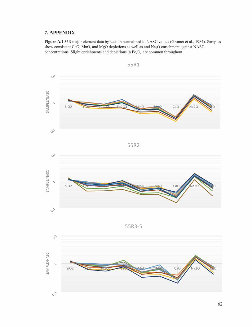
62
7. APPENDIX
Figure A.1 55R major element data by section normalized to NASC values (Gromet et al., 1984). Samples show consistent CaO, MnO, and MgO depletions as well as and Na2O enrichment against NASC concentrations. Slight enrichments and depletions in Fe2O3 are common throughout.
SiO2 TiO2 Al2O3 Fe2O3 MnO MgO CaO Na2O K2O
SAM
PLE/
NASC
55R1
SiO2 TiO2 Al2O3 Fe2O3 MnO MgO CaO Na2O K2O
SAM
PLE/
NASC
55R2
SiO2 TiO2 Al2O3 Fe2O3 MnO MgO CaO Na2O K2O
SAM
PLE/
NASC
55R3-5
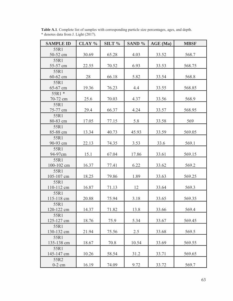
63
Table A.1. Complete list of samples with corresponding particle size percentages, ages, and depth. * denotes data from J. Light (2017).
SAMPLE ID CLAY % SILT % SAND % AGE (Ma) MBSF 55R1
50-52 cm 30.69 65.28 4.03 33.52 568.7 55R1
55-57 cm 22.55 70.52 6.93 33.53 568.75 55R1
60-62 cm 28 66.18 5.82 33.54 568.8 55R1
65-67 cm 19.36 76.23 4.4 33.55 568.85 55R1 *
70-72 cm 25.6 70.03 4.37 33.56 568.9 55R1
75-77 cm 29.4 66.37 4.24 33.57 568.95 55R1
80-83 cm 17.05 77.15 5.8 33.58 569 55R1
85-88 cm 13.34 40.73 45.93 33.59 569.05 55R1
90-93 cm 22.13 74.35 3.53 33.6 569.1 55R1
94-97cm 15.1 67.04 17.86 33.61 569.15 55R1
100-102 cm 16.37 77.41 6.22 33.62 569.2 55R1
105-107 cm 18.25 79.86 1.89 33.63 569.25 55R1
110-112 cm 16.87 71.13 12 33.64 569.3 55R1
115-118 cm 20.88 75.94 3.18 33.65 569.35 55R1
120-122 cm 14.37 71.82 13.8 33.66 569.4 55R1
125-127 cm 18.76 75.9 5.34 33.67 569.45 55R1
130-132 cm 21.94 75.56 2.5 33.68 569.5 55R1
135-138 cm 18.67 70.8 10.54 33.69 569.55 55R1
145-147 cm 10.26 58.54 31.2 33.71 569.65 55R2
0-2 cm 16.19 74.09 9.72 33.72 569.7
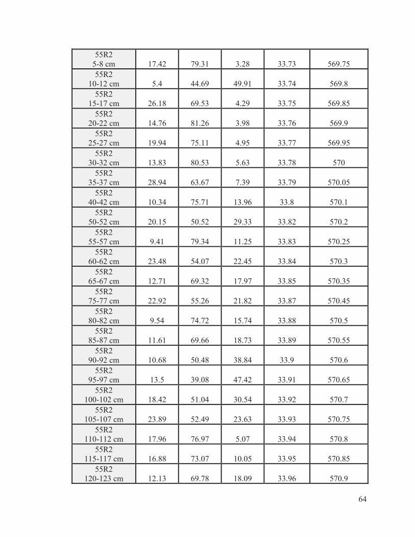
64
55R2 5-8 cm 17.42 79.31 3.28 33.73 569.75 55R2
10-12 cm 5.4 44.69 49.91 33.74 569.8 55R2
15-17 cm 26.18 69.53 4.29 33.75 569.85 55R2
20-22 cm 14.76 81.26 3.98 33.76 569.9 55R2
25-27 cm 19.94 75.11 4.95 33.77 569.95 55R2
30-32 cm 13.83 80.53 5.63 33.78 570 55R2
35-37 cm 28.94 63.67 7.39 33.79 570.05 55R2
40-42 cm 10.34 75.71 13.96 33.8 570.1 55R2
50-52 cm 20.15 50.52 29.33 33.82 570.2 55R2
55-57 cm 9.41 79.34 11.25 33.83 570.25 55R2
60-62 cm 23.48 54.07 22.45 33.84 570.3 55R2
65-67 cm 12.71 69.32 17.97 33.85 570.35 55R2
75-77 cm 22.92 55.26 21.82 33.87 570.45 55R2
80-82 cm 9.54 74.72 15.74 33.88 570.5 55R2
85-87 cm 11.61 69.66 18.73 33.89 570.55 55R2
90-92 cm 10.68 50.48 38.84 33.9 570.6 55R2
95-97 cm 13.5 39.08 47.42 33.91 570.65 55R2
100-102 cm 18.42 51.04 30.54 33.92 570.7 55R2
105-107 cm 23.89 52.49 23.63 33.93 570.75 55R2
110-112 cm 17.96 76.97 5.07 33.94 570.8 55R2
115-117 cm 16.88 73.07 10.05 33.95 570.85 55R2
120-123 cm 12.13 69.78 18.09 33.96 570.9

65
55R2 125-127 cm 21.20 72.29 6.51 33.97 570.95
55R2 130-133 cm 8.66 58.09 33.26 33.98 571
55R2 134-137 cm 14.21 74.94 10.85 33.99 571.05
55R2 140-143 cm 14.07 80.08 5.85 34 571.1
55R2 145-147 cm 16.91 79.96 3.13 34.01 571.15
55R3 5-7 cm 17.65 78.02 4.33 34.04 571.25 55R3
25-28 cm 20.88 73.9 5.22 34.08 571.45 55R3
35-37 cm 19.25 62.24 18.51 34.09 571.55 55R3
45-47 cm 17.40 46.28 36.33 34.1 571.65 55R3
55-57 cm 20.97 73.4 5.63 34.11 571.75 55R3
65-67 cm 24.29 70.6 5.11 34.12 571.85 55R3
90-92 cm 16.48 66.1 17.42 34.13 572.1 55R3
110-112 cm 25.94 68.9 5.16 34.14 572.3 55R3
135-137 cm 15.95 66.27 17.78 34.15 572.55 55R4
5-7 cm 20.80 63.08 16.11 34.16 572.75 55R4
25-27 cm 17.41 63.35 19.25 34.17 572.95 55R4
35-37 cm 13.88 54.1 32.02 34.175 573.05 55R4
45-47 cm 19.77 56.32 23.91 34.18 573.15 55R4
56-59 cm 15.03 45.98 38.99 34.185 573.25 55R4
65-67 cm 13.18 61.88 24.95 34.19 573.35 55R4
75-77 cm 21.14 62.03 16.83 34.195 573.45 55R4
90-92 cm 17.76 77.52 4.72 34.2 573.6
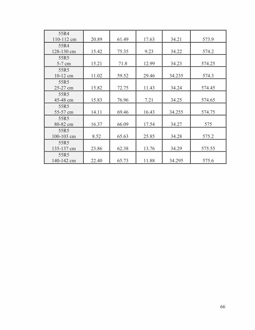
66
55R4 110-112 cm 20.89 61.49 17.63 34.21 573.9
55R4 128-130 cm 15.42 75.35 9.23 34.22 574.2
55R5 5-7 cm 15.21 71.8 12.99 34.23 574.25 55R5
10-12 cm 11.02 59.52 29.46 34.235 574.3 55R5
25-27 cm 15.82 72.75 11.43 34.24 574.45 55R5
45-48 cm 15.83 76.96 7.21 34.25 574.65 55R5
55-57 cm 14.11 69.46 16.43 34.255 574.75 55R5
80-82 cm 16.37 66.09 17.54 34.27 575 55R5
100-103 cm 8.52 65.63 25.85 34.28 575.2 55R5
135-137 cm 23.86 62.38 13.76 34.29 575.55 55R5
140-142 cm 22.40 65.73 11.88 34.295 575.6
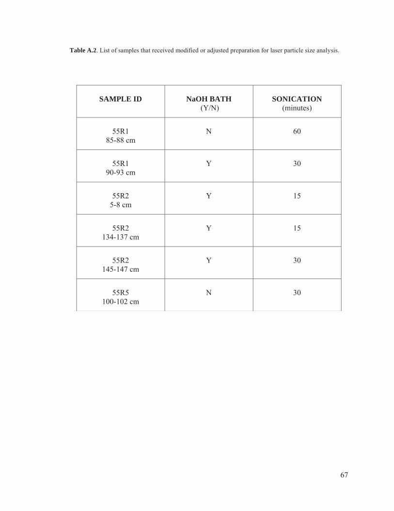
67
Table A.2. List of samples that received modified or adjusted preparation for laser particle size analysis.
SAMPLE ID
NaOH BATH
(Y/N)
SONICATION
(minutes)
55R1
85-88 cm
N
60
55R1
90-93 cm
Y
30
55R2
5-8 cm
Y
15
55R2
134-137 cm
Y
15
55R2
145-147 cm
Y
30
55R5
100-102 cm
N
30
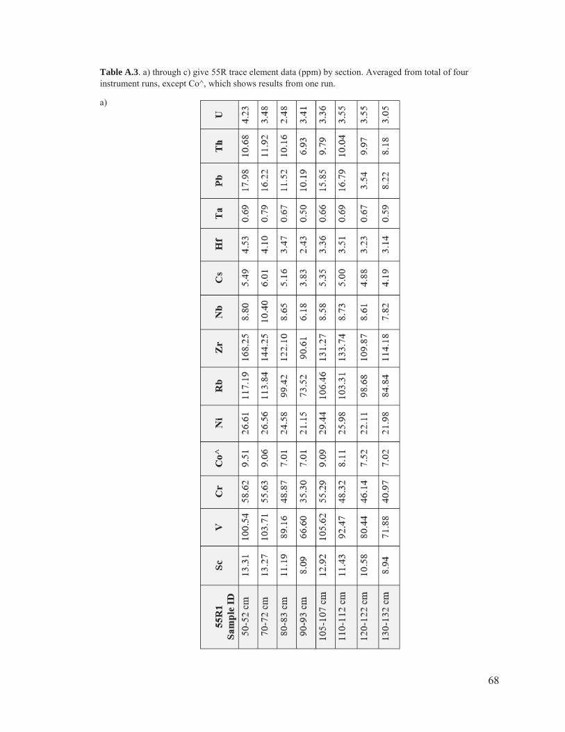
68
Table A.3. a) through c) give 55R trace element data (ppm) by section. Averaged from total of four instrument runs, except Co^, which shows results from one run.
a)
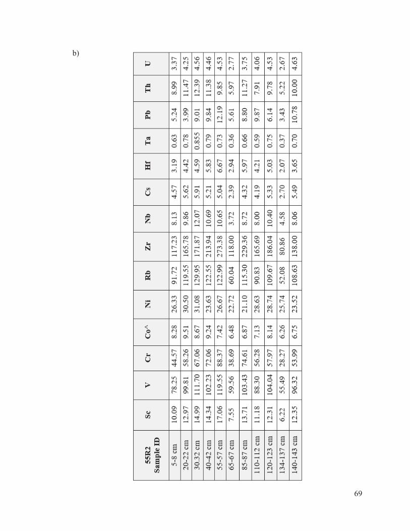
69
b)
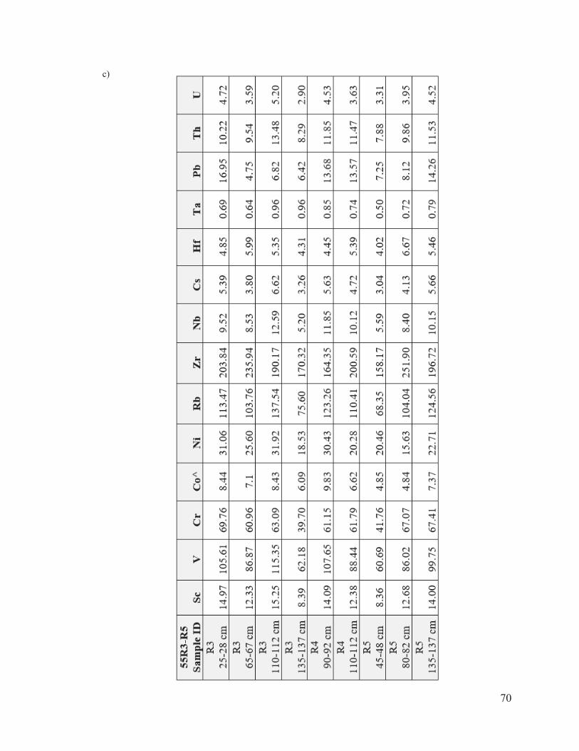
70
c)

71
Table A.4. a) through c) give 55R rare earth element concentrations (ppm) by section as averaged from four instrument runs.
a)
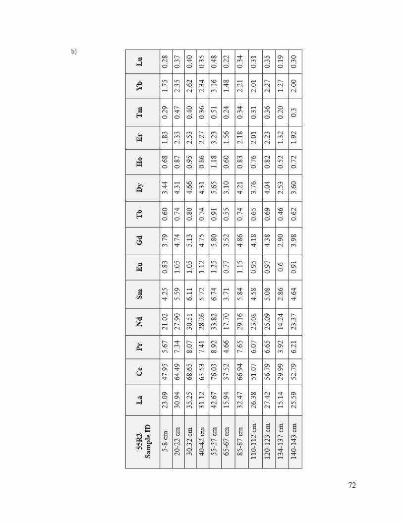
72
b)
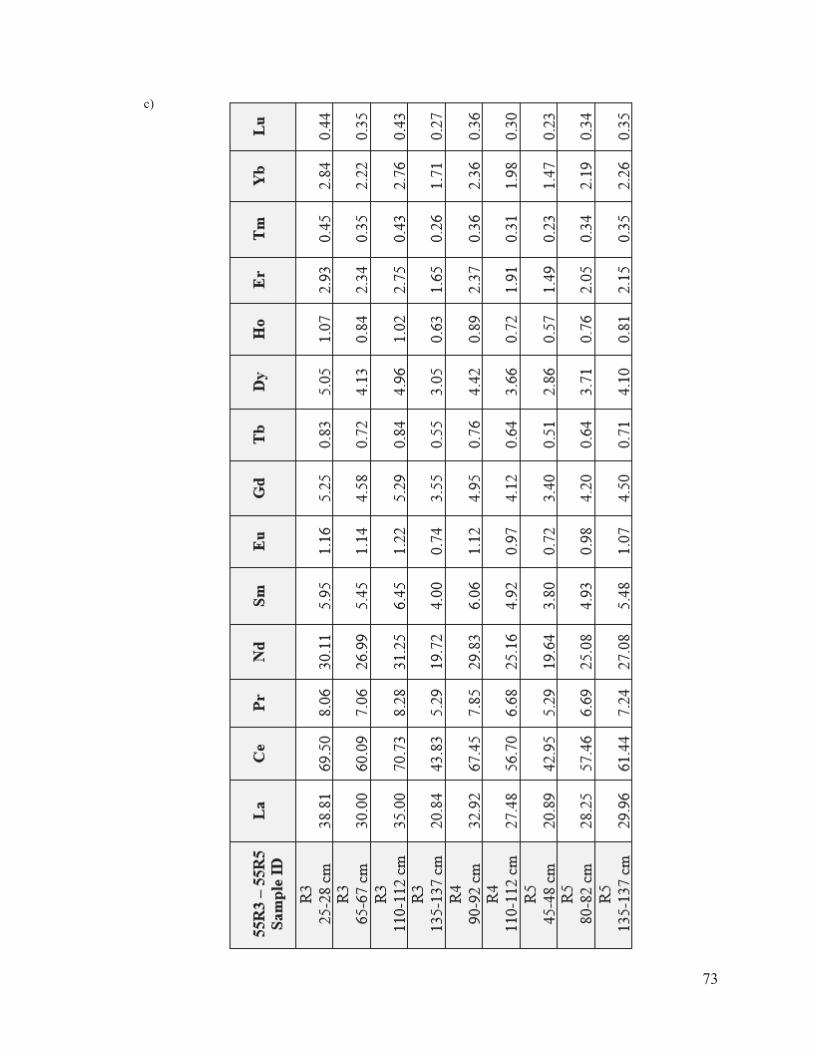
73
c)
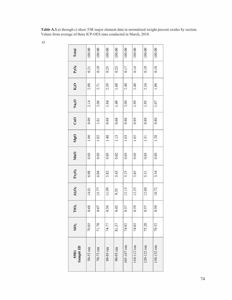
74
Table A.5.a) through c) show 55R major element data in normalized weight percent oxides by section. Values from average of three ICP-OES runs conducted in March, 2018.
a)
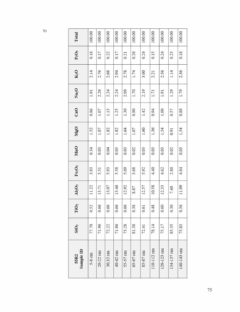
75
b)
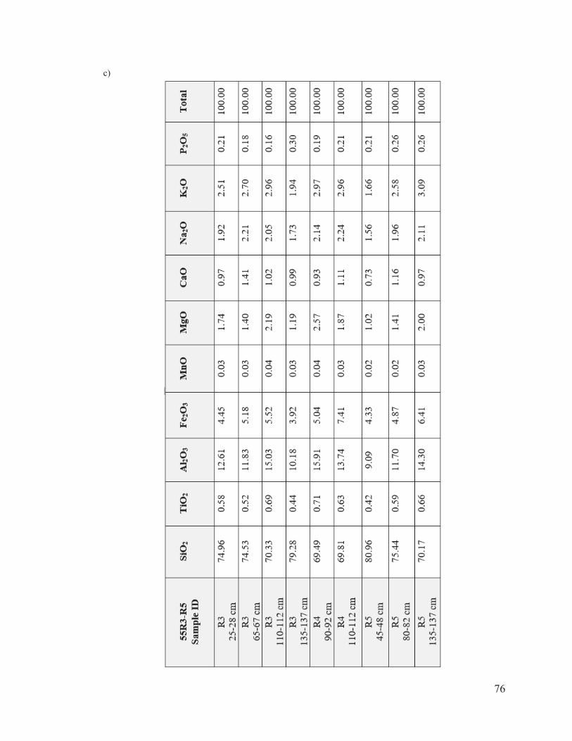
76
c)


