
Higgs Physics and Cosmology
By
Alex Roberts
A dissertation submitted in partial satisfaction of the
requirements of the degree of
Doctor of Philosophy
in
Physics
in the
Graduate Division
of the
University of California, Berkeley
Committee in charge:
Professor Yasunori Nomura, ChairProfessor Lawrence HallProfessor Chung-Pei Ma
Spring 2016

c© 2016 Alex Roberts

Abstract
Higgs Physics and Cosmology
by
Alex Roberts
Doctor of Philosophy in Physics
University of California, Berkeley
Professor Yasunori Nomura, Chair
Recently, a new framework for describing the multiverse has been proposed which is based onthe principles of quantum mechanics. The framework allows for well-defined predictions, bothregarding global properties of the universe and outcomes of particular experiments, accordingto a single probability formula. This provides complete unification of the eternally inflatingmultiverse and many worlds in quantum mechanics. We elucidate how cosmological parameterscan be calculated in this framework, and study the probability distribution for the value ofthe cosmological constant. We consider both positive and negative values, and find that theobserved value is consistent with the calculated distribution at an order of magnitude level. Inparticular, in contrast to the case of earlier measure proposals, our framework prefers a positivecosmological constant over a negative one. These results depend only moderately on how wemodel galaxy formation and life evolution therein.
We explore supersymmetric theories in which the Higgs mass is boosted by the non-decouplingD-terms of an extended U(1)X gauge symmetry, defined here to be a general linear combina-tion of hypercharge, baryon number, and lepton number. Crucially, the gauge coupling, gX , isbounded from below to accommodate the Higgs mass, while the quarks and leptons are requiredby gauge invariance to carry non-zero charge under U(1)X . This induces an irreducible rate,σBR, for pp → X → `` relevant to existing and future resonance searches, and gives rise tohigher dimension operators that are stringently constrained by precision electroweak measure-ments. Combined, these bounds define a maximally allowed region in the space of observables,(σBR, mX), outside of which is excluded by naturalness and experimental limits. If naturalsupersymmetry utilizes non-decoupling D-terms, then the associated X boson can only be ob-served within this window, providing a model independent ‘litmus test’ for this broad class ofscenarios at the LHC. Comparing limits, we find that current LHC results only exclude regionsin parameter space which were already disfavored by precision electroweak data..
Recent LHC data, together with the electroweak naturalness argument, suggest that the topsquarks may be significantly lighter than the other sfermions. We present supersymmetric modelsin which such a split spectrum is obtained through “geometries”: being “close to” electroweaksymmetry breaking implies being “away from” supersymmetry breaking, and vice versa. Inparticular, we present models in 5D warped spacetime, in which supersymmetry breaking andHiggs fields are located on the ultraviolet and infrared branes, respectively, and the top multipletsare localized to the infrared brane. The hierarchy of the Yukawa matrices can be obtained while
1

keeping near flavor degeneracy between the first two generation sfermions, avoiding stringentconstraints from flavor and CP violation. Through the AdS/CFT correspondence, the modelscan be interpreted as purely 4D theories in which the top and Higgs multiplets are compositesof some strongly interacting sector exhibiting nontrivial dynamics at a low energy. Becauseof the compositeness of the Higgs and top multiplets, Landau pole constraints for the Higgsand top couplings apply only up to the dynamical scale, allowing for a relatively heavy Higgsboson, including mh = 125 GeV as suggested by the recent LHC data. We analyze electroweaksymmetry breaking for a well-motivated subset of these models, and find that fine-tuning inelectroweak symmetry breaking is indeed ameliorated. We also discuss a flat space realization ofthe scenario in which supersymmetry is broken by boundary conditions, with the top multipletslocalized to a brane while other matter multiplets delocalized in the bulk.
2

Dedicated to my parents, Almut and Lutz.
Grateful also to you, Craig.
Love matters.
i

Acknowledgments
I would like to thank my advisor, Yasunori Nomura. I’m grateful for the opportunity to be able
to work with him. Our time working together at Berkeley and Santa Barbara has been fun. He
was good at teaching the material and involved Grant and I in discussing the direction of our
research approach. He agreed to pursue a promising idea when other professors would not have
been interested and it ended up being an important part of our publication (publication 1 in the
previous section).
I also thank Grant Larsen for being a great office-mate in Santa Barbara and for many useful
discussions. His odd sense of humour made him a great person to work with every day. I want
to thank Sean Weinberg for being a good roommate at UC Berkeley. We didn’t have a chance
to work together but I was interested in what you were pursuing at the time. I enjoyed frequent
discussions with Clifford Cheung both at UC Berkeley and the KITP in Santa Barbara. While
I didn’t stay for the entire 4 hour talk by your PhD adviser at the KITP, I learned a lot from
discussing ideas on gravity and supersymmetry with you. I was very impressed by how much
you can do in Mathematica and I am thankful for all the insights and discussions that eventually
turned into a paper (publication 3 in the previous section). I want to thank Asimina Arvanitaki,
Savas Dimopoulos, Joshua Ruderman and Satoshi Shirai for discussions and all the people in the
particle group at UC Berkeley. The lunch meetings were great and we had a good time reading
out paper abstracts and discussing ideas while we were having lunch. I also enjoyed the dinners
with speakers that we had often. I had the opportunity to try raw squid and other delicacies
and I only had to pay for the drinks.
I want to thank Prof. Christian Bauer for working with me on the GENEVA project, on the
adaptive sampling of the Monte Carlo generator. I’m grateful for the opportunity to work with
Simone Alioli and Jonathan Walsh on this project and to even be able to teach a new post-doc
on the details of what I had been doing. I want to thank Prof. Holger Muller for working with
me for a summer on his research.
ii

Contents
1 Introduction 1
1.1 The Cosmological Constant in the Quantum Multiverse . . . . . . . . . . . . . . 1
1.2 Higgs Mass from D-Terms: a Litmus Test . . . . . . . . . . . . . . . . . . . . . . 2
1.3 Supersymmetry with Light Stops . . . . . . . . . . . . . . . . . . . . . . . . . . 3
2 The Cosmological Constant in the Quantum Multiverse 6
2.1 Probabilities in the Quantum Mechanical Multiverse . . . . . . . . . . . . . . . 6
2.2 Predicting/Postdicting Cosmological Parameters . . . . . . . . . . . . . . . . . . 8
2.3 Approximating Observers . . . . . . . . . . . . . . . . . . . . . . . . . . . . . . 10
2.4 Distribution of the Cosmological Constant . . . . . . . . . . . . . . . . . . . . . 13
2.5 Conclusions . . . . . . . . . . . . . . . . . . . . . . . . . . . . . . . . . . . . . . 16
3 Higgs Mass from D-Terms: a Litmus Test 17
3.1 Setup . . . . . . . . . . . . . . . . . . . . . . . . . . . . . . . . . . . . . . . . . . 17
3.2 Results . . . . . . . . . . . . . . . . . . . . . . . . . . . . . . . . . . . . . . . . . 22
3.2.1 Experimental Constraints . . . . . . . . . . . . . . . . . . . . . . . . . . 22
3.2.2 Litmus Tests . . . . . . . . . . . . . . . . . . . . . . . . . . . . . . . . . 26
3.3 Conclusions . . . . . . . . . . . . . . . . . . . . . . . . . . . . . . . . . . . . . . 28
4 Supersymmetry with Light Stops 28
4.1 Formulation in Warped Space . . . . . . . . . . . . . . . . . . . . . . . . . . . . 28
4.1.1 The basic structure . . . . . . . . . . . . . . . . . . . . . . . . . . . . . . 28
4.1.2 Physics of flavor—fermions and sfermions . . . . . . . . . . . . . . . . . . 32
4.1.3 4D interpretation . . . . . . . . . . . . . . . . . . . . . . . . . . . . . . . 34
4.2 Electroweak Symmetry Breaking . . . . . . . . . . . . . . . . . . . . . . . . . . . 36
4.3 Overview . . . . . . . . . . . . . . . . . . . . . . . . . . . . . . . . . . . . . . . . 36
4.3.1 Higgs sector: κSUSY . . . . . . . . . . . . . . . . . . . . . . . . . . . . . 37
4.3.2 Sample spectra . . . . . . . . . . . . . . . . . . . . . . . . . . . . . . . . 41
4.4 Flat Space Realization . . . . . . . . . . . . . . . . . . . . . . . . . . . . . . . . 45
4.5 Conclusions . . . . . . . . . . . . . . . . . . . . . . . . . . . . . . . . . . . . . . 46
A Press-Schechter Formalism and Fitting Functions 53
B Anthropic Condition from Metallicity 55
C Analytical Formulae for the Higgs Boson Mass 57
iii

List of Tables
1. The probability of observing a positive and negative cosmological constant. . . 14
List of Figures
1. The normalized probability distribution of the vacuum energy. . . 15
2. Same as Fig. 2, but the horizontal axis now in logarithmic scale . . . 15
3. The normalized probability distribution P (ρΛ) with the metallicity condition . . . 16
4. The final normalized probability distribution P (ρΛ) with a metallicity condition. . . . 17
5. Litmus test: parameter space excluded by precision electroweak measurements (red), Higgs
mass limits (green), and LHC resonance searches (blue) at√s = 7 TeV . . . 18
6. Same as Fig. 6 except with√s = 14 TeV, and stop mass contours mt = 0.5 TeV, 2 TeV
. . . 19
7. Contours of gX,min which set the lower bound on gX required to raise the Higgs mass to
mh ' 125 GeV . . . 20
8. Contours of gX,max which set the upper bound on gX dictated by precision electroweak
constraints . . . 21
9. Contours of σBR/g2X in pb for mX = 3 TeV and
√s = 7 TeV . . . 22
10. Contours of σ/g2X in pb for
√s = 14 TeV . . . 23
11. Limits from precision electroweak measurements, and LHC resonance searches for p = q
and p 6= q free . . . 24
12. Same as Fig. 12, but for mt = 2 TeV . . . 25
13. Allowed regions for U(1)χ and U(1)3R . . . 26
14. A basic scheme yielding light stop spectra . . . 5
15. The 4D interpretation of the models. . . . 35
16. Two representative plots of the scalar mass spectrum in κSUSY . . . 39
17. Contours of the Higgs boson mass . . . 41
18. A typical mass spectrum for a compositeness scale of k′ = 10 TeV . . . 43
19. A typical mass spectrum for a compositeness scale of k′ = 1000 TeV . . . 44
20. The Higgs boson mass as a function of λ for fixed values of tan β and κ . . . 57
iv

1 Introduction
1.1 The Cosmological Constant in the Quantum Multiverse
An explanation of a small but nonzero cosmological constant is one of the major successes of the
picture that our universe is one of the many different universes in which low energy physical laws
take different forms [24]. Such a picture is also suggested theoretically by eternal inflation [25] and
the string landscape [26]. This elegant picture, however, has been suffering from the predictivity
crisis caused by an infinite number of events occurring in eternally inflating spacetime. To
make physical predictions, we need to deal with these infinities and define physically sensible
probabilities [27].
Recently, a well-defined framework to describe the eternally inflating multiverse has been
proposed based on the principles of quantum mechanics [28]. In this framework, the multiverse
is described as quantum branching processes viewed from a single “observer” (geodesic), and the
probabilities are given by a simple Born-like rule applied to the quantum state describing the
entire multiverse. Any physical questions—either regarding global properties of the universe or
outcomes of particular experiments—can be answered by using this single probability formula,
providing complete unification of the eternally inflating multiverse and many worlds in quantum
mechanics. Moreover, the state describing the multiverse is defined on the “observer’s” past
light cones bounded by (stretched) apparent horizons; namely, consistent description of the
entire multiverse is obtained in these limited spacetime regions. This leads to a dramatic change
of views on spacetime and gravity.
In this paper we present a calculation of the probability distribution of the cosmological
constant in this new framework of the quantum multiverse.1 We fix other physical parameters
and ask what values of the cosmological constant Λ we are likely to observe. In Section 2.1 we
begin by reviewing the proposal of Ref. [28], and we then explain how cosmological parameters
can be calculated in Section 2.2. While the framework itself is well-defined, any practical cal-
culation is necessarily approximate, since we need to model “experimenters” who actually make
observations. In our context, we need to consider galaxy formation and life evolution therein,
which we will do in Section 2.3. We present the result of our calculation in Section 2.4. We
find that, in contrast to the case with some earlier measures [34], the measure of Ref. [28] does
not lead to unwanted preference for a negative cosmological constant—in fact, a positive value
is preferred. We find that a simple anthropic condition based on metallicity of stars is sufficient
to make the calculated distribution consistent with the observed value at an order of magnitude
level. We conclude in Section 4.5.
Appendix A lists formulae for galaxy formation used in our analysis. Appendix B discusses
1For earlier studies of the cosmological constant in the context of geometric cutoff measures, see Refs. [29 – 33].
1

the anthropic condition coming from metallicity of stars.
1.2 Higgs Mass from D-Terms: a Litmus Test
Vital clues to the nature of electroweak symmetry breaking have emerged from the LHC. The
bulk of the standard model (SM) Higgs mass region has been excluded at 95% CL [1, 2], leaving a
narrow window 123 GeV < mh < 128 GeV in which there is a modest excess of events consistent
with mh ' 125 GeV. As is well-known, such a mass can be accommodated within the minimal
supersymmetric standard model (MSSM) but this requires large A-terms or very heavy scalars,
which tend to destabilize the electroweak hierarchy and undermine the original naturalness
motivation of supersymmetry (SUSY) [3, 4, 5]. Post LEP, however, a variety of strategies were
devised in order to lift the Higgs mass. In these models the Higgs quartic coupling is boosted:
either at tree level, via non-decoupling F-terms [6, 7, 8] and D-terms [9, 10], or radiatively, via
loops of additional matter [11, 12]. Already, a number of groups have redeployed these model
building tactics in light of the recent LHC Higgs results [5, 13, 14, 15].
The present work explores non-decoupling D-terms in gauge extensions of the MSSM. Our
aim is to identify the prospects for observing this scenario at the LHC in a maximally model
independent way. To begin, consider the MSSM augmented by an arbitrary flavor universal
U(1)X , which may be parameterized as a linear combination of hypercharge Y , Peccei-Quinn
number PQ, baryon number B, and lepton number L. The Higgs must carry X charge if the
corresponding D-terms are to contribute to the Higgs potential, so X must have a component
in Y or PQ. However, PQ forbids an explicit µ term, so gauging PQ requires a non-trivial
modification to the Higgs sector which is highly model dependent. To sidestep this complication
we ignore PQ and study the otherwise general space of U(1)X theories consistent with a µ term,
X = Y + pB − qL, (1)
where the normalization of X relative to Y has been absorbed into the sign and magnitude of
the gauge coupling, gX . We impose no further theoretical constraints, but will comment later
on anomalies, naturalness, and perturbative gauge coupling unification. As we will see, the
ultraviolet dynamics, e.g. the precise mechanism of gauge symmetry and SUSY breaking, will
be largely irrelevant to our analysis.
We constrain U(1)X with experimental data from resonance searches, precision electroweak
measurements, and Higgs results. Remarkably, non-trivial limits can be derived without exact
knowledge of seemingly essential parameters like gX , p, and q. This is possible because gX is
bounded from below by the mass of the Higgs while the couplings of the X boson to quarks,
leptons, and the Higgs are non-zero for all values of p and q. As a result, for a fixed value of the
X boson mass, mX , the theory predicts an irreducible rate, σBR, for the process pp→ X → ``
2

(relevant to direct searches) and an irreducible coupling of X to the Higgs and leptons (relevant
to precision electroweak data).
Combining limits, we derive a maximal allowed region in the space of observables, (σBR,mX),
outside of which is either unnatural or in conflict with experimental bounds, as shown in Figs. 6
and 7. If non-decoupling D-terms indeed play a role in boosting the Higgs mass, then the X
boson can only be observed within this allowed region—a ‘litmus test’ for this general class of
theories. Furthermore, we find that for natural SUSY, i.e. mt . 500 GeV, resonance searches
from the LHC [16] are not yet competitive with existing precision electroweak constraints.
In Sec. 3.1 we define our basic setup. Applying the constraints of gauge symmetry and
SUSY, we derive a general expression for the Higgs potential arising from non-decoupling D-
terms. Afterwards, in Sec. 3.2 we compute the Higgs mass and the couplings of the MSSM
fields to the X boson. We then impose experimental limits and suggest a simple litmus test for
non-decoupling D-terms. We conclude in Sec. 3.3.
1.3 Supersymmetry with Light Stops
One of the strongest motivations for weak scale supersymmetry is the possibility of making elec-
troweak symmetry breaking “natural,” i.e. a generic parameter region of the theory reproduces
observed electroweak phenomena. With the Higgs potential V (h) = m2h†h + λ(h†h)2/4, the
minimization of the potential leads to v ≡ 〈h〉 =√−2m2/λ and
m2h
2= −m2, (2)
where mh is the physical Higgs boson mass. In the Standard Model (SM) a generic size of |m2|is expected to be at a scale where the theory breaks down, while in supersymmetric models
m2 = |µ|2 + m2h, (3)
where µ and m2h are the supersymmetric and supersymmetry-breaking masses for the Higgs field.
Therefore, as long as these parameters are both of order the weak scale, the theory can naturally
accommodate electroweak symmetry breaking.
Improved experimental constraints over the past decades, however, have cast doubt on this
simple picture. In softly broken supersymmetric theories, supersymmetry-breaking masses are
affected by each other through renormalization group evolution; in particular, mh receives a
contribution
δm2h ' −
3m2t
4π2v2m2t ln
Mmess
mt
, (4)
where mt and mt are the top quark and squark masses, and Mmess the scale at which su-
persymmetry breaking masses are generated. (Here, we have ignored possible scalar trilinear
3

interactions and set the left- and right-handed squark masses equal, for simplicity.) Requiring
no more fine-tuning than ∆, Eqs. (2) and (3) lead to
mt<∼ 420 GeV
(mh
125 GeV
)(20%
∆−1
)1/2(3
ln Mmess
mt
)1/2
. (5)
On the other hand, recent observations at the LHC indicate:
• Generic lower bounds on the first two generation squark masses are about 1 TeV [50].
• There are hints of the SM-like Higgs boson with mh ' 125 GeV [51].
Therefore, if the hints for the Higgs boson mass are true, then it strongly suggests that the
squark masses have a nontrivial flavor structure, i.e. top squarks (stops) are light.2
The above observation has significant implications on an underlying model of supersymmetry
breaking. This is especially because many existing models, including minimal supergravity, gauge
mediation, and anomaly mediation, invoke flavor universality to avoid stringent constraints from
the absence of large flavor violating processes. On the other hand, it has been realized that
naturalness itself allows sfermions other than the stops (and the left-handed sbottom) to be
significantly heavier than the value suggested by Eq. (5) [53, 54, 55, 56, 57, 58]. In this paper,
we study a simple, general framework in which such superparticle spectra with light stops are
obtained naturally.
One strategy to yield such light stop spectra is to arrange the theory in such a way that being
“away” from electroweak symmetry breaking necessarily means being “close” to supersymmetry
breaking, and vice versa. This makes the lighter generations (particles feeling smaller effects from
electroweak symmetry breaking) obtain larger supersymmetry breaking masses, e.g. of order a
few TeV, while keeping stops light. Strong constraints from flavor violation still require the first
two generation sfermions to be flavor universal, but this can be achieved if these generations are
both strongly localized to the supersymmetry breaking “site,” and if mediation of supersymmetry
breaking there is flavor universal. The setup described here is depicted schematically in Fig. 1.
A simple way to realize the above setup is through geometry. Suppose there is an extra
dimension compactified on an interval, of which the Higgs and supersymmetry breaking fields h
and X are localized at the opposite ends. The SM gauge, quark, and lepton multiplets propagate
in the bulk. Now, if two generations are localized towards the “X brane” and (at least the quark
2One way of avoiding this conclusion is to invoke a significant mixing of the Higgs field with another scalar field;see [52]. In general, mixing of the SM-like Higgs field with another field can weaken the naive constraint, Eq. (5),obtained in the decoupling regime (at the cost of moderate cancellation in a scalar mass-squared eigenvalue).Another possibility is to have a relatively compressed superparticle spectrum, in particular a small mass splittingbetween the squarks and the lightest neutralino, in which case the lower bound on the (light generation) squarkmasses becomes weaker.
4

Figure 1: A basic scheme yielding light stop spectra. A theory has one “dimension,” of whichelectroweak and supersymmetry breakings are “located” at the opposite ends. This dimensionmay be geometric or an effective one generated through dynamics. The first two generationfields are localized towards the supersymmetry breaking “site,” obtaining flavor universal super-symmetry breaking masses and only small effects from electroweak symmetry breaking (smallYukawa couplings). On the other hand, top-quark multiplets are localized more towards theelectroweak breaking “site,” obtaining a large Yukawa coupling but only small supersymmetrybreaking effects.
doublet and up-type quark of) the other generation is localized towards the “h brane,” then it
explains the (anti-)correlation between the spectrum of SM matter and its superpartners—the
hierarchy of the Yukawa couplings are generated through the wavefunction overlap of SM matter
with the h brane, while only the first two generation sfermions obtain significant supersymmetry
breaking masses through interactions with the X brane.
Another manifestation of this is through dynamics—the “dimension” separating two break-
ings in Fig. 1 may be generated effectively as a result of strong (quasi-)conformal dynamics.
Suppose there are elementary as well as composite sectors. In this case, particles in each sec-
tor interact with significant strength, but interactions involving both elementary and composite
particles are suppressed by higher dimensions of composite fields. This can therefore be used to
realize our setup, for example, by considering X and h to be elementary and composite fields,
respectively. The SM matter fields are mixture of elementary and composite states—two gen-
erations being mostly elementary while the other mostly composite. In this way, the required
pattern for the sfermion masses, as well as the hierarchical structure of the Yukawa couplings,
are obtained. In fact, this picture can be related with the geometric picture described above.
Since the strong, composite sector exhibits (approximate) conformality at high energies, the
dynamics is well described by a warped extra dimension, using the AdS/CFT correspondence.
(For applications of this idea in other contexts, see e.g. [59, 60, 61].)
In this paper, we present a class of models formulated in warped space, which can be in-
terpreted either as a geometric or dynamical realization described above. In the next section,
5

we present the basic structure of the models and interpret them as composite Higgs-top models
in the desert. We pay particular attention to how strong constraints from flavor violation are
avoided while generating the Yukawa hierarchy. In Section 4.2, we analyze electroweak symme-
try breaking and present sample superparticle spectra; we also give some useful formulae for the
Higgs boson mass in the appendix. In section 4.4, we mention a realization of our scheme in a
flat space extra dimension. We conclude in Section 4.5.
The configuration of supersymmetry breaking and matter/Higgs fields in our models is the
same as that in “emergent supersymmetry” models considered before [62, 63, 64], where the
masses of elementary superpartners m are taken (much) above the scale of strong dynamics k′.
In this picture, the quadratic divergence of the Higgs mass-squared parameter is regulated by
a combination of composite Higgsinos/stops as well as higher resonances of the strong sector
(Kaluza-Klein towers). Instead, our picture here is that the theory below the compositeness
scale is the full supersymmetric standard model, m < k′, so that the quadratic divergence of the
Higgs mass-squared is regulated by superpartner loops as in usual supersymmetric models—the
strong sector simply plays a role of generating a light stop spectrum at some energy k′. This
alleviates the problem of a potentially large D-term operator [63], intrinsic to the framework of
Ref. [62, 63, 64].
Three interesting papers have recently considered light stops in supersymmetry [65, 66, 67],
which are related to our study here. Ref. [65] discusses supersymmetric models in which the
Higgs, top, and electroweak gauge fields are (partial) composites of a strong sector that sits at
the bottom edge of the conformal window. This can be viewed as an explicit 4D realization of
our warped 5D setup. (This “analogy” has also been drawn in that paper.) Ref. [66] considers
the scheme of flavor mediation, where supersymmetry breaking is mediated through a gauged
subgroup of SM flavor symmetries, leading to degenerate light-generation sfermions with light
stops. Ref. [67] discusses light stops in the context of heterotic string theory.
2 The Cosmological Constant in the Quantum Multi-
verse
2.1 Probabilities in the Quantum Mechanical Multiverse
Here we review aspects of the framework of Ref. [28] which are relevant to our calculation. In
this framework, the entire multiverse is described as a single quantum state as viewed from
a single “observer” (geodesic). It allows us to make well-defined predictions in the multiverse
(both cosmological and terrestrial), based on the principles of quantum mechanics.
Let us begin by considering a scattering process in usual (non-gravitational) quantum field
theory. Suppose we collide an electron and a positron, with well-defined momenta and spins:
6

|e+e−〉 at t = −∞. According to the laws of quantum mechanics, the evolution of the state
is deterministic. In a relativistic regime, however, this evolution does not preserve the particle
number or species, so we find
Ψ(t = −∞) =∣∣e+e−
⟩→ Ψ(t = +∞) = ce
∣∣e+e−⟩
+ cµ∣∣µ+µ−
⟩+ · · · , (6)
when we expand the state in terms of the free theory states (which is appropriate for t → ±∞when interactions are weak). The Hilbert space of the theory is (isomorphic to) the Fock space
H =∞⊕n=0
H⊗n1P , (7)
where H1P is the single-particle Hilbert space. Various “final states,” |e+e−〉 , |µ+µ−〉 , · · · , in
Eq. (6) arise simply because the time evolution operator causes “hopping” between different
components of the Fock space in Eq. (7).
The situation in the multiverse is quite analogous. Suppose the universe was in an eternally
inflating (quasi-de Sitter) phase Σ at some early time t = t0. In general, the evolution of this
state is not along the axes determined by operators local in spacetime. Therefore, at late times,
the state is a superposition of different “states”
Ψ(t = t0) = |Σ〉 → Ψ(t) =∑i
ci(t) |(cosmic) configuration i〉 , (8)
when expanded in terms of the states corresponding to definite semi-classical configurations.
The Hilbert space of the theory is (isomorphic to)
H =⊕M
HM, HM = HM,bulk ⊗HM,horizon, (9)
where HM is the Hilbert space for a fixed semi-classical spacetime M, and consists of the bulk
and horizon parts HM,bulk and HM,horizon. (The quantum states are defined on the “observer’s”
past light cones bounded by apparent horizons.) The final state of Eq. (8) becomes a super-
position of different semi-classical configurations because the evolution operator for Ψ(t) allows
“hopping” between different HM in Eq. (9).
As discussed in detail in Ref. [28], any physical question can be phrased as: “Given what we
know about our past light cone, A, what is the probability of that light cone to have properties
B as well?” This probability is given by
P (B|A) =
∫dt 〈Ψ(t)| OA∩B |Ψ(t)〉∫dt 〈Ψ(t)| OA |Ψ(t)〉
, (10)
assuming that the multiverse is in a pure state |Ψ(t)〉. (The mixed state case can be treated
similarly.) Here, OA is the projection operator
OA =∑i
|αA,i〉 〈αA,i| , (11)
7

where |αA,i〉 represents a set of orthonormal states in the Hilbert space of Eq. (9), i.e. possible
past light cones, that satisfy condition A (and similarly for OA∩B). Despite the fact that the t
integrals in Eq. (10) run from t = t0 to ∞, the resulting P (B|A) is well-defined, since |Ψ(t)〉 is
continually “diluted” into supersymmetric Minkowski states [28].
The formula in Eq. (10) (or its mixed state version) can be used to answer questions both
regarding global properties of the universe and outcomes of particular experiments. This, there-
fore, provides complete unification of the two concepts: the eternally inflating multiverse and
many worlds in quantum mechanics [28].3 To predict/postdict physical parameters x, we need
to choose A to select the situation for “premeasurement” without conditioning on x. We can
then use various different values (ranges) of x for B, to obtain the probability distribution P (x).
In the next section, we discuss this procedure in more detail, in the context of calculating the
probability distribution of the vacuum energy, x = ρΛ ≡ Λ/8πGN .
2.2 Predicting/Postdicting Cosmological Parameters
In order to use Eq. (10) to predict/postdict physical parameters, we need to know the rele-
vant properties of both the state |Ψ(t)〉 (or its bulk part ρbulk ≡ Trhorizon |Ψ(t)〉 〈Ψ(t)|) and the
operators OA and OA∩B. Here we discuss them in turn.
In general, the state |Ψ(t)〉 depends on the dynamics of the multiverse, including the scalar
potential in the landscape, as well as the initial condition, e.g. at t = t0. Given limited current
theoretical technology, this introduces uncertainties in predicting physical parameters. However,
there are certain cases in which these uncertainties are under control. Consider x = ρΛ. We
are interested only in a range a few orders of magnitude around ρΛ,obs ' (0.0024 eV)4 [36],
which is tiny compared with the theoretically expected range −M4Pl<∼ ρΛ
<∼ M4Pl. Therefore,
unless the multiverse dynamics or initial condition has a special correlation with the value of the
vacuum energy in the standard model (SM) vacua, we expect that the probabilities of having
these vacua in |Ψ(t)〉 is statistically uniform in x within the range of interest. (This corresponds
to the standard assumption of statistical uniformity of the prior distribution of ρΛ [24].) The
distribution of x = ρΛ is then determined purely by the dynamics inside the SM universes,
i.e., the probability of developing experimenters who actually make observations of the vacuum
energies.
Let us now turn to the operators OA and OA∩B. In order to predict the value of the vacuum
energy which a given experimenter will observe, we need to choose OA to select a particular
3The claim that the multiverse and many worlds are the same has also been made recently in Ref. [35], but thephysical picture there is very different. Those authors argue that quantum mechanics has operational meaningonly under the existence of causal horizons because making probabilistic predictions requires decoherence withdegrees of freedom outside the horizons. Our picture does not require such an extra agent to define probabilities(or quantum mechanics). The evolution of our Ψ(t) is deterministic and unitary.
8

“premeasurement” situation for that experimenter, i.e.
P (ρΛ) dρΛ = P (B|A),
A : a particular “premeasurement” situationB : ρΛ < vacuum energy < ρΛ + dρΛ,
(12)
where P (B|A) is defined in Eq. (10). Here, we have assumed that the number of SM vacua
is sufficiently large for ρΛ to be treated as continuous in the range of interest. In general, the
specification of the premeasurement situation can be arbitrarily precise; for example, we can
consider a particular person taking a particular posture in a particular room, with the tip of the
light cone used to define |Ψ(t)〉 located at a particular point in space. In practice, however, we are
interested in the vacuum energy “a generic observer” will measure. We therefore need to relax
the condition we impose as A; in other words, we need to “coarse grain” the premeasurement
situation. In fact, some coarse graining is always necessary when we apply the formalism to
postdiction (see discussions in Ref. [28]).
What condition A should we impose then? To address this issue, let us take the semi-classical
picture of the framework, discussed in Section 2 of Ref. [28]. In this picture, the probability is
given by
P (B|A) = limn→∞
NA∩BNA
, (13)
where NA is the number of past light cones that satisfy A and are encountered by one of the
n geodesics emanating from randomly distributed points on the initial hypersurface at t = t0.
(This is equivalent to Eq. (10) in the regime where the semi-classical picture is valid.) Since
we vary only ρΛ, all the SM universes look essentially identical at early times when the vacuum
energy is negligible. The assumed lack of statistical correlation between ρΛ and the multiverse
dynamics then implies that we can consider a fixed number of geodesics emanating from a fixed
physical volume at an early time (e.g. at reheating) in these universes, and see what fraction of
these geodesics find the “premeasurement” situation A in each of these universes.
Given that we are focusing on the SM universes in which only the values of ρΛ are different,
it is reasonable to expect that all the experimenters look essentially identical for different ρΛ, at
least statistically—in particular, we assume that they have similar sizes, masses, and lifetimes.
With this “coarse graining,” the condition A can be taken, e.g., as: the geodesic intersects with
the body of an experimenter at some time during their life. In practice, this makes the probability
proportional to the fraction of a fixed comoving volume at an early time that later intersects
with the body of an observer. Note that the details of the condition A here do not matter for
the final results—for example, we can replace the “body” by “head” or “nose” without changing
the results because its effect drops out from the normalized probability. Thus, in this situation
(and any situation in which condition A can be formulated entirely in terms of things directly
encountered by the geodesic), the semi-classical approximation to the scheme of Ref. [28] can be
9

calculated as the fat geodesic measure outlined in Ref. [37].4 We emphasize that the consistent
quantum mechanical solution to the measure problem in Ref. [28] forces this choice on us.
We can now present the formula for P (ρΛ) in a more manageable form. Since the prob-
ability for one of the geodesics to intersect an experimenter is proportional to the number of
experimenters and the density of geodesics, we have
P (ρΛ) ∝∑
a∈habitable galaxies
Nobs,a ρgeod,a, (14)
where Nobs,a and ρgeod,a are, respectively, the total number of observers/experimenters and the
density of geodesics in a “habitable” galaxy a. Here, we have approximated that ρgeod,a is
constant throughout the galaxy a. Note that since we count intersections of experimenters with
geodesics, rather than just the number of observers (as in much previous work, e.g. [29]), our
results differ from such previous results by our factor of ρgeod,a. Our remaining task, then, is
to come up with a scheme that can “model” Nobs,a and ρgeod,a reasonably well so that the final
result is not far from the truth.
2.3 Approximating Observers
In this section, we convert Eq. (14) into an analytic expression that allows us to compute P (ρΛ)
numerically. We focus on presenting the basic logic behind our arguments. Detailed forms of
the functions appearing below, e.g. F (M, t) and H(t′;M, t), as well as useful fitting functions,
are given in Appendix A.
Let us begin with Nobs,a. We assume that, at a given time t, the number of observers arising
in a given galaxy a is proportional to the total number of baryons in a
dNobs,a
dt(t) ∝∼ NB,a(t), (15)
as long as stars are luminous. This assumption is reasonable if the rate of forming observers
is sufficiently small, which appears to be the case in our universe. To estimate the number of
baryons existing in galaxies, we use the standard Press-Schechter formalism [38], which provides
the fraction of matter collapsed into halos of mass larger than M by time t, F (M, t). Since the
amount of baryons collapsed is proportional to that of matter, we can use this function F to
estimate the number of observers and find5
P (ρΛ)?∝∼ −
∫dt
∫dM
dF (M, t)
dMρgeod(M, t). (16)
4To our knowledge, no detailed study of the probability distribution of the cosmological constant accordingto the fat geodesic measure has been published prior to this work.
5Note that the sign of dF/dM is negative because of the definition of F .
10

The expression of Eq. (16) does not take into account the fact that forming intelligent ob-
servers takes time, or that observers appear only when stars are luminous (which we postulate,
motivated by the assumption that we are typical observers). To include these effects, we use the
extended Press-Schechter formalism [39], which gives the probability H(t′;M, t) that a halo of
mass M at time t virialized before t′. The probability density P (ρΛ) can then be written as
P (ρΛ)?∝∼ −
∫dt
∫dM
dF (M, t)
dMH(t− tevol;M, t)−H(t− tburn;M, t) ρgeod(M, t), (17)
where tevol and tburn are the time needed for intelligent observers to evolve and the characteristic
lifetime of stars which limits the existence of life, respectively.
The density of geodesics ρgeod(M, t) is proportional to that of a dark matter halo of mass M
at time t, which is given by its average virial density:
ρgeod(M, t) ≈(dF (M, t∗)
dM
)−1 ∫ t∗
0
dt′ ρvir(t′)d2F (M, t′)
dMdt′, (18)
where t∗ = mint, tstop(M) with tstop(M) the time after which the number of halos of mass M
starts decreasing, i.e. when merging into larger structures dominates over formation of new halos:
d2F/dMdt|t=tstop(M) = 0. (For the explicit expression of ρvir, see Appendix A.) In the interest of
speeding up numerical calculation, we approximate this by the virial density at the time when
the rate of matter collapsing into a halo of mass M , i.e. −d2F/dMdt, becomes maximum:
ρgeod(M, t) ≈ ρvir(τ(M)) , (19)
where τ(M) is given byd3F (M, t)
dMdt2
∣∣∣∣t=τ(M)
= 0. (20)
This approximation is indeed reasonable at the level of precision we are interested in: it works
at the level of 20% for t >∼ 1.7τ(M) where the contribution to P (ρΛ) almost entirely comes from.
Finally, there will be several additional anthropic conditions for a halo to be able to host
intelligent observers. For example, the mass of a halo may have to be larger than some critical
value Mmin to efficiently form stars [40], and smaller than Mmax for the galaxy to be cooled
efficiently [41, 42]. Considering these factors, we finally obtain from Eqs. (17) and (19)
P (ρΛ) = − 1
N
∫ tf
tevol
dt
∫ Mmax
Mmin
dMdF (M, t)
dMH(t− tevol;M, t)−H(t− tburn;M, t) ρvir(τ(M))n(M, t),
(21)
where N is the normalization factor. Here,
tf =
∞ for ρΛ ≥ 0
tcrunch ≡√
π6GN |ρΛ|
for ρΛ < 0,(22)
11

and we have put anthropic conditions besides Mmin,max in the form of a function n. Note that F ,
H, and ρvir (and possibly n) all depend on the value of the vacuum energy ρΛ; see Appendix A.
In summary, (dF/dM) (H|t−tevol−H|t−tburn
)n dMdt counts the (expected) number of ob-
servers in halos with mass between M and M + dM at time between t and t + dt, and ρvir(τ)
is proportional to the density of geodesics in such a halo and time, and so Eq. (21) gives the
probability by counting their intersections (as in Eq. (14)), with n implementing some anthropic
conditions. One well-motivated origin for n is metallicity of stars, which affects the rate of planet
formation (see e.g. Refs. [43, 44]). Here we simply model this effect by multiplying some power
m of integrated star formation up to time t − tevol, which we assume to be proportional to the
integrated galaxy formation rate for M > Mmin:
n(M, t) ∝∼(F (Mmin,mint− tevol, tstop)− F (M,mint− tevol, tstop)
)m, (23)
where tstop is determined by dF (Mmin, t′)−F (M, t′)/dt′|t′=tstop
= 0. (For the derivation of this
expression, see Appendix B.) Motivated by the observation that the formation rate of certain
(though not Earth-like) planets is proportional to the second power of host star metallicity [44],
we consider the case m = 2, as well as m = 1.6
Another possible anthropic condition comes from the fact that if a halo is too dense, it
may not host a habitable solar system because of the effects of close encounters [46]. Following
Ref. [41], we assume this anthropic condition to take the form
n?σ†v† <∼1
tcr
, (24)
where n?, σ†, v†, and tcr are the density of stars, critical “kill” cross section, relative velocity of
encounters, and some timescale relevant for the condition. Since n? ∝ ρvir, v† ∼ vvir ∝M1/3ρ1/6vir ,
and σ† and tcr are (expected to be) independent of M and ρvir, this is translated into
n(M, t) = Θ
(ρmax − ρvir(τ(M))
( M
Mmin
)2/7), (25)
where Θ(x) is the step function (= 1 for x ≥ 0 and = 0 for x < 0), and we have normalized M
by Mmin.
The value of ρmax is highly uncertain. One way to estimate it is to follow Ref. [41] and take
n? ∼ (1 pc)−3( ρvir
ρvir,MW
), σ† ∼ πr2
AU, v† ∼ vvir ∼
√Tvir,MW
mp
( M
MMW
)1/3( ρvir
ρvir,MW
)1/6
, (26)
6There is observational data for metallicity of galaxies in our universe [45], which our crude model here does notreproduce quantitatively. However, when we straightforwardly extrapolate the empirical data to other universes,the same regions of the integrand in Eq. (21) are suppressed/enhanced so that the effect on our calculation isqualitatively the same. It must be noted, though, that the strength of the effect may change; e.g. P (ρΛ) for ourmodel with m = 1 is qualitatively similar to the distribution obtained using the observation-motivated methodwith m = 3.
12

where mp is the proton mass, rAU ' 1.5 × 10⁸ km is the Sun-Earth distance, and ρvir,MW ∼2 × 10⁻²⁶ g/cm3, Tvir,MW ∼ 5 × 10⁵ K, and MMW ∼ 1 × 10¹²M are the virial density, virial
temperature, and mass of the Milky Way galaxy, respectively. Using tcr ∼ tevol = 5 Gyr, Eq. (24)
leads to
ρmax ∼ 9× 10³ ρvir,MW
(MMW
Mmin
)2/7
∼ 3× 10⁻²² g/cm3. (27)
This corresponds to the constraint from direct encounters, i.e. the orbit of a planet being dis-
rupted by the passage of a nearby star. There can also be a constraint from indirect encounters:
a passing star perturbs an Oort cloud in the outer part of the solar system, triggering a lethal
comet impact [41]. For a fixed M , this constraint can be about four orders of magnitude stronger
than Eq. (27)
ρmax ∼ 3× 10⁻²⁶ g/cm3; (28)
namely, our Milky Way galaxy may lie at the edge of allowed parameter space.
In our analysis below, we consider either or both of the above conditions Eqs. (23) and (25). In
the real world, there are (almost certainly) more conditions needed for intelligent life to develop.
However, incorporating these conditions would likely improve the prediction/postdiction for ρΛ.
In this sense, our analysis may be viewed as a “conservative” assessment for the success of the
framework, although it is still subject to uncertainties coming from the modeling of observers.
2.4 Distribution of the Cosmological Constant
Our modeling of observers has several parameters which need to be determined phenomenolog-
ically: Eq. (21) contains Mmin, Mmax, tevol, and tburn, while Eq. (25) contains ρmax. We take the
“minimum” galaxy mass appearing in Eq. (21) to be
Mmin = 2× 10¹¹M, (29)
below which the efficiency of star formation drops abruptly [40]. For tevol, and tburn, we take
them approximately to be the age of the Earth and lifetime of the Sun, respectively:
tevol = 5 Gyr, tburn = 10 Gyr. (30)
In our analysis below, we use Eqs. (29) and (30); we do not impose the constraint from galaxy
cooling, i.e. we set Mmax = ∞. While the values of these parameters are highly uncertain, our
results are not very sensitive to these values. The dependence of our results on them will be
discussed at the end of this section. In Fig. 2, we present the normalized probability distribution
for the vacuum energy P (ρΛ) as a function of ρΛ/ρΛ,obs, under several assumptions about the
function n:
(i) “minimal” anthropic condition: n(M, t) = 1
13

P (ρΛ > 0) P (ρΛ < 0)No condition 97% 3%
Metallicity, m = 1 87% 13%Metallicity, m = 2 75% 25%
ρmax = 6× 10⁻²⁶ g/cm3 92% 8%ρmax = 4.5× 10⁻²⁶ g/cm3 83% 17%ρmax = 3× 10⁻²⁶ g/cm3 63% 37%
Table 1: The probability of observing a positive and negative cosmological constant, P (ρΛ > 0)and P (ρΛ < 0), for six assumptions on the anthropic condition. In all cases, a positive value ispreferred over a negative one, consistent with observation.
(ii) metallicity condition: Eq. (23) with m = 1 and 2
(iii) maximum virial density condition: Eq. (25) with ρmax = 3 × 10⁻²⁶, 4.5 × 10⁻²⁶, 6 ×10⁻²⁶ g/cm3, which are 1, 1.5, 2 times the value in Eq. (28).
(The result with ρmax given by Eq. (27) is virtually identical to the case with the minimal
anthropic condition.) The left panel presents the effects of metallicity, showing (i) and (ii),
while the right panel those of ρmax, with (i) and (iii).
Interestingly, in all cases, our predictions prefer a positive cosmological constant over a
negative one, as opposed to the situation in earlier measure proposals where strong preferences
to negative values have been found [34]. In Table 1, we provide the probabilities of having
ρΛ > 0 (and < 0) in all six anthropic scenarios. The absence of an unwanted preference towards
negative ρΛ is satisfactory, especially given that the measure of Ref. [28] was not devised to cure
this problem. It comes from the fact that the present measure does not have a large volume
effect associated with the global geometry of anti-de Sitter space, which was responsible for a
strong preference for negative ρΛ in earlier, geometric cutoff measures [34]. In contrast with these
measures, the quantum measure of Ref. [28] does not count the number of events; rather, it gives
quantum mechanical weights for “situations,” i.e. quantum mechanical states as described from
the viewpoint of a single observer (geodesic). The preference towards a positive value comes
from the fact that for ρΛ > 0 some observers still form after vacuum energy domination, while
for ρΛ < 0 it is not possible due to the big crunch.
Figure 2 shows that P (ρΛ) is always peaked near ρΛ = 0, with the distribution becoming
wider as the anthropic condition gets weaker. In Fig. 3, we plot the same distributions in
logarithmic scale for ρΛ/ρΛ,obs, limiting ourselves to ρΛ > 0. To show the probability density
per tenfold, the vertical axis is chosen as ρΛP (ρΛ)/ρΛ,obs. From these figures, we find that our
anthropic assumptions lead to results that are consistent with the observed value within one or
two orders of magnitude. In particular, metallicity alone is enough to bring the agreement to
14

-10 0 10 20 30 40ΡLΡL,obs
0.02
0.04
0.06
0.08
0.10
0.12
PHΡLL
-10 0 10 20 30 40ΡLΡL,obs
0.05
0.10
0.15
0.20
PHΡLL
Figure 2: The normalized probability distribution of the vacuum energy P (ρΛ) as a function ofρΛ/ρΛ,obs. The left panel shows P (ρΛ) with the metallicity condition, Eq. (23), with m = 0 (i.e.no condition; dashed, blue), m = 1 (dot-dashed, red), and m = 2 (solid, black). The right panelshows P (ρΛ) with the upper bound ρmax, Eq. (25), with ρmax = ∞ (i.e. no constraint; dashed,blue), 6×10⁻²⁶ g/cm3 (dotted, purple), 4.5×10⁻²⁶ g/cm3 (dot-dashed, red), and 3×10⁻²⁶ g/cm3
(solid, black).
0.1 1 10 100 1000ΡLΡL,obs0.0
0.1
0.2
0.3
0.4
0.5PHΡLLΡLΡL,obs
0.1 1 10 100 1000ΡLΡL,obs0.0
0.2
0.4
0.6
0.8PHΡLLΡLΡL,obs
Figure 3: Same as Fig. 2, but the horizontal axis now in logarithmic scale. To show the proba-bility density per tenfold, the vertical axis is chosen to be ρΛP (ρΛ)/ρΛ,obs. The distributions arenormalized in the region ρΛ > 0.
an order of magnitude level. This is because mergers, which lead to an increase in metallicity,
are suppressed for larger values of ρΛ due to earlier vacuum energy domination. This result is
comfortable, especially given that the constraint from encounters is effective only if ρmax is close
to the Milky Way value, as in Eq. (28). Given our crude treatment of observers, we consider
these results quite successful.
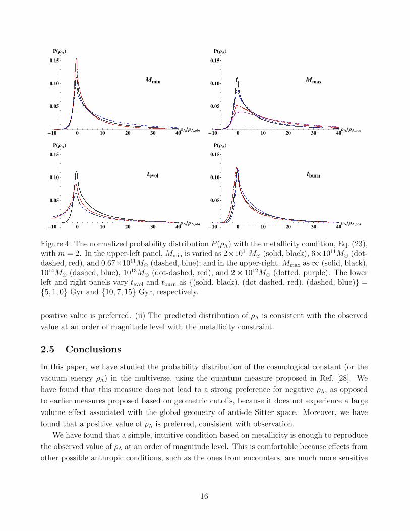
Finally, we discuss the sensitivity of our results to variations of Mmin, Mmax, tevol, and tburn,
which can be thought of as “systematic effects” of our analysis. In Fig. 4, we show the distri-
butions of P (ρΛ) with the m = 2 metallicity constraint, varying the values of Mmin, Mmax, tevol,
and tburn, respectively. We find that, while the detailed shape of P (ρΛ) does change, our main
conclusions are robust: (i) There is no strong preference to a negative vacuum energy; in fact, a
15
Mmin
-10 0 10 20 30 40ΡLΡL,obs
0.05
0.10
0.15
PHΡLL
Mmax
-10 0 10 20 30 40ΡLΡL,obs
0.05
0.10
0.15
PHΡLL
tevol
-10 0 10 20 30 40ΡLΡL,obs
0.05
0.10
0.15
PHΡLL
tburn
-10 0 10 20 30 40ΡLΡL,obs
0.05
0.10
0.15
PHΡLL
Figure 4: The normalized probability distribution P (ρΛ) with the metallicity condition, Eq. (23),with m = 2. In the upper-left panel, Mmin is varied as 2×10¹¹M (solid, black), 6×10¹¹M (dot-dashed, red), and 0.67×10¹¹M (dashed, blue); and in the upper-right, Mmax as∞ (solid, black),1014M (dashed, blue), 1013M (dot-dashed, red), and 2× 10¹²M (dotted, purple). The lowerleft and right panels vary tevol and tburn as (solid, black), (dot-dashed, red), (dashed, blue) =5, 1, 0 Gyr and 10, 7, 15 Gyr, respectively.
positive value is preferred. (ii) The predicted distribution of ρΛ is consistent with the observed
value at an order of magnitude level with the metallicity constraint.
2.5 Conclusions
In this paper, we have studied the probability distribution of the cosmological constant (or the
vacuum energy ρΛ) in the multiverse, using the quantum measure proposed in Ref. [28]. We
have found that this measure does not lead to a strong preference for negative ρΛ, as opposed
to earlier measures proposed based on geometric cutoffs, because it does not experience a large
volume effect associated with the global geometry of anti-de Sitter space. Moreover, we have
found that a positive value of ρΛ is preferred, consistent with observation.
We have found that a simple, intuitive condition based on metallicity is enough to reproduce
the observed value of ρΛ at an order of magnitude level. This is comfortable because effects from
other possible anthropic conditions, such as the ones from encounters, are much more sensitive
16

-10 0 10 20 30 40 50 60ΡLΡL,obs
0.02
0.04
0.06
0.08
0.10
0.12PHΡLL
Figure 5: The normalized probability distribution P (ρΛ) with a metallicity condition: Eq. (23)with m = 2. The light and dark shaded regions indicate those between 1 and 2σ, and outside2σ, respectively. The observed value ρΛ/ρΛ,obs = 1 (denoted by a vertical line) is consistent withthe distribution at the 1σ level.
to the details of the conditions. In Fig. 5, we present the normalized distribution P (ρΛ) with
the m = 2 metallicity constraint, where the 1 and 2σ regions are indicated. We find that the
observed value is consistent with the calculated distribution at the 1σ level.
It would be interesting to refine our analysis including more detailed anthropic effects, such as
those of star formation. Another possible extension of the analysis is to vary other cosmological
parameters, such as the primordial density contrast Q and spatial curvature Ωk (at a specified
time), in addition to ρΛ. We plan to study these issues in the future.
3 Higgs Mass from D-Terms: a Litmus Test
3.1 Setup
We are interested in all U(1)X extensions of the MSSM consistent with a gauge invariant µ
term. Mirroring [17, 20], we go to a convenient basis in which the charge parameters, gX ,
p, and q, absorb all of the effects of kinetic and mass mixing between the U(1)X and U(1)Y
gauge bosons above the electroweak scale. Thus, mixing only occurs after electroweak symmetry
breaking, and the resulting effects are proportional to the Higgs vacuum expectation value
(VEV). Of course, kinetic mixing is continually induced by running, so this choice of basis is
renormalization scale dependent. However, this subtlety is largely irrelevant to our analysis,
17

PEW
LHCHiggsMass
0.5TeV
1TeV
2TeV
10-6 10-5 10-4 10-3 10-2
1.6
1.8
2.0
2.2
2.4
2.6
2.8
3.0
ΣBR HpbL
mX
HTeV
L
s = 7 TeV
Figure 6: Litmus test: parameter space excluded by precision electroweak measurements (red), Higgs masslimits (green), and LHC resonance searches (blue) at
√s = 7 TeV. For σBR too large, gX > gX,max yielding
tension with precision electroweak and LHC constraints; for σBR too small, gX < gX,min yielding tension withmh ' 125 GeV subject to the stop mass, shown here for mt = 0.5 TeV, 1 TeV, 2 TeV. See the text in Sec. 3.2for details.
which involves experimental limits in a relatively narrow window of energies around the weak
scale. The advantage of this low energy parameterization is that it is very general and covers
popular gauge extensions like U(1)B, U(1)L, U(1)B−L, U(1)χ, and U(1)3R. Furthermore, it is
defined by a handful of parameters: mX , gX , p, and q.
Next, let us consider the issue of anomalies. If p = q, then according to Eq. (1) X is a
linear combination of the Y and B − L, which is anomaly free if one includes a flavor triplet of
right-handed neutrinos. If p 6= q then the associated B+L anomalies can be similarly cancelled
by new particles. In general, these ‘anomalons’ can be quite heavy, in which case they can be
ignored for our analysis.
We now examine the non-decoupling D-terms of U(1)X and their contribution to the Higgs
potential. As we will see, these contributions are highly constrained by gauge symmetry and
SUSY. To begin, consider a massive vector superfield composed of component fields
C, χ,X, λ,D, (31)
where X, λ, and D are the gauge field, gaugino, and auxiliary field, and C and χ are the
18

2
2
0.5 TeV
2 TeV
HiggsMass
PEW
10-6 10-5 10-4 10-3 10-2
2
3
4
5
ΣBR HpbL
mX
HTeV
L
s = 14 TeV
Figure 7: Same as Fig. 6 except with√s = 14 TeV, and stop mass contours mt = 0.5 TeV, 2 TeV.
‘longitudinal’ modes eaten during the super-Higgs mechanism. Under SUSY transformations,
C → C + i(ξχ− ξχ) (32)
D → D + ∂µ(−ξσµλ+ λσµξ). (33)
Eq. (33) implies that mC −D is a SUSY invariant on the equations of motion, iσµ∂µλ = mχ,
where m = mC = mλ = mX is the mass of the vector superfield.
On the other hand, the auxiliary field D can be re-expressed in terms of dynamically propa-
gating fields by substituting the equations of motion. Since mC −D is a SUSY invariant, this
implies that
D = mC +DIR +DUV +O(C2), (34)
where DIR and DUV label contributions from the (light) MSSM fields and the (heavy) U(1)X
breaking fields, respectively, with all C dependence shown explicitly. The structure of Eq. (34)
ensures that both the right and left hand sides transform the same under SUSY transformations.
In the normalization of Eq. (1), Hu,d has charge ±1/2 under U(1)X , which implies
DIR =gX2
(|Hu|2 − |Hd|2 + . . .). (35)
The effective potential for C and the MSSM scalars is obtained by setting all other fields to their
19

0.4
0.5
0.60.7
g
g'
0.5 1.0 1.5 2.0 2.5
10
20
30
40
50
mt HTeVL
tan
Β
gX,min
Figure 8: Contours of gX,min which set the lower bound on gX required to raise the Higgs mass to mh ' 125GeV. Values equal to the SM gauge couplings are highlighted.
VEVs, yielding
V =1
2D2 +
1
2m2C2 + tC. (36)
The first term is the usual SUSY D-term contribution, while the second and third terms arise
from soft SUSY breaking effects such as non-zero F-terms. Here we have dropped terms O(C3)
and higher because they are unimportant for the Higgs quartic. Note that the spurions m and
t depend implicitly on the VEVs of U(1)X breaking sector fields.
In the SUSY limit, m = t = 0 and integrating out C eliminates all DIR dependence in the
potential—no Higgs quartic is induced, as expected. If, on the other hand, t 6= 0, then C and
DUV will typically acquire messenger scale VEVs, yielding a huge tree-level contribution to mHu
and mHd through a term linear in DIR. To avoid a destabilization of the electroweak scale,
one usually assumes some ultraviolet symmetry, e.g. messenger parity, which ensures t = 0 and
vanishing VEVs for C and DUV. We assume this to be the case here, in which case there is no
D-term SUSY breaking.
On the other hand, SUSY breaking typically enters through m 6= 0, whose effects can be
characterized by a simple SUSY spurion analysis. Let us model m by an ultraviolet superfield
spurion for F-term breaking, θ2F . This spurion can effect the scalar sector in two ways: through
the indirect shifts of scalar component VEVs, or through the direct couplings of θ2F to super-
fields. In the former, the masses of C and X may vary, but they do so together, and the states
20

0.1
0.2
0.3
0.4
0.6
0.8
0.5
0.3
-2 -1 0 1 20.5
1.0
1.5
2.0
2.5
3.0
q
mX
HTeV
L
gX,max
Figure 9: Contours of gX,max which set the upper bound on gX dictated by precision electroweak constraints.These limits depend primarily on the couplings of X to leptons, which are set by the q parameter.
remain degenerate. In the latter, only certain couplings are permitted between θ2F and the vec-
tor superfield components. Simple θ and θ counting shows that X and D cannot couple directly
to θ2F , while C can. Hence, C is split in mass from the remainder of the gauge multiplet by
F-term SUSY breaking.
Putting this all together, we rewrite Eq. (36) as
V =1
2(mXC +DIR)2 +
1
2(m2
C −m2X)C2, (37)
where the coefficient of the second term is fixed so that mC is the physical mass of C. Note that
the prefactor for C in the first term is mX—this can be verified by explicit computation, and is
a direct consequence of the fact that X and D cannot couple directly to θ2F . Integrating out C
yields our final answer for the effective D-term contribution to the Higgs potential
V =1
2εD2
IR (38)
ε = 1−m2X/m
2C , (39)
which is a generalization of the specific examples in [9, 10]. In the SUSY limit, mC = mX
and the D-term contribution vanishes as expected. A positive contribution to the Higgs mass
requires positive ε, which in turn requires that mC > mX . Importantly, 0 ≤ ε < 1 independent
of the ultraviolet completion, which will be crucial later on when we derive model independent
bounds.
21

10-4.5
10-4
10-4
10-3.5
10-3.5
10-3.5
10-3
-2 -1 0 1 2-2
-1
0
1
2
q
p
ΣBR gX2
Figure 10: Contours of σBR/g2X in pb for mX = 3 TeV and
√s = 7 TeV. Irrespective of the U(1)X charge
parameters p and q, the rate is always non-zero.
3.2 Results
3.2.1 Experimental Constraints
In this section we analyze the experimental constraints on general U(1)X extensions of the
MSSM. The relevant bounds come from the mass of the Higgs boson, precision electroweak
measurements, and direct limits from the LHC.
• Higgs Boson Mass. Recent results from the LHC indicate hints of a SM-like Higgs boson
at around mh ' 125 GeV. Taken at face value, this imposes a stringent constraint on theories
of U(1)X D-terms. In particular, combining Eq. (35) with Eq. (39) yields the mass of the Higgs
boson
m2h = m2
Z cos2 2β
(1 +
εg2X
g′2 + g2
)+ δm2
h, (40)
where 0 ≤ ε < 1 independent of the ultraviolet completion. Here δm2h denotes the usual radiative
contributions to the Higgs mass in the MSSM,
δm2h =
3m4t
4π2v2
(log
m2t
m2t
+X2t
m2t
(1− X2
t
12m2t
)), (41)
where mt = (mt1mt2)1/2 and Xt = At − µ cot β. In our actual analysis we employ the analytic
expressions from [21] for the Higgs mass, which include two-loop leading log corrections.
22

10-3
10-2
10-1
1
101
-2 -1 0 1 2
2
3
4
5
6
p
mX
HTeV
L
Σ gX2
Figure 11: Contours of σ/g2X in pb for
√s = 14 TeV.
To simplify the parameter space, we take At = 0 and µ = 200 GeV. Our results will be
indicative of theories which have small A-terms, such as gauge mediated SUSY breaking. For a
given value of tan β and mt, the Higgs mass correction δm2h is then fixed. Using Eq. (40) and
0 ≤ ε < 1, we find that gX is bounded from below in order to accommodate mh ' 125 GeV:
gX > gX,min, (42)
where gX,min is a function of (mt, tan β) shown in Fig. 8. For comparison, this figure includes
contours of the SM electroweak gauge couplings, g′ and g. At high tan β, U(1)X is most effective
at lifting the Higgs mass, so the stop masses can be the smallest. Note that in certain ultraviolet
completions, ε can be quite small, in which case gX,min and thus gX will be much larger than the
SM gauge couplings.
Lastly, let us comment briefly on the issue of fine tuning. In Sec. 3.1 we showed that non-
decoupling D-terms require the scalar C to be split from the X boson at tree level. As a
consequence, the low energy Higgs quartic coupling behaves like a hard breaking of SUSY and
loops involving the components of the vector supermultiplet generate a quadratic divergence
which is cut off by mX . Since the Higgs fields are charged under U(1)X , these radiative cor-
rections contribute to the Higgs soft masses at one loop and can destabilize the electroweak
hierarchy. In particular,
δm2Hu,d
=g2X
64π2m2X log
(m6Xm
2C
m8λ
), (43)
23

PEW
LHC
-2 -1 0 1 2
1.5
2.0
2.5
3.0
q
mX
HTeV
L
mt = 0.5 TeV
Figure 12: Limits from precision electroweak measurements (red solid), and LHC resonance searches for p = q(blue dashed) and p 6= q free (blue shaded), with mt = 0.5 TeV, corresponding to gX > gX,min = 0.54. Directsearches only exclude regions already disfavored by precision electroweak constraints.
which applies to R-symmetric limit [18, 19]. As required, when the components of the supermul-
tiplet become degenerate, these corrections vanish. Due to the loop factor in Eq. (43) and the
relative smallness of gX required to lift the Higgs mass in Fig. 8, mX can be quite large—even
beyond LHC reach—without introducing fine-tuning more severe than ∼ 10%.
• Precision Electroweak & Direct Limits. Contributions to precision electroweak observables
arise from two sources: mixing between the X and Z bosons, and couplings between the X boson
and leptons. The former is always generated by electroweak symmetry breaking since the Higgs
is, by construction, charged under U(1)X . Meanwhile, the latter is also always present, since X
has an irreducible coupling to leptons. Concretely, since Hu,d has charge ±1/2, this implies that
the composite operators QU c, QDc, and LEc have charge −1/2, +1/2, and +1/2, respectively.
As a result, X has an irreducible coupling to both leptons and quarks. The branching ratio to
a single lepton flavor is:
BR(X → ``) ' 5 + 12q + 8q2
66 + 24p+ 24p2 + 72q + 54q2, (44)
where we have ignored kinematic factors and have assumed that the full MSSM field content
can be produced in the decays of the X boson. This is a conservative choice because decoupling
MSSM fields always increases BR(X → ``), yielding more stringent constraints. For example, if
X decays to the first and second generation squarks are kinematically forbidden, then BR(X →
24

PEW
LHC
-2 -1 0 1 2
1.5
2.0
2.5
3.0
q
mX
HTeV
L
mt = 2 TeV
Figure 13: Same as Fig. 12, but for mt = 2 TeV, corresponding to gX > gX,min = 0.36.
``) will increase at most by a factor of ∼ 1.2. Using Eq. (44), we see that the leptonic branching
ratio never vanishes for any finite values of p and q, and is strictly bounded from above at ∼ 15%.
Applying the methods of [22], we performed a precision electroweak fit on the theory param-
eters, gX/mX and q. For simplicity, we assumed a decoupling limit in which the lighter Higgs
doublet drives the fit, so the Higgs sector is SM-like. As noted in [22], the resulting constraints
are dominated by the couplings of X to leptons and the Higgs and are thus independent of p to a
very good approximation. We have checked that our results match [20], which studies precision
electroweak constraints on anomaly free U(1) extensions. To accommodate 95% CL exclusion
limits, the gauge coupling is bounded from above by
gX < gX,max, (45)
where gX,max is a function of (q,mX) shown in Fig. 9. Bounds are weakest near q ' −0.7 which
is where the Y and L components of the X charge destructively interfere in a way that decreases
the effective coupling of the X boson to leptons.
Lastly, for LHC resonance searches we are interested in the rate of resonant production,
σBR for the process pp → X → ``. The leptonic branching ratios are given in Eq. (44) as a
function of p and q, while the production cross-section of X bosons from proton collisions can
be computed in terms of p with MadGraph5, including NNLO corrections from [23]. Remarkably,
σBR is non-zero for any value of p and q, as shown in Fig. 10, which shows the rate normalized
25

UH1L3 R
UH1L Χ
10-5 10-4 10-3 10-22.5
3.0
3.5
4.0
4.5
5.0
ΣBR HpbL
mX
HTeV
L
s = 14 TeV
Figure 14: Allowed regions for U(1)χ and U(1)3R for p and q fixed according to the exact GUT relations (solidshaded) or fixed to their values when running down from a high scale (dashed).
to g2X for a sample parameter space point, mX = 3 TeV at
√s = 7 TeV. This crucially implies
an irreducible rate for pp → X → ``, which we constrain with 5/fb results from the LHC [16].
For convenience, we also present the production cross-section normalized to g2X in Fig. 11. By
multiplying by BR(X → ``) from Eq. (44) and g2X which is bounded from Figs. 8 and 9, one can
determine a simple estimate for the future LHC reach for X bosons. At 100/fb and√s = 14
TeV, the LHC can reach as high as mX ∼ 6 TeV.
3.2.2 Litmus Tests
The experimental constraints enumerated in Sec. 3.2.1 provide stringent and complementary
limits on the allowed parameter space of U(1)X theories. We can now combine these bounds in
order to identify various ‘litmus tests’ for non-decoupling D-terms.
To begin, consider Figs. 12 and 13, which depict experimentally excluded regions in the
(q,mX) plane for mt = 0.5 TeV, 2 TeV, respectively. The region below the solid red line is
excluded by precision electroweak measurements. This limit is to good approximation indepen-
dent of p, which controls the coupling of X to quarks. The region below the blue dashed line
is excluded by LHC resonance searches in the anomaly free case, i.e. p = q. Allowing p 6= q to
vary freely then floats the boundary of this exclusion within the blue shaded region.
For stop masses in the natural window, mt . 500 GeV, these plots imply that the LHC
26

has not excluded any region of parameter space which was not already disfavored by precision
electroweak limits. Conversely, if natural SUSY employs non-decoupling D-terms, then the LHC
should not yet have seen any signs of the X boson. Given precision electroweak measurements,
mX & 2.2 TeV for natural SUSY. For heavier stop masses, Fig. 13 shows that the LHC has
covered some but not very much new ground.
Let us now discuss Figs. 6 and 7. At fixed values of the masses, mX and mt, we can scan
over the charge parameters, gX , p, and q, discarding any model points which are in conflict with
precision electroweak and Higgs limits. By this procedure, we obtain an ‘image’ of the viable
theory space on the observable space, (σBR,mX). Each dotted black contour in Figs. 6 and 7
depicts a maximal allowed region in (σBR,mX) obtained via this scan for a given stop mass. Any
theory of natural SUSY which employs non-decoupling D-terms predicts an X boson residing
somewhere within the region corresponding to mt = 0.5 TeV. Since we have marginalized over
gX , p, and q, these exclusions are model independent.
The allowed regions in Figs. 6 and 7 are bounded at small and large σBR because gX,min <
gX < gX,max, where gX,min is a function of (mt, tan β) and gX,max is a function of (q,mX). As
described in Sec. 3.2.1, the lower bound arises from the requirement that non-decoupling D-terms
sufficiently lift the Higgs mass up to mh ' 125 GeV, while the upper bound arises from precision
electroweak constraints. Since the production cross-section of X bosons depends on gX , one can
translate this allowed window in gX into an allowed window in rate, σBRmin < σBR < σBRmax.
Because Figs. 6 and 7 were derived from a parameter scan, model points near the Higgs
boundary limit versus those near the precision electroweak boundary limit correspond to different
values of p and q. This results in different precision electroweak constraints for different stop
masses—an effect that is amplified on the near flat direction in mt that traverses diagonally
across the plot.
Note that the values of σBRmin depicted in Figs. 6 and 7 are conservative—they coincide
with the parameter choice ε = 1 in Eq. (39). Because this corresponds to mC →∞, this choice
is rather unphysical. In general, ε < 1, in which case σBRmin will be substantially larger and
the allowed region will shrink.
Also, at a fixed value of σBR, increasing mX makes precision electroweak bounds more severe,
which is unintuitive from the point of view of decoupling. However, this occurs because in order
to keep σBR constant with increasing mX , the coupling gX must increase even faster, inducing
tension with precision electroweak measurements.
Alternatively, we can fix p and q rather than marginalize with respect to them. GUT relations
provide a natural choice for the values of p and q:
U(1)χ : p = q = −5/4 (46)
U(1)3R : p = q = −1/2. (47)
27

However, running from high scales can induce kinetic mixing which offsets p and q, which are
intrinsically low energy parameters. For mGUT ' 2× 10¹⁶ GeV, this can shift p = q up to about
−1.2 for U(1)χ and down to about −0.8 for U(1)3R, although the precise numbers depend on
the GUT scale and matter content [20]. Because GUT values may be preferred from a top down
viewpoint, we present the allowed regions for these theories at√s = 14 TeV in Fig. 14, depicted
as the colored wedges. As before, lower values of σBR are excluded by the Higgs mass results
(where here we have fixed mt = 0.5 TeV) while higher values of σBR are excluded by precision
electroweak constraints. Theories corresponding to the exact GUT values for p = q in Eq. (47)
are depicted by solid lines, while the dashed lines depict values of p = q including running from
high scales. For both U(1)χ and U(1)3R, a narrow allowed region is prescribed, outside of which
is either unnatural or experimentally excluded.
3.3 Conclusions
In this paper we have analyzed a broad class of U(1)X extensions of the MSSM in which mh ' 125
GeV is accommodated by non-decoupling D-terms. We have assumed that U(1)X is flavor
universal and allows a gauge invariant µ term, but impose no additional theoretical constraints.
Our main result is a simple litmus test for this class of theories at the LHC—if non-decoupling
D-terms are instrumental in lifting the Higgs mass, then experimental constraints imply that an
X boson can only be observed in the allowed region depicted in Figs. 6 and 7. Crucially, for
natural SUSY this region is bounded from below in σBR for pp→ X → ``, so we should expect
an irreducible level of X boson production at the LHC. Our check is very model independent,
since our input constraints have been marginalized over all charge assignments for U(1)X . Fur-
thermore, general arguments from SUSY and gauge invariance dictate the very particular form
for non-decoupling D-terms shown Eq. (39), so our results are also independent of the ultraviolet
details of U(1)X breaking. We have also presented an analogous litmus test which can be applied
for the specific GUT inspired models described in Fig. 14.
4 Supersymmetry with Light Stops
4.1 Formulation in Warped Space
4.1.1 The basic structure
In this section we present a class of models realizing the basic setup of Fig. 1. We formulate
it in a 5D warped spacetime with the extra dimension y compactified on an S1/Z2 orbifold:
0 ≤ y ≤ πR. The spacetime metric is given by
ds2 = e−2kyηµνdxµdxν + dy2, (48)
28

where k is the AdS curvature, which is taken to be somewhat (typically a factor of a few) smaller
than the 5D cutoff scale M∗. The 4D Planck scale, MPl, is given by M2Pl ' M3
5/k, where M5 is
the 5D Planck scale, and we take k ∼ M∗ ∼ M5 ∼ MPl. For now, we take the size of the extra
dimension R to be a free parameter, satisfying kR >∼ 1. If we choose kR ∼ 10, the TeV scale is
generated by the AdS warp factor: k′ ≡ ke−πkR ∼ TeV [68].
We consider that the SM gauge supermultiplets VA,ΣA (A = 1, 2, 3) as well as matter
supermultiplets Ψi,Ψci (Ψ = Q,U,D,L,E with i = 1, 2, 3 the generation index) propagate in
the 5D bulk. (Here, we have used the 4D N = 1 superfield notation; see e.g. [69].) Assuming
the boundary conditions (VA(+,+)ΣA(−,−)
),
(Ψi(+,+)Ψci(−,−)
), (49)
the low-energy field content below the Kaluza-Klein (KK) excitation scale ∼ k′ is the gauge and
matter fields of the Minimal Supersymmetric Standard Model (MSSM). They arise from the
zero modes of VA and Ψi.
Now, suppose the supersymmetry breaking chiral superfield X is localized on the ultraviolet
(UV) brane at y = 0, while two Higgs-doublet chiral superfields Hu and Hd are on the infrared
(IR) brane at y = πR. Then the bulk matter and gauge fields can interact with these fields
through
L = δ(y)
[∫d4θ
∑Ψ
ηΨijX
†XΨ†iΨj+(ζΨijXΨ†iΨj+h.c.
)+∑A
∫d2θ ξAXWα
AWAα+h.c.]
(50)
and
L = δ(y − πR) e−3πkR
∫d2θ(yuijQiUjHu + ydijQiDjHd + yeijLiEjHd
)+ h.c., (51)
respectively, where WAα are the field-strength superfields.7
In addition, we can introduce a singlet field S either in the bulk or on the y = πR brane
with interactions
L = δ(y − πR) e−3πkR∫
d2θ(λSHuHd + f(S)
)+ h.c.
+ δ(y)
∫d4θηSX†XS†S +
(ζSXS†S + h.c.
), (52)
where f(S) is a holomorphic function of S, and the terms in the second line exist only if S is the
bulk field, S, Sc. The introduction of S allows us to accommodate a relatively heavy Higgs
boson, including mh = 125 GeV.
7We adopt the definition of the delta function∫ ε
0δ(y) =
∫ πRπR−ε δ(y − πR) = 1, where 0 < ε < πR.
29

The Lagrangian for the free part of a bulk supermultiplet Φ,Φc is given by
L = e−2ky
∫d4θ (Φ†Φ + ΦcΦc†) + e−3ky
∫d2θΦc
(∂y +MΦ −
3
2k)
Φ + h.c.
+ δ(y)
∫d4θ zΦΦ†Φ, (53)
where we have included a UV-brane localized kinetic term zΦ (> 0), which plays an important role
in our discussion. (A possible IR-brane localized kinetic term is irrelevant for the discussion.)
There are two parameters in this Lagrangian: MΦ and zΦ. The parameter MΦ controls the
wavefunction profile of the zero mode in the bulk. For MΦ > k/2 (< k/2) the wavefunction
of a zero mode arising from Φ is localized to the UV (IR) brane; for MΦ = k/2 it is flat (see
e.g. [70]). The parameter zΦ is important for a field with MΦ>∼ k/2; it controls how much of
the zero mode is regarded as the brane and bulk degrees of freedom. For zΦMΦ 1, the zero
mode is mostly brane field-like, while for zΦMΦ 1 it is bulk field-like.
Our setup is realized by taking MΦ>∼ k/2 and zΦMΦ 1 for the first two generations of
matter while MΦ k/2 for the third generation quark-doublet and right-handed top multi-
plets Q3, Qc3 and U3, U
c3. This implies that the former are mostly brane field-like, while the
latter are bulk fields with the wavefunctions localized to the IR brane. (In the 4D interpre-
tation discussed in Section 4.1.3, these correspond to mostly elementary and composite fields,
respectively.) The zero-mode wavefunctions for the other third generation multiplets D3, Dc3,
L3, Lc3, and E3, E
c3 are more flexible, although they are still subject to constraints from fla-
vor physics, both to reproduce realistic Yukawa matrices and to avoid excessive supersymmetric
contributions to flavor violation.
More specifically, the wavefunction of the zero mode of the Φ,Φc multiplet in Eq. (53) is
given by
fΦ(y) =1√
zΦ + 12(MΦ− k2 )
(1− e−2πR(MΦ− k2 ))e−(MΦ− k2 )y (54)
in the “conformal-field” basis, in which 5D scalar and fermion fields φ and ψ are rescaled from
the original component fields in Φ as φ = e−kyΦ|0 and ψα = e−kyΦ|θ. The low-energy 4D theory
below ∼ k′ is obtained by integrating over y with this wavefunction. For the superpotential
terms, it leads to
L4D =
∫d2θ(yuijQiUjHu + ydijQiDjHd + yeijLiEjHd + λSHuHd + f(S)
)+ h.c., (55)
where the 4D coupling constants (quantities without hat) are related with the 5D ones (with
hat) by
yuij = yuij xQixUj , ydij = ydij xQixDj , yeij = yeij xLixEj , λ = λ xS, (56)
30

and f(S) = f(xSS). Here, the factors xΦ (Φ = Qi, Ui, Di, Li, Ei, S) are given by
xΦ ≡ fΦ(πR) '
1√
zΦ+ 12MΦ
e−πRMΦ for MΦ k2
1√zΦ+πR
for MΦ ∼ k2√
2(k2−MΦ) for MΦ k
2
, (57)
where we have used zΦke−πkR 1 for MΦ k/2, which is satisfied in the relevant parameter
region considered later.8 The case with brane S is obtained by replacing xS with 1.
For the supersymmetry-breaking terms, the 4D theory below ∼ k′ yields
L4D =
∫d4θ∑
Ψ
ηΨijX
†XΨ†iΨj + ηSX†XS†S +(∑
Ψ
ζΨijXΨ†iΨj + ζSXS†S + h.c.
)+∑A
∫d2θ ξAXWα
AWAα + h.c., (58)
where
ηΨij = ηΨ
ij rΨirΨj , ηS = ηS r2S, ζΨ
ij = ζΨij rΨirΨj , ζS = ζS r2
S, ξA = ξA, (59)
and the factors rΦ are given by
rΦ ≡ fΦ(0) '
1√
zΦ+ 12MΦ
for MΦ k2
1√zΦ+πR
for MΦ ∼ k2√
2(k2−MΦ) e−πR( k
2−MΦ) for MΦ k
2
. (60)
The case with brane S is obtained by rS → 0.
As will be discussed in Section 4.1.3, the models presented here can be interpreted, through
the AdS/CFT correspondence, as those of composite Higgs-top in the supersymmetric desert.
As such, small neutrino masses can be generated by the conventional seesaw mechanism. Specif-
ically, we can introduce right-handed neutrino supermultiplets Ni, Nci in the bulk, with Ma-
jorana masses and neutrino Yukawa couplings located on the UV and IR branes, respectively:
L = δ(y)
∫d2θ
Mij
2NiNj + δ(y − πR) e−3πkR
∫d2θ yνijLiNjHu + h.c. (61)
For MNi ∼ k/2, this naturally generates small neutrino masses of the observed size (assuming
the absence of tree-level neutrino-mass operators such as∫d2θ (LHu)
2 on the IR brane) [71].
Alternatively, small Dirac neutrino masses can be obtained if we prohibit the Majorana masses
for Ni and localize them to the UV brane [72].
8The expression MΦ k/2 here and after means that |MΦ| k/2 or MΦ < 0.
31

4.1.2 Physics of flavor—fermions and sfermions
We now discuss the flavor structure of quarks/leptons and squarks/sleptons in more detail.
Suppose that all the couplings on the UV brane are roughly of O(1) in units of some messenger
scale Mmess. In this case, Eqs. (59, 60) imply that the zero modes localized to the IR brane
obtain only exponentially suppressed supersymmetry-breaking masses (at scale k′):
mQ3,U3/mΨ1,2
1. (62)
A main motivation to consider light stops is naturalness, Eq. (5). To keep this, we take mQ3,U3<∼
(400 – 500) GeV (after evolving down to the weak scale). In order to satisfy constraints from
flavor violation, the right-handed bottom and first two generation squark masses should be in
the multi-TeV region [57, 73]. We therefore choose MD3>∼ k/2, and
mΨ1,2∼ mbR
∼ a few TeV, (63)
mtL,tR∼ mbL
<∼ (400 – 500) GeV. (64)
The masses of L3 and E3 are less constrained, although we consider ML3,E3>∼ k/2 in most
of the paper, leading to mτL,τR,ντ ∼ a few TeV. With the mass splitting of Eqs. (63, 64),
the hypercharge D-term contribution does not have a large effect on the Higgs mass-squared
parameter to destabilize naturalness.
The masses of the gauginos are determined by parameters such as ξA, ηΨij and zΦ, which
depend on a detailed mechanism generating operators in Eq. (50). Motivated by naturalness, in
this paper we take
mB,W<∼ 1 TeV, mg ∼ 1 TeV. (65)
The gluino mass, mg 'M3, is chosen so that the stops do not obtain large radiative corrections
exceeding Eq. (64), and that the theory is not excluded by the LHC data: mg>∼ 700 GeV [58].
The above equations (63 – 65) specify the superpartner spectra we consider.9
What about the flavor structure for quarks/leptons and those among the first two generation
sfermions? In this paper, we consider a theory in which all the nontrivial flavor structures are
generated from physics of the bulk (and on the IR brane). In the 4D “dual” picture discussed in
Section 4.1.3, this corresponds to the setup in which the nontrivial flavor structure is generated
through interactions of the elementary sector with the strongly-interacting composite sector.
This implies that all the flavor violating effects are shut off in the high energy limit, giving the
conditions
ηΨij ∝ ζΨ
ij ∝ (zΨ)ij (66)
9In deriving these expressions, we have ignored possible contributions to the supersymmetry breaking massesfrom the sector that stabilizes the radius of the extra dimension. This assumption is justified for certain ways ofstabilizing the radius; see, e.g., Ref. [64].
32
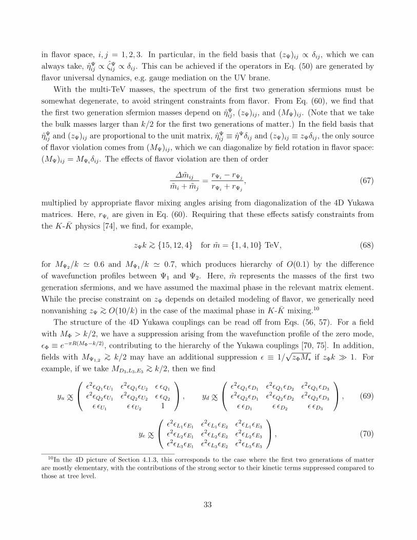
in flavor space, i, j = 1, 2, 3. In particular, in the field basis that (zΨ)ij ∝ δij, which we can
always take, ηΨij ∝ ζΨ
ij ∝ δij. This can be achieved if the operators in Eq. (50) are generated by
flavor universal dynamics, e.g. gauge mediation on the UV brane.
With the multi-TeV masses, the spectrum of the first two generation sfermions must be
somewhat degenerate, to avoid stringent constraints from flavor. From Eq. (60), we find that
the first two generation sfermion masses depend on ηΨij , (zΨ)ij, and (MΨ)ij. (Note that we take
the bulk masses larger than k/2 for the first two generations of matter.) In the field basis that
ηΨij and (zΨ)ij are proportional to the unit matrix, ηΨ
ij ≡ ηΨδij and (zΨ)ij ≡ zΨδij, the only source
of flavor violation comes from (MΨ)ij, which we can diagonalize by field rotation in flavor space:
(MΨ)ij = MΨiδij. The effects of flavor violation are then of order
∆mij
mi + mj
=rΨi − rΨj
rΨi + rΨj
, (67)
multiplied by appropriate flavor mixing angles arising from diagonalization of the 4D Yukawa
matrices. Here, rΨi are given in Eq. (60). Requiring that these effects satisfy constraints from
the K-K physics [74], we find, for example,
zΨk >∼ 15, 12, 4 for m = 1, 4, 10 TeV, (68)
for MΨ2/k ' 0.6 and MΨ1/k ' 0.7, which produces hierarchy of O(0.1) by the difference
of wavefunction profiles between Ψ1 and Ψ2. Here, m represents the masses of the first two
generation sfermions, and we have assumed the maximal phase in the relevant matrix element.
While the precise constraint on zΨ depends on detailed modeling of flavor, we generically need
nonvanishing zΨ>∼ O(10/k) in the case of the maximal phase in K-K mixing.10
The structure of the 4D Yukawa couplings can be read off from Eqs. (56, 57). For a field
with MΦ > k/2, we have a suppression arising from the wavefunction profile of the zero mode,
εΦ ≡ e−πR(MΦ−k/2), contributing to the hierarchy of the Yukawa couplings [70, 75]. In addition,
fields with MΨ1,2>∼ k/2 may have an additional suppression ε ≡ 1/
√zΦM∗ if zΦk 1. For
example, if we take MD3,L3,E3>∼ k/2, then we find
yu ∝∼
ε2εQ1εU1 ε2εQ1εU2 ε εQ1
ε2εQ2εU1 ε2εQ2εU2 ε εQ2
ε εU1 ε εU2 1
, yd ∝∼
ε2εQ1εD1 ε2εQ1εD2 ε2εQ1εD3
ε2εQ2εD1 ε2εQ2εD2 ε2εQ2εD3
ε εD1 ε εD2 ε εD3
, (69)
ye ∝∼
ε2εL1εE1 ε2εL1εE2 ε2εL1εE3
ε2εL2εE1 ε2εL2εE2 ε2εL2εE3
ε2εL3εE1 ε2εL3εE2 ε2εL3εE3
, (70)
10In the 4D picture of Section 4.1.3, this corresponds to the case where the first two generations of matterare mostly elementary, with the contributions of the strong sector to their kinetic terms suppressed compared tothose at tree level.
33

where O(1) factors are omitted in each element, and εΦ 1 only if πR(MΦ − k/2) 1 and
ε 1 only if zΦk 1. Therefore, with suitable choices for MΨi , the observed pattern of
the Yukawa couplings can be reproduced through physics of the bulk (i.e. the dynamics of the
strong sector in the 4D picture) while keeping approximate flavor universality for the first two
generation sfermion masses.
4.1.3 4D interpretation
Models discussed here can be interpreted as purely 4D models formulated in the conventional
grand desert, using the AdS/CFT correspondence. (For discussions on this correspondence, see
e.g. [59, 76].) In the 4D picture, the first two generations of matter are (mostly) elementary, while
the third generation quark-doublet and right-handed top multiplets arise as composite fields of
some strongly interacting sector, which exhibits nontrivial dynamics at an exponentially small
scale ≈ k′ = ke−πkR. (We mostly consider that the right-handed bottom and third-generation
lepton multiplets are elementary, although there is some flexibility on this choice.) This strong
dynamics also produces S, Hu, and Hd fields, together with superpotential interactions WH =
λSHuHd + f(S) at k′. (We focus on the case of IR-brane localized S in this section.) Since the
Higgs-top sector is strongly coupled at k′, the Landau pole constraint for the couplings in WH
(and the top Yukawa coupling) needs to be satisfied only below k′ [61], realizing the λSUSY
framework in Ref. [77].
Supersymmetry breaking is mediated at the scale Mmess, giving TeV to multi-TeV masses
to the elementary sfermions as well as the gauginos. The effect of supersymmetry breaking in
the composite sector is diluted by the near-conformal strong dynamics [62], as long as operators
associated with this effect have large anomalous dimensions [63]. This therefore yields only
negligible soft masses for the composite fields at k′.11 A composite field, however, may obtain
sizable supersymmetry breaking masses (only) if it mixes with an elementary state, which in the
5D picture corresponds to delocalizing the state from the IR brane.
The top Yukawa coupling is naturally large as the relevant fields are all composite. On the
other hand, the Yukawa couplings for the first two generations of matter are generated through
mixing of these states with fields in the composite sector, so are suppressed. The amount of
suppression depends on the dimension of the mixing operator, and thus varies field by field,
yielding a hierarchical pattern for the Yukawa matrices. Note that this way of dynamically
generating the Yukawa hierarchy does not contradict the stringent constraints on supersymmetric
flavor violation as long as supersymmetry breaking mediation at Mmess is flavor universal (e.g.
11In our models, supersymmetry breaking masses in the elementary sector, m ∼ a few TeV, is smaller than thecompositeness scale, k′ >∼ 10 TeV (see below). Therefore, the problem of a potentially large D-term operator [63],intrinsic to the framework of Refs. [62, 63, 64], does not arise, unless this operator is generated directly by thephysics at Mmess. The dilution of supersymmetry breaking effects in the composite sector has been studiedexplicitly in Ref. [65] in a setup similar to ours, using Seiberg duality.
34

Figure 15: The 4D interpretation of the models. The first two generations of matter are el-ementary, while the Higgs and top multiplets arise as composite states at the scale of strongdynamics, k′. The theory between k′ and TeV is λSUSY in Ref. [77] (with a modest Higgs-sectorcoupling λ), with light stops and left-handed sbottom.
as in the case of gauge mediation) and the contribution to the kinetic terms of the elementary
fields from the strong sector is small (which corresponds to the condition in Eq. (68) in 5D). The
overall picture for the 4D interpretation described here is depicted schematically in Fig. 15.
The value of the compositeness scale k′ is constrained by phenomenological considerations. As
in Eq. (64), we take the stops light to keep electroweak symmetry breaking natural. On the other
hand, the LHC bound on the gluino mass for these values of stop masses is mg>∼ 700 GeV, so
that we need a little “hierarchy” between mt and mg. Since mt receives a positive contribution
from mg through renormalization group evolution, this bounds the scale k′ from above. The
precise bound is (exponentially) sensitive to the low energy parameters, but we typically find
that k′ must be below an intermediate scale; in particular, it cannot be at the unification scale.
The value of k′ is also limited from above by Landau pole considerations for the couplings in
WH .
35

The lower bound on k′ can be obtained for a fixed mg by requiring that tL, tR, and bL
are sufficiently heavy to avoid the LHC bounds. Assuming that these states decay either into
the lightest neutralino or the gravitino within the detector, which we would need anyway to
avoid a strong constraint on quasi-stable stops, the masses of tL and bL must be larger than
about 250 GeV [58]. Moreover, if the neutralino to which these states decay is lighter than
≈ 100 GeV (or if they decay into the gravitino), then the mass of bL must be larger than about
400 GeV [78]. Since the running masses for these states, mQ3and mU3
, are vanishing at k′ (up
to small threshold corrections), this limits k′ from below for a fixed mg. In this paper, we take
k′ >∼ 10 TeV, (71)
so that the theory below the compositeness scale is the supersymmetric standard model with
the superpartner spectrum given by Eqs. (63 – 65). With these values of k′, other lower bounds
on k′ coming from precision electroweak measurements and flavor/CP violation induced by KK
excitations are satisfied [79]. (Note that the masses of the lowest KK excitations are given by
≈ πk′.)
Our models have the supersymmetric grand desert between k′ and k ∼ MPl. Thus, if the
strong sector respects a (global) unified symmetry, then we can discuss gauge coupling unifi-
cation, along the lines of Ref. [80]. The prediction depends on the location of matter fields,
especially D3, L3 and E3; in the minimal case where these fields have MΦ>∼ k/2, the three SM
gauge couplings approach at ∼ 1017 GeV, but with the precision of unification worse than that
in the SM (δg2/g2 ≈ 15% at the unification scale). We do not pursue the issue of unification
further in this paper.
4.2 Electroweak Symmetry Breaking
4.3 Overview
As outlined in Section 4.1.3, our theory above the compositeness scale k′ is SU(3)C ⊗SU(2)L⊗U(1)Y gauge theory that has the elementary fields Ψ1,2 (and D3, L3, E3) and the strongly inter-
acting near-conformal sector. The beta functions for the gauge group are given by
bA = bMSSMA − bQ3+U3+Hu,d
A + bCFT, (72)
where bCFT is the contribution from the strong sector, which corresponds to 1/g25Dk in the 5D
picture, and is universal if this sector respects a (global) unified symmetry. Supersymmetry
breaking masses for the elementary fields, including the gaugino masses MA, are generated at
Mmess, and they are evolved down to k′ by the renormalization group equations with Eq. (72).
The composite fields appear at k′, which have vanishing supersymmetry breaking masses at that
scale (up to small threshold corrections of O(M2A/16π2) in squared masses).
36

Physics of electroweak symmetry breaking is governed by the dynamics of the composite
sector and the gaugino masses. At scale k′, the strong sector produces the superpotential
WH = λSHuHd + f(S) + · · · , (73)
for the Higgs sector, where the dots represent higher dimension terms which are generically
suppressed by the warped-down cutoff scale M ′∗ = M∗e
−πkR. In case M ′∗ is close to the TeV
scale, these higher dimension terms could affect phenomenology; for example, the term (HuHd)2
can contribute to the Higgs boson mass [81]. Similarly, higher dimension terms in the Kahler
potential may affect phenomenology; for example, the terms S†HuHd and S†H†uQD can lead to
a µ term and down-type quark masses if S has an F -term expectation value.
In general, for relatively large values of k′ envisioned in Eq. (71), the effects of these higher
dimension operators are insignificant, except possibly for light quark/lepton masses. We there-
fore consider only renormalizable terms in the Higgs potential. In particular, in the rest of the
paper we focus on the case where WH contains only dimensionless terms in 4D, and discuss how
electroweak symmetry breaking can work in our models. In doing so, we assume
mQ3,U3,Hu,Hd≈ 0, (74)
at k′, i.e. we ignore possible threshold corrections at that scale, which are highly model-dependent.
(We later consider dynamics at the IR scale in which non-vanishing m2S is generated at k′ to
reproduce correct electroweak symmetry breaking.) This will illustrate basic features of elec-
troweak symmetry breaking in our framework, in the minimal setup.
4.3.1 Higgs sector: κSUSY
We consider a variant on the λSUSY model [77], which has the superpotential of the Next-to-
Minimal Supersymmetric Standard Model (NMSSM) form:
WH = λSHuHd +κ
3S3. (75)
To distinguish from other λSUSY studies in which the κ term does not play a dominant role, we
call this model κSUSY. We assume that S, Hu, and Hd are all localized to the IR brane, so we
require λ and κ to be perturbative only up to the scale k′, which we take to be 10 – 1000 TeV.
For k′ = 10 TeV, for example, we obtain λ(MZ) <∼ 1.8 for κ(MZ) = 0.7; for k′ = 1000 TeV,
λ(MZ) <∼ 1.1 for κ(MZ) = 0.7.
Because of Eq. (74), the only relevant dimensionful parameters for electroweak symmetry
breaking are the gaugino masses, except possibly for the supersymmetry breaking mass for
the S field (which we will introduce in the next subsection). They set the scale for the soft
37

supersymmetry breaking masses in the scalar potential
V = |λHuHd + κS2|2 + |λSHu|2 + |λSHd|2
+m2S|S|2 +m2
Hu|Hu|2 +m2Hd|Hd|2 + (λAλSHuHd −
κ
3AκS
3 + h.c.)
+g2
8(H†uσ
aHu +H†dσaHd)
2 +g′2
8(|Hu|2 − |Hd|2)2, (76)
through renormalization group evolution below k′. Successful electroweak symmetry breaking
requires all the S, Hu, and Hd fields to obtain vacuum expectation values, vs ≡ 〈S〉, vu ≡ 〈Hu〉,and vd ≡ 〈Hd〉.
Once the singlet has a vacuum expectation value, vs, we obtain µ = λvs and Bµ = λAλvs +
κλv2s = µ(Aλ+κµ/λ), where Bµ is the holomorphic supersymmetry breaking Higgs mass-squared.
We thus obtain the following Higgs mass-squared matrix (in the hu-hd-s basis):
M2scalar ≡ 1
2∂2V∂vi∂vj
= 12
(∂2V∂vi∂vj
− δij 1vi
∂V∂vi
)= 1
2×
g2v2
u + 2Bµtanβ
(4λ2 − g2)vuvd − 2Bµ 4µvu
(λ− κ
tanβ− λAλ
2µ tanβ
)(4λ2 − g2)vuvd − 2Bµ g2v2
d + 2Bµ tan β 4µvd
(λ− κ tan β − λAλ tanβ
2µ
)4µvu
(λ− κ
tanβ− λAλ
2µ tanβ
)4µvd
(λ− κ tan β − λAλ tanβ
2µ
)8κBµλ
(1− µ(Aλ+Aκ
4 )Bµ
+ λ3Aλvuvd4κµBµ
) ,
(77)
where g2 ≡ g2 +g′2, and we have assumed that all three expectation values are real and nonzero.
For us, the Aλ and Aκ terms are small because they are generated essentially only through weak
renormalization group evolution below k′; |Aλ,κ| <∼ O(10 GeV). Other than contributing to Bµ,
they also contribute to singlet-doublet mixing and pseudoscalar masses, but we will ignore them
in the following discussion on the (non-pseudo)scalar spectrum, as the result is not very sensitive
to the values of such small A terms.
We now discuss important differences between κSUSY and the MSSM as well as previous
λSUSY/NMSSM studies [52, 82, 83]. They are illustrated in Fig. 16, where (tree-level) scalar
masses are plotted as a function of λ for sample values of tan β, κ, µ.
• We see that κ plays a crucial role in this theory because it appears in Bµ ⊃ κµ2/λ. It
determines the degree of decoupling of the SM-like Higgs from the heavier scalars. The
limit κ = 0 leads to nearly massless modes and is therefore unacceptable. In fact, as we
shall see, we need κ ∼ λ for a successful theory of electroweak symmetry breaking.
• The new quartic term λ2|HuHd|2 leads to an extra doublet-doublet mixing which competes
against Bµ: M212 = (2λ2− g2/2)vuvd−Bµ. As long as 2λ2vuvd < Bµ + g2vuvd/2, this leads
to the well-known enhancement of the Higgs mass in λSUSY, see Eq. (78). However, once
38

0.5 1.0 1.5 2.0Λ
100
200
300
400
500
600
700GeV
Scalar Masses
(a) tanβ = 1.2, κ = 1.0, µ = 200 GeV
0.5 1.0 1.5 2.0Λ
100
200
300
400
500
600
700GeV
Scalar Masses
(b) tanβ = 2.0, κ = 1.0, µ = 200 GeV
Figure 16: Two representative plots of the scalar mass spectrum in κSUSY. The solid (black),dot-dashed (red), and dashed (blue) lines represent the masses of the three mass eigenstates,which at small λ correspond to the SM, heavy-doublet, and singlet like Higgs bosons, respectively.The horizontal (yellow) line shows mh = 125 GeV, and the dotted (violet) line is the mass ofthe lightest Higgs boson with singlet-doublet mixing turned off by hand. In the left figure wesee that λ-doublet mixing is responsible for lowering the mass of the Higgs below its decouplinglimit, Eq. (78), rather than doublet-singlet mixing. This is a generic feature for tan β ∼ 1. Inthe right figure, we see that as we increase tan β, singlet-doublet mixing sets in at lower λ thandoublet-doublet mixing but that both are important in lowering the Higgs mass below Eq. (78).
2λ2vuvd > Bµ + g2vuvd/2, the absolute magnitude of the off-diagonal term now increases
with λ which leads to lowering of the Higgs mass through the very same term. We call this
effect λ-doublet mixing. We find that in κSUSY, this is the main effect that lowers the Higgs
mass at large λ and small tan β, rather than mixing with the singlet, see Fig. 16. This is
different from Ref. [52], whose potential contains multiple extra free scales (Bµ, the singlet
mass) which are potentially large. (Their benchmark point has Bµ ≈ 4µ2 = (400 GeV)2.
In this region, λ-doublet mixing accounts for only 15% of the lowering of the Higgs mass
below its decoupling limit, Eq. (78); the rest comes from singlet-doublet mixing.) In fact,
in κSUSY, λ ∼ 2 is excluded for µ ∼ 200 GeV exactly for this reason: the Higgs becomes
tachyonic (i.e. the correct electroweak symmetry breaking vacuum disappears).
• The mass of the singlet-like scalar is not really a free parameter. It decouples together with
the heavy Higgs (Bµ →∞) but not independently. This kind of relation is to be expected
in a model with a scale-free superpotential, with λ ∼ κ. It is simply an accidental feature
(due to the coefficient in M233) that the singlet-like scalar is heavier than other scalars by
a factor of a few, in the limit of no mixing and λ ∼ κ.
39

• Doublet-singlet mixing now depends on a difference between λ and κ. We find that,
although the singlet-like Higgs is not very heavy, this greatly reduces mixing of the Higgs
doublet component with the singlet and can lead to decoupling of the SM-like Higgs from
the singlet for singlet masses as low as 400 GeV for tan β ∼ 1.
In the limit of small λ-doublet mixing (2λ2vuvd < Bµ + g2vuvd/2) and negligible doublet-
singlet mixing, the tree-level mass of the SM-like Higgs boson is given by
m2h ≈M2
Z cos22β + λ2v2 sin22β. (78)
In the appendix, we present analytical formulae for mh that include both large λ-doublet and
singlet-doublet mixings up to second order in an expansion in m2h/m
2H (light Higgs mass over
heavy Higgs mass); we also present the exact solution to mh in the regime where λ-doublet
mixing dominates over doublet-singlet mixing as well as in the opposite case.
In Fig. 17(a), we present contours of the lightest Higgs boson mass, mh, for typical values of
parameters, where we have added the one-loop top-stop contribution with mt = 450 GeV and
At = 0. In Fig. 17(b), we show contours of the charged Higgs boson mass, which is given by
m2H+ =
2Bµ
sin 2β− λ2v2 +M2
W . (79)
In the non-decoupling region (Bµ/v2 >∼ 1) and for λ >
√2/ sin 2β, the charged Higgs boson can
become tachyonic. On the other hand, its mass cannot significantly fall below 300 GeV due to
constraints from b → sγ. This provides an important constraint on our parameter space and
forces us to choose relatively low values of λ <∼ 1.
Another potential issue is a light pseudoscalar arising from an approximateR symmetry under
which S,Hu, Hd have a charge of 2/3. This symmetry is spontaneously broken by vs, vu, vd so
that there is a light R-axion. This axion obtains a mass through loops of gauginos, mixing with
other axions, such as the QCD axion, and Aλ, Aκ. In Ref. [84], it was determined that the A
terms provide the dominant contribution for 10−3 <∼ |Aλ,κ|/v 1, which we satisfy. The mass
of the R-axion due to the A terms is given in terms of an expansion in Aλ,κ/v by
m2A1≈ 9
µ
λ
(λAλ
2
cos2θAsin 2β
+κAκ
3sin2θA
)+O(A2
λ,κ), (80)
where tan θA = µ/(λv sin 2β) +O(Aλ,κ/v). We see that the mass is the geometric mean of µ and
Aλ,κ times O(1) factors. Since we generically have |Aλ| > 1 GeV, the mass is in tens of GeVs,
so we are safe from the constraint from Υ decays. Since λ, κ are O(1), however, the Higgs can
also decay into the R-axion with a large branching fraction, if this decay mode is kinematically
allowed. Assuming mh = 125 GeV, we find that this happens for |Aλ| < 10 GeV (neglecting
Aκ). Depending on parameters, we can have |Aλ| >∼ 10 GeV, in which case decays of the lightest
Higgs boson are SM-like.
40
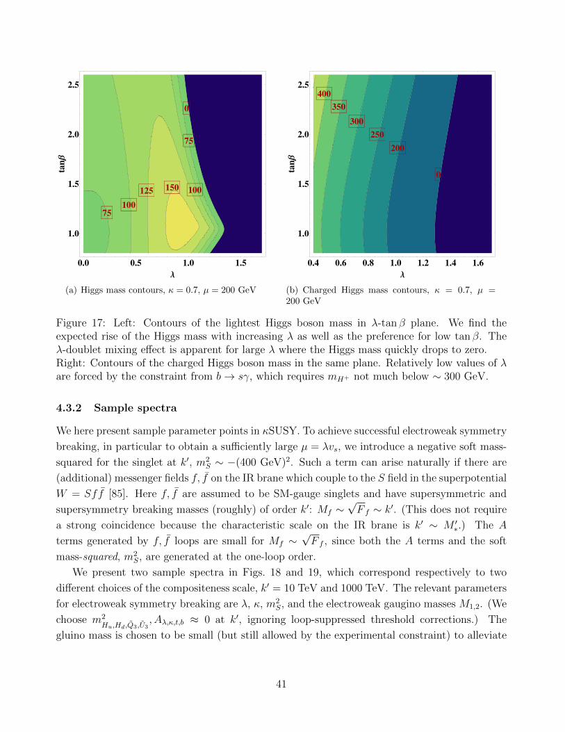
0
75
75
100
100
125150
0.0 0.5 1.0 1.5
1.0
1.5
2.0
2.5
Λ
tanΒ
(a) Higgs mass contours, κ = 0.7, µ = 200 GeV
0
200
250
300
350
400
0.4 0.6 0.8 1.0 1.2 1.4 1.6
1.0
1.5
2.0
2.5
Λ
tanΒ
(b) Charged Higgs mass contours, κ = 0.7, µ =200 GeV
Figure 17: Left: Contours of the lightest Higgs boson mass in λ-tan β plane. We find theexpected rise of the Higgs mass with increasing λ as well as the preference for low tan β. Theλ-doublet mixing effect is apparent for large λ where the Higgs mass quickly drops to zero.Right: Contours of the charged Higgs boson mass in the same plane. Relatively low values of λare forced by the constraint from b→ sγ, which requires mH+ not much below ∼ 300 GeV.
4.3.2 Sample spectra
We here present sample parameter points in κSUSY. To achieve successful electroweak symmetry
breaking, in particular to obtain a sufficiently large µ = λvs, we introduce a negative soft mass-
squared for the singlet at k′, m2S ∼ −(400 GeV)2. Such a term can arise naturally if there are
(additional) messenger fields f, f on the IR brane which couple to the S field in the superpotential
W = Sff [85]. Here f, f are assumed to be SM-gauge singlets and have supersymmetric and
supersymmetry breaking masses (roughly) of order k′: Mf ∼√F f ∼ k′. (This does not require
a strong coincidence because the characteristic scale on the IR brane is k′ ∼ M ′∗.) The A
terms generated by f, f loops are small for Mf ∼√F f , since both the A terms and the soft
mass-squared, m2S, are generated at the one-loop order.
We present two sample spectra in Figs. 18 and 19, which correspond respectively to two
different choices of the compositeness scale, k′ = 10 TeV and 1000 TeV. The relevant parameters
for electroweak symmetry breaking are λ, κ, m2S, and the electroweak gaugino masses M1,2. (We
choose m2Hu,Hd,Q3,U3
, Aλ,κ,t,b ≈ 0 at k′, ignoring loop-suppressed threshold corrections.) The
gluino mass is chosen to be small (but still allowed by the experimental constraint) to alleviate
41

fine-tuning, and the bino is chosen to be the lightest observable-sector supersymmetric particle
(LOSP). For the gluino mass we add the one-loop threshold correction, which can be as large
as ≈ 20% for the multi-TeV squark masses [86]. In this section, we assume that the gravitino
is heavier than the LOSP, so that the bino is the lightest supersymmetric particle. This is the
case for Mmess>∼ MPl, or for Mmess
<∼ MPl if there is additional supersymmetry breaking that
does not contribute to the MSSM superparticle masses but pushes up the gravitino mass above
the LOSP mass [87]. If the gravitino is lighter than the bino, somewhat stronger bounds on the
gluino mass would apply [88]. For example, if the bino decays promptly to the gravitino, then
the lower bound is mg ≈ 900 GeV, instead of ≈ 700 GeV.
In presenting the sample points, we also evaluate the amount of fine-tuning, adopting a
conventional criterion [89]
∆ = maxi,j
d lnAid lnBj
, (81)
where Ai = (m2h, v
2) and Bj are UV parameters to be specified below. The Ai correspond
to the (θh,hu vu + θh,hd vd + θh,svs) and (~vu + ~vd)/v directions in the three-dimensional vu, vd, vs
space, respectively, where we define scalar mixing angles in terms of eigenvector overlap: h =
θh,huhu+θh,hdhd+θh,ss. In the case of λ-doublet or singlet-doublet mixing, fine-tuning (e.g. due to
stops) may be much alleviated compared to the MSSM due to level repulsion which is generated
naturally through large off-diagonal elements in the mass matrix; in the case of singlet-doublet
mixing, this has been analyzed in Ref. [52]. We here point out that large-mixing, natural scenar-
ios with TeV-scale stops are typically accompanied by drastic deviations of Higgs couplings, so
if the Higgs has only moderate deviations from SM cross sections and decay rates, then natural-
ness generically requires light stops. In our analysis, we choose Bj = (λ, κ,m2S,M1,2,3, k
′, yt, m).
3.4.2.1 k′ = 10 TeV
The following considerations give a bottom-up picture of what is needed to generate a natural
superpartner spectrum (in the decoupling regime) [90, 58] that radiatively breaks electroweak
symmetry with k′ = 10 TeV:
• The fine-tuning constraint (∆−1 >∼ 20%) requires |µ| <∼ 210 GeV, mt<∼ 410 GeV (for
degenerate stop masses without mixing), mg<∼ 790 GeV (at the leading-log level; the actual
bound is significantly weaker because of the effect of strong interactions), mW<∼ 890 GeV,
mB<∼ 2800 GeV, and m <∼ 4 TeV.
• Electroweak symmetry breaking requires λ, κ ∼ 0.7 at low energies, as discussed in the last
section; we also need m2S ∼ −(400 GeV)2 to generate a sufficiently large µ term.
In Fig. 18, we show a typical mass spectrum for k′ = 10 TeV, where the lightest Higgs boson
mass is evaluated with the one-loop top-stop contribution added. The production cross section
42

Figure 18: A typical mass spectrum for a compositeness scale of k′ = 10 TeV. The stateswith mixing are labeled by their largest components. In the left diagram, the states are alwaysordered from heavy to light. The gluino mass of mg = 946 GeV in the table corresponds toM3 = 801 GeV at the scale mt obtained using the MSSM renormalization group evolution.The wino is relatively heavy, which is necessary to generate a mass for the light pseudoscalarmAs > mh/2 through the Aλ term, in line with recent hints of a Higgs discovery. If the wino ismuch lighter, the Higgs would decay almost entirely to pseudoscalars.
σ(gg → h) is modified relative to the SM due to non-decoupling stop contributions and A terms;
this sample point has an enhancement of 13%. Unlike in the MSSM, the decay rate of the Higgs
into bb is depleted in λSUSY relative to the SM rate. As expanded in m2h/m
2H , the rate is given
by (see the appendix)
Γ(h→ bb)
ΓSM(h→ bb)= 1− tan β sin22β
λv√|λ2v2 −M2
Z |2Bµ
. (82)
For the k′ = 10 TeV spectrum, this formula gives 0.88, within 10% of the exact result, 0.96.
Because of this suppression, the branching ratios into other modes are enhanced. In particular,
we find that Br(h→ γγ) is increased by 4% with respect to the SM, resulting in an enhancement
of σ(gg → h) × Br(h → γγ) of 18%. This effect of an enhanced γγ signal has been observed
for a different parameter space of λSUSY in Ref. [52]; however, here the effect is not large and
the decays are practically SM-like. Notice in particular the small mixing of the Higgs with the
43

Figure 19: A typical mass spectrum for a compositeness scale of k′ = 1000 TeV. Definitions areas in Fig. 18. The gluino mass of mg = 814 GeV corresponds to M3 = 710 GeV at the scale mt
obtained using the MSSM renormalization group evolution.
singlet as anticipated in section 4.3.1. For our k′ = 10 TeV point, decay rate times branching
ratio of both the heavy Higgs and the singlet into WW or ZZ is four orders of magnitude below
that of the SM Higgs of the same mass, which makes them invisible to SM Higgs searches. For
the fine-tuning parameter, we obtain ∆−1 = 19%, consistent with expectations based on the
general argument.
The heavy Higgs decays into AsAs, AsZ, and tt, with As decaying predominantly into bb. The
singlet decays into AsAs, AsZ, tt, and h+h−. Due to associated Z production, discovery of these
particles may be possible at e+e− colliders such as the ILC/CLIC.
3.4.2.2 k′ = 1000 TeV
The fine-tuning constraint will be more severe for k′ = 1000 TeV than for k′ = 10 TeV
because of the large ln(k′/TeV) = 6.9. Performing the same bottom-up analysis as in the case
of k′ = 10 TeV, we find:
• The fine-tuning constraint (∆−1 >∼ 10%) requires |µ| <∼ 290 GeV, mt<∼ 370 GeV (for
degenerate stop masses without mixing), mg<∼ 460 GeV (again at the leading-log level),
mW<∼ 800 GeV, mB
<∼ 2500 GeV, and m <∼ 3.6 TeV.
For k′ = 1000 TeV, the theory is expected to be fine-tuned at the 10% level.
44

In Fig. 19, we show a typical mass spectrum for k′ = 1000 TeV. We find that, as in the
k′ = 10 TeV case, the phenomenology of the Higgs is mostly SM-like: the production cross
section σ(gg → h) is enhanced by 9% relative to the SM; Eq. (82) gives 0.92 as the decay rate of
the Higgs to bb with respective to the SM, whereas the exact result is 0.96. This translates into
an increase of σ(gg → h)× Br(h→ γγ) of 13% with respect to the SM. As for the heavy Higgs
or the singlet, we again find four orders of magnitude suppression of production cross section
times branching ratio into WW or ZZ compared to the SM Higgs with the same mass. We find
fine-tuning of ∆−1 = 10% for this sample point, which is in agreement with expectations.
We find that if we relax our requirement of tuning slightly, we can choose k′ to be much larger
than 1000 TeV without conflicting with Landau pole constraints. We, however, note that two-
loop stop contributions to the Higgs quartic are negative and the theory will therefore require
larger λ, κ, so it is not obvious that this statement will hold at two loops. Using the tree-level
potential as the other extreme to the one-loop potential, one finds that large λ, κ ∼ 0.8 – 0.9 are
needed to push the Higgs mass high enough and one cannot take k′ much higher than 1000 TeV
due to Landau pole constraints. The truth is expected to lie somewhere between the tree-level
and one-loop situations.
4.4 Flat Space Realization
We now discuss realizing our basic setup, Fig. 1, using a flat space extra dimension. An obvious
way to do this is to simply turn off the curvature in models of Section 4.1. The analysis then
goes similarly with the replacement k′ → 1/πR, except that we now do not have a large desert
above the compactification scale, 1/R, so we cannot have the high-scale see-saw mechanism or
conventional gauge coupling unification.
In this section, we pursue an alternative realization, adopting supersymmetry breaking by
boundary conditions associated with a compact extra dimension [91]. Our model is essentially
that in Ref. [92]. Specifically, we consider an SU(3)C⊗SU(2)L⊗U(1)Y gauge theory in 5D, with
the extra dimension compactified on S1/Z2: 0 ≤ y ≤ πR. We introduce three generations of
matter and Higgs fields in the bulk, but localize the third-generation quark doublet, right-handed
top, and Higgs multiplets to the y = πR brane:
MQ3,U3,Hu,Hd −1
πR, (83)
where MΦ represents bulk masses as in previous sections. When supersymmetry is broken by
twisted boundary conditions with twist parameter α, we obtain
mQ3,U3,Hu,Hd mΨ1,2,D3,L3,E3
=α
R, (84)
45

at the scale 1/R, where we have taken
|MΨ1,2,D3,L3,E3| 1
πR. (85)
This condition guarantees that the first two generation sfermions are nearly degenerate in mass,
avoiding stringent constraints from flavor violation.
To obtain the spectrum we want, we take α/R to be in the multi-TeV region. For the gauge
multiplets, we introduce sizable gauge kinetic terms on (one or both of) branes, which control
the size of the gaugino masses:
MA =πRg2
4,A
g25,A
α
R, (86)
where g5,A and g4,A are the 5D bulk and 4D gauge couplings, respectively, with g4,A given by
1
g24,A
=πR
g25,A
+1
g20,A
+1
g2π,A
, (87)
in terms of g5,A and the brane-localized gauge couplings at y = 0 and πR, g0,A and gπ,A. We
take MA to be in the sub-TeV region.
Introducing a singlet field S together with the superpotential λSHuHd+f(S) on the y = πR
brane, the analysis of electroweak symmetry breaking goes as in the previous section, with the
identification
k′ → 1
πR, m→ α
R. (88)
A negative soft mass-squared for S can be induced, for example, by introducing some bulk field
that has a Yukawa coupling to S on the y = πR brane.
In the present model, the two circles in Fig. 1 are interpreted as the 5D bulk (left) and the
y = πR brane (right), rather than the y = 0 and πR branes as in previous models. Because of
Eq. (85), only a part of the Yukawa hierarchy can be explained by wavefunction profiles. With
Eqs. (83, 85) the Yukawa matrices obtain the following structure from the wavefunctions:
yu ∼
ε2 ε2 εε2 ε2 εε ε 1
, yd ∼
ε2 ε2 ε2
ε2 ε2 ε2
ε ε ε
, ye ∼
ε2 ε2 ε2
ε2 ε2 ε2
ε2 ε2 ε2
, (89)
where O(1) factors are omitted in each element, and ε ≡ 1/√πR is the volume dilution factor.
The structure beyond this must come from that of 5D Yukawa couplings between matter and
Higgs on the y = πR brane.
4.5 Conclusions
In this paper we have presented supersymmetric models in which light stops are obtained while
keeping near flavor degeneracy for the first two generation sfermions. Such a spectrum is mo-
tivated by the naturalness argument together with the recent LHC data. Our construction is
46

based on the basic picture in Fig. 1: being “close to” electroweak symmetry breaking implies
being “away from” supersymmetry breaking, and vice versa. In models where the two sectors
correspond to the two branes at the opposite ends of a (warped or flat) extra dimension, the de-
sired superpartner spectra are obtained while reproducing the hierarchy in the Yukawa matrices
through wavefunction profiles of the quark/lepton fields. A relatively large Higgs boson mass,
including mh = 125 GeV, can be easily accommodated if the scale of Kaluza-Klein excitations is
low. For models in warped space, the AdS/CFT correspondence allows us to interpret them in
terms of purely 4D theories in which the top and Higgs (and the left-handed bottom) multiplets
are composites of some strongly interacting sector. An alternative realization of the picture in
Fig. 1 is obtained by identifying the two sectors as the bulk of a flat extra dimension and a brane
on its boundary, and by breaking supersymmetry by boundary conditions, which we have also
discussed.
In the coming years, the LHC will be exploring the parameter regions of supersymmetric
theories in which the stops (and the left-handed sbottom) are light. If electroweak symmetry
breaking is indeed natural in the conventional sense, the LHC will find the stops in the sub-TeV
region. If not, and if the SM-like Higgs boson is confirmed with mh ' 125 GeV, then we would
be led to consider that supersymmetry is absent at low energies, or it is realized in a somewhat
fine-tuned form, perhaps along the lines of scenarios considered in Refs. [93, 94, 95].
References
[1] ATLAS Collaboration, ATLAS-CONF-2012-019.
[2] CMS Collaboration, CMS-PAS-HIG-12-008.
[3] A. Djouadi, Phys. Rept. 459, 1 (2008) [hep-ph/0503173].
[4] P. Draper, P. Meade, M. Reece and D. Shih, arXiv:1112.3068 [hep-ph].
[5] L. J. Hall, D. Pinner and J. T. Ruderman, JHEP 1204, 131 (2012) [arXiv:1112.2703 [hep-
ph]].
[6] R. Barbieri, L. J. Hall, Y. Nomura and V. S. Rychkov, Phys. Rev. D 75, 035007 (2007)
[hep-ph/0607332].
[7] R. Harnik, G. D. Kribs, D. T. Larson and H. Murayama, Phys. Rev. D 70, 015002 (2004)
[hep-ph/0311349].
[8] U. Ellwanger, C. Hugonie and A. M. Teixeira, Phys. Rept. 496, 1 (2010) [arXiv:0910.1785
[hep-ph]].
47

[9] P. Batra, A. Delgado, D. E. Kaplan and T. M. P. Tait, JHEP 0402, 043 (2004) [hep-
ph/0309149].
[10] A. Maloney, A. Pierce and J. G. Wacker, JHEP 0606, 034 (2006) [hep-ph/0409127].
[11] P. W. Graham, A. Ismail, S. Rajendran and P. Saraswat, Phys. Rev. D 81, 055016 (2010)
[arXiv:0910.3020 [hep-ph]].
[12] S. P. Martin, Phys. Rev. D 81, 035004 (2010) [arXiv:0910.2732 [hep-ph]].
[13] U. Ellwanger, JHEP 1203, 044 (2012) [arXiv:1112.3548 [hep-ph]].
[14] A. Arvanitaki and G. Villadoro, JHEP 1202, 144 (2012) [arXiv:1112.4835 [hep-ph]].
[15] M. Endo, K. Hamaguchi, S. Iwamoto, K. Nakayama and N. Yokozaki, arXiv:1112.6412
[hep-ph].
[16] ATLAS Collaboration, ATLAS-CONF-2012-007.
[17] T. Appelquist, B. A. Dobrescu and A. R. Hopper, Phys. Rev. D 68, 035012 (2003) [hep-
ph/0212073].
[18] K. Intriligator and M. Sudano, JHEP 1006, 047 (2010) [arXiv:1001.5443 [hep-ph]].
[19] M. Buican and Z. Komargodski, JHEP 1002, 005 (2010) [arXiv:0909.4824 [hep-ph]].
[20] E. Salvioni, G. Villadoro and F. Zwirner, JHEP 0911, 068 (2009) [arXiv:0909.1320 [hep-
ph]].
[21] M. S. Carena, J. R. Espinosa, M. Quiros and C. E. M. Wagner, Phys. Lett. B 355, 209
(1995) [hep-ph/9504316].
[22] G. Cacciapaglia, C. Csaki, G. Marandella and A. Strumia, Phys. Rev. D 74, 033011 (2006)
[hep-ph/0604111].
[23] E. Accomando, A. Belyaev, L. Fedeli, S. F. King and C. Shepherd-Themistocleous, Phys.
Rev. D 83, 075012 (2011) [arXiv:1010.6058 [hep-ph]].
[24] S. Weinberg, Phys. Rev. Lett. 59, 2607 (1987).
[25] A. H. Guth and E. J. Weinberg, Nucl. Phys. B 212, 321 (1983); A. Vilenkin, Phys. Rev.
D 27, 2848 (1983); A. D. Linde, Phys. Lett. B 175, 395 (1986); Mod. Phys. Lett. A 1, 81
(1986).
48

[26] R. Bousso and J. Polchinski, JHEP 06, 006 (2000) [arXiv:hep-th/0004134]; S. Kachru,
R. Kallosh, A. Linde and S. P. Trivedi, Phys. Rev. D 68, 046005 (2003) [arXiv:hep-
th/0301240]; L. Susskind, arXiv:hep-th/0302219; M. R. Douglas, JHEP 05, 046 (2003)
[arXiv:hep-th/0303194].
[27] For reviews, see e.g. A. H. Guth, Phys. Rept. 333, 555 (2000) [arXiv:astro-ph/0002156];
A. Vilenkin, J. Phys. A 40, 6777 (2007) [arXiv:hep-th/0609193]; S. Winitzki, Lect. Notes
Phys. 738, 157 (2008) [arXiv:gr-qc/0612164]; A. Linde, Lect. Notes Phys. 738, 1 (2008)
[arXiv:0705.0164 [hep-th]].
[28] Y. Nomura, arXiv:1104.2324 [hep-th].
[29] H. Martel, P. R. Shapiro and S. Weinberg, Astrophys. J. 492, 29 (1998) [arXiv:astro-
ph/9701099]; G. Efstathiou, Mon. Not. Roy. Astron. Soc. 274, L73 (1995).
[30] J. Garriga, M. Livio and A. Vilenkin, Phys. Rev. D 61, 023503 (2000) [arXiv:astro-
ph/9906210]; L. Pogosian and A. Vilenkin, JCAP 01, 025 (2007) [arXiv:astro-ph/0611573].
[31] R. Bousso, R. Harnik, G. D. Kribs and G. Perez, Phys. Rev. D 76, 043513 (2007) [arXiv:hep-
th/0702115]; J. M. Cline, A. R. Frey and G. Holder, Phys. Rev. D 77, 063520 (2008)
[arXiv:0709.4443 [hep-th]].
[32] A. De Simone, A. H. Guth, M. P. Salem and A. Vilenkin, Phys. Rev. D 78, 063520 (2008)
[arXiv:0805.2173 [hep-th]].
[33] R. Bousso, L. J. Hall and Y. Nomura, Phys. Rev. D 80, 063510 (2009) [arXiv:0902.2263
[hep-th]].
[34] M. P. Salem, Phys. Rev. D 80, 023502 (2009) [arXiv:0902.4485 [hep-th]]; R. Bousso and
S. Leichenauer, Phys. Rev. D 81, 063524 (2010) [arXiv:0907.4917 [hep-th]]; R. Bousso,
B. Freivogel, S. Leichenauer and V. Rosenhaus, arXiv:1012.2869 [hep-th].
[35] R. Bousso and L. Susskind, arXiv:1105.3796 [hep-th].
[36] E. Komatsu et al. [WMAP Collaboration], Astrophys. J. Suppl. 192, 18 (2011)
[arXiv:1001.4538 [astro-ph.CO]].
[37] R. Bousso, B. Freivogel and I. S. Yang, Phys. Rev. D 79, 063513 (2009) [arXiv:0808.3770
[hep-th]].
[38] W. H. Press and P. Schechter, Astrophys. J. 187, 425 (1974).
[39] C. Lacey and S. Cole, Mon. Not. Roy. Astron. Soc. 262, 627 (1993).
49

[40] G. Kauffmann et al. [SDSS Collaboration], Mon. Not. Roy. Astron. Soc. 341, 54 (2003)
[arXiv:astro-ph/0205070].
[41] M. Tegmark, A. Aguirre, M. J. Rees and F. Wilczek, Phys. Rev. D 73, 023505 (2006)
[arXiv:astro-ph/0511774].
[42] A. Cattaneo, A. Dekel, J. Devriendt, B. Guiderdoni and J. Blaizot, Mon. Not. Roy. Astron.
Soc. 370, 1651 (2006) [arXiv:astro-ph/0601295].
[43] C. H. Lineweaver, Icarus 151, 307 (2001) [arXiv:astro-ph/0012399].
[44] D. A. Fischer and J. Valenti, Astrophys. J. 622, 1102 (2005); D. Grether and
C. H. Lineweaver, Astrophys. J. 669, 1220 (2007).
[45] R. Maiolino et al., Astron. Astrophys. 488, 463 (2008) [arXiv:0806.2410 [astro-ph]];
P. S. Behroozi, C. Conroy and R. H. Wechsler, Astrophys. J. 717, 379 (2010) [arXiv:1001.0015
[astro-ph.CO]].
[46] M. Tegmark and M. J. Rees, Astrophys. J. 499, 526 (1998) [arXiv:astro-ph/9709058].
[47] J. A. Peacock, Mon. Not. Roy. Astron. Soc. 379, 1067 (2007) [arXiv:0705.0898 [astro-ph]].
[48] R. Bousso and S. Leichenauer, Phys. Rev. D 79, 063506 (2009) [arXiv:0810.3044 [astro-ph]].
[49] O. Lahav, P. B. Lilje, J. R. Primack and M. J. Rees, Mon. Not. Roy. Astron. Soc. 251, 128
(1991).
[50] G. Aad et al. [ATLAS Collaboration], arXiv:1109.6572 [hep-ex].
[51] ATLAS report, ATLAS-CONF-2011-163; CMS report, CMS-PAS-HIG-11-032.
[52] L. J. Hall, D. Pinner and J. T. Ruderman, arXiv:1112.2703 [hep-ph].
[53] M. Dine, A. Kagan and S. Samuel, Phys. Lett. B 243, 250 (1990).
[54] S. Dimopoulos and G. F. Giudice, Phys. Lett. B 357, 573 (1995) [hep-ph/9507282]; A. Po-
marol and D. Tommasini, Nucl. Phys. B 466, 3 (1996) [hep-ph/9507462]; A. G. Cohen,
D. B. Kaplan and A. E. Nelson, Phys. Lett. B 388, 588 (1996) [hep-ph/9607394].
[55] P. Binetruy and E. Dudas, Phys. Lett. B 389, 503 (1996) [arXiv:hep-th/9607172]; G. Dvali
and A. Pomarol, Phys. Rev. Lett. 77, 3728 (1996) [arXiv:hep-ph/9607383]; J. Hisano,
K. Kurosawa and Y. Nomura, Phys. Lett. B 445, 316 (1999) [hep-ph/9810411]; Nucl. Phys.
B 584, 3 (2000) [hep-ph/0002286].
50

[56] For recent work, see e.g. N. Craig, D. Green and A. Katz, JHEP 07, 045 (2011)
[arXiv:1103.3708 [hep-ph]]. R. Barbieri, G. Isidori, J. Jones-Perez, P. Lodone and
D. M. Straub, Eur. Phys. J. C 71, 1725 (2011) [arXiv:1105.2296 [hep-ph]]; R. Essig, E. Iza-
guirre, J. Kaplan and J. G. Wacker, JHEP 01, 074 (2012) [arXiv:1110.6443 [hep-ph]];
R. Auzzi, A. Giveon and S. B. Gudnason, arXiv:1112.6261 [hep-ph].
[57] C. Brust, A. Katz, S. Lawrence and R. Sundrum, arXiv:1110.6670 [hep-ph].
[58] M. Papucci, J. T. Ruderman and A. Weiler, arXiv:1110.6926 [hep-ph].
[59] R. Contino, Y. Nomura and A. Pomarol, Nucl. Phys. B 671, 148 (2003) [hep-ph/0306259];
G. Burdman and Y. Nomura, Phys. Rev. D 69, 115013 (2004) [hep-ph/0312247]; Y. Nomura,
hep-ph/0410348.
[60] J. Erlich, E. Katz, D. T. Son and M. A. Stephanov, Phys. Rev. Lett. 95, 261602 (2005) [hep-
ph/0501128]; L. Da Rold and A. Pomarol, Nucl. Phys. B 721, 79 (2005) [hep-ph/0501218].
[61] A. Birkedal, Z. Chacko and Y. Nomura, Phys. Rev. D 71, 015006 (2005) [hep-ph/0408329].
[62] T. Gherghetta and A. Pomarol, Phys. Rev. D 67, 085018 (2003) [hep-ph/0302001].
[63] R. Sundrum, JHEP 01, 062 (2011) [arXiv:0909.5430 [hep-th]].
[64] T. Gherghetta, B. von Harling and N. Setzer, JHEP 07, 011 (2011) [arXiv:1104.3171 [hep-
ph]].
[65] C. Csaki, L. Randall and J. Terning, arXiv:1201.1293 [hep-ph].
[66] N. Craig, M. McCullough and J. Thaler, arXiv:1201.2179 [hep-ph].
[67] S. Krippendorf, H. P. Nilles, M. Ratz and M. W. Winkler, arXiv:1201.4857 [hep-ph].
[68] L. Randall and R. Sundrum, Phys. Rev. Lett. 83, 3370 (1999) [hep-ph/9905221].
[69] D. Marti and A. Pomarol, Phys. Rev. D 64, 105025 (2001) [hep-th/0106256]; N. Arkani-
Hamed, T. Gregoire and J. Wacker, JHEP 03, 055 (2002) [hep-th/0101233].
[70] T. Gherghetta and A. Pomarol, Nucl. Phys. B 586, 141 (2000) [arXiv:hep-ph/0003129].
[71] Y. Nomura, JHEP 11, 050 (2003) [hep-ph/0309189].
[72] Y. Grossman and M. Neubert, Phys. Lett. B 474, 361 (2000) [hep-ph/9912408].
[73] G. F. Giudice, M. Nardecchia and A. Romanino, Nucl. Phys. B 813, 156 (2009)
[arXiv:0812.3610 [hep-ph]].
51

[74] See, e.g., F. Gabbiani, E. Gabrielli, A. Masiero and L. Silvestrini, Nucl. Phys. B 477, 321
(1996) [hep-ph/9604387]; K. Blum, Y. Grossman, Y. Nir and G. Perez, Phys. Rev. Lett. 102,
211802 (2009) [arXiv:0903.2118 [hep-ph]].
[75] S. Hamidi and C. Vafa, Nucl. Phys. B 279, 465 (1987); L. E. Ibanez, Phys. Lett. B 181,
269 (1986); N. Arkani-Hamed and M. Schmaltz, Phys. Rev. D 61, 033005 (2000) [arXiv:hep-
ph/9903417].
[76] N. Arkani-Hamed, M. Porrati and L. Randall, JHEP 08, 017 (2001) [hep-th/0012148];
R. Rattazzi and A. Zaffaroni, JHEP 04, 021 (2001) [hep-th/0012248].
[77] R. Barbieri, L. J. Hall, Y. Nomura and V. S. Rychkov, Phys. Rev. D 75, 035007 (2007)
[hep-ph/0607332].
[78] G. Aad et al. [ATLAS Collaboration], arXiv:1112.3832 [hep-ex].
[79] See, e.g., H. Davoudiasl, S. Gopalakrishna, E. Ponton and J. Santiago, New J. Phys. 12,
075011 (2010) [arXiv:0908.1968 [hep-ph]]; G. Isidori, Y. Nir and G. Perez, Ann. Rev. Nucl.
Part. Sci. 60, 355 (2010) [arXiv:1002.0900 [hep-ph]], and references therein.
[80] W. D. Goldberger, Y. Nomura and D. R. Smith, Phys. Rev. D 67, 075021 (2003) [hep-
ph/0209158]; T. Gherghetta, Phys. Rev. D 71, 065001 (2005) [hep-ph/0411090].
[81] A. Brignole, J. A. Casas, J. R. Espinosa and I. Navarro, Nucl. Phys. B 666, 105 (2003)
[hep-ph/0301121]; Y. Nomura, D. Poland and B. Tweedie, Phys. Lett. B 633, 573 (2006)
[hep-ph/0509244].
[82] A. de Gouvea, A. Friedland and H. Murayama, Phys. Rev. D 57, 5676 (1998) [hep-
ph/9711264].
[83] U. Ellwanger, C. Hugonie and A. M. Teixeira, Phys. Rept. 496, 1 (2010) [arXiv:0910.1785
[hep-ph]], and references therein.
[84] B. A. Dobrescu and K. T. Matchev, JHEP 09, 031 (2000) [hep-ph/0008192].
[85] M. Dine, Y. Nir and Y. Shirman, Phys. Rev. D 55, 1501 (1997) [hep-ph/9607397].
[86] S. P. Martin, Phys. Rev. D 72, 096008 (2005) [hep-ph/0509115].
[87] Y. Nomura and K. Suzuki, Phys. Rev. D 68, 075005 (2003) [hep-ph/0110040]; C. Cheung,
Y. Nomura and J. Thaler, JHEP 03, 073 (2010) [arXiv:1002.1967 [hep-ph]].
[88] Y. Kats, P. Meade, M. Reece and D. Shih, arXiv:1110.6444 [hep-ph].
52

[89] R. Barbieri and G. F. Giudice, Nucl. Phys. B 306, 63 (1988); J. Ellis, K. Enqvist,
D. V. Nanopoulos and F. Zwirner, Mod. Phys. Lett. A 1, 57 (1986).
[90] R. Kitano and Y. Nomura, Phys. Rev. D 73, 095004 (2006) [hep-ph/0602096].
[91] A. Pomarol and M. Quiros, Phys. Lett. B 438, 255 (1998) [hep-ph/9806263]; I. Antoniadis,
S. Dimopoulos, A. Pomarol and M. Quiros, Nucl. Phys. B 544, 503 (1999) [hep-ph/9810410];
R. Barbieri, L. J. Hall and Y. Nomura, Phys. Rev. D 63, 105007 (2001) [hep-ph/0011311].
[92] R. Barbieri, L. J. Hall and Y. Nomura, Phys. Rev. D 66, 045025 (2002) [hep-ph/0106190];
Nucl. Phys. B 624, 63 (2002) [hep-th/0107004].
[93] J. D. Wells, arXiv:hep-ph/0306127; Phys. Rev. D 71, 015013 (2005) [arXiv:hep-
ph/0411041].
[94] N. Arkani-Hamed and S. Dimopoulos, JHEP 06, 073 (2005) [arXiv:hep-th/0405159].
[95] L. J. Hall and Y. Nomura, JHEP 01, 082 (2012) [arXiv:1111.4519 [hep-ph]].
A Press-Schechter Formalism and Fitting Functions
The Press-Schechter function F is
F (M, t) = erfc
(δc(t)√
2σ(M, t)
), (90)
where δc(t) and σ(M, t) are given by [41, 47]
δc(t) '
1.629 + 0.057 e−2.3GNρΛt
2for ρΛ ≥ 0
1.686 + 0.165(
ttcrunch
)2.5
+ 0.149(
ttcrunch
)11
for ρΛ < 0,(91)
with tcrunch defined in Eq. (22), and
σ(M, t) ' Qs(M)G(t). (92)
Here, Q is the primordial density contrast,
s(M) '[(9.1µ−2/3)−0.27 +
50.5 log10(834 + µ−1/3)− 92
−0.27]−1/0.27
, (93)
where µ = Mξ2G3/2N with ξ ≡ ρmatter/nγ ' 3.7 eV, and
G(t) '
0.206 ξ
4/3
ρ1/3Λ
[tanh2/3(3
2HΛt)
1− tanh1.27(3
2HΛt)
0.82
+ 1.437
1− cosh−4/3(32HΛt)
]for ρΛ ≥ 0
0.549 ξ4/3G1/3N t2/3
[1 + 0.37
(t
tcrunch
)2.18]−1[1−
(t
tcrunch
)2]−1
for ρΛ < 0,
(94)
53

where HΛ ≡√
8πGN |ρΛ|/3.
The function H in the extended Press-Schechter formalism is given by [39, 48]
H(t′;M, t) = −∫ M
M/2
M
M ′dβ
dM ′ (M′, t′,M, t) dM ′, (95)
where
β(M1, t1,M2, t2) = erfc
(1
Q√
2(s(M1)2 − s(M2)2)
(δc(t1)
G(t1)− δc(t2)
G(t2)
)), (96)
with s(M) and G(t) defined in Eqs. (93) and (94).
The virial density as a function of time can be fit, following Refs. [41, 48], as the density
evolution of a closed universe, according to Birkhoff’s theorem. The virial density is then given in
terms of the density at turn-around rescaled by the ratio of the volumes, ρvir = (Rvir/Rturn)3ρturn.
Here, Rvir/Rturn → 2 at early times (t 1/HΛ) as well as for |ρΛ| → 0 at any fixed t. For positive
ρΛ, Rvir/Rturn = 2/(√
3 − 1) ' 2.73 at late times [49], while for negative ρΛ, Rvir/Rturn → 22/3
for t→ tcrunch. Our fit is given by
ρvir(t) '
(
18π2ρmatter(t)sinh2( 3
2HΛt)
( 32HΛt)2
)1.41
+ (40.8 ρΛ)1.41
11.41
for ρΛ ≥ 0(18π2ρmatter(t)
sin2( 32HΛt)
( 32HΛt)2
)123.6
123.6+7(e4.14 t
tcrunch −1) for ρΛ < 0,
(97)
where ρmatter is the matter energy density. This fit is accurate to better than ≈ 5% and 2% for
ρΛ ≥ 0 and < 0, respectively.12
Finally, the time at which most of galaxies of mass M forms, i.e. the solution to Eq. (20), is
well approximated by the following fitting function:
τ(M)/Gyr ' Q3/2obs
Q3/2
1.880 + c1(α) M + c3(α) M3 + c5(α) M5 for − 10 <∼ ρΛ
ρΛ,obs< 0
c′0(α) + c′1(α) M + c′3(α) M3 + c′5(α) M5 for 0 ≤ ρΛ
ρΛ,obs< 10
c′′0(α) + c′′1(α) M + c′′3(α) M3 + c′′5(α) M5 for 10 ≤ ρΛ
ρΛ,obs
<∼ 100,
(98)
12For ρΛ < 0, the approximation leading to Eq. (97), i.e. ρvir >∼ a few (ρmatter+ρΛ), breaks down for t/tcrunch >∼0.8, where we should rather use ρvir = 0 (since there is no stable structure forming). However, since ρvir in Eq. (97)is small there anyway, using it up to t/tcrunch = 1 does not lead to a significant error.
54

where α = (ρΛ/ρΛ,obs)(Qobs/Q)3, M ≡ log10M
2×10¹¹M, and
c1(x) = −0.311 + 1.276 e0.827x + 1.412 log101 + |x|0.7,c3(x) = 0.470− 0.656 e0.78x − 0.317 log10(0.2 + |x|),c5(x) = −0.0142 + 0.0381 e0.7x + 0.00822 log10(0.05 + |x|),
c′0(x) = 1.880− 0.00205x,c′1(x) = 0.408 + 0.569 e−1.01x + 0.295 log10(1 + x),c′3(x) = 0.277− 0.251 e−x − 0.125 log10(1 + x),c′5(x) = −0.000889 + 0.0151 e−x − 0.00220 log10(1 + x),
c′′0(x) = 1.880− 0.00205x,c′′1(x) = 0.767− 0.00293x− 230x−4,c′′3(x) = −0.530 + 0.000336x+ 0.847x−0.1,c′′5(x) = 0.106− 0.0000118x− 0.125x−0.1 − 0.0131 log10(−5 + x).
(99)
This fit is accurate to better than ≈ 5% for M >∼ 1011M (but it becomes worse for smaller M ,
e.g., the accuracy is ≈ 12% at M ' 6 × 10¹⁰M). For 100 < ρΛ/ρΛ,obs < 150, we use the last
expression of Eq. (98), good to the level of ≈ 10%; and for ρΛ/ρΛ,obs > 150, we use
ρvir(τ(M)) /(10−26 g/cm3) ' (3.66 + 0.032α)− (1.36 + 0.0013α)M, (100)
which is accurate to the level of ≈ 10% up to ρΛ/ρΛ,obs ≈ 4500.
B Anthropic Condition from Metallicity
In this appendix, we derive the function n arising from the metallicity constraint, Eq. (23).
Suppose that in a merging tree of a galaxy j at time t, j is found to have progenitor galaxies
i = 1, 2, · · · with varying masses Mi at time t′ < t. Note that this also includes accretion, i.e.
matter that was not part of galaxies of appreciable size, since F (M = 0, t) = 1 in the Press-
Schechter formalism, where accretion is treated as mergers of extremely tiny galaxies with a
large galaxy.
Now, let us assume that the relative mass fraction in j that came from i and i′ is given
by dF (Mi,t′)
dMi/dF (Mi′ ,t
′)dMi′
, i.e. the ratio of total amount of baryons at time t′ in galaxies of type i
and i′, respectively. This is true within the Press-Schechter formalism as long as Mi,i′ Mj,
since then the overdensities within spherical top-hat regions containing masses Mi,i′ and Mj are
independent of each other at early times. Once Mi,i′ ≈Mj, the assumption is not justified, but
in these regimes, there can only be a small amount of merging occurring from i, i′ to j, implying
little contribution to metallicity. The assumption, therefore, provides a good approximation.
Let xi (i = 1, 2, · · · ) be the fraction of baryons in the universe that formed stars in halos of
mass Mi at time t′. In our simple model, the star formation rate is proportional to the rate of halo
55

formation for masses M > Mmin and otherwise zero: dxi/dt′ ∝ Θ(Mi−Mmin) d2F (Mi, t
′)/dMidt′.
The increase in total metal content summed over galaxies of mass Mi is taken to be proportional
to the star formation rate therein, dxi/dt, so the increase in (linear) metallicity dZi is
dZi(t′) ∝
(dF (Mi, t
′)
dMi
)−1dxidt′
dt′ ∝(dF (Mi, t
′)
dMi
)−1d2F (Mi, t
′)
dMidt′Θ(Mi −Mmin) dt′, (101)
i.e. the total increase in metal content divided by the total mass. The increase in metallicity
of galaxy j due to stars at time t′, then, has to be weighted by the relative matter fraction of
galaxies i, as described above:
dZj(t′) =
∑idF (Mi,t
′)dMi
dZi(t′)∑
idF (Mi,t′)dMi
∝∑
id2F (Mi,t
′)dMidt′
Θ(Mi −Mmin)∑idF (Mi,t′)dMi
dt′, (102)
where we must normalize to the total mass of galaxy j at each time t′.
In the continuum limit, the sum over i becomes an integral over masses. Therefore, the
metallicity of galaxy j of mass M at time t is
Z(M, t) ∝∫ t
0
dt′∫M
0dM ′ d2F (M ′,t′)
dM ′dt′Θ(M ′ −Mmin)∫M
0dM ′ dF (M ′,t′)
dM ′
=
∫ t
0
dt′ddt′F (Mmin, t
′)− F (M, t′)1− F (M, t′)
, (103)
where t = mint, tstop. The constraint that one cannot accumulate negative metallicity deter-
mines the timescale tstop as a solution to
d
dt′F (Mmin, t
′)− F (M, t′)∣∣∣∣t′=tstop
= 0, (104)
at which time merging of galaxies of mass Mmin < M ′ < M into those more massive than
M begins to dominate over formation of new galaxies in this mass region. Since merging into
larger structures is also occurring at earlier times, one expects that we slightly underestimate the
metallicity. However, in practice, the formation of new galaxies in this mass range and mergers
into structures beyond are well separated in time, so a simple cutoff at tstop is sufficient.
Now, since F (M, t′) ≤ F (M, tstop) = erfc(1/√
2) ' 0.317, the denominator of Eq. (103)
is always between 0.68 and 1; in fact, it is very close to 1 in most of the parameter regions.
Therefore, we can safely ignore the denominator of Eq. (103) and obtain
Z(M, t) ∝(F (Mmin, t)− F (M, t)
). (105)
In general, the probability of forming planets is expected to be proportional to some power m
of the metallicity [43, 44]. This gives
n(M, t) = Z(M, t− tevol)m, (106)
which is Eq. (23) in the text.
56

0.0 0.5 1.0 1.5 2.0Λ
50
100
150
200
GeV
Higgs Mass
(a) tanβ = 1.2, κ = 1.0, µ = 200 GeV
0.0 0.5 1.0 1.5 2.0Λ
50
100
150
200
GeV
Higgs Mass
(b) tanβ = 2.0, κ = 1.0, µ = 200 GeV
Figure 20: The Higgs boson mass as a function of λ for fixed values of tan β and κ, given bythe exact tree-level formula (black, solid line), the first-order (red, dot-dashed) and second-order(blue, dashed) analytical formulae in Eqs. (107, 108). On the left, the piece-wise exact analyticalsolutions for tan β = 1 are also shown as magenta, dotted lines. The second-order formula givesa very good fit away from the point tan β = 1, λ = λcrit where the dotted lines cross.
C Analytical Formulae for the Higgs Boson Mass
We first describe the effects of λ-doublet mixing in the non-decoupling regime, 2λ2vuvd ∼ Bµ +
vuvdg2/2, in terms of an expansion in m2
h/m2H (light Higgs mass over heavy Higgs mass) up to
second order. For this purpose, we suspend doublet-singlet mixing in this paragraph; it will be
discussed below. We find that to first order in the above mentioned expansion, the light Higgs
mass is given by
m2h ≈M2
Z cos22β + λ2v2 sin22β
(1− λ2v2 −M2
Z
2Bµ
sin 2β
), (107)
where we have used the zeroth order result m2H = 2Bµ/ sin 2β. This approximation is valid to
within 10% for tan β >∼ 2 with κ = 1, µ = 200 GeV. Performing the expansion to second order
in m2h/m
2H , we obtain
m2h ≈ m2
h,0
2Bµ −M2Z sin 2β
2Bµ −m2h,0 sin 2β
, (108)
where m2h,0 is given by Eq. (107). We find that this second-order expansion gives the correct
Higgs mass to within 2%, 5%, and 10% for tan β > 2, 1.4, and 1.2, respectively, with κ = 1,
µ = 200 GeV. The analytical formulae are compared with the exact tree-level values in Fig. 20.
As tan β approaches one, the gap between the light and heavy Higgs masses shrinks to zero at
57

a value of λ = λcrit given by λ2critv
2 = Bµ + M2Z/2. This kink-structure cannot be faithfully
described by a perturbative expansion in m2h/m
2H . For tan β = 1, Eq. (78) is an exact solution
for λ < λcrit, while m2h = 2Bµ + M2
Z − λ2v2 for λ > λcrit. In the case of a large Higgs mass,
m2h M2
Z , a useful expression is
m2h =
1
2
(Bµ
sin β cos β−√
(2λ2v2 sin 2β − 2Bµ)2 + 4B2µ cot22β
). (109)
We now give an analytic formula for the correction to the Higgs mass from mixing with the
singlet in the limit of negligible λ-doublet mixing, 2λ2vuvd Bµ + g2vuvd/2, which corresponds
to the doublet-doublet decoupling regime. Performing again an expansion in m2h/m
2s, with m2
s
the M233 entry of the scalar mass matrix, one finds to first order
δm2h = −4µ2v2
m2s
(λ−
(κ+ λ
Aλ2µ
)sin 2β
)2
. (110)
In the limit Aλ,κ → 0, this agrees with the result in Ref. [83].
58


