
Hydrological Modeling of the Upper
South Saskatchewan River Basin:
Multi-basin Calibration and Gauge
De-clustering Analysis
by
Cameron Dunning
A thesis
presented to the University of Waterloo
in fulfillment of the
thesis requirement for the degree of
Master of Applied Science
in
Civil Engineering
Waterloo, Ontario, Canada, 2009
© Cameron Dunning 2009

ii
I hereby declare that I am the sole author of this thesis. This is a true copy of the thesis,
including any required final revisions, as accepted by my examiners.
I understand that my thesis may be made electronically available to the public.
iii
Abstract
This thesis presents a method for calibrating regional scale hydrologic models using the
upper South Saskatchewan River watershed as a case study. Regional scale hydrologic
models can be very difficult to calibrate due to the spatial diversity of their land types.
To deal with this diversity, both a manual calibration method and a multi-basin
automated calibration method were applied to a WATFLOOD hydrologic model of the
watershed.
Manual calibration was used to determine the effect of each model parameter on
modeling results. A parameter set that heavily influenced modeling results was selected.
Each influential parameter was also assigned an initial value and a parameter range to be
used during automated calibration. This manual calibration approach was found to be
very effective for improving modeling results over the entire watershed.
Automated calibration was performed using a weighted multi-basin objective
function based on the average streamflow from six sub-basins. The initial parameter set
and ranges found during manual calibration were subjected to the optimization search
algorithm DDS to automatically calibrate the model. Sub-basin results not involved in
the objective function were considered for validation purposes. Automatic calibration
was deemed successful in providing watershed-wide modeling improvements.
The calibrated model was then used as a basis for determining the effect of altering
rain gauge density on model outputs for both a local (sub-basin) and global (watershed)
scale. Four de-clustered precipitation data sets were used as input to the model and
automated calibration was performed using the multi-basin objective function. It was
found that more accurate results were obtained from models with higher rain gauge
density. Adding a rain gauge did not necessarily improve modeled results over the entire
watershed, but typically improved predictions in the sub-basin in which the gauge was
located.

iv
Acknowledgements
I am very grateful to my supervisors, professors Ric Soulis and James Craig. Each gave
me a different perspective on the problems I faced throughout the completion of this
research. Their diverse problem solving styles has been a great benefit towards my
understanding of hydrologic modeling.
I would also like to thank Dr. Frank Seglenieks for his time during my completion
of this work. His assistance with the WATFLOOD modeling software was a key towards
my progress in completing this project.
I would like to thank my thesis committee members, Dr. Bryan Tolson, and Dr. Jeff
West for their time and helpful comments during the review process.
Finally, thank you to the GEOIDE Network for providing funding for the
completion of this project.

v
Table of Contents
List of Tables vii
List of Figures viii
1 Introduction 1
1.1 Problem Description ............................................................................................. 1
1.2 Objectives ............................................................................................................. 2
1.3 Site Description .................................................................................................... 3
1.4 Outline of Contents .............................................................................................. 4
2 Background 6
2.1 Literature Review ................................................................................................. 6
2.1.1 Hydrologic Modeling ............................................................................... 6
2.1.2 Calibration of Hydrologic Models ........................................................... 8
2.1.3 Temporal and Spatial Data Interpolation Methods ................................ 13
2.1.4 De-Clustering ......................................................................................... 15
2.2 Watflood ............................................................................................................. 18
2.2.1 Model Requirements .............................................................................. 19
2.2.2 Model Parameters ................................................................................... 19
3 Model Development & Calibration 22
3.1 Upper South Saskatchewan River Model Development .................................... 23
3.1.1 Study Area & Model Discretization ....................................................... 23
3.1.2 Gauge Locations & Available Data Sets ................................................ 28
3.2 Manual Calibration ............................................................................................. 30
3.2.1 Objective Function ................................................................................. 31
3.2.2 Sub-basins Selected for Calibration ....................................................... 32
3.2.3 Calibrated Parameters ............................................................................ 36
3.2.4 Manual Calibration Steps ....................................................................... 38
3.2.5 Calibration Results .................................................................................... 42
3.3 Automated Calibration ....................................................................................... 44

vi
3.3.1 Optimization Algorithm (DDS) ............................................................. 44
3.3.2 Parameter Selection & Parameter Ranges .............................................. 44
3.3.3 Objective Function Weighting Method .................................................. 46
3.3.4 Sub-basin Selection ................................................................................ 47
3.3.5 Automated Calibration Results .............................................................. 48
3.4 Summary ............................................................................................................ 51
4 Impacts of Precipitation De-clustering 55
4.1 De-clustering Method ......................................................................................... 56
4.1.1 Rain Gauge Removal Order ................................................................... 56
4.1.2 De-clustering Trials ................................................................................ 57
4.2 Calibration Results ............................................................................................. 60
4.3 Discussion .......................................................................................................... 68
5 Summary 72
References 74
APPENDICES 79
A Gridded Model Set-up Data ............................................................................... 80
B “MultiNash” Script ............................................................................................. 95

vii
List of Tables
2.1 De-clustering example station locations .............................................................16
2.2 Example CI calculation ………………………………………………………..17
3.1 Land use for sub-basins in the Upper South Saskatchewan River watershed …28
3.2 Available historic streamflow data for the Upper South Saskatchewan River
watershed ………………………………………………………………………29
3.3 Sub-basins selected for manual calibration ……………………………………35
3.4 River class parameter initial sensitivity and hydrograph impacts for
sub-basin nine ………………………………………………………………….37
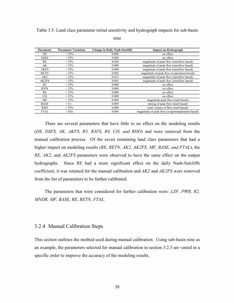
3.5 Land class parameter initial sensitivity and hydrograph impacts for
sub-basin nine …………….................................................................................38
3.6 River class parameter values obtained through manual calibration …………...42
3.7 Land class parameter values obtained through manual calibration ……………42
3.8 Pre-calibrated and manually calibrated Nash-Sutcliffe coefficients …………...43
3.9 Automated calibration parameters selected by hydrologic process …………....45
3.10 Sub-basins used for automated calibration …………………………………….47
3.11 River class parameter values obtained through automated calibration ………...49
3.12 Land class parameter values obtained through automated calibration ………...49
3.13 Nash-Sutcliffe coefficients from manual and automated calibrations …………50
3.14 Nash-Sutcliffe coefficients from pre-calibrated and automatically calibrated
model …………………………………………………………………………..51
4.1 Rain gauge removal order ……………………………………………………...57
4.2 Rain gauges removed for each de-clustering trial ……………………………..58
4.3 Initial daily Nash-Sutcliffe coefficients for de-clustering models ……………..60
4.4 Initial monthly Nash-Sutcliffe coefficients for de-clustering models ………….61
4.5 Initial and calibrated weighted daily Nash-Sutcliffe coefficients for
de-clustering trials ……………………………………………………………..64
4.6 Calibrated daily Nash-Sutcliffe coefficients for each de-clustering trial………64
4.7 Calibrated monthly Nash-Sutcliffe coefficients for each de-clustering trial …..65
viii
List of Figures
1.1 Satellite image of study area with gridded overlay of watershed boundaries ......4
2.1 Example study area for de-clustering method …………………………………17
2.2 Group response unit and runoff routing concept ………………………………18
3.1 Upper South Saskatchewan River basin ……………………………………….24
3.2 Gridded form of Upper South Saskatchewan River watershed used in
WATFLOOD …………………………………………………………………..24
3.3 River class assignment for Upper South Saskatchewan River used in
WATFLOOD …………………………………………………………………..25
3.4 Land usage for the Upper South Saskatchewan River watershed ……………..26
3.5 Sub-basins and stream gauge locations on the WATFLOOD model grid for the
Upper South Saskatchewan River ……………………………………………...27
3.6 Weather station locations in the Upper South Saskatchewan River watershed ..30
3.7 Sub-basins selected for manual calibration ……………………………………35
3.8 Measured streamflows vs. modeled streamflows from pre-calibrated model of
Red Deer River below Burnt Timber Creek (sub-basin 9) …………………….39
3.9 Measured streamflows vs. modeled streamflows from manual calibration of Red
Deer River below Burnt Timber Creek (sub-basin 9) …….................................41
3.10 Automated calibration parameter adjustment flow chart ……………………....46
3.11 Sub-basins used for automated calibration …………………………………….48
3.12 Measured streamflows vs. modeled streamflows from pre-calibrated model of
Red Deer River below Burnt Timber Creek (sub-basin 9) …………………….52
3.13 Measured streamflows vs. modeled streamflows from manually calibrated
model of Red Deer River below Burnt Timber Creek (sub-basin 9) …………..52
3.14 Measured streamflows vs. modeled streamflows from automated calibration of
Red Deer River below Burnt Timber Creek (sub-basin 9) …………………….53
4.1 Rain gauges used for de-clustering trials …………………………………........59
4.2 River class parameter variation resulting from de-clustering trials ……............62
4.3 Land class parameter variation resulting from de-clustering trials …………….63

ix
4.4 Daily Nash-Sutcliffe values from de-clustering trials …………………………66
4.5 Monthly Nash-Sutcliffe values from de-clustering trials ……………………...66
4.6 Sub-basin 16-25 shown with full precipitation set locations …………………..67
4.7 Sub-basin 26-29 shown with full precipitation set locations …………………..67
A.1 Grid cell numbers ………………………………………………………………80
A.2 Grid cell areas ………………………………………………………………….81
A.3 Flow direction for each grid cell ……………………………………………….82
A.4 Grid cell elevations …………………………………………………………….83
A.5 Grid cell contours ……………………………………………………………...84
A.6 Number of channels in each grid cell ………………………………………….85
A.7 Land class 1 (dense forest) allocation for each grid cell ……………………….86
A.8 Land class 2 (light forest) allocation for each grid cell ………………………..87
A.9 Land class 3 (mixed forest) allocation for each grid cell ………………………88
A.10 Land class 4 (open) allocation for each grid cell ………………………………89
A.11 Land class 5 (wetland) allocation for each grid cell …………………………...90
A.12 Land class 6 (agricultural) allocation for each grid cell ……………………….91
A.13 Land class 7 (glacier) allocation for each grid cell …………………………….92
A.14 Land class 8 (water) allocation for each grid cell ……………………………...93
A.15 Land class 9 (impervious) allocation for each grid cell ………………………..94

1
Chapter 1
Introduction
1.1 Problem Description
Hydrologic simulation models have been used since 1966 to help hydrologists better
understand different hydrologic processes, describe the hydrology of a specific region,
and to predict the potential hydrologic impact that future development may cause. While
hydrologic models are often useful, accurate model predictions can be difficult to
achieve. Hydrologic modeling software typically requires large quantities of input data
that may necessitate extensive pre-processing before a model can be properly run.
Additionally, the number of unknown parameters in hydrologic models is often large, and
a significant degree of calibration may be required to ensure the model is able to
represent historical and future trends.
For regional scale hydrologic models, data management and calibration can be a
very complex task. The modeled region of interest can contain diverse land types, which
can be difficult to classify and parameterize. Regional scale models can also have
inconsistent and poorly distributed input data (i.e., precipitation, temperature, wind speed,
and humidity). The availability and relative density of weather stations strongly
influences the accuracy estimated rainfall, temperature, etc., between stations. Since these
inputs drive the model, poor data density or interpolation can lead to flawed results.
This thesis presents two contributions to the scientific literature on regional-scale
hydrologic modeling. First, a general approach used for calibration of regional scale
hydrologic models, with application to a WATFLOOD model of the Red Deer River, the
Bow River, and the Old Man River watersheds in Alberta, is presented. In this method, a
structured approach towards manual calibration is initially used to determine parameters
that have a significant influence on model output. This parameter set is then subjected to
automated calibration to optimize parameter values. The objective function used for the
automated calibration is calculated based on the model results from multiple sub-basins.

2
The second component of this study is an investigation into the impacts of de-clustered
precipitation data upon hydrologic model calibration. The goal of this portion of the
study is to determine a relationship between gauge density and a hydrologic model’s
potential to be accurately calibrated.
1.2 Objectives
There are two objectives of this study. The first is to calibrate a regional scale hydrologic
model using both manual calibration and automatic calibration methods. The steps taken
to meet this objective include:
1. Model development and assessing project limitations: The study area and the
pre-calibrated model are assessed with the purpose of determining major study
limitations. Three types of limitations are encountered. The first is caused by
missing historic data. Data sets used to fuel the model (historic precipitation), and
data sets used to evaluate the model (historic streamflows) both have missing data
for portions of the study period. The second limitation is the unknown behavior
of certain man-made hydrologic features within the study area such as dams,
irrigation canals, and reservoirs, and incorporating these features into a
continuous model is outside the scope of this project. The final limitation comes
from WATFLOOD itself. While WATFLOOD is designed to handle many
hydrologic features, not all processes can be modeled and this puts restrictions on
the ability to accurately model portions of the watershed.
2. Manual calibration: This involves trial and error variation of each of the
unknown model parameters with the purpose of determining how each parameter
influences modeling results, and to improve the modeling results. Each parameter
is also given a range based on model sensitivity that is used during automated
calibration. Both subjective visual inspection and a formal objective function are
used for model comparison in this step.

3
3. Automated calibration: The objective function used in this step is designed to
consider the results of multiple sub-basins in the model. Using the parameter set
and ranges obtained through manual calibration, a search algorithm is used to
optimize the objective function and the find calibrated values for each parameter.
The calibration is performed based on the objective function alone and the model
is validated using the results from sub-basins not used in the objective function
calculation.
The second objective of this study is to assess the relationship between rain gauge
density and calibration accuracy. Four models are set up, each with a reduced rain gauge
density. Each model is calibrated using the calibration method used in the first portion of
the study, and impacts of the de-clustered input data sets are discussed and interpreted.
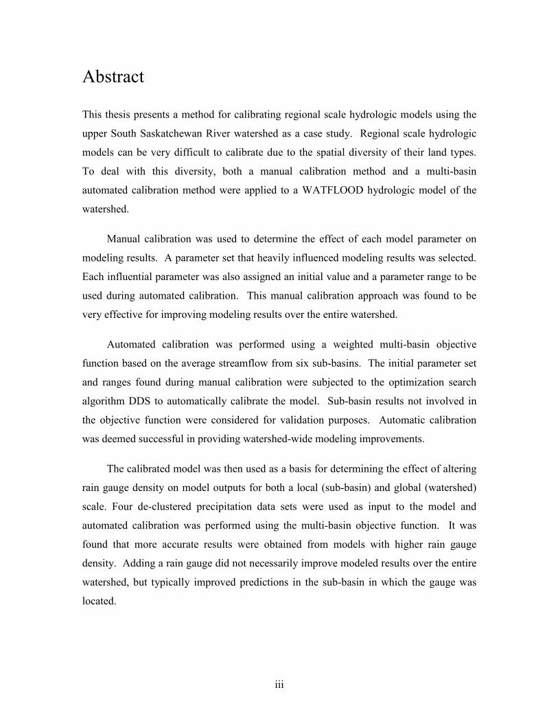
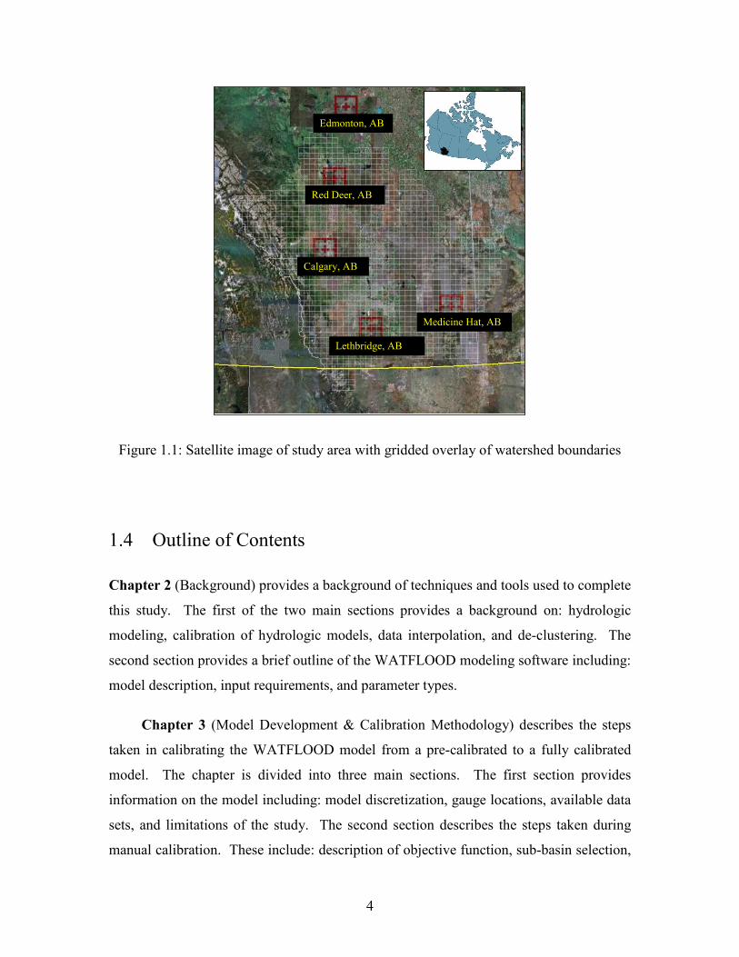
1.3 Site Description
Located mostly in southern Alberta, Canada, the watershed used for this study is the
upper South Saskatchewan River, which consists of the Red Deer River, the Bow River,
and the Old Man River. With a contributing area of over 120,000 km2, these three basins
flow through diverse land types including mountains, foothills, and prairies. The study
area drains from west to east between the Rocky Mountains at the western border of
Alberta (continental divide) and the prairies of western Saskatchewan. Figure 1.1 shows
a satellite image of the study area with an overlay of the boundaries of the watersheds.
4
Calgary, AB
Red Deer, AB
Edmonton, AB
Medicine Hat, AB
Lethbridge, AB
Figure 1.1: Satellite image of study area with gridded overlay of watershed boundaries
1.4 Outline of Contents
Chapter 2 (Background) provides a background of techniques and tools used to complete
this study. The first of the two main sections provides a background on: hydrologic
modeling, calibration of hydrologic models, data interpolation, and de-clustering. The
second section provides a brief outline of the WATFLOOD modeling software including:
model description, input requirements, and parameter types.
Chapter 3 (Model Development & Calibration Methodology) describes the steps
taken in calibrating the WATFLOOD model from a pre-calibrated to a fully calibrated
model. The chapter is divided into three main sections. The first section provides
information on the model including: model discretization, gauge locations, available data
sets, and limitations of the study. The second section describes the steps taken during
manual calibration. These include: description of objective function, sub-basin selection,

5
a description of calibrated parameters, parameter sensitivity, and calibration results. The
final section of this chapter outlines how the automated calibration process was
completed. This section includes: parameter selection, parameter ranges, basin selection
for the multiple basin automated trails, and calibration results.
Chapter 4 (Impacts of Precipitation De-clustering) contains information on the de-
clustering experiment. The first of the two main sections describes the method used for
de-clustering the rain gauge data and the interpolation used to create the new data sets.
The second section presents the automated calibration results for each de-clustering trial,
and an assessment of the impacts of data density upon model calibration and
performance.
Chapter 5 (Summary & Discussion) provides a summary of the results obtained in
this thesis and contains a brief discussion of the significance of this work, future
considerations, and recommendations.

6
Chapter 2
Background
This study uses a multiple basin calibration approach to calibrate a regional scale model
comprised of multiple sub-basins and multiple stream gauges. This multiple basin
calibration method has the benefit that it allows a hydrologic model to be efficiently
calibrated when testing the model against rain gauge density alterations and de-clustering.
This chapter is dedicated to providing a background on both the techniques and
tools used to complete this study. The literature review (section 2.1) provides a
background on hydrologic modeling, calibration of hydrologic models, and methods for
interpolating and de-clustering rain gauge data. This chapter also provides a brief
summary of the WATFLOOD hydrologic modeling software (section 2.2).
2.1 Literature Review
2.1.1 Hydrologic Modeling
Hydrologic modeling is an attempt to represent different aspects of the hydrologic cycle
through statistical and/or mathematical simulation. It is a powerful tool that can be used
for both research purposes and for planning and development (Seth, 2004). Software
codes capable of simulating several parts of the hydrologic cycle are sometimes used to
represent an entire hydrologic system. Although the understanding of the hydrologic
cycle continues to improve, there is still much to be learned on how hydrologic systems
function, and how they can be better modeled to meet the needs of today’s researchers
and practitioners.
Computer-based hydrologic modeling started during the 1960’s when large
computer models were used to attempt to match historical hydrologic data. The ability to
7
perform many calculations using the computer was helpful for answering complicated
hydrologic questions.
The first computational hydrologic model was created at Stanford University and
was called the Stanford Watershed Model (Crawford & Linsley, 1966). It was able to
effectively simulate precipitation, evaporation, evapotranspiration, infiltration, surface
runoff, ground water flow, and streamflow (Bedient & Huber, 2002). The goal of these
earlier programs was to continuously simulate hydrologic processes and to include all of
the interacting processes in the same model structure (Crawford & Burges, 2004).
Since the development of these early computer-based hydrologic models, there have
been several types of software of varying complexity developed to assist hydrologists in
understanding complex hydrologic processes. As a result of continued advancement,
hydrologic modeling remains a key component of the advancement of hydrologic study.
Often, the development and calibration of hydrologic models gives insight into the
limitations of modeling specific hydrologic processes and leads to improvements in
modeling software. Additionally, increased computing power has created a demand for
more field data, which in turn allows for further hydrologic study. If applied correctly,
hydrologic models are currently the best way to estimate and understand complex
hydrologic systems (Bedient & Huber, 2002). There are many types of hydrologic
models, but the three most used types are: conceptual, stochastic, and physically-based
models.
Conceptual hydrologic models use very little information about the watershed, and
provide efficient estimates of how a watershed will respond to precipitation (Fenicia et
al., 2007). Some examples of conceptual hydrologic models are linear models, Nash
instantaneous unit hydrograph, the rational method, and kinematic or dynamic wave
methods for overland flow (Bedient & Huber, 2002).
Stochastic hydrologic models use mathematics and statistics to produce an output
based on a set of input data. A typical example of this would be producing synthetic
streamflows based on a set of input precipitation data based on historical statistics from
the specific watershed (Bedient & Huber, 2002).
8
Physically-based hydrologic models attempt to simulate the hydrologic processes as
they occur in the real world and are based on our understanding of the physics of
individual hydrologic processes, e.g., infiltration, snowmelt, etc. (Seth, 2004).
Physically-based distributed models can be applied to many types of hydrologic problems
(Seth, 2004). Some common inputs for a physically based hydrologic model include
precipitation, temperature, wind speed, humidity, and initial snow depth. These are used
as input parameters to mass transfer and energy budget equations that can be used to
model snow melt, evaporation, and infiltration (Bedient & Huber, 2002).
Physically-based hydrologic models are typically set up to be single event models
or continuous models. Single event models are primarily used for the design of hydraulic
systems to handle large floods based on a single extreme precipitation event. They are
convenient in that it is easy to set up the antecedent conditions in the system, and because
they have very short run times. Continuous models are long term simulations that usually
simulate several historic precipitation events. These can range from a single season to
many years. Like single event models, continuous models can also be used in the design
of hydraulic systems, but may also include simulation goals related to base flow
depletion/recharge, evaporation, or snow melt as these hydrologic processes take much
longer than would be simulated by a single event model.
2.1.2 Calibration of Hydrologic Models
Most hydrologic models contain general equations that are intended to be useful over a
large variety of geographic areas. These equations include parameters that can be varied
to account for the hydrology of a specific study area. Without calibration, such “general-
purpose” models will not likely produce accurate, acceptable results (Debo & Reese,
2002). This is partly because the equations intended to represent natural hydrologic
processes contain parameters and coefficients that are difficult if not impossible to
estimate from field data. Once a hydrologic model has been set up to represent the
diversity of the specified, model calibration can begin.

9
Calibration of a hydrologic model is the process by which parameters that heavily
influence model output are modified in an attempt to replicate the model outputs with
historic data from the watershed (Debo & Reese, 2002). For example, it is often
desirable for the model to be able to simulate historic streamflow data given historic
precipitation data. Depending on the purpose of the model, the requirements for
calibration may vary: one model may be intended to best meet peak flows, another may
be focused on simulating low or mid flows. The goals of calibration are typically
expressed in terms of a calibration objective function defined such that the optimal
solution is that with the smallest (or largest) objective function.
There are several objective functions that can be used to assess the accuracy of a
hydrologic model. The objective function selected may depend on the specific goals of
the study. The most common objective function used for calibration of hydrologic
models is the Nash-Sutcliffe model efficiency coefficient (Nash & Sutcliffe, 1970)
defined as:
∑
∑
=
=
−
−
−= T
tO
tO
T
t
tm
tO
QQE
1
2
1
2
)(
)(1 (2.1)
where Qo is observed discharge and Qm is modeled discharge. The coefficient is a
measure of the model’s predictive ability. The Nash-Sutcliffe model efficiency
coefficient has a range of -∞ to 1.0. The maximum value of 1.0 indicates a perfect match
between the model and the observed data. A value of 0.0 indicates that the model is as
good of a predictor as the mean of the observed flows. A value greater than 0.0 means
that the model is a more accurate predictor than the mean of the observed data, while a
value less than 0.0 results when the model is a less accurate prediction than the mean of
the observed data.
While the Nash-Sutcliffe model efficiency coefficient is one of the most common
methods for evaluating the accuracy of a hydrograph, it has been shown that very poor
models can possess relatively high Nash-Sutcliffe coefficients, and low Nash-Sutcliffe

10
coefficients can result from a good model. Because of this, it is beneficial not to
conclude on the performance of a model based on the Nash-Sutcliffe coefficient alone
(Jain & Sudheer, 2008).
Once an objective function is selected, the calibration process can be executed using
either manual calibration or automated calibration. Manual calibration is a method in
which parameters are manually varied one at a time in an attempt to improve the model
results and gain an understanding of how certain parameters influence model outputs.
Automated calibration is a method where parameters are simultaneously varied using a
search algorithm to find the parameter set that produces the most accurate model results.
Manual calibration is the most widely used method to calibrate hydrologic models
(Boyle et al., 2000). Usually used in the early stages of the calibration of a hydrologic
model (prior to automated calibration), it is a method that essentially uses trial-and-error
parameter adjustment to improve the model and determine a good parameter set (Madsen,
2000).
Often, the comparison between the observed hydrograph and the simulated
hydrograph is made purely from visual inspection. Experienced modelers can obtain
very accurate models through manual calibration, but without an objective function, it is
difficult to quantify its quality in comparison to equally plausible models (Madsen,
2000). If automated calibration is to take place following manual calibration, it can be a
good idea to monitor the selected objective function during manual calibration so that a
better understanding can be gained of how that objective function is reacting to visual
improvements in the model.
Manual calibration provides modelers with some advantages over automated
calibration. Because parameters are varied one at a time, modelers see each varied
parameter changes model outputs. This allows a modeler to determine the set of
dominant parameters that strongly influence the specific watershed. Through this
process, a modeler is also able to understand the sensitivity of each parameter and
determine reasonable starting points and ranges for the parameter set to be used during
automated calibration; this will reduce the number of iterations required during

11
automated calibration. Modelers that manually calibrate their models gain a better
understanding about how different hydrologic processes impact the output hydrographs.
Additionally, these modelers are better prepared to identify problems that may be
encountered during automated calibration (Madsen, 2000).
Though popular and useful, manual calibration has drawbacks. Each model run
requires visual hydrograph analysis (and possibly objective function calculation) and
parameter adjustment by the modeler, and makes manual calibration a labor intensive
process. The method can be complicated, and expertise from one modeler is difficult to
pass on to another modeler as the best method for improving one’s manual calibration
skill is through hands on experience and training (Boyle et al., 2000).
An increasingly popular method of improving the quality of hydrologic models is
automated calibration; however, because automated calibration approaches often require
a mathematical background and use more complicated computational tools than manual
calibration, it still remains unused by many modelers (Boyle et al., 2000). Each
parameter varied in automated calibration must be given a range defined by maximum
and minimum values. The set of specified parameter ranges is called the parameter
space. Automated calibration uses optimization algorithms to search the parameter space
to find the parameter set that will result in the best value of the objective function. The
technique is not labor intensive, nor is it biased by the modeler’s expert knowledge or
opinions (Madsen, 2003), except in the selection of the objective function and parameter
ranges.
Three things are necessary to complete an automated calibration: an objective
function, a parameter set with an initial parameter space, and an optimization algorithm.
As previously discussed, there are different objective functions to choose from. Properly
selecting an objective function that meets the needs of the specific study is critical for
developing a model that meets the needs of the modeler. It has been found that
performing a single criteria approach to automated calibration can lead to good curve
fitting, but can lead to a parameter set that is hydrologically unrealistic (Boyle et al.,
2000). A method that can help to avoid this situation is to complete in-depth manual

12
calibration prior to automated calibration to see that there are hydrologically realistic
parameter values.
The final component of an automated calibration is an optimization algorithm. For
this, there are many to choose from, which can be categorized as either local or global
search methods. Both local and global search methods are used for computationally
complex problems in which no specific algorithm can be used to solve the problem in its
entirety (MacFarlane & Tuson, 2008). While both methods may start searching from the
same point in the parameter space, local search methods will improve the result of the
objective function towards a local maximum (or local minimum) value. Global search
methods are designed to solve optimization problems that may have multiple optima
(Zabinsky, 1998).
Because rainfall runoff models can have numerous locally optimal solutions within
the parameter space (Duan et al., 1993), local search methods will often not produce a
global optimum because the results will depends on the search starting point. Because of
this, global search methods should be employed to solve hydrologic calibration problems
(Madsen, 2000). Some of the most popular methods for automated calibration are
evolution-based searches such as the shuffled complex evolution (Duan et al., 1993) and
genetic algorithms (Wang, 1991). Several studies (Duan et al., 1993; Gan & Biftu, 1996;
Cooper et al., 1997; Kuczera et al., 1997; Franchini et al., 1998; Thyer et al., 1999) have
compared genetic algorithms and shuffled complex evolution (SCE), and find that the
SCE algorithm is more effective and efficient. It has been widely used in conceptual
rainfall runoff models (Madsen, 2000).
The optimization algorithm chosen for this study is a dynamically dimensioned
search (DDS) (Tolson & Shoemaker, 2007). The DDS algorithm is novel and simple
stochastic single-solution based heuristic global search algorithm (Tolson & Shoemaker,
2007). With a purpose of finding good global solutions instead of globally optimal
solutions, the algorithm is designed to scale the search to the user-specified number of
function evaluations (Tolson & Shoemaker, 2007). Initially, the algorithm searches
globally, and as the number of specified objective function evaluations approaches, the

13
search becomes more localized (Tolson & Shoemaker, 2007). To interact with a
hydrologic model DDS requires a parameter set with pre-determined user-assigned
ranges for each parameter.
DDS has been compared to the SCE method, and has been shown to require only
15-20% of the model evaluations used by the SCE method to obtain equally good values
of the objective function (Tolson & Shoemaker, 2007).
2.1.3 Temporal and Spatial Data Interpolation Methods
The most important input to a hydrologic model is the temporal and spatial distribution of
rainfall (Lynch & Schulze, 1995; Yoo, 2002). The output of a regional scale model with
sparse rainfall data can be strongly influenced by the interpolation routine that generates
rainfall values for unmeasured areas of the watershed, and having an accurate areal
precipitation representation is crucial in hydrologic modeling (Dorninger et al., 2008).
Selecting a method to estimate rainfall distribution from rain gauges can often be a time
consuming but important problem (Lynch & Schulze, 1995).
In regional scale models with complex terrain, properly using the available data is
an important aspect of developing an accurate model (Dorninger et al., 2008). Rainfall
interpolations for regional scale models are effected by the distribution and density of
rain-gauges as this can significantly contribute to the sampling error in the estimation of
the total volume of rainfall over a given area (Yoo, 2002). Beven and Hornberger (1982)
found that, for predicting streamflow hydrographs, the correct assessment of rainfall
input volume is more important that the spatial rainfall pattern.
While a majority of this study is dedicated to the calibration of a regional scale
model, once complete, the calibration method is tested using several rain-gauge input
data sets. Input data sets are generated by interpolating precipitation input sets that
decrease in density with each subsequent trial. Though the method of interpolation is not

14
varied to generate these data sets, it is a key aspect of this study and as such must be
selected carefully.
Many techniques exist that modelers use to estimate rainfall between rain gauge
point measurements. Common techniques include: inverse distance interpolation,
Shepard’s weighted interpolation, Schafer interpolation, SACLANT interpolation, and
Kriging (Lynch & Schulze, 1995).
Inverse distance weighting (IDW) is determined according to the following
equations (Shepard, 1968):
∑=
=n
iii fwyxF
1
),( (2.2)
∑=
−
−
=n
jj
ii
d
dw
1
2
2
(2.3)
where d is the distance between the location (x,y) where rainfall is unknown and the
given weather station (i), and F is the value of rainfall at the given weather station.
Shepard’s method employs the same weighting function, but only within a certain radius;
otherwise the weighting function is equal to zero. The radius should be selected based on
the geographic density of the data points (gauge density), and should be chosen so that
each sample radius includes at least five sample points (Yoeli, 1975).
Schafer interpolation makes use of the assumption that daily rainfall distribution
similarly resembles median monthly rainfall distribution (Lynch & Schulze, 1995). The
daily rainfall measurements from each rain gauge station are transformed into a
percentage of the median monthly rainfall at that station for that specific data (Schafer,
1991). Those values are interpolated using a two dimensional interpolation technique
onto a rectangular grid (SACLANT, 1979). The interpolated values are then multiplied
by the gridded median monthly rainfall values to result in daily rainfall estimates (Dent,
Lynch and Schulze, 1988).
15
SACLANT interpolation is another two dimensional interpolation used for a
rectangular-gridded shaped study area, such as that used in the WATFLOOD software.
Values are initially assigned to each unknown point in the rectangular grid and then an
iterative process is performed where the unknown values are altered (improved) until the
surface of the precipitation values has obtained a targeted value of smoothness through
the known data points (SACLANT, 1979).
The Kriging method of interpolation uses a semi-variogram model to interpolate a
set of points (ArcInfo, 1991). The semi-variogram is a function that represents the
expected difference in value between sample points based on a given radius and
orientation (Clark, 1979). This model can be altered to be spherical, circular,
exponential, Gaussian, linear, universal linear or universal quadratic. A study
investigating the influence of different semi-variogram models (Lynch & Schulze, 1995)
found the universal linear model to produce the lowest root mean square errors when
attempting to interpolate known rainfall data. Statistical methods like Kriging can be
optimal in a statistical sense but are not applicable to some studies (Ahrens, 2005).
It has been found that for a regional scale models with a strong climactic gradient
and a sparse data set that IDW and Kriging are the most efficient towards generating a
model that can produce accurate hydrographs when calibrated (Ruelland et al., 2008).
The IDW method was found to be a significantly less time consuming process relative to
Schafer, SACLANT, and Kriging (Lynch & Schulze, 1995), and is the method selected
for this study.
2.1.4 De-Clustering
While it has been found that varied rain-gauge density can have very little effect on
modeling results in regions with relatively high rain-gauge densities (Allen &
DeGaetano, 2005), this study focuses on a region with a sparse, poorly distributed data
set. For this study, rain-gauge density will be decreased using the de-clustering method

16
described in this section, and the impacts on hydrologic model calibration will be
assessed.
De-clustering is a term used to describe a method in which data points are removed
to reduce the known, unknown, or estimated negative effects of clustered data to obtain a
data set that is more representative of underlying data (Smith, Goodchild, Longley,
2006). While several methods for de-clustering data exist, the technique has not been
extensively studied in the context of hydrologic modeling. Ahrens (Ahrens, 2005) found
a slight improvement using de-clustering for one of four rain gauge densities evaluated.
The method used by Ahrens (Ahrens, 2005) selected the closest pair of rain gauges and
eliminated the gauge which had the next closest rain gauge to it. For this study, de-
clustering will be performed using a search that will calculate a “clustering index” for
each rain gauge as follows:
∑=
=N
iidCI
1
2 (2.4)
where di is the distance between the selected rain gauge and the closest neighboring rain
gauge and N is the number of neighboring rain gauges used to calculate CI. For each rain
gauge, di is calculated for the closest four neighboring rain gauges and the gauge with
lowest CI is removed and the process is repeated. An example study area is shown below
in figure 2.1. In this example, the x-y locations of the rain gauges, labeled Xi, are shown
in table 2.1.
Table 2.1 – De-clustering example station locations
X Coordinate Y CoordinateX1 0 0X2 2 0X3 4 0X4 1 1X5 3 1X6 4 2X7 1 3

17
X1 X2 X3
X4 X5
X6
X7
0 2 4
0
1
2
3
Figure 2.1 – Example study area for de-clustering method
The corresponding CI values are calculated (equation 2.4) for each rain gauge and
the results are displayed in table 2.2.
Table 2.2 – Example CI calculation
X1 X2 X3 X4 X5 X6 X7 Min 1 Min 2 Min 3 Min 4 Sum (CI)X1 - 16 256 4 100 400 100 4 16 100 100 220
X2 16 - 16 4 4 64 100 4 4 16 16 40
X3 256 16 - 100 4 16 324 4 16 16 100 136
X4 4 4 100 - 16 100 16 4 4 16 16 40X5 100 4 4 16 - 4 64 4 4 4 16 28
X6 400 64 16 100 4 - 100 4 16 64 100 184X7 100 100 324 16 64 100 - 16 64 100 100 280
Table 2.2 shows the CI calculated using the lowest four distance squared values for
each rain gauge. The gauge selected through this method was gauge X5 with a CI of 28.
That gauge would be removed from the interpolation, and if further de-clustering was
desired, the process would be repeated, but starting with the updated gauge distribution.

18
2.2 Watflood
The hydrologic model used for the study is WATFLOOD. It is a physically-based
routing model combined with a conceptual hydrologic simulation model (Kouwen, 2007).
In WATFLOOD, a watershed is divided into a Cartesian grid, and each grid square is
subdivided into one or more land use types based on satellite imagery. The behavior of
each assigned land class is then governed by the equations of conceptual hydrologic
models and the land class parameters of WATFLOOD (section 2.2.2). An example of
how a specific grid square is handled is shown in figure 2.2.
Figure 2.2 – Group response unit and runoff routing concept (Donald, 1992; Kouwen,
2007)
In figure 2.2, the grid square is allocated in to land types (A, B, C, D) based on the
satellite image, and each land type is handled in the model as a separate watershed. The
runoff from each of the individual land class models is added to the physically based
streamflow routing model (Kouwen, 2007).

19
WATFLOOD simulates only a subset of the physical processes occurring in nature,
but includes: infiltration, evaporation, snow accumulation, interflow, base flow, and
overland channel routing (Kouwen, 2007).
2.2.1 Model Requirements
The WATFLOOD model used for this calibration is essentially fuelled by just two
hydroclimatic inputs: temperature and rainfall. Each of these inputs is taken from historic
data sets, and unknown data points (grid cells) are interpolated. Additionally, each grid
cell requires information to describe the specific land it represents including (Kouwen,
2007):
N – Grid cell number
NEXTI – Receiving cell number. This tells WATFLOOD which grid cell the streamflow will be sent to.
XX, YY – Grid cell location from bottom left corner of grid.
DA– Drainage area in km2.
IBN – River class
1,2,…N – Fractions in each land cover type.
The model requires parameter assignment for both the land type and river class
parameters (described in section 2.2.2) as well as values for the initial conditions of both
snow depth and streamflow, all of which can be modified in the WATFLOOD input files.
2.2.2 Model Parameters
While directly measured meteorological data is used to fuel the model, model behavior
heavily relies on the values of many adjustable system parameters. The primary
parameters driving the model results may be divided into land class parameters, which
20
are dictated by land use and soil type, and river class parameters, which are dictated by
drainage area, geographic location, and sub-basin boundaries. The default values listed
with each parameter shown are not considered WATFLOOD specific defaults, but are
simply the defaults arrived at in this study.
There are five river class parameters. The first two are related to how
WATFLOOD handles base flow:
LZF – Lower zone function (default = 0.200 x 10⁻⁵)
PWR – Exponent on lower zone function (default = 0.200 x 101)
Both LZF and PWR effect base flow the depletion function (QLZ) according to the
following equation:
PWRLZSLZFQLZ *= (2.5)
where LZS is the lower zone storage in each grid cell and QLZ is the lower zone flow
(base flow). All land classes present in each grid (except impervious) contribute to the
lower zone storage.
There are two river roughness parameters:
R1 – Flood plain roughness coefficient (default = 0.200 x 101)
R2 – River channel roughness coefficient (default = 0.100 x 101)
Both R1 and R2 are transformed to values of Manning’s n and then subject to
Manning’s equation to determine the average channel velocity:
21
32
SRnk
V h= (2.6)
where k is a conversional constant, n is the Gaucklet-Manning coefficient, Rh is the
hydraulic radius, and S is the slope of the water surface.
21
MNDR – Meander factor (default = 0.100 x 101)
The meander factor is a ratio of how long each channel in the grid is relative to the
length of the grid.
The parameters related to land use are as follows:
• DS – Depression storage (mm) (default = 0.200 x 10²)
• DSFS – Depression storage for snow (mm) (default = 0.200 x 10²)
• RE – Interflow depletion coefficient (default = 0.302 x 10)
• AK – Soil permeability for bare ground (default = 0.904 x 101)
• AKFS – Soil permeability under snow (default = 0.140 x 10²)
• RETN – Upper zone specific retention (default = 0.750 x 10²)
• AK2 – Upper zone resistance factor for bare ground (default = 0.125 x 10)
• AK2FS – Upper zone resistance factor under snow (default = 0.984 x 10)
• R3 – Overland roughness for bare ground (default = 0.101 x 10²)
• R3FS – Overland roughness under snow (default = 0.394 x 10²)
• R4 – Impervious area roughness (default = 0.100 x 10²)
• CH – Channel efficiency factor (default = 0.900 x 10)
• MF – Melt factor (mm/°C/hr) (default = 0.139 x 10)
• BASE – Base melt temperature (°C) (default = -0.115 x 101)
• RHO – Snow density (relative to rho H20) (default = 0.333 x 10)
• FTAL – Forest vegetation coefficient (default = 0.850 x 10)
Not all parameters described above will have a significant effect on modeling
results. Depending on the specific model, certain parameters can strongly influence
different portions of the model. The entire parameter set will be analyzed for
significance during manual calibration; however, not all parameters will be adjusted
during automated calibration.

22
Chapter 3
Model Development & Calibration
Properly calibrating a hydrologic model is an essential step towards using that model as a
basis for experimentation and understanding. While many methods of calibration can be
used to improve the accuracy a model’s outputs, no method can guarantee the most
accurate model possible; in fact, it is likely that no ‘best’ solution exists and that several
equally accurate models can be produced with very different parameter sets (Beven,
2000).
Parameters that affect the behavior of the entire model are sometimes determined
through the calibration of only one sub-basin. For local scale models, this can be very
effective since many parameters are not likely to vary significantly through the basin.
However, due to variation of land types of a regional scale model, calibrating parameters
one sub-basin at a time is less likely to produce a parameter set that represents the
behavior of the entire watershed; therefore, multi-basin calibration approaches are
needed. The calibration method described this chapter is performed on a regional scale
model. It promotes parameter determination through an objective function that is
calculated from the results in multiple sub-basins.
The following sections review the development of the hydrologic model for the
Upper South Saskatchewan River case study, as well as model calibration as it applies to
WATFLOOD hydrologic models. Section 3.1 outlines the model development and data
analysis that was performed prior to calibration. This includes the model discretization,
gauge locations, available data sets, and study limitations. Section 3.2 provides a
description of the manual calibration process. This section includes a description of the
objective functions used, sub-basin selection methods, a description of the parameters
used for calibration and how they affect model outputs, an example manual calibration
for a single sub-basin, and a summary of the calibration results. Section 3.3 outlines the
steps taken during automated calibration. These include a brief overview of the

23
optimization algorithm, a summary of the parameters selected and their optimization
ranges, a description of the objective function weighting method, an overview of the sub-
basins used for the automated process, and a summary of the automated calibration
results.
3.1 Upper South Saskatchewan River Model Development
Before model calibration can begin, the study area and the available historic data must be
understood. This section provides an overview how the study area has been represented
using a WATFLOOD hydrologic model, a summary of the data sets available for the
study, and a review of some limitations that were encountered during model
development.
3.1.1 Study Area & Model Discretization
The watershed used for this study is the Upper South Saskatchewan River. Located in
southern Alberta, Canada, this watershed is made up of three major rivers: the Red Deer
River, the Bow River, and the Old Man River. The watershed has a contributing area of
over 120,000 km2 and flows east from the continental divide. For the purpose of
developing a regional scale hydrologic model of the watershed, the study area has been
divided up into 1341 grid cells, each with an area of approximately 100 km2 (10 km x 10
km). Figure 3.1 shows a map of the study area, while Figure 3.2 shows the gridded form
of the study area.

24
Figure 3.1: Upper South Saskatchewan River Basin (Alberta Environment, 2009)
Figure 3.2: Gridded form of Upper South Saskatchewan River watershed used in
WATFLOOD

25
Each grid cell must have a designated river class, and must be assigned one or more
land uses. Using a combination of satellite imagery, sub-basin boundaries, and
contributing area, three river classes were designated. The three river classes are:
Class 1 – Mountain/Foothills stream (contributing area < 1000 km2 and visually
identifiable as a region with high vegetation from satellite imagery)
Class 2 – Prairie stream (contributing area < 1000 km2 and visually identifiable
as a region with low vegetation from satellite imagery)
Class 3 – Major River (contributing area > 1000 km2)
Figure 3.3 shows the assigned river classes for each grid cell.
Figure 3.3: River class assignment for Upper South Saskatchewan River used in
WATFLOOD
CLASS
1
2
3

26
For this study, land use was divided into nine land classes: dense forests, light
forests, mixed forests, open, wetlands, agriculture, glacier, water, and impervious. Each
land class was assigned using remotely sensed land cover data (Kouwen, 2007). Figure
3.4 shows the distribution of each land class in the watershed.
59.3%
27.0%
4.6%
3.4%
2.3%
1.5%
1.1%
0.3%
0.5%
0.0%
10.0%
20.0%
30.0%
40.0%
50.0%
60.0%
70.0%
Agricultural
Open
Mixed Forest
Dense Forest
Light Forest
Wetland
Water
Glacier
Impervious
Figure 3.4: Land usage for the Upper South Saskatchewan River watershed
As shown, a majority of the land use (86%) in the watershed is characterized as
agricultural or open land.
The model is set up to output streamflows at 30 grid cell outflow points in the
model which roughly corresponds to the 30 sub-basin stream gauges that exist in the
watershed and are shown on figure 3.5. The modeled (and measured) drainage areas and
land use for each sub-basin is shown in table 3.1.
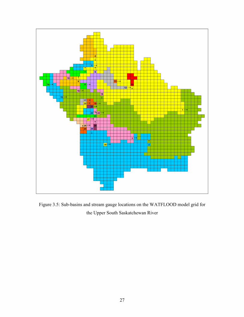
27
4
5
7 6
109 11
14 8 1312
1618
151720 19
211
22 2423
27
26 2825 29
3
30 2
Figure 3.5: Sub-basins and stream gauge locations on the WATFLOOD model grid for
the Upper South Saskatchewan River

28
Table 3.1: Land use for sub-basins in the Upper South Saskatchewan River watershed
Sub-basin Area Dense Forest Light Forest Mixed Forest Open Wetland Agricultural Glacier Water Impervious# (sq km) % % % % % % % % %1 46250 2.6 1.6 3.3 28.6 0.8 61.8 0.2 1.2 0.02 32089 4.4 2.9 7.8 12.4 1.9 69.3 0.0 1.1 0.03 6827 2.7 2.1 6.1 7.3 2.4 78.6 0.0 0.8 0.14 1966 0.0 0.4 13.3 13.2 0.5 72.6 0.0 0.0 0.05 784 10.9 3.7 17.0 18.2 0.4 50.0 0.0 0.0 0.06 2612 0.2 4.3 16.2 10.5 5.2 63.7 0.0 0.0 0.07 760 28.4 21.9 33.9 8.2 1.1 6.1 0.0 0.0 0.08 506 0.3 11.1 51.1 18.0 17.7 2.2 0.0 0.0 0.09 2418 36.8 15.1 1.4 34.9 7.3 0.0 3.0 1.5 0.010 1012 21.4 13.6 0.1 44.5 10.3 0.0 7.0 3.0 0.011 68 0.0 0.0 0.0 0.0 0.0 100.0 0.0 0.0 0.012 2398 0.0 0.0 0.0 0.8 0.0 99.2 0.0 0.0 0.013 25189 5.1 3.1 6.6 14.9 1.5 67.4 0.3 1.1 0.114 413 18.6 8.3 0.0 45.4 7.9 0.0 15.8 3.9 0.015 3494 21.8 12.2 1.0 46.9 8.5 0.0 5.7 3.9 0.016 321 22.4 14.4 50.3 10.8 1.2 0.0 0.2 0.9 0.017 351 7.8 8.0 33.8 19.4 11.4 19.2 0.0 0.0 0.018 310 0.0 0.0 0.0 0.0 0.0 100.0 0.0 0.0 0.019 1528 8.4 15.1 22.3 25.8 4.6 21.7 0.2 0.1 1.620 777 13.1 26.1 21.6 35.4 3.1 0.0 0.4 0.1 0.021 240 0.0 1.4 54.4 19.6 5.7 18.9 0.0 0.0 0.022 537 6.2 6.9 47.4 17.6 1.3 20.6 0.0 0.0 0.023 630 13.1 7.8 31.3 19.7 2.4 23.5 1.1 1.3 0.024 1513 7.7 5.7 29.8 15.5 1.5 38.9 0.4 0.5 0.025 233 62.9 15.3 5.1 13.9 2.6 0.0 0.0 0.3 0.026 771 22.0 13.8 26.2 21.1 17.0 0.0 0.0 0.2 0.027 129 0.0 3.0 79.0 11.0 2.0 5.0 0.0 0.0 0.028 226 0.0 0.0 0.5 14.4 0.0 85.6 0.0 0.0 0.029 64 0.0 0.0 61.0 29.0 5.0 5.0 0.0 0.0 0.030 91 0.0 0.0 0.0 1.0 0.0 99.0 0.0 0.0 0.0
3.1.2 Gauge Locations & Available Data Sets
For this study, the hydrologic model has been set up to simulate continuously from
January 1, 2002 to December 31, 2005. This study utilized historic data from 30 stream
gauges (Environment Canada, 2007a) and 28 weather stations (Environment Canada,
2007b). Stream gauge data are in the form of average daily flow from each stream. Each
stream gauge provides data for the corresponding sub-basin and is located at the outlet of
a grid cell.
The available historic streamflow data from each stream gauge determine which
sub-basins should be used for calibration. The available stream gauge data are shown in
table 3.2.

29
Table 3.2: Available historic streamflow data for the Upper South Saskatchewan River
watershed
2002 2003 2004 20051 - 05CK004 RED DEER RIVER NEAR BINDLOSS2 - 05AG006 OLDMAN RIVER NEAR THE MOUTH3 - 05AC023 LITTLE BOW RIVER NEAR THE MOUTH May 1 - Oct 31 May 1 - Oct 31 May 1 - Oct 31 May 1 - Oct 314 - 05CC007 MEDICINE RIVER NEAR ECKVILLE5 - 05CB004 RAVEN RIVER NEAR RAVEN6 - 05CB001 LITTLE RED DEER RIVER NEAR THE MOUTH7 - 05CA002 JAMES RIVER NEAR SUNDRE Mar 1 - Oct 31 Mar 1 - Oct 31 Mar 1 - Oct 31 Mar 1 - Oct 318 - 05CA012 FALLENTIMBER CREEK NEAR SUNDRE May 1 - Oct 31 May 1 - Oct 31 May 1 - Oct 31 May 1 - Oct 319 - 05CA009 RED DEER RIVER BELOW BURNT TIMBER CREEK10 - 05CA004 RED DEER RIVER ABOVE PANTHER RIVER Apr 1 - Oct 31 Apr 1 - Oct 31 Apr 1 - Oct 31 Apr 1 - Oct 3111 - 05CE011 RENWICK CREEK NEAR THREE HILLS12 - 05CE002 KNEEHILLS CREEK NEAR DRUMHELLER Apr 11 - Oct 31 Mar 13 - Oct 31 Mar 10 - Oct 31 Mar 1 - Oct 3113 - 05CE020 MICHICHI CREEK AT DRUMHELLER Mar 23 - Oct 31 Mar 13 - Oct 31 NO DATA Mar 1 - Oct 3114 - 05BA001 BOW RIVER AT LAKE LOUISE May 1 - Oct 31 May 1 - Oct 31 May 1 - Oct 31 May 1 - Oct 3115 - 05BB001 BOW RIVER AT BANFF16 - 05BG006 WAIPAROUS CREEK NEAR THE MOUTH17 - 05BH009 JUMPINGPOUND CREEK NEAR THE MOUTH18 - 05BH014 NOSE CREEK ABOVE AIRDIRE NO DATA NO DATA NO DATA May 1 - Oct 3119 - 05BJ010 ELBOW RIVER AT SARCEE BRIDGE Apr 16 - Oct 31 Apr 1 - Oct 31 Apr 14 - Oct 26 NO DATA20 - 05BJ004 ELBOW RIVER AT BRAGG CREEK21 - 05BK001 FISH CREEK NEAR PRIDDIS Mar 1 - Oct 31 Mar 1 - Oct 31 Mar 1 - Oct 31 Mar 1 - Oct 3122 - 05BL013 THREEPOINT CREEK NEAR MILLARVILLE Mar 1 - Oct 31 Mar 1 - Oct 31 Mar 1 - Oct 31 Mar 1 - Oct 3123 - 05BL014 SHEEP RIVER AT BLACK DIAMOND24 - 05BL012 SHEEP RIVER AT OKOTOKS25 - 05BL022 CATARACT CREEK NEAR FORESTRY ROAD26 - 05BL019 HIGHWOOD RIVER AT DIEBEL'S RANCH Mar 1 - Oct 31 Mar 1 - Oct 31 Mar 1 - Oct 31 Mar 1 - Oct 3127 - 05BL027 TRAP CREEK NEAR LONGVIEW May 1 - Oct 31 May 1 - Oct 31 May 1 - Oct 31 May 1 - Oct 3128 - 05BL023 PEKISKO CREEK NEAR LONGVIEW Mar 1 - Oct 31 Mar 1 - Oct 31 Mar 1 - Oct 31 Mar 1 - Oct 3129 - 05AB040 WILLOW CREEK AT SECONDARY 532 Mar 1 - Oct 31 Mar 1 - Oct 31 Mar 1 - Oct 31 Mar 1 - Oct 3130 - 05AB029 MEADOW CREEK NEAR THE MOUTH Apr 1 - Oct 31 Mar 1 - Oct 31 Mar 1 - Oct 31 Mar 1 - Oct 31
* * * * * * * * * * COMPLETE * * * * * * * * * *
* * * * * * * * * * COMPLETE * * * * * * * * * *
* * * * * * * * * * COMPLETE * * * * * * * * * *
* * * * * * * * * * COMPLETE * * * * * * * * * ** * * * * * * * * * NO DATA * * * * * * * * * *
* * * * * * * * * * COMPLETE * * * * * * * * * *
* * * * * * * * * * COMPLETE * * * * * * * * * *
* * * * * * * * * * COMPLETE * * * * * * * * * ** * * * * * * * * * COMPLETE * * * * * * * * * *
* * * * * * * * * * COMPLETE * * * * * * * * * *
* * * * * * * * * * COMPLETE * * * * * * * * * ** * * * * * * * * * COMPLETE * * * * * * * * * ** * * * * * * * * * COMPLETE * * * * * * * * * *
STATION # STATION NAMEDATA DAYS
* * * * * * * * * * COMPLETE * * * * * * * * * *
Weather stations provide temperature and precipitation data on a daily time scale.
The locations of each station are displayed in figure 3.6.

30
3 54
2
18
21
711
9
10 2028 6
8
26 1912
13 141 2717 22
25
24
16
1523
Figure 3.6: Weather station locations in the Upper South Saskatchewan River watershed
3.2 Manual Calibration
This section provides an outline of how manual calibration was performed on a
WATFLOOD model of the Upper South Saskatchewan River watershed. The purpose of
manual calibration is to determine a finite set of parameters that strongly influences
modeling outputs. These parameters will be manually adjusted to values that result in
significant improvements in model outputs. Selecting the influential parameter set and
31
determining an initial value for each parameter through manual adjustment reduces the
parameter set and parameter space to be used for automated calibration and may produce
more accurate results. Described here are the objective functions used during manual
calibration, the method used for selecting sub-basins to calibrate, a description of the
most relevant and sensitive parameters that control model outputs, sensitivity of
calibrated parameters, and results obtained from manual calibration.
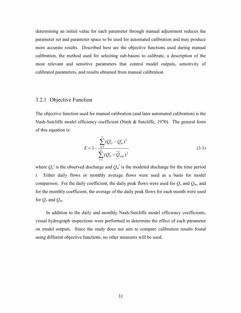
3.2.1 Objective Function
The objective function used for manual calibration (and later automated calibration) is the
Nash-Sutcliffe model efficiency coefficient (Nash & Sutcliffe, 1970). The general form
of this equation is:
∑
∑
=
=
−
−
−=T
tOm
tO
T
t
tm
tO
QQE
1
2
1
2
)(
)(1 (3.1)
where Qot is the observed discharge and Qm
t is the modeled discharge for the time period
t. Either daily flows or monthly average flows were used as a basis for model
comparison. For the daily coefficient, the daily peak flows were used for Qo and Qm, and
for the monthly coefficient, the average of the daily peak flows for each month were used
for Qo and Qm.
In addition to the daily and monthly Nash-Sutcliffe model efficiency coefficients,
visual hydrograph inspections were performed to determine the effect of each parameter
on model outputs. Since the study does not aim to compare calibration results found
using different objective functions, no other measures will be used.

32
3.2.2 Sub-basins Selected for Calibration
Each time a parameter was varied, the objective function was calculated for certain sub-
basins and visual inspection of the hydrographs was performed. Prior to any parameter
variation, the most appropriate sub-basins were selected for the purpose of learning the
most from each parameter variation.
Throughout the calibration process, results from certain sub-basins are used to
calibrate the model, while others are used for model validation. Validating the model is a
process in which results from some sub-basins that were not used to measure model
performance are compared to confirm model improvements. Limitations encountered in
this study restricted the number of sub-basins that could be trusted for calibration or
validation. Before sub-basin selection could take place, it was important to recognize and
address the limitations this case study. Here, these limitations can be classified into three
categories: data limitations, limitations caused by man-made hydraulic features,
hydrologic modeling limitations.
Data Limitations
While the streamflow data set contains historic measurements from 30 stream
gauges, it is clear from table 3.2 that the data set is not complete. Of the 30 stream gauge
locations, only 13 contain daily data for the entire study period. One gauge has no data
available for the study period, and several others are missing entire years of
measurements. The remaining gauges have only summer data, which can still be useful
for model validation purposes. The limited data set must be considered when selecting
basins for calibration (section 3.2.2).
Man-made Hydraulic Features
One portion of the study area is heavily affected by man-made reservoirs and
irrigation canals. Sub-basin three (see figure 3.5) is the watershed of the Little Bow
River and has a drainage area of approximately 6,800 km2. Of that area, drainage from
the upper 4,230 km2 is diverted into Travers Reservoir, and only 30 % of the annual
33
drainage is released back into the Little Bow River (Atlas of Alberta Lakes, 2005). The
other 70% of the drainage is diverted into Little Bow River Lake which feeds irrigation
canals for the region. Since the drainage released to the Little Bow River is controlled
and depleted rather than naturally drained, the model output from this sub-basin, which
only considers environmental influences, can not be used for calibration. Since this sub-
basin makes up over 20% of the drainage area for Oldman River watershed (sub-basin 2),
modeling results from the Oldman River are not useful for calibration.
Hydrologic Modeling Limitations
Hydrologic modeling limitations are the modeling software’s inability to represent
certain hydrologic processes. Here, the major hydrologic modeling limitation is the
simplification of processes simulated on prairie agricultural land use. Fifty-nine percent
of the entire watershed is allocated as agricultural use, most of which is located in the
prairie region of the study area. Two aspects of prairie hydrology make hydrologic
modeling on a regional scale extremely difficult. First, blowing snow can transport up to
75% of annual snow fall from open fields (Fang et al., 2007). This leads to varied snow
melt patterns due to drifts, and lengthens spring runoff. This phenomenon is not
simulated with WATFLOOD. Second, because much of the prairies contain glacially
formed depressions many basins are internally drained. The runoff from internally
drained basins contributes to pools that are formed in these glacial depressions. From
there, water either infiltrates or evaporates. Only during the most extreme runoff events
will these pools spill over and contribute to streamflow (Fang et al., 2007). The model
could not be setup to simulate these hydrologic processes because of limitations with the
WATFLOOD software. Because these two aspects of prairie hydrology are not
simulated with WATFLOOD, calibration of sub-basins dominated by the agricultural
land use is limited in this study. The agricultural land class parameters are not used
during the initial manual calibration process; however, they are altered to improve
modeling results once the other land class parameters have been estimated through
manual calibration.

34
A second hydrologic modeling limitation in this study is the presence of glaciers in
the mountains that lie along the western portion of the study area. Though they make up
a very small percentage of any sub-basin (15% maximum), streamflow in watersheds that
contain glaciers tends to be dominated by their summer melt cycles. WATFLOOD holds
a limitation on initial snow depth at 8850 mm (8.85 m). This is not a high enough value
for a glacier, as the snow cover should be effectively infinite for the purposes of
modeling. If the glacier land class was assigned an initial snow depth of 8.85 m, the
snow would melt off during the first spring, and the glaciers would no longer contribute
to streamflow in the model as they would in reality. For this reason, several basins that
contain significant glaciers (>5%) are not used in model calibration or validation.
The goal of initial sub-basin selection was to remove sub-basins with flawed or
incomplete data sets. For the selection of sub-basins used during manual calibration, sub-
basins with complete sets of streamflow data are desired. Additionally, sub-basins that
are dominated by a certain land class are determined. When a sub-basin is dominated by
a specific land class, the modeling results are heavily reliant on those land class
parameters. For example, sub-basin 25 is the best candidate for calibrating the dense
forest land class parameters (63% coverage – table 3.1). Starting with the default values,
dense forest land class parameters could be calibrated using sub-basin 25, and then the
parameter values would be applied basin-wide.
The land class parameters chosen for manual calibration were dense forest, light
forest, mixed forest, and open land. These were selected because they represent the
largest portion of the study area that is not dominated by different prairie drainage
phenomenon. Agricultural land class parameters are calibrated as well, but because of
unpredictable prairie hydrology, they were manually adjusted last and while considering
the results from several sub-basins at a time. Considering the agricultural land class
parameters last prevents the unpredictable behavior of prairie hydrology from producing
parameter values that have poor accuracy throughout the entire watershed. Instead,
knowing that the hydrology is unpredictable, the agricultural parameter values are
adjusted last. These adjustments will be for the purpose of improving the objective
function and not necessarily to represent the hydrology of a specific sub-basin’s

35
agricultural land use (which is known to be unpredictable and geographically diverse).
The sub-basins selected for manual calibration are shown in table 3.3.
Table 3.3: Sub-basins selected for manual calibration
Sub-basin Area Dense Forest Light Forest Mixed Forest Open Wetland Agricultural Glacier Water Impervious# (sq km) % % % % % % % % %1 46250 2.6 1.6 3.3 28.6 0.8 61.8 0.2 1.2 0.04 1966 0.0 0.4 13.3 13.2 0.5 72.6 0.0 0.0 0.05 784 10.9 3.7 17.0 18.2 0.4 50.0 0.0 0.0 0.06 2612 0.2 4.3 16.2 10.5 5.2 63.7 0.0 0.0 0.09 2418 36.8 15.1 1.4 34.9 7.3 0.0 3.0 1.5 0.016 321 22.4 14.4 50.3 10.8 1.2 0.0 0.2 0.9 0.017 351 7.8 8.0 33.8 19.4 11.4 19.2 0.0 0.0 0.020 777 13.1 26.1 21.6 35.4 3.1 0.0 0.4 0.1 0.023 630 13.1 7.8 31.3 19.7 2.4 23.5 1.1 1.3 0.025 233 62.9 15.3 5.1 13.9 2.6 0.0 0.0 0.3 0.0
The shaded values in the above table indicate the land classes that were focused
upon for each of the selected basins during manual calibration. Figure 3.7 shows the
locations of the sub-basins listed in table 3.3.
4
5
6
9
16
17
20
1
23
25
Figure 3.7: Sub-basins selected for manual calibration

36
As shown above, the sub-basins are diverse in drainage area, but not in geographic
location as the southern portion is not well represented in manual calibration. The
presence of Travers Reservoir in the southern portion of the study area controls and
diverts too much water for model results to be considered relevant.
It is important to note that, while only the sub-basins shown above have been
selected for manual calibration, results from other sub-basins are also compared to gauge
data for validation purposes.
3.2.3 Calibrated Parameters
First, a sensitivity analysis was performed on all model parameters, and then only
sensitive parameters were subjected to manual calibration. To determine which
parameters should be calibrated, it is important to understand the function each parameter
serves within the model. This section summarizes the parameters that were found
through trial and error to have a significant effect on model outputs when altered.
River Class Parameters
Starting with the pre-calibrated model (all parameter values set to defaults as
described in section 2.2.2) each parameter was varied one at a time (+ 25%) and the
model was run. After each model run, the daily Nash-Sutcliffe coefficient was calculated
and the hydrograph of a specific basin was visually analyzed. Visual analysis combined
with parameter descriptions (Kouwen, 2007) helped determine how each parameter
altered the modeling of each hydrologic process in WATFLOOD. Often, the visual
analysis was challenging since changes in the hydrographs were small and difficult to
decipher, which is why the objective function value was also as a primary tool during
manual calibration. The sub-basin used for this initial sensitivity was sub-basin nine, and
had an initial daily Nash-Sutcliffe coefficient of -0.096. Table 3.4 contains a list of river
class parameters, the parameter variation for the sensitivity trial, the objective function
changes that resulted from parameter variation, and how it influences the hydrologic
37
model. Each parameter was varied from their respective default values (described in
section 2.2.2).
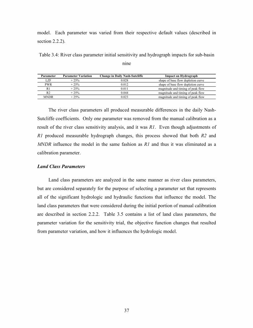
Table 3.4: River class parameter initial sensitivity and hydrograph impacts for sub-basin
nine
Parameter Parameter Variation Change in Daily Nash-Sutcliffe Impact on HydrographLZF + 25% 0.028 shape of base flow depletion curvePWR + 25% 0.012 shape of base flow depletion curve
R1 + 25% 0.011 magnitude and timing of peak flowR2 + 25% 0.044 magnitude and timing of peak flow
MNDR + 25% 0.023 magnitude and timing of peak flow
The river class parameters all produced measurable differences in the daily Nash-
Sutcliffe coefficients. Only one parameter was removed from the manual calibration as a
result of the river class sensitivity analysis, and it was R1. Even though adjustments of
R1 produced measurable hydrograph changes, this process showed that both R2 and
MNDR influence the model in the same fashion as R1 and thus it was eliminated as a
calibration parameter.
Land Class Parameters
Land class parameters are analyzed in the same manner as river class parameters,
but are considered separately for the purpose of selecting a parameter set that represents
all of the significant hydrologic and hydraulic functions that influence the model. The
land class parameters that were considered during the initial portion of manual calibration
are described in section 2.2.2. Table 3.5 contains a list of land class parameters, the
parameter variation for the sensitivity trial, the objective function changes that resulted
from parameter variation, and how it influences the hydrologic model.
38
Table 3.5: Land class parameter initial sensitivity and hydrograph impacts for sub-basin
nine
Parameter Parameter Variation Change in Daily Nash-Sutcliffe Impact on HydrographDS + 25% 0.000 no effect
DSFS + 25% 0.000 no effectRE + 25% 0.020 magnitude of peak flow (interflow based)AK + 25% 0.000 magnitude of peak flow (interflow based)
AKFS + 25% 0.000 magnitude of peak flow (interflow based)RETN + 25% 0.002 magnitude of peak flow (evaporation based)AK2 + 25% 0.013 magnitude of peak flow (interflow based)
AK2FS + 25% 0.003 magnitude of peak flow (interflow based)R3 + 25% 0.000 no effect
R3FS + 25% 0.000 no effectR4 + 25% 0.000 no effectCH + 25% 0.000 no effectMF + 25% 0.009 magnitude peak flow (melt based)
BASE + 0.1 0.009 timing of peak flow (melt based)RHO + 25% 0.000 total volume of flow (melt based)FTAL + 0.01 0.006 magnitude of peak flow (evapotranspiration based)
There are several parameters that have little to no effect on the modeling results
(DS, DSFS, AK, AKFS, R3, R3FS, R4, CH, and RHO) and were removed from the
manual calibration process. Of the seven remaining land class parameters that had a
higher impact on modeling results (RE, RETN, AK2, AK2FS, MF, BASE, and FTAL), the
RE, AK2, and AK2FS parameters were observed to have the same effect on the output
hydrographs. Since RE had a more significant effect on the daily Nash-Sutcliffe
coefficient, it was retained for the manual calibration and AK2 and AK2FS were removed
from the list of parameters to be further calibrated.
The parameters that were considered for further calibration were: LZF, PWR, R2,
MNDR, MF, BASE, RE, RETN, FTAL.
3.2.4 Manual Calibration Steps
This section outlines the method used during manual calibration. Using sub-basin nine as
an example, the parameters selected for manual calibration in section 3.2.3 are varied in a
specific order to improve the accuracy of the modeling results.

39
Starting with the pre-calibrated model the hydrograph and daily Nash-Sutcliffe
coefficient were analyzed for a specific basin. One of the sub-basins used during manual
calibration was sub-basin nine. A comparison of measured vs. modeled results with
default parameter values for sub-basin nine is shown in figure 3.8.
0
100
200
300
400
500
600
700
800
Year
Flow (m3/s)
MEASUREDMODELED
2002 2003 2004 2005
Figure 3.8: Measured streamflows vs. modeled streamflows from pre-calibrated model of
Red Deer River below Burnt Timber Creek (sub-basin 9)
The modeled hydrograph consistently predicted flows that were less than the
measured values. This was a result of both the magnitude of peak flows, and the shape of
the base flow depletion curves. The Nash-Sutcliffe daily coefficient for the pre-
calibrated sub-basin was -0.096. A general algorithm used to improve the hydrograph
manually for each sub-basin is described as follows:
1. Set initial parameters (default values) for all calibrated parameters
2. Run model and identify visually analyze for strengths and weaknesses in
the output hydrographs (magnitude of peak flows, etc)

40
3. Adjust base flow parameters (LZF, PWR) to improve the base flow
depletion curve using both visual hydrograph analysis and the results of
the objective function
4. Adjust streamflow parameters (R2, MNDR) to improve timing of peak
flows using both visual hydrograph analysis and the results of the
objective function
5. Focusing on the initial melt portions of the model outputs, adjust the snow
melt parameters (MF, BASE) to improve the timing and magnitude of the
peak flows resulting from snow melt using both visual hydrograph
analysis and the results of the objective function
6. Adjust remaining parameters (RE, RETN, FTAL) to improve magnitude of
all peak flows (those influenced by snow melt included) using primarily
the results of the objective function
Steps 2 – 6 were performed iteratively using small parameter adjustments to ensure
that certain land class parameters were not adjusted to hydrologically unrealistic values to
compensate for inadequacies in the default parameter values of other land classes.
The purpose of visual hydrograph inspection was that particularly in the early
stages of manual calibration, adjusting parameters that vary the timing of peak flows and
base flow depletion (LZF, PWR, R2, MNDR, MF, and BASE) sometimes lead to an
improved objective function, but a model that is further away from a reasonable
representation of historic hydrographs when visually inspected. The objective function is
not a perfect measure of model performance, and visual inspections help to ensure that
modeling improvements occur when the objective function improves as sometimes the
opposite can be the case. Since RE, RETN, and FTAL did not alter the timing of the
hydrographs they were manually adjusted using objective function results only (though
intermittent visual observations were still made to for validation). Adjusting only the
parameters selected in section 3.2.3 the manually calibrated hydrograph for sub-basin 9

41
produced a daily Nash-Sutcliffe coefficient of 0.738. The hydrograph is shown in figure
3.9.
0
100
200
300
400
500
600
700
800
Year
Flow (m3/s)
MEASUREDMODELED
2002 2003 2004 2005
Figure 3.9: Measured streamflows vs. modeled streamflows from manual calibration of
Red Deer River below Burnt Timber Creek (sub-basin 9)
While the monthly Nash-Sutcliffe coefficient was not considered during calibration,
it was used as a form of validation for the calibrated model. The monthly Nash-Sutcliffe
coefficient improved from -0.026 to 0.893.
The process of manual calibration was performed on each of the sub-basins shown
in table 3.3, each time focusing on the land and river class parameters that dominate those
basins respectively (shaded values). To complete the process of manually calibrating
four river class parameters for three river types, and five land class parameters for five
land types required approximately 2500 model runs.

42
3.2.5 Calibration Results
Manual calibration was performed on land class and river class parameters that had
significant effects on the sub-basins listed in table 3.3. Outputs from several sub-basins
with incomplete data sets were considered for the purpose of model validation.
Additionally, while the performance metric of the Nash-Sutcliffe monthly coefficient was
not used directly as a measure of accuracy, it was compared for the pre-calibrated and
manually calibrated models to provide another measure of model accuracy. The
parameter values found through manual calibration for each river class and land class
parameter described in section 3.2.3 are shown in table 3.6 and 3.7 respectively.
Table 3.6: River class parameter values obtained through manual calibration
1 2 3LZF 0.100E-04 0.100E-04 0.700E-04PWR 0.203E+01 0.100E+00 0.130E+00R2 0.200E+00 0.300E+01 0.100E+00
MNDR 0.100E+01 0.900E+01 0.100E+01
ParameterRiver Class
Table 3.7: Land class parameter values obtained through manual calibration
1 2 3 4 6RE 0.500E-01 0.200E-02 0.100E+00 0.200E+00 0.700E+00RETN 0.200E+02 0.700E+02 0.800E+02 0.700E+02 0.700E+02MF 0.100E+00 0.100E+00 0.100E+00 0.300E-01 0.100E+00BASE -0.200E+00 -0.100E+01 -0.100E+01 -0.300E+00 -0.100E+00FTAL 0.20 0.30 0.20 0.20 0.6
ParameterLand Class
To determine the success of manual calibration, results from sub-basins that were
not used to manually calibrate the model (sub-basins not in table 3.3) were considered.
Though these sub-basins did not have complete data sets, their Nash-Sutcliffe coefficients
were calculated by comparing only the data available with modeling results. The pre-
calibrated and manually calibrated values for the Nash-Sutcliffe daily and monthly
coefficients are shown in table 3.8. Shaded rows indicate sub-basins used to manually
calibrate the model.

43
Table 3.8: Pre-calibrated and manually calibrated Nash-Sutcliffe coefficients
Sub-basin Pre-Calibrated Manually Calibrated Improvement in Pre-calibrated Manually Calibrated Improvement in# Nash Daily Nash Daily Nash Daily? Nash Monthly Nash Monthly Nash Monthly?1 -0.181 0.621 YES -0.212 0.731 YES4 0.031 0.169 YES 0.115 0.377 YES5 -0.088 0.101 YES 0.234 0.605 YES6 0.482 -0.001 NO 0.714 0.902 YES7 0.094 0.425 YES 0.194 0.641 YES8 0.483 0.545 YES 0.325 0.835 YES9 -0.096 0.738 YES -0.026 0.893 YES16 0.410 0.619 YES 0.334 0.921 YES17 0.700 0.492 NO 0.653 0.931 YES19 -0.362 0.704 YES -0.078 0.907 YES20 0.265 0.779 YES 0.366 0.915 YES21 0.606 0.405 NO 0.591 0.778 YES22 0.468 0.503 YES 0.457 0.673 YES23 0.307 0.621 YES 0.269 0.743 YES25 -0.016 0.221 YES 0.244 0.329 YES26 -0.080 0.419 YES -0.028 0.552 YES27 -0.055 0.365 YES -0.146 0.470 YES28 0.272 0.065 NO 0.357 0.470 YES29 0.112 0.241 YES 0.118 0.534 YES
AVG/TOTAL 0.177 0.423 15 0.236 0.695 19
Though not all sub-basins were used during the manual calibration process, model
accuracy was improved for almost all cases. Since the calibrated parameters influence
modeling results watershed-wide, adjusting a parameter value to improve the results of
one sub-basin can change (hopefully improve but possibly degrade) modeling results in
other sub-basins. The model’s accuracy was improved for 15 of 19 sub-basins (7 of 9
validation sub-basins) for the daily Nash-Sutcliffe coefficient, and for 19 of 19 sub-basins
(9 of 9 validation basins) for the monthly Nash-Sutcliffe coefficient through automated
calibration. The average of both the Nash-Sutcliffe daily and monthly values also
increased significantly through manual calibration. Although the average values of the
objective function may not be the best way to evaluate the success of all hydrologic
calibrations it is effective in this case since each sub-basin (with the exception of sub-
basin 1) is a head water basin and is considered independently of all others. Another
option for comparing watershed-wide success would be a weighted average of the Nash-
Sutcliffe coefficients using sub-basin area, rainfall, streamflow, or another measure as the
weighting function. The objective function is weighted by average streamflow during the
automated calibration in the following section.

44
3.3 Automated Calibration
The purpose of using an automated algorithm to calibrate the model was to refine some
of the estimated parameter values found from manual calibration to improve model
results. While manual calibration was used to identify important parameters, automated
calibration searches the parameter space of some of those parameters to find the best
solution within the given parameter ranges. This section provides an outline of how the
manually calibrated model was improved using automated calibration. The method uses
an objective function that is calculated using the results from multiple sub-basins in each
trial. Described in this section is a brief description of the optimization algorithm
selected for this study, an outline of the parameter ranges used, the objective function
used, the selection of sub-basins, and results.
3.3.1 Optimization Algorithm (DDS)
The optimization algorithm chosen for this study is the dynamically dimensioned search
(DDS) (Tolson & Shoemaker, 2007). For DDS to function with WATFLOOD, it
requires a model parameter set, and the corresponding parameter ranges in terms of
maximum and minimum values. The DDS manual (Tolson & Seglenieks, 2007)
recommends that for optimization problems involving 10 or more parameters that 1000
function evaluations can typically generate reasonable results, so that will be the value
used for this study. Details on the specifics of the DDS algorithm can be found in
(Tolson & Shoemaker, 2007).
3.3.2 Parameter Selection & Parameter Ranges
The parameters selected for automated calibration are chosen with a goal of representing
the major hydrologic processes that heavily influence modeling results. Through the
manual calibration the dominant processes were found to be: snow melt, base flow

45
depletion, evapotranspiration, streamflow rates, evaporation, and interflow. The
parameters selected to represent each process are shown in table 3.9:
Table 3.9: Automated calibration parameters selected by hydrologic process
Hydrologic Process ParametersSnow Melt MF, BASEBaseflow Depletion LZFEvapotranspiration RETNStream Flow Rates R2Evaporation FTALInterflow RE
Each process was assigned one parameter for automated calibration except for snow
melt. For snow melt, two parameters were selected since both MF and BASE have
significantly different effects on the output hydrographs. Both PWR and MNDR were not
included in the automated calibration process because they influence the output
hydrographs in a very similar manner to LZF and R2 respectively, but less significantly
(table 3.4).
Initially, the range of each parameter was chosen as approximately +/- 50% of the
value obtained from manual calibration as long as that range does not exceed the
reasonable boundaries for the parameter which are governed by hydrologic and physical
limitations (i.e. MNDR cannot be less than 1). For BASE an initial range was selected as
+/- 1.5 degrees, and for FTAL, initial ranges were selected as +/- 0.2 (minimum of 0.01,
and maximum of 1.0).
Following each automatic calibration trial, the ranges for each parameter were reset
according to the results of the trial. Figure 3.10 depicts a decision diagram outlining how
parameters were adjusted after each trial.

46
Complete Automated Trial
Is new parameter value within 10% of range limit?
YES
NO
Automated calibration finished
Did objective function sufficiently improve?
(> 2%)
YES
Reset parameter range centered around new
parameter valueReduce range magnitude
by 50%
NO
Set initial parameter ranges
Figure 3.10: Automated calibration parameter adjustment flow chart
As shown above, trials will continue until the model does not show sufficient
improvement.
3.3.3 Objective Function Weighting Method
The objective function used for automated trials is a weighted sum of the Nash-Sutcliffe
daily coefficients based on the average flow from each sub-basin. The weighting
function is as follows:
∑
∑
=
== 3
1
1
*
bb
n
bbb
d
Q
QNN (3.2)
where Nd is the weighted Nash-Sutcliffe daily value used to evaluate the model, Nb is the
Nash-Sutcliffe daily value from each sub-basin involved in the calculation, and Qb is the
average measured flow for the calibration period from each sub-basin involved in the
calculation.

47
3.3.4 Sub-basin Selection
The sub-basins selected for automatic calibration were not the same set selected for
manual calibration. The purpose of this was to increase the number of sub-basins that
could be used as validation sub-basins to gain more information about the success of the
weighted objective function. The sub-basins used for the automated calibration objective
function calculation are selected from the sub-basins listed in table 3.3. The sub-basins
were chosen to represent all major land classes, and represent a variety of geographic
areas so that the automated algorithm calibrates to an objective function that represents
historic data from a variety of regions within the watershed. The sub-basins were also
chosen to have a full historic streamflow data set for the simulation period (January 1,
2002 to December 31, 2005). The sub-basins used in automated calibration are shown in
table 3.10 and figure 3.11.
Table 3.10: Sub-basins used for automated calibration
Sub-basin Area Dense Forest Light Forest Mixed Forest Open Wetland Agricultural Glacier Water Impervious# (sq km) % % % % % % % % %5 784 10.9 3.7 17.0 18.2 0.4 50.0 0.0 0.0 0.09 2418 36.8 15.1 1.4 34.9 7.3 0.0 3.0 1.5 0.016 321 22.4 14.4 50.3 10.8 1.2 0.0 0.2 0.9 0.020 777 13.1 26.1 21.6 35.4 3.1 0.0 0.4 0.1 0.023 630 13.1 7.8 31.3 19.7 2.4 23.5 1.1 1.3 0.025 233 62.9 15.3 5.1 13.9 2.6 0.0 0.0 0.3 0.0
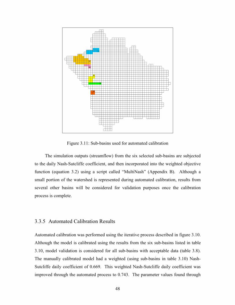
48
5
9
16
20
23
25
Figure 3.11: Sub-basins used for automated calibration
The simulation outputs (streamflow) from the six selected sub-basins are subjected
to the daily Nash-Sutcliffe coefficient, and then incorporated into the weighted objective
function (equation 3.2) using a script called “MultiNash” (Appendix B). Although a
small portion of the watershed is represented during automated calibration, results from
several other basins will be considered for validation purposes once the calibration
process is complete.
3.3.5 Automated Calibration Results
Automated calibration was performed using the iterative process described in figure 3.10.
Although the model is calibrated using the results from the six sub-basins listed in table
3.10, model validation is considered for all sub-basins with acceptable data (table 3.8).
The manually calibrated model had a weighted (using sub-basins in table 3.10) Nash-
Sutcliffe daily coefficient of 0.669. This weighted Nash-Sutcliffe daily coefficient was
improved through the automated process to 0.743. The parameter values found through

49
the automated calibration process for each river class and land class parameter described
in section 3.2.3 are shown in table 3.11 and 3.12 respectively.
Table 3.11: River class parameter values obtained through automated calibration
1 2 3LZF 0.110E-04 0.112E-04 0.706E-04R2 0.670E+00 0.329E+01 0.140E+00
ParameterRiver Class
Table 3.12: Land class parameter values obtained through automated calibration
1 2 3 4 6RE 0.520E-01 0.200E-02 0.820E-01 0.167E+00 0.728E+00RETN 0.166E+02 0.644E+02 0.830E+02 0.631E+02 0.755E+02MF 0.976E-01 0.128E+00 0.129E+00 0.316E-01 0.102E+00BASE -0.197E+00 -0.113E+01 -0.102E+01 -0.314E+00 -0.115E+00FTAL 0.22 0.32 0.25 0.12 0.72
ParameterLand Class
The automatic calibration was done using the weighted objective function as a
measure of model accuracy, and the parameter values found were applied across the
entire basin. Although the weighed objective function improved through automated
calibration, the success of the method is measured by considering modeling
improvements from the individual sub-basins in the model. Additionally, the Nash-
Sutcliffe monthly coefficients are used as performance metric since the automated
process measures considered only the daily measurements. The Nash-Sutcliffe daily and
monthly coefficients resulting from automated calibration are compared to the manually
calibrated values for all acceptable basins in table 3.13. Shaded rows indicate sub-basins
that were automatically calibrated.

50
Table 3.13: Nash-Sutcliffe coefficients from manual and automated calibrations
Sub-basin Manually Calibrated Automated Improvement in Manually Calibrated Automated Improvement in# Nash Daily Nash Daily Nash Daily? Nash Monthly Nash Monthly Nash Monthly?1 0.621 0.673 YES 0.731 0.768 YES4 0.169 0.293 YES 0.377 0.316 NO5 0.101 0.426 YES 0.605 0.782 YES6 -0.001 0.763 YES 0.902 0.911 YES7 0.425 0.422 NO 0.641 0.640 NO8 0.545 0.677 YES 0.835 0.830 NO9 0.738 0.768 YES 0.893 0.958 YES16 0.619 0.753 YES 0.921 0.968 YES17 0.492 0.559 YES 0.931 0.955 YES19 0.704 0.689 NO 0.907 0.878 NO20 0.779 0.814 YES 0.915 0.920 YES21 0.405 0.612 YES 0.778 0.841 YES22 0.503 0.618 YES 0.673 0.728 YES23 0.621 0.679 YES 0.743 0.777 YES25 0.221 0.653 YES 0.329 0.787 YES26 0.419 0.541 YES 0.552 0.708 YES27 0.365 0.286 NO 0.470 0.479 YES28 0.065 0.195 YES 0.470 0.447 NO29 0.241 0.228 NO 0.534 0.561 YESAVG 0.423 0.560 15 0.695 0.750 14
Although only six sub-basins were automatically calibrated, improvements were
made in the Nash-Sutcliffe daily and monthly coefficients in most cases. Automated
calibration improved the model accuracy for 15 of 19 sub-basins (9 of 13 validation sub-
basins) for the daily Nash-Sutcliffe coefficient, and for 14 of 19 sub-basins (8 of 13
validation sub-basins) for the monthly Nash-Sutcliffe coefficient. Although the weighted
average showed improvement, the method is validated by the improvement of the basins
that were not considered during the automated calibration.
Finally, the pre-calibrated model results were compared to the fully calibrated
(automated) results. The Nash-Sutcliffe daily and monthly coefficients resulting from
automated calibration were compared to the pre-calibrated model for all acceptable
basins in table 3.14. Shaded rows indicate sub-basins that were automatically calibrated.

51
Table 3.14: Nash-Sutcliffe coefficients from pre-calibrated and automatically calibrated
model
Sub-basin Pre-Calibrated Automated Improvement in Pre-calibrated Automated Improvement in# Nash Daily Nash Daily Nash Daily? Nash Monthly Nash Monthly Nash Monthly?1 -0.181 0.673 YES -0.212 0.768 YES4 0.031 0.293 YES 0.115 0.316 YES5 -0.088 0.426 YES 0.234 0.782 YES6 0.482 0.763 YES 0.714 0.911 YES7 0.094 0.422 YES 0.194 0.640 YES8 0.483 0.677 YES 0.325 0.830 YES9 -0.096 0.768 YES -0.026 0.958 YES16 0.410 0.753 YES 0.334 0.968 YES17 0.700 0.559 NO 0.653 0.955 YES19 -0.362 0.689 YES -0.078 0.878 YES20 0.265 0.814 YES 0.366 0.920 YES21 0.606 0.612 YES 0.591 0.841 YES22 0.468 0.618 YES 0.457 0.728 YES23 0.307 0.679 YES 0.269 0.777 YES25 -0.016 0.653 YES 0.244 0.787 YES26 -0.080 0.541 YES -0.028 0.708 YES27 -0.055 0.286 YES -0.146 0.479 YES28 0.272 0.195 NO 0.357 0.447 YES29 0.112 0.228 YES 0.118 0.561 YESAVG 0.177 0.560 17 0.236 0.750 19
The automated calibration using a multi-basin approach produced improved
modeling results relative to pre-calibrated results in 17 of 19 sub-basins for the daily
Nash-Sutcliffe coefficient and 19 of 19 sub-basins for the monthly Nash-Sutcliffe
coefficient.
3.4 Summary
The Upper South Saskatchewan River watershed was modeled in WATFLOOD and
calibrated to a daily Nash-Sutcliffe coefficient using both manual and automated
calibration. Figure 3.12, 3.13, and 3.14 display hydrographs from the pre-calibrated
model and those produced by manual and automated calibration respectively for sub-
basin 9.
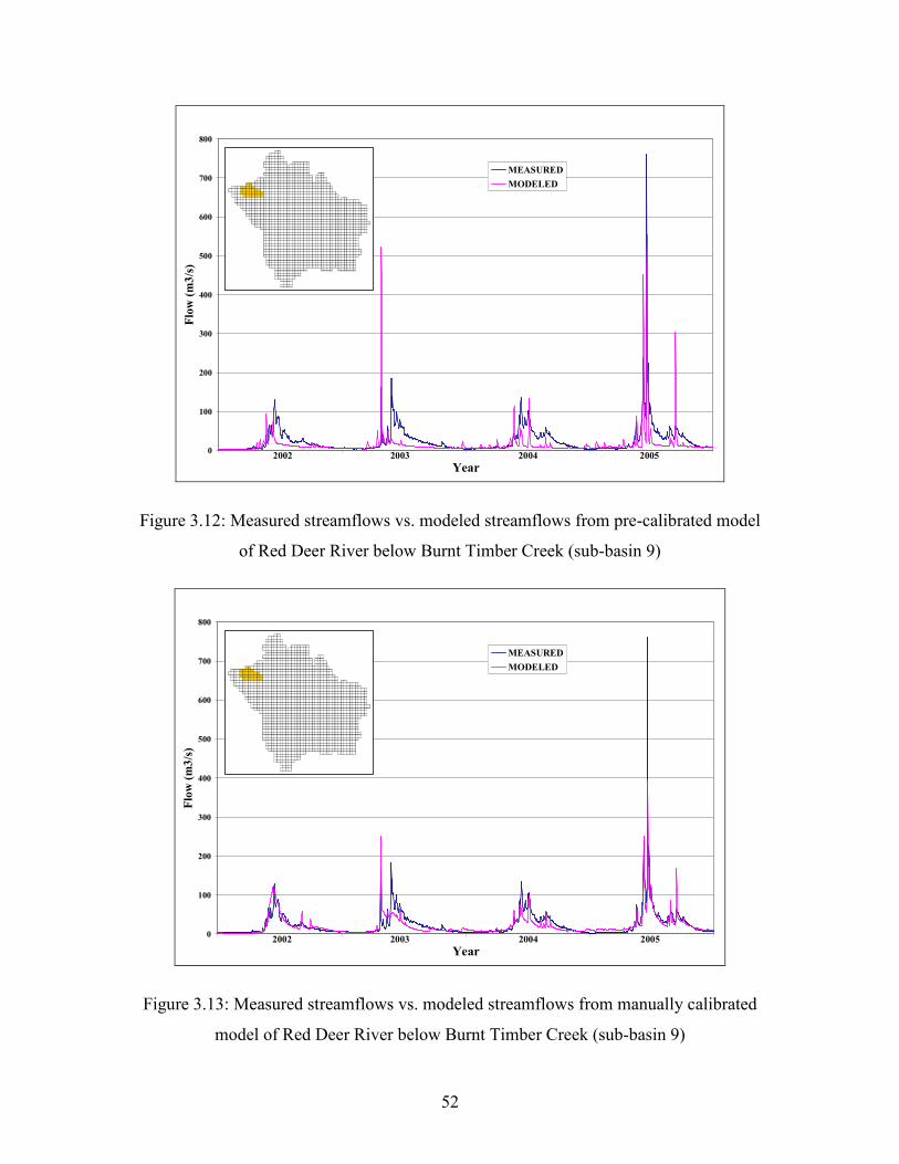
52
0
100
200
300
400
500
600
700
800
Year
Flow (m3/s)
MEASUREDMODELED
2002 2003 2004 2005
Figure 3.12: Measured streamflows vs. modeled streamflows from pre-calibrated model
of Red Deer River below Burnt Timber Creek (sub-basin 9)
0
100
200
300
400
500
600
700
800
Year
Flow (m3/s)
MEASUREDMODELED
2002 2003 2004 2005
Figure 3.13: Measured streamflows vs. modeled streamflows from manually calibrated
model of Red Deer River below Burnt Timber Creek (sub-basin 9)

53
0
100
200
300
400
500
600
700
800
Year
Flow (m3/s)
MEASUREDMODELED
2002 2003 2004 2005
Figure 3.14: Measured streamflows vs. modeled streamflows from automated calibration
of Red Deer River below Burnt Timber Creek (sub-basin 9)
Calibration was successful in that manual calibration produced improved modeling
results in 15 of 19 sub-basins for the daily Nash-Sutcliffe coefficient and 19 of 19 sub-
basins for the monthly Nash-Sutcliffe coefficient. Automated calibration using a multi-
basin approach produced improved modeling results relative to manually calibrated
results in 15 of 19 sub-basins for the daily Nash-Sutcliffe coefficient and 14 of 19 sub-
basins for the monthly Nash-Sutcliffe coefficient. The automated calibration using a
multi-basin approach produced improved modeling results relative to pre-calibrated
results in 17 of 19 sub-basins for the daily Nash-Sutcliffe coefficient and 19 of 19 sub-
basins for the monthly Nash-Sutcliffe coefficient.
The approach was very effective in improving modeling results over the entire
watershed, producing consistent improvements in almost all of the sub-basins used for
validation. There are several potential improvements that could be made to improve the
calibration. First, more parameters could be included in the automatic calibration
process. Although this would provide the opportunity for a more accurate model, but it
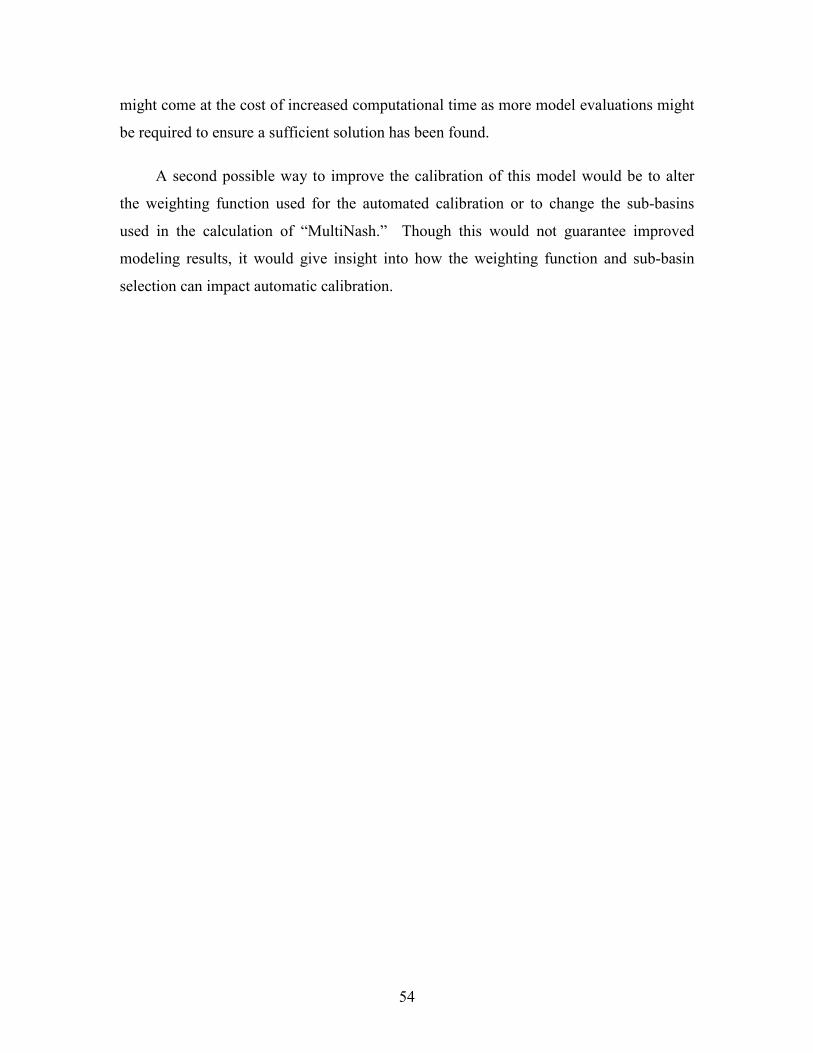
54
might come at the cost of increased computational time as more model evaluations might
be required to ensure a sufficient solution has been found.
A second possible way to improve the calibration of this model would be to alter
the weighting function used for the automated calibration or to change the sub-basins
used in the calculation of “MultiNash.” Though this would not guarantee improved
modeling results, it would give insight into how the weighting function and sub-basin
selection can impact automatic calibration.

55
Chapter 4
Impacts of Precipitation De-clustering
The first portion of this thesis dealt with hydrologic model calibration using both manual
and automated calibration methods. This chapter applies the automatic calibration
methodology to four models, each with a precipitation data set that has been reduced
from the original set used in chapter 3. The first goal of this chapter is to determine how
removing specific rain gauges from the precipitation data set affected the calibration
potential of hydrologic models on both the local (sub-basin) and global (regional scale
watershed). The results of this study will not only provide information on the effects of
removing precipitation data, it is intended to provide insight into the potential to improve
hydrologic models by increasing the number and/or density of available meteorological
stations. Results from areas of the watershed with different spatial distributions of
precipitation gauges are also analyzed in an attempt to determine a relationship between
rain-gauge density and calibrated Nash-Sutcliffe coefficients.
The second goal of this portion of the study was to observe how parameter values
vary from the “optimum” values found from calibrating the model described in chapter 3.
Comparing how each parameter varies when the precipitation inputs are changed will
reveal how uncertainty in precipitation translates to potential uncertainty in different
parameter values.
The rain gauge data set that was used to produce the input precipitation data for the
model was reduced several times through a de-clustering method. Each time the rain
gauge set was reduced, a new input data set was interpolated (using equation 2.2 and 2.3)
and the model was re-calibrated using the method outlined in Chapter 3.
The results of this study will help to determine how removing precipitation data
points impacts hydrologic modeling calibrations. It will help to determine areas of
regional scale hydrologic models that require more precipitation gauges and areas that
56
can have use a reduced data set without significantly decreasing the accuracy of modeling
results.
4.1 De-clustering Method
De-clustering is the process of removing data points in an effort to improve the spatial
distribution of the data. De-clustering of the precipitation data reduces rain gauge density
and provides a rain gauge set that is used to create a new interpolation to be used as an
input data set.
4.1.1 Rain Gauge Removal Order
Starting with a set of rain gauges that included all 28 gauges in the study area, a
clustering index was calculated using a variation on the nearest neighbour removal order
(Ahrens, 2005) according to:
∑=
=N
iidCI
1
2 (4.1)
where CI is the clustering index, di is the distance between the selected rain gauge and the
closest neighboring rain gauge and N is the number of neighboring rain gauges used to
calculate CI. For each rain gauge, di is calculated for the closest N (4 for this study)
neighboring rain gauges and the gauge with lowest CI is removed and the process is
repeated. An example of how CI values would be calculated is shown in section 2.1.4.
The order of removal of the 28 rain gauges according to equation 4.1 is shown in
table 4.1.

57
Table 4.1 – Rain gauge removal order
Gauge CI17 1.36E+031 2.14E+0322 3.91E+0314 4.09E+0313 5.62E+039 6.50E+0319 6.55E+0327 9.68E+0310 1.02E+046 1.34E+0426 1.35E+0411 1.76E+048 2.36E+047 3.82E+0412 4.21E+0428 5.80E+0424 8.07E+0421 9.68E+0415 1.35E+053 1.78E+0520 1.98E+0525 3.06E+054 4.71E+0523 9.06E+05
2 N/A16 N/A5 N/A18 N/A
The final four gauges (2, 16, 5, and 18) listed above do not have a clustering index
because at least four other gauges are required for this calculation.
4.1.2 De-clustering Trials
De-clustering of the initial rain gauge set was done four times. Each trial removed five
rain gauges (including those removed in previous trials). Table 4.2 shows summarizes
the gauges removed each step.

58
Table 4.2: Rain gauges removed for each de-clustering trial
Trial Gauges Removed23 Gauges 17, 1, 22, 14, 1318 Gauges 9, 19, 27, 10, 613 Gauges 26, 11, 8, 7, 128 Gaugues 28, 24, 21, 15, 3
The rain gauge sets were interpolated to generate precipitation data for each grid
cell according to the IDW interpolation method outlined in section 2.1.3 (equation 2.2
and 2.3), with a maximum search radius implemented according to Shepard’s method
(Yoeli, 1975). The search radius selected for this interpolation was 100 km, and the
minimum number of points required for the interpolation was 1.
The locations of the rain gauges used in the complete set (used for calibration in
chapter 3) are compared to the rain gauge sets used in the de-clustering trials in figure 4.1
(a – e).

59
(a)
(b)
(c)
(d)
(e)
Figure 4.1: Rain gauges used for de-clustering trials (a) Complete rain gauge set; (b) Trial
1 rain gauge set; (c) Trial 2 rain gauge set; (d) Trial 3 rain gauge set; (e) Trial 5 rain
gauge set

60
4.2 Calibration Results
Once the interpolation for the rain gauge set was complete, the model was run with the
new precipitation interpolations used as the input data set. The parameter values for this
first model run were the final parameter values from the automated calibration (Table
3.11 and 3.12).
The initial Nash-Sutcliffe daily and monthly coefficients for each de-clustering trial
are shown in table 4.3 and 4.4 respectively.
Table 4.3: Initial daily Nash-Sutcliffe coefficients for de-clustering models
Sub-basin Full Set Calibrated Trial 1 Pre-calibrated Trial 2 Pre-calibrated Trial 3 Pre-calibrated Trial 4 Pre-calibrated# Nash Daily Nash Daily Nash Daily Nash Daily Nash Daily1 0.673 0.598 0.653 0.276 0.0334 0.293 0.320 0.295 0.290 0.1035 0.426 0.342 0.526 0.168 -0.1546 0.763 0.550 0.736 0.236 -0.2317 0.422 0.427 0.368 0.400 0.0058 0.677 0.665 0.596 0.629 -0.3649 0.768 0.763 0.757 0.757 0.14716 0.753 0.737 0.658 0.633 -0.46717 0.559 0.445 0.355 0.321 -0.35319 0.689 -0.569 0.502 0.183 -0.61220 0.814 0.748 0.650 0.658 0.27821 0.612 0.475 0.420 0.402 -0.32922 0.618 0.543 0.530 0.517 0.27423 0.679 0.608 0.605 0.605 0.39925 0.653 0.628 0.637 0.637 0.41826 0.541 0.502 0.498 0.502 0.14227 0.286 0.228 0.228 0.221 -0.21428 0.195 0.189 0.313 0.313 0.00029 0.228 0.224 0.308 0.308 0.265AVG 0.560 0.443 0.507 0.424 -0.035

61
Table 4.4: Initial monthly Nash-Sutcliffe coefficients for de-clustering models
Sub-basin Full Set Calibrated Trial 1 Pre-calibrated Trial 2 Pre-calibrated Trial 3 Pre-calibrated Trial 4 Pre-calibrated# Nash Monthly Nash Monthly Nash Monthly Nash Monthly Nash Monthly1 0.768 0.655 0.754 0.317 0.2274 0.316 0.398 0.354 0.437 0.2925 0.782 0.661 0.845 0.572 0.0276 0.911 0.811 0.844 0.435 -0.1517 0.640 0.648 0.545 0.604 -0.0878 0.830 0.860 0.676 0.766 -0.2239 0.958 0.953 0.945 0.948 0.14516 0.968 0.960 0.825 0.796 -0.49917 0.955 0.915 0.657 0.716 -0.10819 0.878 0.381 0.682 0.515 0.59620 0.920 0.829 0.783 0.818 0.65721 0.841 0.726 0.754 0.744 -0.30422 0.728 0.693 0.684 0.673 0.57423 0.777 0.726 0.719 0.721 0.71925 0.787 0.766 0.774 0.774 0.60626 0.708 0.679 0.678 0.680 0.60827 0.479 0.448 0.446 0.444 0.53328 0.447 0.447 0.507 0.507 0.66229 0.561 0.556 0.600 0.600 0.661AVG 0.750 0.690 0.688 0.635 0.260
As may be expected, the general trend of the pre-calibrated models was a decreased
Nash-Sutcliffe coefficient as the number of rain gauges used to interpolate the input data
was reduced. Starting from each pre-calibrated model, each of the models was calibrated
using automated calibration as described in section 3.3.
Automated calibration identified unique parameter sets for each model with de-
clustered input data sets. Parameter variation was tracked for each river and land class
parameter to determine how they varied from the “optimal” values that were found from
calibration of the complete data set. Figure 4.2 shows the parameter variation of the river
class parameters (LZF and R2) from the de-clustering trials.

62
0.E+00
1.E-05
2.E-05
3.E-05
4.E-05
5.E-05
6.E-05
7.E-05
8.E-05
LZF
Full Set
Trial 1
Trial 2
Trial 3
Trial 4
RC1 RC2 RC3
0.0
0.5
1.0
1.5
2.0
2.5
3.0
3.5
4.0
R2
Full Set
Trial 1
Trial 2
Trial 3
Trial 4
RC1 RC2 RC3
Figure 4.2: River class parameter variation resulting from de-clustering trials
The values of LZF and R2 found through automated calibration of the de-clustered
models were all very similar. The river class parameters LZF and R2 control the base
flow depletion curve and the timing of the peak flows. It was expected that these values
would not vary significantly when a de-clustered precipitation set was used as the model
input since they have already been calibrated to match the shape of the base flow
depletion curve (LZF), and the timing of the peak flows (R2) of the historic data set.
They have very little to do with modeled runoff volume which is where most of the
uncertainty in the de-clustered models comes from.
Land class parameters control the magnitude of the peak flows and the volume of
runoff simulated by WATFLOOD. Different interpolations would likely lead to different
volumes of input precipitation, and thus, variation of the land class parameters optimize
the Nash-Sutcliffe coefficients was expected. Figure 4.3 shows the parameter variation
of the land class parameters (RE, RETN, MF, BASE, and FTAL) from the de-clustering
trials.

63
0.0
0.1
0.2
0.3
0.4
0.5
0.6
0.7
0.8
0.9
1.0
RE
Full SetTrial 1Trial 2
Trial 3Trial 4
LC1 LC2 LC4LC3 LC6
0
20
40
60
80
100
120
140
160
180
RETN
Full Set
Trial 1Trial 2Trial 3Trial 4
LC1 LC2 LC4LC3 LC6
0.0
0.1
0.1
0.2
0.2
0.3
0.3
0.4
MF
Full Set
Trial 1Trial 2Trial 3Trial 4
LC1 LC2 LC4LC3 LC6
-1.5
-1.0
-0.5
0.0
0.5
1.0
1.5
BASE
Full Set
Trial 1Trial 2
Trial 3Trial 4
LC1 LC2 LC4LC3 LC6
0.0
0.1
0.2
0.3
0.4
0.5
0.6
0.7
0.8
FTAL
Full Set
Trial 1Trial 2
Trial 3Trial 4
LC1 LC2 LC4LC3 LC6
Figure 4.3: Land class parameter variation resulting from de-clustering trials

64
Compared to the river class parameters, the de-clustered models produced more
variation in the land class parameter values. The variation of the land class parameters
was within a reasonable range, with all parameters having variation less than one order of
magnitude, and with BASE having no variation more than two degrees Celsius.
The initial and calibrated weighted daily Nash-Sutcliffe coefficients for each trial
are shown in table 4.5.
Table 4.5: Initial and calibrated weighted daily Nash-Sutcliffe coefficients for de-
clustering trials
Trial Full Set Calibrated Trial 1 Trial 2 Trial 3 Trial 4Numer of Gauges 28 23 18 13 8Initial Weighted Daily Nash 0.669 0.711 0.693 0.676 0.174Calibrated Weighted Daily Nash 0.743 0.732 0.721 0.714 0.315
Although the weighted daily Nash-Sutcliffe coefficients were improved for each
trial through automated calibration, analysis of the results for each sub-basin was
required to determine how precipitation de-clustering impacts modeling results on a local
and global scale. Table 4.6 and 4.7 show the daily and monthly Nash-Sutcliffe
coefficients respectively for each trial for each sub-basin. The shaded values indicate the
best result for each sub-basin.
Table 4.6: Calibrated daily Nash-Sutcliffe coefficients for each de-clustering trial
Sub-basin Full Set Calibrated Trial 1 Calibrated Trial 2 Calibrated Trial 3 Calibrated Trial 4 Calibrated# Nash Daily Nash Daily Nash Daily Nash Daily Nash Daily1 0.673 0.616 0.670 0.400 0.1284 0.293 0.237 0.298 0.222 0.0015 0.426 0.409 0.596 0.384 0.1136 0.763 0.481 0.732 0.380 0.0067 0.422 0.438 0.415 0.373 0.0668 0.677 0.633 0.610 0.633 -0.0799 0.768 0.783 0.778 0.791 0.27716 0.753 0.720 0.665 0.610 -0.25517 0.559 0.420 0.364 0.366 -0.05619 0.689 -0.465 0.542 0.279 0.15220 0.814 0.785 0.704 0.719 0.45321 0.612 0.428 0.410 0.423 -0.07222 0.618 0.523 0.542 0.513 0.40223 0.679 0.616 0.637 0.616 0.54025 0.653 0.617 0.613 0.565 0.32626 0.541 0.538 0.541 0.564 0.43827 0.286 0.209 0.217 0.329 0.42228 0.195 0.188 0.296 0.337 0.19229 0.228 0.221 0.318 0.338 0.423AVG 0.560 0.442 0.524 0.466 0.183
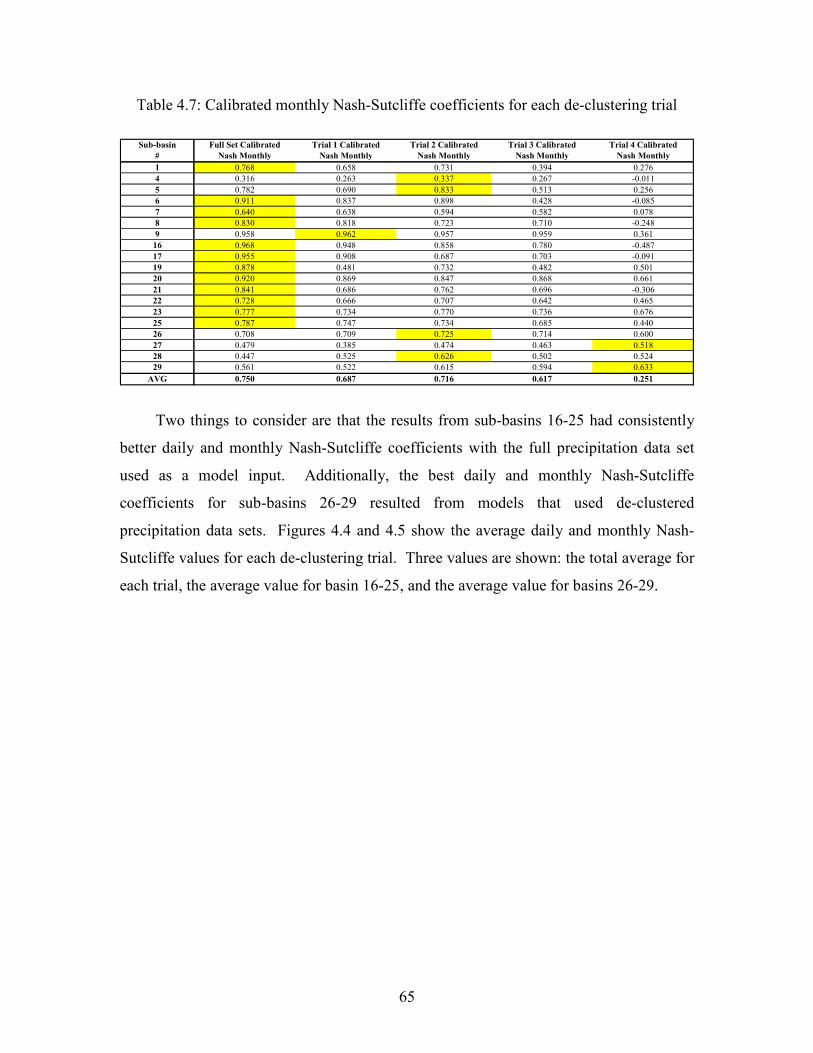
65
Table 4.7: Calibrated monthly Nash-Sutcliffe coefficients for each de-clustering trial
Sub-basin Full Set Calibrated Trial 1 Calibrated Trial 2 Calibrated Trial 3 Calibrated Trial 4 Calibrated# Nash Monthly Nash Monthly Nash Monthly Nash Monthly Nash Monthly1 0.768 0.658 0.731 0.394 0.2764 0.316 0.263 0.337 0.267 -0.0115 0.782 0.690 0.833 0.513 0.2566 0.911 0.837 0.898 0.428 -0.0857 0.640 0.638 0.594 0.582 0.0788 0.830 0.818 0.723 0.710 -0.2489 0.958 0.962 0.957 0.959 0.36116 0.968 0.948 0.858 0.780 -0.48717 0.955 0.908 0.687 0.703 -0.09119 0.878 0.481 0.732 0.482 0.50120 0.920 0.869 0.847 0.868 0.66121 0.841 0.686 0.762 0.696 -0.30622 0.728 0.666 0.707 0.642 0.46523 0.777 0.734 0.770 0.736 0.67625 0.787 0.747 0.734 0.685 0.44026 0.708 0.709 0.725 0.714 0.60027 0.479 0.385 0.474 0.463 0.51828 0.447 0.525 0.626 0.502 0.52429 0.561 0.522 0.615 0.594 0.633AVG 0.750 0.687 0.716 0.617 0.251
Two things to consider are that the results from sub-basins 16-25 had consistently
better daily and monthly Nash-Sutcliffe coefficients with the full precipitation data set
used as a model input. Additionally, the best daily and monthly Nash-Sutcliffe
coefficients for sub-basins 26-29 resulted from models that used de-clustered
precipitation data sets. Figures 4.4 and 4.5 show the average daily and monthly Nash-
Sutcliffe values for each de-clustering trial. Three values are shown: the total average for
each trial, the average value for basin 16-25, and the average value for basins 26-29.

66
0.0
0.1
0.2
0.3
0.4
0.5
0.6
0.7
0.8
Nash Daily
Number of Gauges
Average Daily Nash (Complete Set)Average Daily Nash (Gauge 16-25)Average Daily Nash (Gauge 26-29)
28 23 18 13 8
Figure 4.4: Daily Nash-Sutcliffe values from de-clustering trials
0.0
0.1
0.2
0.3
0.4
0.5
0.6
0.7
0.8
0.9
Nash Monthly
Number of Gauges
Average Monthly Nash (Complete Set)Average Monthly Nash (Gauge 16-25)Average Monthly Nash (Gauge 26-29)
28 23 18 13 8
Figure 4.5: Monthly Nash-Sutcliffe values from de-clustering trials
Figures 4.6 and 4.7 show the locations of sub-basins 16-25, and 26-29 respectively
with and overlay of the locations of the full rain gauge set.
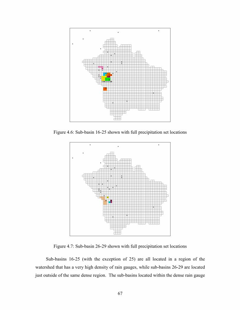
67
R RR
R
R
R
RR
R
R RR R
R16
R RR
17 R RR 20 R 19R R 21
R22
R 23
25
R
RR
Figure 4.6: Sub-basin 16-25 shown with full precipitation set locations
R RR
R
R
R
RR
R
R RR R
R
R RR
R RR RR R
R
R27
26 2829
R
RR
Figure 4.7: Sub-basin 26-29 shown with full precipitation set locations
Sub-basins 16-25 (with the exception of 25) are all located in a region of the
watershed that has a very high density of rain gauges, while sub-basins 26-29 are located
just outside of the same dense region. The sub-basins located within the dense rain gauge
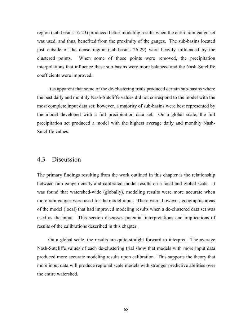
68
region (sub-basins 16-23) produced better modeling results when the entire rain gauge set
was used, and thus, benefited from the proximity of the gauges. The sub-basins located
just outside of the dense region (sub-basins 26-29) were heavily influenced by the
clustered points. When some of those points were removed, the precipitation
interpolations that influence these sub-basins were more balanced and the Nash-Sutcliffe
coefficients were improved.
It is apparent that some of the de-clustering trials produced certain sub-basins where
the best daily and monthly Nash-Sutcliffe values did not correspond to the model with the
most complete input data set; however, a majority of sub-basins were best represented by
the model developed with a full precipitation data set. On a global scale, the full
precipitation set produced a model with the highest average daily and monthly Nash-
Sutcliffe values.
4.3 Discussion
The primary findings resulting from the work outlined in this chapter is the relationship
between rain gauge density and calibrated model results on a local and global scale. It
was found that watershed-wide (globally), modeling results were more accurate when
more rain gauges were used for the model input. There were, however, geographic areas
of the model (local) that had improved modeling results when a de-clustered data set was
used as the input. This section discusses potential interpretations and implications of
results of the calibrations described in this chapter.
On a global scale, the results are quite straight forward to interpret. The average
Nash-Sutcliffe values of each de-clustering trial show that models with more input data
produced more accurate modeling results upon calibration. This supports the theory that
more input data will produce regional scale models with stronger predictive abilities over
the entire watershed.

69
On a local scale, the results shown in this chapter are more complex. Since some
sub-basins had the best Nash-Sutcliffe coefficients from de-clustered models, the results
require more interpretation. It should be noted that some of the more complex results
might be due to poor optimizer performance as the calibration method used is not perfect
(nor is any). Additional optimization trials might lead to significantly better results. The
sub-basins previously shown in figure 4.7 are all located in a geographic region with a
low local rain gauge density and no rain gauges actually lie within the sub-basin
boundaries. The best modeling results were produced by using a de-clustered data set. If
this study was done in reverse (i.e. starting with 8 rain gauges and increasing to 28), no
rain gauges are added within the sub-basin limits, and thus, there is no guarantee that
more data would improve modeling results.
The sub-basins previously shown in figure 4.6, which are located in a region with a
higher local rain gauge density, suffered from de-clustering. Again, if the study was
performed in reverse, several rain gauges would have been added within the limits of the
displayed sub-basins, and improved modeling results would have been expected.
The local rain gauge density in this study was found to be very important to
modeling results when the rain gauges were within the limits of the sub-basin being
modeled. When rain gauges are added outside the limits of a sub-basin, it is very difficult
to predict the effect it will have on modeling results.
This case study shows that portions of the model (sub-basins 26-29) with low local
rain gauge density can still produce reasonably accurate results (0.33 to 0.56 daily Nash-
Sutcliffe coefficients for this study as shown in table 4.6); however, sub-basins located
within geographic regions of higher rain gauge density (sub-basins 16-25) produced
significantly better and more consistent results (0.56 to 0.81 daily Nash-Sutcliffe
coefficients as shown in table 4.6). For a regional scale model it would be very difficult
to trust modeling results fuelled by a scarce data set regardless of the quality of the
model’s predictive power. With good values determined for the river class parameters,
the uncertainty in precipitation mainly translates to uncertainty in the land class
70
parameter values and can offset inaccurate precipitation input data produced by poor
local rain gauge density.
The results presented in this chapter are difficult to generalize to hydrologic models
in general, as the site was quite data poor with respect to available rain gauge data.
Without using an initial data set that contains consistently spaced rain gauges, the
importance of the rain gauge density for each trial can be very difficult to interpret. The
ideal scenario to test the effects of de-clustering would involve having a rain gauge
located in every grid cell in the study area. Gauges would then be removed according to
equation 4.1, and the model would be re-calibrated. Starting off the scenario with equally
spaced rain gauges would give more importance to the rain gauge density values when
compared to the resulting Nash-Sutcliffe coefficients of each de-clustered model.
A limitation that is always present in hydrologic modeling is the error in the
recorded historic precipitation data at each individual rain gauge, and this error can be
compounded when less data is available. While each rain gauge is likely to have some
error in each recorded precipitation event, the errors in models with a high density of data
points can even each other out when spatially interpolated. With a low density model
that essentially becomes subjected to a nearest neighbour interpolation, huge portions of
the model are fuelled by an input that is based on only one rain gauge that may have
significant error. The potential for this compounded error is another reason why models
with low rain gauge density are very difficult to trust.
The value of an added data point is only as good as the proximity it has to the sub-
basin being studied. In a regional scale model, with many sub-basins there are bound to
be geographic locations of the watershed that are relatively data-poor with regards to rain
gauge availability. To trust the results of a regional scale model that has parameter
flexibility similar to the WATFLOOD model used in this case study, the local rain gauge
density must be sufficient and at least partially within the boundaries of the sub-basins
considered. Though there is evidence that some data points can be removed without
significantly decreasing modeling accuracy in geographic locations with high rain gauge

71
density, the results of this chapter show that the best results for a regional scale model
will come from using all available precipitation inputs.

72
Chapter 5
Summary
This primary purpose of this thesis was to present a general approach to calibrating a
regional scale hydrologic model using a WATFLOOD model of the upper South
Saskatchewan River watershed as a case study. Initially, manual calibration was
described and performed on several sub-basins within the watershed. Using the manual
calibration results as a basis for automated calibration, a multi-basin automated
calibration approach was developed and applied to the model. The results demonstrated
that both methods were effective tools for improving modeling results. Not only were the
daily Nash-Sutcliffe coefficients of the sub-basins subjected to calibration all improved,
the results from x of y sub-basins used for validation were also improved. Additionally,
improvement in the monthly Nash-Sutcliffe coefficient was observed for every sub-basin
in the calibrated model relative to the pre-calibrated model. Overall, the average daily
Nash-Sutcliffe coefficient of the 19 calibration and validation sub-basins improved from
an initial value of 0.17 before calibration to 0.43 after manual calibration and then to 0.56
after refinements with automatic calibration.
The calibration method was applied to four models that used de-clustered
precipitation data as their input with the purpose of determining the effects of rain gauge
density on modeling results. The results of the four calibrations, based on the daily and
monthly Nash-Sutcliffe coefficients of all 19 sub-basins, were compared to the initial
calibrated model that used the entire precipitation data set. Of the 19 sub-basins
considered, 11 of had the best daily Nash-Sutcliffe coefficients in the model that used the
entire precipitation data set, and the best values for the remaining 8 sub-basins were
produced from a de-clustered model.
Calibration of the de-clustered models produced almost no variation in the river
class parameters from the values found during the calibration of the initial model.
Variation was found in the land class parameter values, but it was within a reasonable
73
range, with optimal parameters being modified less than one order of magnitude from
their original values. Because the variation in the river class parameters was so low
compared to the land class parameters, future de-clustering studies should consider
placing a priority on re-calibrating land class parameters and not river class parameters.
De-clustered models create uncertainty in precipitation volume which translates to
uncertainty in land class parameter values since they have a much higher influence on
runoff volumes than river class parameters.
In general, models that used more input data produced better modeling results than
de-clustered models; however, de-clustered models did produce better results in some
cases. Because the variation of the parameter values was within reasonable ranges for
each of these improved cases, extended study into the effects of precipitation gauge
density on modeling accuracy may provide stronger conclusions on how input
precipitation data can be modified or supplemented to improve modeling results.

74
References Ahrens, B. (2005). Distance in spatial interpolation of daily rain gauge data. Hydrology
and Earth System Sciences Discussions, 2, 1893-1923.
Allen, R. J. & DeGaetano, A. T. (2005). Areal Reduction Factors for Two Eastern
United States Regions with High Rain-Gauge Density. Journal of Hydrologic
Engineering, 10:4, 327-335.
ArcInfo. (1991). Cell-based modelling with GRID. Environmental Systems Research
Institute, Inc., Redlands, USA.
Bedient, P. & Huber, W. (2002). Hydrology and Floodplain Analysis. New Jersey:
Prentice Hall.
Beven, K. J. & Hornberger, G. M. (1982). Assessing the effect of spatial pattern of
precipitation in modelling streamflow hydrograph. Water Resources Bulletin, 18,
823-829.
Beven, K. (2000). Uniqueness of place and process representations in hydrological
modeling. Hydrology and Earth System Sciences, 4(2), 203-213.
Boyle, P. D., Gupta, V. H. & Sorooshian, S. (2000). Toward improved calibration of
hydrologic models: Combining the strengths of manual and automatic method.
Water Resources Research, Vol. 36, No. 12, 3663-3674
Clark, I. (1979). Practical Geostatistics. London: Applied Science Publishers.
Cooper, V. A., Nguyen, V. T. V. & Nicell, J. A. (1997). Evaluation of global
optimization methods for conceptual rainfall-runoff model calibration. Water
Science and Technology, 36 (5), 53-60.
Crawford, N. H. & Burges, S. J. (2004). History of the Stanford Watershed Model.
Water Resources Impact, Volume 6, Number 2, 3-5.

75
Crawford, N. H. & Linsley, R. K. (1966). Digital Simulation in Hydrology: Stanford
Watershed Model IV. Technical Report No. 39, Department of Civil Engineering,
Stanford University, p. 210.
Debo, T. N. & Reese, A. J. (2002). Municipal Stormwater Management, 2nd edition.
Lewis Publishers.
Dent, M. C., Lynch, S. D. & Schulze, R. E. (1988). Mapping mean annual and other
rainfall statisitics over Southern Africa. University of Natal, Department of
Agricultural Engineering.
Donald, J.R. (1992). Snowcover depletion curves and satellite snowcover estimates for
snowmelt runoff modelling. Ph.D. Thesis, University of Waterloo, ON, Canada,
232 p.
Dorninger, M. Schneider, S. & Steinacker, R. (2008). On the interpolation of
precipitation data over complex terrain. Meteorology and Atmospheric Physics,
101, 175-189.
Duan, Q., Gupta, V., & Sorooshian, S. (1993). A shuffled complex evolution approach
for effective and efficient optimization. Journal of Optimization Theory and
Applications, 76, 501-521.
Environment Canada. (2007a). Real-Time Hydrometric Data.
http://scitech.pyr.ec.gc.ca/waterweb/formNav.asp (retrieved May, 2007).
Environment Canada. (2007b). Hourly Observation Data.
http://www.climate.weatheroffice.ec.gc.ca/climateData/canada_e.html (retrieved
May, 2007).
Fang, X., Minke, A., Pomeroy, J., Brown, T., Westbrook, C., Guo, X. & Guangul, S.
(2007). A Review of Canadian Prairie Hydrology: Principles, Modeling and
Response to Land Use and Drainage Change. Centre for Hydrology Report,
University of Saskatchewan.

76
Fenicia, F., Solomatine, D. P., Savenije, H. H. G. & Matgen, P. (2007). Soft combination
of local models in a multi-objective framework. Hydrology and Earth System
Sciences, 11, 1797-1809.
Franchini, M., Galeati, G. & Berra, S. (1998). Global optimization techniques for the
calibration of conceptual rainfall-runoff models. Hydrological Sciences Journal, 43
(3), 443-458.
Gan, T. Y., & Biftu, G. F. (1996). Automatic calibration of conceptual rainfall-runoff
models: optimization algorithms, catchment conditions, and model structure. Water
Resources Research, 32 (12), 3513-3524.
Government of Alberta Environment. (2009). Environment: South Saskatchewan River
Basin Water Information Portal. http://ssrb.environment.alberta.ca (retrieved May,
2009).
Jain, K. S. & Sudheer, K. P. (2008). Fitting of Hydrologic Models: A Close Look at the
Nash-Sutcliffe Index. Journal of Hydrologic Engineering, 10, 981-986.
Johnson, R. (2000). Miller & Freund’s Probability and Statistics for Engineers. New
Jersey: Prentice Hall.
Kouwen, N. (2007). WATFLOOD/WATROUTE Hydrologic Model Routing & Flow
Forecasting System. University of Waterloo, Department of Civil Engineering.
Kuczera, G. (1997). Efficient subspace probabilistic parameter optimization for
catchment models. Water Resources Research, 33 (1), 177-185.
Lynch, S. D. & Schulze, R. E. (1995). Techniques for Estimating Areal Daily Rainfall.
University of Natal, Department of Agricultural Engineering.
MacFarlane, A. & Tuson, A. (2008). Local search: A guide for the information retrieval
practitioner. Information and Processing Management, 45, 159-174.

77
Madsen, H. (2000). Automatic calibration of a conceptual rainfall-runoff model using
multiple objectives. Journal of Hydrology, 235, 276-288.
Madsen, H. (2003). Parameter estimation in distributed hydrological catchment
modeling using automatic calibration with multiple objectives. Advances in Water
Resources, 26, 205-216.
Madsen, H. & Wilson, G., Ammentorp, H. C., (2002). Comparison of different
automated strategies for calibration of rainfall-runoff models. Journal of
Hydrology, 261, 48-59.
Nash, J. E., & Sutcliffe, J. V. (1970). River flow forecasting through conceptual models
part I - A discussion of principles. Journal of Hydrology, 10 (3), 282-290.
Ruelland, D., Ardoin-Bardin, S., Billen, G. & Servat, E. (2008). Journal of Hydrology,
361, 96-117.
SCALANT (NATO) ASW Research Centre, 1979. Spezia, Italy.
Schafer, N. W. (1991). Modelling the areal distribution of daily rainfall. Unpublished.
M. Sc. Eng. Thesis, University of Natal, Department of Agricultural Engineering.
Seth, S. M., (2004). Physically based hydrological modelling. National Institute of
Hydrology, India.
Shepard, D. (1968). A two dimensional interpolation function for irregularly spaced
data. Proceedings of 23rd Naional Conference of the Association for Computing
Machinery, Princeton, NJ, ACM, 517-524.
Smith, M. J., Goodchild, M. F. & Longley, P. A. (2006). Geospatial Analysis – a
comprehensive guide. 3rd edition. Troubador Publishing Ltd.
Thyer, M., Kuczera, G. & Bates, B. C. (1999). Probabilistic optimization for conceptual
rainfall-runoff models: a comparison of the shuffled complex evolution and
simulated annealing algorithms. Water Resources Research, 35 (3), 767-773.

78
Tolson, B. A. & Shoemaker, C. A. (2007). Dynamically dimensioned search algorithm
for computationally efficient watershed model calibration. Water Resources
Research, 43, W01413.
Tolson, B. & Seglenieks, F. (2007). DDS_MESH1 Program (Windows) Basic User
Instructions – DRAFT VERSION. University of Waterloo, Department of Civil and
Environmental Engineering.
University of Alberta Press. (1990). Atlas of Alberta Lakes.
http://sunsite.ualberta.ca/Projects/Alberta-
Lakes/view/?region=South%20Saskatchewan%20Region&basin=Oldman%20River
%20Basin&lake=Travers%20Reservoir&number=123 (retrieved September, 2008).
Wang, Q. J. (1991). The genetic algorithm and its application to calibrating conceptual
rainfall-runoff models. Water Resources Research, 27 (9), 2467-2471.
Yoeli, P. (1975). Compilation of data for computer-assisted relief cartography. Pg 352-
367, Davis, JC and McCullagh, MJ (Eds): Display and Analysis of Spatial Data
(NATO Advanced Study Institute). John Wiley & Sons, London.
Yoo, C (2002). Basin average rainfall and its sampling error. Water Resources
Research, Vol. 38, No. 11, 1259.
Zabinsky, Z. (1998). Stochastic Methods for Practical Global Optimization. Journal of
Global Optimization, 13, 433-444.

79
APPENDICES

80
APPENDIX A
Gridded Model Set-up Data This appendix contains essential data required for replication of this study. Figures in
this appendix show for each cell: cell number (A.1), element area (A.2), flow direction
(A.3), elevation (A.4), contour (A.5), number of channels (A.6), and land allocation for
eight land classes plus impervious land class (A.7 – A.15). How each of these values is
used in WATFLOOD can be found in the WATFLOOD manual (Kouwen, 2007).
0 0 0 0 0 0 0 0 0 0 0 0 0 0 0 0 0 0 0 0 0 0 0 0 0 0 0 0 0 0 0 0 0 0 0 0 0 0 0 0 0 0 0 0 0 0 0 0 0 0 0
0 0 0 0 0 0 0 0 0 0 0 0 0 0 0 0 0 502 600 0 0 0 0 0 0 0 0 0 0 0 0 0 0 0 0 0 0 0 0 0 0 0 0 0 0 0 0 0 0 0 0
0 0 0 0 0 0 0 0 0 0 0 0 0 0 0 475 522 606 639 0 0 0 0 0 0 0 0 0 0 0 0 0 0 0 0 0 0 0 0 0 0 0 0 0 0 0 0 0 0 0 0
0 0 0 0 0 0 0 0 0 0 0 0 0 0 453 496 534 656 678 679 0 0 0 0 0 0 0 0 0 0 0 0 0 0 0 0 0 0 0 0 0 0 0 0 0 0 0 0 0 0 0
0 0 0 0 0 0 0 0 0 0 0 0 0 0 485 533 558 642 700 682 0 0 0 0 0 0 0 0 0 0 0 0 0 0 0 0 0 0 0 0 0 0 0 0 0 0 0 0 0 0 0
0 0 0 0 0 0 0 0 0 0 0 0 0 407 420 512 576 665 718 677 612 0 0 828 795 886 932 978 948 0 0 0 0 0 0 0 0 0 0 0 0 0 0 0 0 0 0 0 0 0 0
0 0 0 0 0 0 0 0 0 0 0 0 0 404 483 484 611 620 729 745 696 0 717 922 928 947 933 1014 999 0 0 0 0 0 0 0 0 0 0 0 0 0 0 0 0 0 0 0 0 0 0
0 0 0 0 0 0 0 0 0 0 0 0 0 0 563 588 641 630 658 776 673 789 737 839 931 1003 1022 1016 1013 0 0 0 0 0 0 0 0 0 0 0 0 0 0 0 0 0 0 0 0 0 0
0 0 0 0 0 0 0 0 0 0 0 0 0 0 539 623 643 645 605 797 815 854 755 818 960 983 1035 901 877 0 0 0 0 0 0 0 0 0 0 0 0 0 0 0 0 0 0 0 0 0 0
0 0 0 0 0 0 0 0 0 0 0 0 0 452 487 501 538 647 527 617 784 900 939 966 1027 1098 1116 919 876 0 0 0 863 885 0 0 0 0 0 0 0 0 0 0 0 0 0 0 0 0 0
0 0 0 0 0 0 0 0 0 0 0 0 0 0 462 498 526 648 649 735 751 706 604 766 788 740 1163 851 869 856 0 884 906 911 0 0 0 0 0 0 0 0 0 0 0 0 0 0 0 0 0
0 0 0 0 0 0 0 0 0 0 0 218 278 338 397 467 532 587 651 713 660 599 640 663 629 699 1199 754 841 824 0 837 909 914 910 0 0 0 0 0 0 0 0 0 0 0 0 0 0 0 0
0 0 0 0 0 0 0 0 0 0 81 211 275 299 387 392 495 572 638 654 578 582 676 723 775 780 1217 1222 892 825 0 802 912 916 913 0 0 0 0 0 0 0 0 0 0 0 0 0 0 0 0
0 0 0 0 0 0 0 37 52 113 162 224 282 322 386 412 441 511 543 516 581 655 708 728 827 844 1232 1229 850 804 874 871 915 918 899 952 0 0 0 0 0 0 0 0 0 0 0 0 0 0 0
0 0 13 12 5 17 7 103 117 132 156 190 200 325 335 375 440 451 448 528 586 672 695 774 858 868 1242 891 882 853 908 951 954 921 883 994 1026 0 0 0 0 0 0 0 0 0 0 0 0 0 0
0 1 41 57 31 26 63 90 85 139 167 193 253 287 311 384 430 431 434 561 591 715 719 817 836 904 1256 895 905 801 831 890 968 975 887 1021 1042 0 0 0 0 0 0 0 0 0 0 0 0 0 0
0 0 69 71 60 44 51 49 101 120 143 214 230 231 272 355 391 417 466 493 622 664 727 722 873 953 1261 1262 943 810 806 773 965 988 944 993 1060 1073 0 0 0 0 0 0 0 0 0 0 0 0 0
0 0 28 105 131 61 18 30 35 56 106 146 165 238 289 327 364 390 395 531 557 610 783 835 927 1012 1207 1266 1054 938 762 681 753 989 959 977 1081 1092 1089 0 0 0 0 0 0 0 0 0 0 0 0
0 0 0 32 141 153 43 66 92 15 25 109 151 249 271 283 331 349 363 491 585 619 632 862 941 1059 1193 1270 1273 1065 779 510 603 992 995 982 1107 1102 1067 0 1041 987 0 0 0 0 0 0 0 0 0
0 0 0 19 39 164 177 16 116 58 87 129 184 235 245 266 284 310 371 373 513 644 680 739 732 826 855 1198 1275 1278 1031 668 690 974 998 1058 1147 1115 1011 1015 1052 1072 1020 1053 1091 1076 0 0 0 0 0
0 0 0 0 42 64 182 188 204 157 154 148 191 269 314 334 286 330 361 383 547 580 667 744 813 889 981 1120 838 1281 1282 1284 898 865 1046 1184 1182 1033 1064 1034 1071 1075 1024 1162 1175 1106 1051 0 0 0 0
0 0 0 0 0 33 38 189 207 223 29 263 295 297 298 345 365 372 401 394 450 556 614 675 771 843 830 666 609 569 669 1287 1288 1167 1119 1202 1104 1123 1114 980 1105 1080 1088 1173 1214 1203 1174 1040 1161 0 0
0 0 0 0 0 0 10 84 126 236 243 252 233 174 251 291 313 396 409 413 419 505 590 707 720 738 759 761 685 712 714 849 1293 1294 1177 1228 1157 1216 1187 1087 1160 1152 1132 1049 1234 1255 1260 1271 1264 0 0
0 0 0 0 0 0 0 4 124 83 121 180 100 127 226 264 336 360 436 439 423 469 506 621 631 731 819 834 702 847 852 848 1068 1295 1227 1241 1246 1235 1240 1257 1172 1139 1189 1045 1201 1291 1254 1315 1251 0 0
0 0 0 0 0 0 0 34 68 82 138 158 74 144 187 215 320 351 411 465 447 457 477 579 653 671 800 846 861 812 997 1128 1181 1299 1300 1279 1285 1239 1267 1320 1322 1324 1224 1269 1335 1337 1339 1340 1341 0 0
0 0 0 0 0 0 0 0 53 50 125 118 73 119 140 183 290 319 399 509 553 602 646 693 787 799 881 894 967 809 1002 1156 1197 1230 1301 1303 1297 1226 1314 1318 1192 1326 1328 1330 1332 1334 1336 1338 1250 0 0
0 0 0 0 0 0 0 0 0 21 94 104 72 80 99 228 300 339 374 471 494 406 443 597 689 823 897 926 970 1001 1083 1111 1146 1131 1215 1304 1307 1309 1311 1138 1086 973 1238 1249 1296 1313 1333 1213 1220 0 0
0 0 0 0 0 0 0 0 0 11 70 22 46 88 152 203 268 296 348 428 427 449 474 552 497 500 770 794 730 1048 1070 1063 1085 1144 1196 1209 1210 1019 1127 1183 1186 1188 1039 1290 1289 1329 1331 1200 1176 1155 0
0 0 0 0 0 0 0 0 0 0 2 8 40 77 45 168 256 306 367 403 433 460 488 499 402 472 758 584 659 733 1084 1056 1069 1100 1136 1096 1097 1101 1018 1050 1057 1191 1206 1292 1325 1327 1171 1137 1166 0 0
0 0 0 0 0 0 0 0 0 0 0 0 55 108 111 212 217 333 343 410 461 490 482 486 426 637 698 694 616 734 1113 1038 1007 1079 1141 1109 1110 1122 1095 1047 1074 1212 1306 1317 1323 1062 1126 1099 0 0 0
0 0 0 0 0 0 0 0 0 0 0 0 0 133 147 175 208 279 344 422 435 508 519 444 515 628 625 692 816 860 1140 1154 1037 1082 1145 1134 1143 1151 1135 1094 1190 1205 1274 1319 1321 1006 1010 1055 969 0 0
0 0 0 0 0 0 0 0 0 0 0 0 0 9 76 114 155 242 301 393 455 476 542 473 555 583 518 688 757 955 985 1180 1185 1028 1150 1165 1159 1153 1125 1117 1248 1258 1312 1316 1170 1118 829 0 0 0 0
0 0 0 0 0 0 0 0 0 0 0 0 0 23 24 54 192 240 303 288 357 446 566 592 541 741 786 845 840 937 963 1017 1195 1211 1219 1179 1164 1121 1149 1208 1245 1221 1310 1308 1030 1108 0 0 0 0 0
0 0 0 0 0 0 0 0 0 0 0 0 0 48 65 96 178 232 312 353 418 468 525 615 650 705 571 936 940 875 949 1000 1023 1009 1223 1231 1124 1093 1112 1078 1005 1148 1302 1305 1142 0 0 0 0 0 0
0 0 0 0 0 0 0 0 0 0 0 0 0 20 98 135 79 179 222 323 459 479 480 546 560 577 551 710 962 991 903 1004 1044 1036 1130 1237 1243 1272 1276 1280 1283 1286 1298 1277 1168 1032 0 0 0 0 0
0 0 0 0 0 0 0 0 0 0 0 0 0 47 95 172 194 234 220 369 400 492 470 517 537 530 568 687 769 1008 917 1158 1178 1218 1233 1244 1259 1268 958 942 1061 1225 1253 1247 1169 1043 0 0 0 0 0
0 0 0 0 0 0 0 0 0 0 0 0 0 36 102 171 221 265 247 202 318 524 514 662 684 608 652 950 990 1029 1077 1129 1194 1204 1236 1252 1263 1265 930 972 1090 1133 957 736 711 765 0 0 0 0 0
0 0 0 0 0 0 0 0 0 0 0 0 0 75 128 91 181 315 309 267 340 529 575 636 709 792 902 920 793 833 935 1103 924 925 961 946 964 888 867 1025 1066 864 697 565 564 425 317 0 0 0 0
0 0 0 0 0 0 0 0 0 0 0 0 0 166 219 244 237 321 337 326 464 504 550 635 661 814 879 859 725 821 808 782 880 872 822 870 929 923 857 945 996 670 389 432 378 261 260 0 0 0 0
0 0 0 0 0 0 0 0 0 0 0 0 0 110 112 274 294 350 366 398 429 424 381 593 567 574 842 807 618 595 607 778 716 866 893 811 832 878 971 984 986 691 481 377 332 176 0 0 0 0 0
0 0 0 0 0 0 0 0 0 0 0 0 0 0 150 186 257 305 328 359 354 356 437 503 415 589 686 805 803 798 796 791 790 624 896 907 934 956 976 979 820 724 456 405 362 0 0 0 0 0 0
0 0 0 0 0 0 0 0 0 0 0 0 0 0 123 209 216 213 206 270 352 388 414 463 385 458 549 540 454 507 535 559 785 781 768 767 764 760 756 752 748 743 573 478 329 0 0 0 0 0 0
0 0 0 0 0 0 0 0 0 0 0 0 0 0 27 149 161 137 185 241 316 379 382 368 370 376 408 380 421 342 489 521 548 777 772 763 570 613 657 750 749 747 704 523 445 0 0 0 0 0 0
0 0 0 0 0 0 0 0 0 0 0 0 0 0 0 59 136 115 107 262 280 307 302 358 347 341 346 293 250 292 416 442 536 601 626 634 545 562 627 721 746 742 726 554 438 0 0 0 0 0 0
0 0 0 0 0 0 0 0 0 0 0 0 0 0 0 0 0 97 169 259 239 229 277 308 324 285 246 273 0 0 0 0 0 544 596 633 594 0 0 703 701 683 674 598 520 0 0 0 0 0 0
0 0 0 0 0 0 0 0 0 0 0 0 0 0 0 0 0 93 197 254 198 160 196 281 304 276 0 0 0 0 0 0 0 0 0 0 0 0 0 0 0 0 0 0 0 0 0 0 0 0 0
0 0 0 0 0 0 0 0 0 0 0 0 0 0 0 0 0 67 225 248 173 89 227 255 258 210 0 0 0 0 0 0 0 0 0 0 0 0 0 0 0 0 0 0 0 0 0 0 0 0 0
0 0 0 0 0 0 0 0 0 0 0 0 0 0 0 0 0 6 130 145 134 163 205 122 0 0 0 0 0 0 0 0 0 0 0 0 0 0 0 0 0 0 0 0 0 0 0 0 0 0 0
0 0 0 0 0 0 0 0 0 0 0 0 0 0 0 0 0 0 0 78 142 159 201 0 0 0 0 0 0 0 0 0 0 0 0 0 0 0 0 0 0 0 0 0 0 0 0 0 0 0 0
0 0 0 0 0 0 0 0 0 0 0 0 0 0 0 0 0 0 0 0 170 195 199 0 0 0 0 0 0 0 0 0 0 0 0 0 0 0 0 0 0 0 0 0 0 0 0 0 0 0 0
0 0 0 0 0 0 0 0 0 0 0 0 0 0 0 0 0 0 0 3 62 86 14 0 0 0 0 0 0 0 0 0 0 0 0 0 0 0 0 0 0 0 0 0 0 0 0 0 0 0 0
0 0 0 0 0 0 0 0 0 0 0 0 0 0 0 0 0 0 0 0 0 0 0 0 0 0 0 0 0 0 0 0 0 0 0 0 0 0 0 0 0 0 0 0 0 0 0 0 0 0 0
Figure A.1: Grid cell numbers

81
0 0 0 0 0 0 0 0 0 0 0 0 0 0 0 0 0 0 0 0 0 0 0 0 0 0 0 0 0 0 0 0 0 0 0 0 0 0 0 0 0 0 0 0 0 0 0 0 0 0 0
0 0 0 0 0 0 0 0 0 0 0 0 0 0 0 0 0 6 7 0 0 0 0 0 0 0 0 0 0 0 0 0 0 0 0 0 0 0 0 0 0 0 0 0 0 0 0 0 0 0 0
0 0 0 0 0 0 0 0 0 0 0 0 0 0 0 35 47 82 89 0 0 0 0 0 0 0 0 0 0 0 0 0 0 0 0 0 0 0 0 0 0 0 0 0 0 0 0 0 0 0 0
0 0 0 0 0 0 0 0 0 0 0 0 0 0 25 84 58 178 30 79 0 0 0 0 0 0 0 0 0 0 0 0 0 0 0 0 0 0 0 0 0 0 0 0 0 0 0 0 0 0 0
0 0 0 0 0 0 0 0 0 0 0 0 0 0 9 129 97 104 93 51 0 0 0 0 0 0 0 0 0 0 0 0 0 0 0 0 0 0 0 0 0 0 0 0 0 0 0 0 0 0 0
0 0 0 0 0 0 0 0 0 0 0 0 0 7 45 106 119 79 114 103 3 0 0 58 44 43 18 41 20 0 0 0 0 0 0 0 0 0 0 0 0 0 0 0 0 0 0 0 0 0 0
0 0 0 0 0 0 0 0 0 0 0 0 0 3 95 40 154 47 83 98 73 0 17 31 79 105 67 104 91 0 0 0 0 0 0 0 0 0 0 0 0 0 0 0 0 0 0 0 0 0 0
0 0 0 0 0 0 0 0 0 0 0 0 0 0 71 85 90 116 122 101 42 21 46 148 86 79 103 105 73 0 0 0 0 0 0 0 0 0 0 0 0 0 0 0 0 0 0 0 0 0 0
0 0 0 0 0 0 0 0 0 0 0 0 0 0 105 82 76 124 102 58 118 182 77 137 112 124 149 52 5 0 0 0 0 0 0 0 0 0 0 0 0 0 0 0 0 0 0 0 0 0 0
0 0 0 0 0 0 0 0 0 0 0 0 0 2 66 96 96 130 20 134 89 14 118 94 134 74 57 125 42 0 0 0 9 10 0 0 0 0 0 0 0 0 0 0 0 0 0 0 0 0 0
0 0 0 0 0 0 0 0 0 0 0 0 0 0 53 91 9 226 193 82 111 129 36 91 178 65 57 172 97 85 0 31 82 82 0 0 0 0 0 0 0 0 0 0 0 0 0 0 0 0 0
0 0 0 0 0 0 0 0 0 0 0 3 25 60 117 138 125 29 92 85 104 74 113 136 42 71 158 39 74 17 0 28 105 105 34 0 0 0 0 0 0 0 0 0 0 0 0 0 0 0 0
0 0 0 0 0 0 0 0 0 2 2 56 94 13 134 21 149 42 141 164 67 78 112 71 112 100 61 96 96 11 0 14 68 127 76 0 0 0 0 0 0 0 0 0 0 0 0 0 0 0 0
0 0 0 0 0 0 0 7 25 71 113 85 95 125 35 158 57 185 124 58 87 123 73 120 141 69 102 104 78 30 40 132 81 88 50 71 0 0 0 0 0 0 0 0 0 0 0 0 0 0 0
0 0 32 14 7 38 40 101 151 26 115 73 46 112 93 119 189 54 46 96 79 108 28 162 77 104 112 85 139 70 103 89 80 142 49 89 47 0 0 0 0 0 0 0 0 0 0 0 0 0 0
0 1 53 91 119 50 99 107 39 100 107 74 172 105 66 102 22 53 110 193 60 80 79 121 74 143 90 76 103 62 118 111 99 96 87 102 58 0 0 0 0 0 0 0 0 0 0 0 0 0 0
0 0 52 86 126 152 45 126 94 134 63 114 33 172 80 119 66 130 103 53 119 217 97 68 129 81 55 91 136 119 53 105 69 216 41 130 88 50 0 0 0 0 0 0 0 0 0 0 0 0 0
0 0 14 70 88 97 71 84 111 125 66 124 112 170 94 115 64 114 102 105 61 87 98 156 16 87 165 103 122 80 121 50 137 134 74 123 59 119 3 0 0 0 0 0 0 0 0 0 0 0 0
0 0 0 55 123 20 133 134 106 67 72 75 44 172 70 169 82 143 86 97 92 87 102 103 162 144 102 106 108 75 91 89 23 101 118 74 123 99 52 0 35 2 0 0 0 0 0 0 0 0 0
0 0 0 17 35 181 106 79 124 62 104 32 130 67 50 54 91 64 125 53 187 110 105 49 116 107 32 21 94 172 83 97 7 202 120 42 98 60 40 12 46 94 27 25 30 4 0 0 0 0 0
0 0 0 0 3 49 121 50 139 104 93 51 184 83 121 105 144 147 36 132 58 144 116 108 96 96 115 204 114 73 184 39 105 34 94 105 99 101 122 33 123 151 88 128 106 76 11 0 0 0 0
0 0 0 0 0 59 61 120 72 118 44 73 175 115 31 222 98 42 104 83 102 55 95 100 142 116 97 78 69 41 68 125 94 111 53 129 121 91 120 77 49 92 131 8 86 128 51 9 14 0 0
0 0 0 0 0 0 9 96 143 53 161 114 37 124 153 38 98 90 116 94 135 76 116 73 49 55 125 65 136 162 21 82 113 98 143 93 37 97 123 89 91 48 126 55 59 142 67 68 61 0 0
0 0 0 0 0 0 0 10 86 85 68 104 73 74 73 77 84 103 58 67 117 160 114 116 80 220 75 177 50 75 66 77 158 142 105 105 169 101 123 80 72 119 78 51 184 97 15 93 24 0 0
0 0 0 0 0 0 0 22 147 150 65 130 100 99 104 137 103 112 65 37 140 80 61 122 86 43 98 58 107 132 91 110 76 150 37 173 82 165 28 100 153 101 22 87 153 79 179 77 0 0 0
0 0 0 0 0 0 0 0 42 40 55 22 172 99 69 59 73 114 161 94 79 133 98 137 139 56 169 109 57 31 130 70 98 95 180 83 81 62 147 79 90 156 182 97 178 165 37 146 49 0 0
0 0 0 0 0 0 0 0 0 12 137 76 112 18 73 175 88 93 139 97 73 47 68 88 116 134 105 89 102 73 206 77 92 40 81 82 117 101 129 55 97 39 109 84 60 79 114 36 17 0 0
0 0 0 0 0 0 0 0 0 8 120 90 64 159 147 91 85 84 149 119 69 190 44 117 70 46 82 110 68 188 46 156 117 59 96 164 70 70 82 96 109 28 99 194 128 29 77 151 67 12 0
0 0 0 0 0 0 0 0 0 0 7 8 120 51 37 129 91 86 94 51 35 160 69 154 57 78 198 46 89 51 79 76 120 114 111 63 86 183 121 124 14 110 115 82 69 168 108 84 8 0 0
0 0 0 0 0 0 0 0 0 0 0 0 31 121 62 102 5 166 48 195 53 172 180 20 94 66 120 67 87 65 144 97 87 174 101 130 84 89 82 92 135 53 106 200 77 53 126 7 0 0 0
0 0 0 0 0 0 0 0 0 0 0 0 0 78 129 17 171 118 115 70 191 88 71 58 57 168 85 115 132 87 19 87 64 23 121 110 90 121 71 109 111 83 149 33 95 99 58 68 1 0 0
0 0 0 0 0 0 0 0 0 0 0 0 0 32 116 51 64 108 112 93 58 73 91 110 88 68 30 78 106 108 147 123 124 75 200 49 33 106 55 35 69 162 27 73 95 34 2 0 0 0 0
0 0 0 0 0 0 0 0 0 0 0 0 0 38 47 119 90 107 123 68 112 74 151 134 81 99 121 117 142 133 99 117 174 137 27 140 98 202 72 190 91 108 132 150 17 73 0 0 0 0 0
0 0 0 0 0 0 0 0 0 0 0 0 0 28 146 117 93 138 62 133 126 85 71 187 151 134 86 64 42 94 160 29 52 39 93 106 83 55 119 112 59 70 106 112 38 0 0 0 0 0 0
0 0 0 0 0 0 0 0 0 0 0 0 0 7 87 106 54 61 95 155 106 85 78 34 83 114 86 88 98 52 147 168 84 90 85 29 81 42 135 94 95 94 94 146 30 46 0 0 0 0 0
0 0 0 0 0 0 0 0 0 0 0 0 0 20 90 95 134 119 83 94 43 208 76 125 119 87 90 128 31 150 45 88 85 113 183 222 22 223 63 145 43 132 89 92 97 67 0 0 0 0 0
0 0 0 0 0 0 0 0 0 0 0 0 0 4 116 106 67 128 57 61 91 96 54 100 114 66 93 86 107 145 101 104 91 144 26 44 165 85 54 50 114 83 119 162 123 64 0 0 0 0 0
0 0 0 0 0 0 0 0 0 0 0 0 0 9 66 72 124 58 104 133 55 118 115 169 65 164 96 35 240 51 123 132 71 87 110 187 103 95 114 102 122 114 75 25 108 103 2 0 0 0 0
0 0 0 0 0 0 0 0 0 0 0 0 0 50 123 182 40 86 110 56 100 104 38 129 150 105 57 113 94 140 56 32 195 129 68 154 84 130 77 137 119 114 49 96 38 91 5 0 0 0 0
0 0 0 0 0 0 0 0 0 0 0 0 0 35 44 58 91 155 92 143 58 168 108 85 45 137 118 27 72 50 102 152 69 81 138 77 165 96 41 100 95 124 116 139 48 13 0 0 0 0 0
0 0 0 0 0 0 0 0 0 0 0 0 0 0 82 137 109 103 23 220 83 70 96 131 129 46 123 171 167 143 88 50 26 85 63 131 97 79 125 51 141 90 27 90 40 0 0 0 0 0 0
0 0 0 0 0 0 0 0 0 0 0 0 0 0 26 107 39 80 105 102 108 92 27 212 23 76 62 17 76 88 45 122 140 90 155 28 153 125 76 98 228 76 101 70 7 0 0 0 0 0 0
0 0 0 0 0 0 0 0 0 0 0 0 0 0 2 66 96 94 145 74 88 113 121 46 121 88 178 59 94 75 94 130 52 53 104 79 44 64 78 61 138 100 120 69 3 0 0 0 0 0 0
0 0 0 0 0 0 0 0 0 0 0 0 0 0 0 23 60 48 83 106 66 185 103 174 55 102 105 87 4 9 27 38 7 84 100 115 48 45 28 90 86 123 63 54 4 0 0 0 0 0 0
0 0 0 0 0 0 0 0 0 0 0 0 0 0 0 0 0 82 81 141 72 25 83 60 102 61 49 30 0 0 0 0 0 3 42 49 34 0 0 3 13 32 47 88 1 0 0 0 0 0 0
0 0 0 0 0 0 0 0 0 0 0 0 0 0 0 0 0 15 129 83 109 149 152 82 100 37 0 0 0 0 0 0 0 0 0 0 0 0 0 0 0 0 0 0 0 0 0 0 0 0 0
0 0 0 0 0 0 0 0 0 0 0 0 0 0 0 0 0 2 97 51 106 80 70 25 91 6 0 0 0 0 0 0 0 0 0 0 0 0 0 0 0 0 0 0 0 0 0 0 0 0 0
0 0 0 0 0 0 0 0 0 0 0 0 0 0 0 0 0 2 63 36 54 117 94 3 0 0 0 0 0 0 0 0 0 0 0 0 0 0 0 0 0 0 0 0 0 0 0 0 0 0 0
0 0 0 0 0 0 0 0 0 0 0 0 0 0 0 0 0 0 0 6 113 14 141 0 0 0 0 0 0 0 0 0 0 0 0 0 0 0 0 0 0 0 0 0 0 0 0 0 0 0 0
0 0 0 0 0 0 0 0 0 0 0 0 0 0 0 0 0 0 0 0 95 114 60 0 0 0 0 0 0 0 0 0 0 0 0 0 0 0 0 0 0 0 0 0 0 0 0 0 0 0 0
0 0 0 0 0 0 0 0 0 0 0 0 0 0 0 0 0 0 0 1 25 58 5 0 0 0 0 0 0 0 0 0 0 0 0 0 0 0 0 0 0 0 0 0 0 0 0 0 0 0 0
0 0 0 0 0 0 0 0 0 0 0 0 0 0 0 0 0 0 0 0 0 0 0 0 0 0 0 0 0 0 0 0 0 0 0 0 0 0 0 0 0 0 0 0 0 0 0 0 0 0 0
Figure A.2: Grid cell areas

82
0 0 0 0 0 0 0 0 0 0 0 0 0 0 0 0 0 0 0 0 0 0 0 0 0 0 0 0 0 0 0 0 0 0 0 0 0 0 0 0 0 0 0 0 0 0 0 0 0 0 00 0 0 0 0 0 0 0 0 0 0 0 0 0 0 0 0 4 4 0 0 0 0 0 0 0 0 0 0 0 0 0 0 0 0 0 0 0 0 0 0 0 0 0 0 0 0 0 0 0 00 0 0 0 0 0 0 0 0 0 0 0 0 0 0 4 2 4 4 0 0 0 0 0 0 0 0 0 0 0 0 0 0 0 0 0 0 0 0 0 0 0 0 0 0 0 0 0 0 0 00 0 0 0 0 0 0 0 0 0 0 0 0 0 2 2 4 2 4 4 0 0 0 0 0 0 0 0 0 0 0 0 0 0 0 0 0 0 0 0 0 0 0 0 0 0 0 0 0 0 00 0 0 0 0 0 0 0 0 0 0 0 0 0 2 2 4 4 4 6 0 0 0 0 0 0 0 0 0 0 0 0 0 0 0 0 0 0 0 0 0 0 0 0 0 0 0 0 0 0 00 0 0 0 0 0 0 0 0 0 0 0 0 2 4 2 4 2 4 4 4 0 0 4 4 4 4 4 4 0 0 0 0 0 0 0 0 0 0 0 0 0 0 0 0 0 0 0 0 0 00 0 0 0 0 0 0 0 0 0 0 0 0 2 4 8 2 4 2 4 6 0 4 2 4 4 4 4 6 0 0 0 0 0 0 0 0 0 0 0 0 0 0 0 0 0 0 0 0 0 00 0 0 0 0 0 0 0 0 0 0 0 0 0 2 4 4 4 2 4 8 4 2 2 2 2 4 6 6 0 0 0 0 0 0 0 0 0 0 0 0 0 0 0 0 0 0 0 0 0 00 0 0 0 0 0 0 0 0 0 0 0 0 0 2 2 2 4 2 2 2 4 4 2 4 8 4 8 6 0 0 0 0 0 0 0 0 0 0 0 0 0 0 0 0 0 0 0 0 0 00 0 0 0 0 0 0 0 0 0 0 0 0 2 2 8 2 4 8 2 2 2 2 2 2 2 4 6 6 0 0 0 4 4 0 0 0 0 0 0 0 0 0 0 0 0 0 0 0 0 00 0 0 0 0 0 0 0 0 0 0 0 0 0 2 2 4 2 4 2 8 8 4 8 8 2 4 8 8 6 0 2 4 4 0 0 0 0 0 0 0 0 0 0 0 0 0 0 0 0 00 0 0 0 0 0 0 0 0 0 0 2 2 2 2 2 2 2 2 8 8 6 4 4 4 4 4 4 4 8 0 2 4 4 4 0 0 0 0 0 0 0 0 0 0 0 0 0 0 0 00 0 0 0 0 0 0 0 0 0 4 2 2 8 2 4 2 8 8 8 8 4 4 2 4 4 2 4 6 6 0 4 2 4 6 0 0 0 0 0 0 0 0 0 0 0 0 0 0 0 00 0 0 0 0 0 0 4 4 2 2 2 2 2 8 2 8 8 8 6 4 4 2 4 4 2 4 6 6 6 4 4 2 4 6 4 0 0 0 0 0 0 0 0 0 0 0 0 0 0 00 0 4 4 4 4 4 2 2 4 2 8 8 2 2 8 2 8 6 2 4 2 4 4 2 4 4 4 6 2 2 2 4 4 4 4 4 0 0 0 0 0 0 0 0 0 0 0 0 0 00 2 2 4 4 2 2 8 4 2 2 4 2 2 8 2 2 8 8 2 4 2 4 2 4 4 4 2 4 6 2 2 2 4 4 2 4 0 0 0 0 0 0 0 0 0 0 0 0 0 00 0 2 4 4 2 8 2 2 2 8 2 8 2 2 8 2 8 2 4 2 2 4 2 4 2 2 4 4 4 8 8 8 4 2 2 4 4 0 0 0 0 0 0 0 0 0 0 0 0 00 0 2 2 4 4 8 8 8 2 8 8 8 4 2 8 2 8 2 2 4 2 2 4 2 2 2 4 4 4 6 2 8 4 6 2 4 4 6 0 0 0 0 0 0 0 0 0 0 0 00 0 0 2 2 4 2 2 4 4 2 2 4 2 8 2 8 8 2 2 2 4 8 2 2 2 2 2 4 6 4 2 4 2 4 2 4 4 6 0 4 4 0 0 0 0 0 0 0 0 00 0 0 2 8 2 4 4 4 2 2 4 2 4 2 4 8 4 2 4 4 2 2 4 4 4 2 2 2 4 6 2 4 2 4 2 4 6 6 4 2 4 4 2 4 6 0 0 0 0 00 0 0 0 2 2 2 4 4 6 6 6 2 2 2 4 4 4 4 4 2 2 8 2 2 2 2 8 8 2 2 4 4 6 4 4 6 4 4 6 2 4 4 4 4 4 6 0 0 0 00 0 0 0 0 8 2 2 2 4 6 2 2 2 8 2 2 4 4 6 2 2 2 4 2 8 8 6 4 2 4 2 4 4 6 4 4 4 4 4 4 4 4 2 4 4 4 4 4 0 00 0 0 0 0 0 2 8 8 2 2 8 6 2 2 2 4 2 4 4 8 8 2 2 8 2 4 4 4 2 4 5 2 4 4 4 6 4 4 4 4 6 4 8 2 4 2 4 6 0 00 0 0 0 0 0 0 2 8 8 2 8 8 8 2 8 2 2 2 4 4 8 8 2 4 2 2 4 2 2 4 6 4 4 4 4 4 6 4 4 6 8 4 6 2 4 8 4 6 0 00 0 0 0 0 0 0 2 2 8 2 8 2 2 8 2 2 2 2 4 4 4 4 4 2 4 8 2 4 2 4 4 4 2 4 2 4 6 2 2 2 4 2 4 2 2 2 2 0 0 00 0 0 0 0 0 0 0 8 6 8 6 2 8 2 4 4 4 2 2 2 2 2 2 2 4 4 4 4 8 2 2 2 8 2 4 6 6 2 8 8 2 2 2 8 8 2 8 8 0 00 0 0 0 0 0 0 0 0 8 2 8 2 8 8 2 2 2 2 2 8 2 8 2 2 2 2 2 2 4 2 8 8 6 2 2 2 2 8 4 4 6 8 8 2 8 8 6 8 0 00 0 0 0 0 0 0 0 0 2 8 8 2 2 2 2 2 8 2 8 6 4 2 8 1 2 2 8 6 2 4 2 8 2 8 8 8 8 2 2 2 4 4 4 6 2 8 8 6 6 00 0 0 0 0 0 0 0 0 0 8 2 2 4 4 2 2 4 2 2 4 4 2 8 8 4 8 2 8 4 4 2 8 2 8 4 4 4 4 2 8 4 2 4 2 8 6 6 8 0 00 0 0 0 0 0 0 0 0 0 0 0 2 4 2 2 8 2 8 4 2 4 2 7 2 2 8 6 2 4 3 4 4 8 4 4 4 4 6 6 2 2 2 4 8 6 8 6 0 0 00 0 0 0 0 0 0 0 0 0 0 0 0 2 2 8 8 8 2 2 4 2 4 8 2 8 2 8 2 2 2 4 6 2 4 4 2 4 6 4 2 2 8 2 8 6 8 8 6 0 00 0 0 0 0 0 0 0 0 0 0 0 0 2 8 8 4 8 8 8 2 2 4 2 2 4 6 8 2 2 2 2 4 8 2 4 4 6 8 6 2 2 2 8 8 6 6 0 0 0 00 0 0 0 0 0 0 0 0 0 0 0 0 2 8 4 2 2 4 2 4 4 2 4 8 2 2 4 2 2 2 2 2 2 4 4 6 6 2 2 8 8 8 6 8 8 0 0 0 0 00 0 0 0 0 0 0 0 0 0 0 0 0 2 4 4 2 2 2 2 4 2 8 2 2 8 8 2 4 4 8 2 4 4 2 4 8 4 8 8 2 2 2 8 6 0 0 0 0 0 00 0 0 0 0 0 0 0 0 0 0 0 0 4 2 4 6 4 2 4 2 4 2 2 2 8 2 2 2 4 8 2 4 6 2 2 4 2 2 2 2 2 8 6 4 6 0 0 0 0 00 0 0 0 0 0 0 0 0 0 0 0 0 2 2 2 4 4 8 2 8 4 2 8 8 2 4 2 8 4 2 2 4 2 4 4 4 8 6 8 8 2 8 6 6 6 0 0 0 0 00 0 0 0 0 0 0 0 0 0 0 0 0 2 2 8 2 4 4 4 2 4 6 2 4 4 2 2 2 2 2 8 2 8 2 2 2 8 8 4 2 8 8 8 2 8 0 0 0 0 00 0 0 0 0 0 0 0 0 0 0 0 0 2 4 8 2 4 6 4 4 2 2 8 2 4 2 8 2 2 2 8 8 2 8 2 8 6 2 2 8 8 8 6 6 8 6 0 0 0 00 0 0 0 0 0 0 0 0 0 0 0 0 2 2 4 4 2 4 2 2 2 8 2 8 2 8 6 2 8 6 6 8 8 2 8 8 6 2 8 8 8 8 8 6 8 6 0 0 0 00 0 0 0 0 0 0 0 0 0 0 0 0 8 4 2 2 2 2 2 8 8 2 8 6 2 8 6 6 6 8 8 2 2 4 6 8 2 4 2 8 6 6 6 8 8 0 0 0 0 00 0 0 0 0 0 0 0 0 0 0 0 0 0 2 2 2 2 8 8 8 4 2 8 2 2 8 8 6 6 6 6 6 4 2 2 2 2 2 8 8 4 8 4 6 0 0 0 0 0 00 0 0 0 0 0 0 0 0 0 0 0 0 0 8 2 8 8 8 2 2 2 8 8 2 8 1 6 2 2 8 8 8 6 4 6 6 6 6 6 4 4 4 6 6 0 0 0 0 0 00 0 0 0 0 0 0 0 0 0 0 0 0 0 2 8 8 8 2 2 8 2 8 2 8 8 8 8 8 2 8 8 2 8 6 8 6 2 2 8 6 6 6 6 6 0 0 0 0 0 00 0 0 0 0 0 0 0 0 0 0 0 0 0 0 8 8 6 8 2 8 8 8 8 6 8 8 6 8 8 2 8 2 8 2 8 2 8 8 2 8 8 6 6 6 0 0 0 0 0 00 0 0 0 0 0 0 0 0 0 0 0 0 0 0 0 0 2 2 8 8 2 2 2 8 6 8 8 0 0 0 0 0 2 8 8 6 0 0 8 8 6 8 6 6 0 0 0 0 0 00 0 0 0 0 0 0 0 0 0 0 0 0 0 0 0 0 2 2 8 8 8 2 2 8 6 0 0 0 0 0 0 0 0 0 0 0 0 0 0 0 0 0 0 0 0 0 0 0 0 00 0 0 0 0 0 0 0 0 0 0 0 0 0 0 0 0 8 2 8 8 2 2 8 8 8 0 0 0 0 0 0 0 0 0 0 0 0 0 0 0 0 0 0 0 0 0 0 0 0 00 0 0 0 0 0 0 0 0 0 0 0 0 0 0 0 0 2 8 8 8 2 8 6 0 0 0 0 0 0 0 0 0 0 0 0 0 0 0 0 0 0 0 0 0 0 0 0 0 0 00 0 0 0 0 0 0 0 0 0 0 0 0 0 0 0 0 0 0 2 2 8 8 0 0 0 0 0 0 0 0 0 0 0 0 0 0 0 0 0 0 0 0 0 0 0 0 0 0 0 00 0 0 0 0 0 0 0 0 0 0 0 0 0 0 0 0 0 0 0 2 2 8 0 0 0 0 0 0 0 0 0 0 0 0 0 0 0 0 0 0 0 0 0 0 0 0 0 0 0 00 0 0 0 0 0 0 0 0 0 0 0 0 0 0 0 0 0 0 2 8 8 8 0 0 0 0 0 0 0 0 0 0 0 0 0 0 0 0 0 0 0 0 0 0 0 0 0 0 0 00 0 0 0 0 0 0 0 0 0 0 0 0 0 0 0 0 0 0 0 0 0 0 0 0 0 0 0 0 0 0 0 0 0 0 0 0 0 0 0 0 0 0 0 0 0 0 0 0 0 0
Figure A.3: Flow direction for each grid cell

83
0 0 0 0 0 0 0 0 0 0 0 0 0 0 0 0 0 0 0 0 0 0 0 0 0 0 0 0 0 0 0 0 0 0 0 0 0 0 0 0 0 0 0 0 0 0 0 0 0 0 0
0 0 0 0 0 0 0 0 0 0 0 0 0 0 0 0 0 979 934 0 0 0 0 0 0 0 0 0 0 0 0 0 0 0 0 0 0 0 0 0 0 0 0 0 0 0 0 0 0 0 0
0 0 0 0 0 0 0 0 0 0 0 0 0 0 0 994 968 933 922 0 0 0 0 0 0 0 0 0 0 0 0 0 0 0 0 0 0 0 0 0 0 0 0 0 0 0 0 0 0 0 0
0 0 0 0 0 0 0 0 0 0 0 0 0 0 1006 982 963 913 900 900 0 0 0 0 0 0 0 0 0 0 0 0 0 0 0 0 0 0 0 0 0 0 0 0 0 0 0 0 0 0 0
0 0 0 0 0 0 0 0 0 0 0 0 0 0 989 963 951 921 894 899 0 0 0 0 0 0 0 0 0 0 0 0 0 0 0 0 0 0 0 0 0 0 0 0 0 0 0 0 0 0 0
0 0 0 0 0 0 0 0 0 0 0 0 0 1049 1034 974 943 905 884 900 932 0 0 839 855 820 806 787 799 0 0 0 0 0 0 0 0 0 0 0 0 0 0 0 0 0 0 0 0 0 0
0 0 0 0 0 0 0 0 0 0 0 0 0 1051 989 989 932 928 878 870 895 0 884 809 808 800 805 776 780 0 0 0 0 0 0 0 0 0 0 0 0 0 0 0 0 0 0 0 0 0 0
0 0 0 0 0 0 0 0 0 0 0 0 0 0 949 940 921 925 911 860 901 857 873 836 807 779 774 775 776 0 0 0 0 0 0 0 0 0 0 0 0 0 0 0 0 0 0 0 0 0 0
0 0 0 0 0 0 0 0 0 0 0 0 0 0 959 927 920 919 933 854 847 832 866 846 793 786 769 815 821 0 0 0 0 0 0 0 0 0 0 0 0 0 0 0 0 0 0 0 0 0 0
0 0 0 0 0 0 0 0 0 0 0 0 0 1006 988 979 960 918 965 929 858 815 804 791 772 753 747 810 821 0 0 0 827 820 0 0 0 0 0 0 0 0 0 0 0 0 0 0 0 0 0
0 0 0 0 0 0 0 0 0 0 0 0 0 0 1000 981 965 917 916 875 867 891 933 863 857 872 736 833 825 830 0 820 814 813 0 0 0 0 0 0 0 0 0 0 0 0 0 0 0 0 0
0 0 0 0 0 0 0 0 0 0 0 1328 1240 1132 1057 999 963 940 915 886 909 934 921 907 925 894 723 866 835 842 0 837 813 812 813 0 0 0 0 0 0 0 0 0 0 0 0 0 0 0 0
0 0 0 0 0 0 0 0 0 0 1698 1339 1247 1188 1072 1067 982 944 922 914 942 941 900 881 860 859 718 715 818 841 0 853 812 811 812 0 0 0 0 0 0 0 0 0 0 0 0 0 0 0 0
0 0 0 0 0 0 0 1934 1853 1587 1455 1323 1227 1157 1073 1041 1011 974 958 972 941 913 890 878 839 834 708 710 833 852 822 823 811 810 815 796 0 0 0 0 0 0 0 0 0 0 0 0 0 0 0
0 0 2162 2167 2279 2113 2220 1629 1582 1541 1472 1379 1364 1152 1137 1085 1012 1006 1007 964 940 901 895 860 829 825 702 818 820 832 813 797 795 809 820 782 772 0 0 0 0 0 0 0 0 0 0 0 0 0 0
0 2677 1902 1819 1964 2004 1776 1672 1684 1510 1447 1374 1275 1209 1171 1075 1019 1018 1016 950 939 885 883 846 837 814 696 817 814 853 838 818 790 788 819 774 768 0 0 0 0 0 0 0 0 0 0 0 0 0 0
0 0 1744 1738 1796 1890 1856 1871 1639 1579 1501 1335 1316 1316 1251 1109 1067 1037 999 983 927 906 878 881 822 795 692 691 802 850 851 860 791 784 801 782 764 760 0 0 0 0 0 0 0 0 0 0 0 0 0
0 0 1974 1624 1544 1788 2108 1965 1948 1824 1618 1490 1451 1299 1206 1149 1102 1067 1059 963 952 932 858 837 808 776 721 686 765 804 864 899 866 783 793 787 758 754 755 0 0 0 0 0 0 0 0 0 0 0 0
0 0 0 1960 1507 1479 1890 1770 1669 2159 2004 1614 1483 1282 1251 1226 1144 1115 1103 985 940 928 924 827 803 764 725 682 679 763 859 975 933 782 781 786 749 751 762 0 768 784 0 0 0 0 0 0 0 0 0
0 0 0 2106 1906 1453 1425 2121 1582 1817 1680 1552 1396 1314 1286 1259 1224 1172 1089 1086 973 919 899 872 877 840 830 724 676 674 770 904 897 788 780 764 739 747 776 775 765 760 774 765 754 759 0 0 0 0 0
0 0 0 0 1900 1774 1410 1384 1352 1469 1478 1489 1376 1255 1167 1139 1213 1144 1106 1076 957 941 904 870 849 818 786 746 836 670 666 663 815 826 767 729 730 769 763 769 760 759 773 736 732 749 765 0 0 0 0
0 0 0 0 0 1956 1930 1383 1344 1325 1965 1261 1195 1191 1188 1122 1100 1086 1053 1063 1006 952 931 900 861 834 838 904 932 946 903 659 655 735 746 722 749 745 747 786 749 758 755 733 719 722 733 768 736 0 0
0 0 0 0 0 0 2176 1687 1556 1305 1294 1275 1315 1432 1277 1200 1169 1058 1046 1040 1034 977 939 890 882 872 865 864 898 886 885 833 651 648 731 711 737 718 728 755 736 738 743 766 707 697 692 680 687 0 0
0 0 0 0 0 0 0 2304 1567 1691 1578 1413 1640 1555 1319 1260 1135 1106 1015 1012 1028 997 976 927 924 877 845 837 892 833 832 833 761 647 711 702 700 705 703 695 733 742 727 767 722 652 697 633 698 0 0
0 0 0 0 0 0 0 1954 1756 1696 1521 1468 1731 1491 1384 1334 1160 1112 1043 999 1007 1003 993 941 914 902 853 833 827 849 780 744 730 642 640 673 660 703 684 631 630 629 714 683 624 623 622 621 620 0 0
0 0 0 0 0 0 0 0 1828 1870 1561 1581 1733 1581 1507 1397 1203 1161 1056 975 953 933 918 896 857 853 820 817 790 850 779 737 724 709 639 638 644 712 633 632 726 628 627 626 625 624 623 622 698 0 0
0 0 0 0 0 0 0 0 0 2085 1667 1627 1735 1699 1646 1317 1187 1131 1085 996 982 1050 1010 935 897 842 816 808 789 779 756 748 739 743 718 637 636 635 634 742 755 788 704 698 645 633 624 719 717 0 0
0 0 0 0 0 0 0 0 0 2167 1741 2052 1886 1675 1482 1357 1255 1194 1117 1020 1022 1006 994 955 981 979 861 855 877 766 760 763 755 740 724 720 720 774 744 729 728 727 768 652 653 626 625 722 731 737 0
0 0 0 0 0 0 0 0 0 0 2494 2212 1904 1721 1888 1446 1270 1179 1096 1051 1016 1002 987 979 1052 995 865 940 909 876 755 764 760 752 742 753 753 752 774 765 764 726 721 651 628 627 733 742 735 0 0
0 0 0 0 0 0 0 0 0 0 0 0 1824 1615 1600 1337 1330 1140 1127 1044 1000 985 990 988 1022 922 894 895 929 875 747 768 777 758 741 748 748 745 753 766 759 719 636 632 629 763 744 752 0 0 0
0 0 0 0 0 0 0 0 0 0 0 0 0 1539 1489 1429 1342 1236 1126 1031 1015 975 970 1009 972 925 926 896 846 827 741 737 768 756 739 742 740 738 742 753 726 721 676 631 630 777 776 764 789 0 0
0 0 0 0 0 0 0 0 0 0 0 0 0 2187 1727 1586 1476 1296 1186 1066 1005 993 958 994 952 940 970 897 865 794 785 730 728 771 738 735 736 737 744 746 698 693 633 632 733 746 838 0 0 0 0
0 0 0 0 0 0 0 0 0 0 0 0 0 2006 2005 1827 1374 1297 1185 1206 1108 1008 947 938 958 871 857 833 835 804 792 774 724 719 717 730 735 745 738 720 700 716 634 635 770 748 0 0 0 0 0
0 0 0 0 0 0 0 0 0 0 0 0 0 1880 1773 1663 1424 1315 1169 1111 1035 997 966 930 915 891 944 804 803 821 798 779 773 776 714 708 744 753 747 758 777 738 638 636 740 0 0 0 0 0 0
0 0 0 0 0 0 0 0 0 0 0 0 0 2098 1648 1535 1706 1417 1325 1156 1002 991 991 957 950 942 955 887 792 782 814 777 767 768 743 704 701 679 675 670 664 659 643 675 734 769 0 0 0 0 0
0 0 0 0 0 0 0 0 0 0 0 0 0 1883 1665 1437 1373 1314 1326 1093 1053 983 996 970 960 963 946 897 861 776 810 736 730 717 707 700 692 683 793 802 763 712 697 698 733 767 0 0 0 0 0
0 0 0 0 0 0 0 0 0 0 0 0 0 1947 1638 1438 1325 1259 1285 1359 1164 967 972 907 898 932 914 797 782 770 758 743 724 721 704 697 688 686 807 788 754 742 793 874 886 863 0 0 0 0 0
0 0 0 0 0 0 0 0 0 0 0 0 0 1728 1552 1670 1411 1166 1176 1255 1130 963 943 922 888 855 814 809 855 837 804 750 808 808 792 800 791 818 825 772 762 826 894 947 948 1022 1164 0 0 0 0
0 0 0 0 0 0 0 0 0 0 0 0 0 1449 1327 1288 1304 1157 1134 1150 999 978 955 922 908 847 820 827 880 843 850 858 820 822 842 823 807 808 829 800 780 902 1067 1016 1083 1264 1265 0 0 0 0
0 0 0 0 0 0 0 0 0 0 0 0 0 1613 1595 1248 1195 1114 1096 1056 1019 1023 1079 937 946 943 834 850 928 936 932 859 884 825 817 849 837 820 788 785 784 896 990 1083 1140 1425 0 0 0 0 0
0 0 0 0 0 0 0 0 0 0 0 0 0 0 1484 1385 1267 1184 1146 1107 1110 1108 1014 978 1038 939 897 851 852 853 854 855 856 926 816 813 804 793 787 786 844 880 1003 1050 1105 0 0 0 0 0 0
0 0 0 0 0 0 0 0 0 0 0 0 0 0 1574 1341 1330 1336 1344 1254 1111 1070 1038 999 1074 1002 955 958 1005 975 961 950 857 858 861 862 863 864 865 866 869 870 943 992 1144 0 0 0 0 0 0
0 0 0 0 0 0 0 0 0 0 0 0 0 0 2002 1484 1455 1524 1390 1296 1164 1081 1076 1094 1089 1083 1048 1080 1032 1127 985 969 956 859 860 863 944 931 912 867 868 869 891 967 1008 0 0 0 0 0 0
0 0 0 0 0 0 0 0 0 0 0 0 0 0 0 1810 1531 1582 1617 1261 1231 1177 1185 1107 1119 1129 1121 1198 1278 1199 1037 1010 960 933 925 922 957 949 925 881 869 870 878 952 1013 0 0 0 0 0 0
0 0 0 0 0 0 0 0 0 0 0 0 0 0 0 0 0 1655 1441 1266 1297 1316 1240 1176 1155 1222 1285 1250 0 0 0 0 0 957 935 923 936 0 0 891 893 898 900 934 969 0 0 0 0 0 0
0 0 0 0 0 0 0 0 0 0 0 0 0 0 0 0 0 1668 1368 1273 1368 1455 1372 1230 1184 1243 0 0 0 0 0 0 0 0 0 0 0 0 0 0 0 0 0 0 0 0 0 0 0 0 0
0 0 0 0 0 0 0 0 0 0 0 0 0 0 0 0 0 1758 1322 1284 1432 1674 1317 1270 1266 1340 0 0 0 0 0 0 0 0 0 0 0 0 0 0 0 0 0 0 0 0 0 0 0 0 0
0 0 0 0 0 0 0 0 0 0 0 0 0 0 0 0 0 2230 1547 1490 1535 1453 1350 1577 0 0 0 0 0 0 0 0 0 0 0 0 0 0 0 0 0 0 0 0 0 0 0 0 0 0 0
0 0 0 0 0 0 0 0 0 0 0 0 0 0 0 0 0 0 0 1712 1502 1455 1363 0 0 0 0 0 0 0 0 0 0 0 0 0 0 0 0 0 0 0 0 0 0 0 0 0 0 0 0
0 0 0 0 0 0 0 0 0 0 0 0 0 0 0 0 0 0 0 0 1438 1372 1365 0 0 0 0 0 0 0 0 0 0 0 0 0 0 0 0 0 0 0 0 0 0 0 0 0 0 0 0
0 0 0 0 0 0 0 0 0 0 0 0 0 0 0 0 0 0 0 2457 1787 1681 2161 0 0 0 0 0 0 0 0 0 0 0 0 0 0 0 0 0 0 0 0 0 0 0 0 0 0 0 0
0 0 0 0 0 0 0 0 0 0 0 0 0 0 0 0 0 0 0 0 0 0 0 0 0 0 0 0 0 0 0 0 0 0 0 0 0 0 0 0 0 0 0 0 0 0 0 0 0 0 0
Figure A.4: Grid cell elevations

84
0 0 0 0 0 0 0 0 0 0 0 0 0 0 0 0 0 0 0 0 0 0 0 0 0 0 0 0 0 0 0 0 0 0 0 0 0 0 0 0 0 0 0 0 0 0 0 0 0 0 0
0 0 0 0 0 0 0 0 0 0 0 0 0 0 0 0 0 0 0 0 0 0 0 0 0 0 0 0 0 0 0 0 0 0 0 0 0 0 0 0 0 0 0 0 0 0 0 0 0 0 0
0 0 0 0 0 0 0 0 0 0 0 0 0 0 0 4 3 3 3 0 0 0 0 0 0 0 0 0 0 0 0 0 0 0 0 0 0 0 0 0 0 0 0 0 0 0 0 0 0 0 0
0 0 0 0 0 0 0 0 0 0 0 0 0 0 4 3 3 3 4 3 0 0 0 0 0 0 0 0 0 0 0 0 0 0 0 0 0 0 0 0 0 0 0 0 0 0 0 0 0 0 0
0 0 0 0 0 0 0 0 0 0 0 0 0 0 6 5 4 4 3 3 0 0 0 0 0 0 0 0 0 0 0 0 0 0 0 0 0 0 0 0 0 0 0 0 0 0 0 0 0 0 0
0 0 0 0 0 0 0 0 0 0 0 0 0 4 5 6 2 3 3 3 3 0 0 3 3 3 3 3 3 0 0 0 0 0 0 0 0 0 0 0 0 0 0 0 0 0 0 0 0 0 0
0 0 0 0 0 0 0 0 0 0 0 0 0 4 4 5 3 4 3 2 3 0 3 4 3 3 2 2 3 0 0 0 0 0 0 0 0 0 0 0 0 0 0 0 0 0 0 0 0 0 0
0 0 0 0 0 0 0 0 0 0 0 0 0 0 3 4 4 4 5 3 2 2 3 3 3 3 2 3 3 0 0 0 0 0 0 0 0 0 0 0 0 0 0 0 0 0 0 0 0 0 0
0 0 0 0 0 0 0 0 0 0 0 0 0 0 2 3 3 2 2 3 3 5 3 2 3 3 3 2 2 0 0 0 0 0 0 0 0 0 0 0 0 0 0 0 0 0 0 0 0 0 0
0 0 0 0 0 0 0 0 0 0 0 0 0 4 2 2 2 2 2 2 3 5 6 4 4 4 4 1 1 0 0 0 2 2 0 0 0 0 0 0 0 0 0 0 0 0 0 0 0 0 0
0 0 0 0 0 0 0 0 0 0 0 0 0 0 3 3 2 2 2 2 2 4 5 3 3 3 5 2 2 2 0 1 1 1 0 0 0 0 0 0 0 0 0 0 0 0 0 0 0 0 0
0 0 0 0 0 0 0 0 0 0 0 6 5 4 4 3 3 2 3 3 3 4 3 3 3 3 6 3 2 2 0 2 2 1 1 0 0 0 0 0 0 0 0 0 0 0 0 0 0 0 0
0 0 0 0 0 0 0 0 0 0 4 4 4 4 3 3 2 2 2 4 3 3 3 3 4 5 2 2 0 3 2 1 1 0 0 0 0 0 0 0 0 0 0 0 0 0 0 0 0 0 0
0 0 0 0 0 0 0 6 5 4 3 3 3 2 3 3 3 3 3 3 9 6 3 3 2 3 2 2 1 2 0 0 0 0 0 0 0 0 0 0 0 0 0 0 0 0 0 0 0 0 0
0 0 7 3 4 4 3 2 1 3 3 3 2 3 3 8 2 2 3 2 2 3 3 2 1 1 0 0 0 0 0 0 0 0 0 0 0 0 0 0 0 0 0 0 0 0 0 0 0 0 0
0 5 4 3 2 2 1 2 3 4 3 2 310 3 3 2 2 1 2 3 2 1 1 0 0 0 0 0 0 0 0 0 0 0 0 0 0 0 0 0 0 0 0 0 0 0 0 0 0 0 0
0 0 7 5 4 3 2 2 2 1 2 3 3 3 4 7 7 2 3 2 2 2 3 2 1 1 1 0 0 0 0 0 0 0 0 0 0 0 0 0 0 0 0 0 0 0 0 0 0 0 0
0 0 5 3 3 3 3 2 2 2 3 3 4 7 7 3 3 5 4 3 2 2 1 1 1 1 0 0 0 0 0 0 0 0 0 0 0 0 0 0 0 0 0 0 0 0 0 0 0 0 0
0 0 0 6 4 4 3 3 3 2 1 2 5 6 9 8 8 4 5 3 3 3 2 2 2 1 2 0 2 2 0 0 0 0 0 0 0 0 0 0 0 0 0 0 0 0 0 0 0 0 0
0 0 0 4 5 3 4 2 2 2 1 2 2 3 4 5 7 6 6 4 2 2 1 2 1 2 1 1 2 2 2 2 2 3 0 0 0 0 0 0 0 0 0 0 0 0 0 0 0 0 0
0 0 0 0 713 6 6 4 4 2 2 2 1 2 3 4 5 9 4 7 7 5 2 1 3 1 2 2 1 2 2 2 3 2 2 3 2 0 0 0 0 0 0 0 0 0 0 0 0 0 0
0 0 0 0 0 910 7 6 7 4 4 2 2 1 1 2 2 4 5 4 4 5 5 7 5 2 2 1 1 1 2 2 2 2 2 2 2 2 2 2 3 0 0 0 0 0 0 0 0 0 0
0 0 0 0 0 0 7 6 3 5 5 2 2 1 2 2 3 3 4 3 2 3 2 3 5 4 1 1 1 1 1 2 2 2 3 3 3 1 2 2 5 0 0 0 0 0 0 0 0 0 0
0 0 0 0 0 0 0 8 4 4 3 2 2 1 2 2 3 2 2 2 2 2 2 2 1 3 1 2 1 1 2 3 3 2 3 3 2 3 3 3 2 0 0 0 0 0 0 0 0 0 0
0 0 0 0 0 0 0 8 6 3 3 1 1 1 2 3 3 2 3 2 2 2 1 1 3 2 2 2 1 3 3 3 3 3 4 6 4 3 5 4 0 0 0 0 0 0 0 0 0 0 0
0 0 0 0 0 0 0 0 8 7 7 4 5 4 4 3 3 2 2 3 2 1 2 1 1 2 5 3 3 4 7 7 3 3 4 6 4 3 5 7 1 0 0 0 0 0 0 0 0 0 0
0 0 0 0 0 0 0 0 0 8 5 5 3 4 1 2 2 2 4 3 3 4 4 2 2 1 1 3 4 5 6 4 2 3 3 3 2 3 2 7 3 1 0 0 0 0 0 0 0 0 0
0 0 0 0 0 0 0 0 0 7 6 3 1 1 2 3 3 3 2 2 3 4 2 1 1 1 1 1 4 3 2 2 4 3 3 3 3 5 8 1 2 2 0 0 0 0 0 0 0 0 0
0 0 0 0 0 0 0 0 0 0 6 3 2 2 1 1 2 3 3 2 4 3 3 5 1 1 1 1 1 1 1 1 2 3 6 3 3 5 6 2 2 2 0 0 0 0 0 0 0 0 0
0 0 0 0 0 0 0 0 0 0 0 0 8 5 3 2 2 1 1 2 3 3 3 2 3 3 1 1 1 1 1 1 1 2 2 3 4 3 4 7 3 1 2 0 0 0 0 0 0 0 0
0 0 0 0 0 0 0 0 0 0 0 0 0 6 7 7 2 2 2 2 2 2 2 2 2 1 2 2 1 1 2 1 1 1 2 3 4 3 3 5 9 3 2 3 2 0 0 0 0 0 0
0 0 0 0 0 0 0 0 0 0 0 0 0 6 3 2 1 2 2 2 3 1 1 1 2 1 2 2 1 1 2 2 2 3 3 5 6 3 3 2 0 0 0 0 0 0 0 0 0 0 0
0 0 0 0 0 0 0 0 0 0 0 0 0 6 1 2 2 1 3 7 3 2 1 1 1 2 3 2 1 1 1 2 2 2 2 4 5 3 3 0 0 0 0 0 0 0 0 0 0 0 0
0 0 0 0 0 0 0 0 0 0 0 0 0 7 1 1 2 2 3 2 5 4 1 1 1 1 2 3 2 1 2 2 1 1 2 4 4 4 0 0 0 0 0 0 0 0 0 0 0 0 0
0 0 0 0 0 0 0 0 0 0 0 0 0 1 1 2 1 2 2 2 5 2 2 1 2 2 2 3 3 3 8 7 6 5 5 3 3 5 0 0 0 0 0 0 0 0 0 0 0 0 0
0 0 0 0 0 0 0 0 0 0 0 0 0 7 2 1 1 1 1 2 2 2 4 2 3 3 4 3 3 6 6 2 1 3 2 3 4 3 5 0 0 0 0 0 0 0 0 0 0 0 0
0 0 0 0 0 0 0 0 0 0 0 0 0 4 2 2 2 1 2 7 6 5 5 3 2 3 4 4 5 3 2 2 2 3 4 3 4 5 0 0 0 0 0 0 0 0 0 0 0 0 0
0 0 0 0 0 0 0 0 0 0 0 0 0 9 3 2 3 4 6 5 1 1 2 4 1 2 2 2 2 2 2 3 3 5 5 4 4 3 4 0 0 0 0 0 0 0 0 0 0 0 0
0 0 0 0 0 0 0 0 0 0 0 0 0 812 9 9 4 3 2 3 5 7 5 1 2 2 2 1 2 1 1 2 2 2 4 3 4 4 6 710 9 0 0 0 0 0 0 0 0 0 0
0 0 0 0 0 0 0 0 0 0 0 0 0 8 5 6 3 4 3 3 4 2 6 5 1 1 1 3 3 4 4 1 1 3 4 3 2 4 4 710 6 0 0 0 0 0 0 0 0 0 0
0 0 0 0 0 0 0 0 0 0 0 0 0 0 9 8 4 3 4 3 3 4 5 6 4 7 4 5 6 3 1 3 3 4 5 4 3 2 3 4 5 6 0 0 0 0 0 0 0 0 0
0 0 0 0 0 0 0 0 0 0 0 0 0 0 4 5 4 2 2 4 8 3 2 2 2 2 1 3 3 2 4 3 3 3 2 2 2 3 5 5 0 0 0 0 0 0 0 0 0 0 0
0 0 0 0 0 0 0 0 0 0 0 0 0 0 6 5 4 3 2 2 4 3 4 4 6 3 3 3 2 2 4 1 1 1 2 2 1 2 4 4 0 0 0 0 0 0 0 0 0 0 0
0 0 0 0 0 0 0 0 0 0 0 0 0 0 0 5 4 4 4 3 6 6 5 4 4 4 3 3 3 1 2 2 3 2 3 2 4 5 3 4 0 0 0 0 0 0 0 0 0 0 0
0 0 0 0 0 0 0 0 0 0 0 0 0 0 0 0 0 7 6 8 6 3 5 5 4 0 0 0 0 0 3 4 2 3 0 0 5 4 3 0 0 0 0 0 0 0 0 0 0 0 0
0 0 0 0 0 0 0 0 0 0 0 0 0 0 0 0 0 5 7 4 6 0 0 0 0 0 0 0 0 0 0 0 0 0 0 0 0 0 0 0 0 0 0 0 0 0 0 0 0 0 0
0 0 0 0 0 0 0 0 0 0 0 0 0 0 0 0 0 9 8 7 7 0 0 0 0 0 0 0 0 0 0 0 0 0 0 0 0 0 0 0 0 0 0 0 0 0 0 0 0 0 0
0 0 0 0 0 0 0 0 0 0 0 0 0 0 0 0 0 6 0 0 0 0 0 0 0 0 0 0 0 0 0 0 0 0 0 0 0 0 0 0 0 0 0 0 0 0 0 0 0 0 0
0 0 0 0 0 0 0 0 0 0 0 0 0 0 0 0 0 0 0 0 0 0 0 0 0 0 0 0 0 0 0 0 0 0 0 0 0 0 0 0 0 0 0 0 0 0 0 0 0 0 0
0 0 0 0 0 0 0 0 0 0 0 0 0 0 0 0 0 0 0 0 0 0 0 0 0 0 0 0 0 0 0 0 0 0 0 0 0 0 0 0 0 0 0 0 0 0 0 0 0 0 0
0 0 0 0 0 0 0 0 0 0 0 0 0 0 0 0 0 0 0 0 0 0 0 0 0 0 0 0 0 0 0 0 0 0 0 0 0 0 0 0 0 0 0 0 0 0 0 0 0 0 0
0 0 0 0 0 0 0 0 0 0 0 0 0 0 0 0 0 0 0 0 0 0 0 0 0 0 0 0 0 0 0 0 0 0 0 0 0 0 0 0 0 0 0 0 0 0 0 0 0 0 0
Figure A.5: Grid cell contours

85
0 0 0 0 0 0 0 0 0 0 0 0 0 0 0 0 0 0 0 0 0 0 0 0 0 0 0 0 0 0 0 0 0 0 0 0 0 0 0 0 0 0 0 0 0 0 0 0 0 0 0
0 0 0 0 0 0 0 0 0 0 0 0 0 0 0 0 0 2 2 0 0 0 0 0 0 0 0 0 0 0 0 0 0 0 0 0 0 0 0 0 0 0 0 0 0 0 0 0 0 0 0
0 0 0 0 0 0 0 0 0 0 0 0 0 0 0 2 2 1 1 0 0 0 0 0 0 0 0 0 0 0 0 0 0 0 0 0 0 0 0 0 0 0 0 0 0 0 0 0 0 0 0
0 0 0 0 0 0 0 0 0 0 0 0 0 0 3 2 1 1 1 1 0 0 0 0 0 0 0 0 0 0 0 0 0 0 0 0 0 0 0 0 0 0 0 0 0 0 0 0 0 0 0
0 0 0 0 0 0 0 0 0 0 0 0 0 0 3 2 1 1 1 1 0 0 0 0 0 0 0 0 0 0 0 0 0 0 0 0 0 0 0 0 0 0 0 0 0 0 0 0 0 0 0
0 0 0 0 0 0 0 0 0 0 0 0 0 2 3 2 1 1 1 1 3 0 0 1 4 2 3 2 2 0 0 0 0 0 0 0 0 0 0 0 0 0 0 0 0 0 0 0 0 0 0
0 0 0 0 0 0 0 0 0 0 0 0 0 2 1 2 1 1 1 1 1 0 2 3 1 1 2 2 1 0 0 0 0 0 0 0 0 0 0 0 0 0 0 0 0 0 0 0 0 0 0
0 0 0 0 0 0 0 0 0 0 0 0 0 0 1 1 1 1 1 1 3 2 2 1 1 2 1 1 1 0 0 0 0 0 0 0 0 0 0 0 0 0 0 0 0 0 0 0 0 0 0
0 0 0 0 0 0 0 0 0 0 0 0 0 0 1 1 2 1 1 1 1 1 1 1 1 1 1 1 2 0 0 0 0 0 0 0 0 0 0 0 0 0 0 0 0 0 0 0 0 0 0
0 0 0 0 0 0 0 0 0 0 0 0 0 2 2 1 1 1 3 1 1 2 1 1 1 1 1 1 1 0 0 0 2 2 0 0 0 0 0 0 0 0 0 0 0 0 0 0 0 0 0
0 0 0 0 0 0 0 0 0 0 0 0 0 0 3 1 2 1 1 1 1 1 2 2 1 2 1 1 1 1 0 2 1 2 0 0 0 0 0 0 0 0 0 0 0 0 0 0 0 0 0
0 0 0 0 0 0 0 0 0 0 0 3 2 2 1 1 1 1 1 1 1 1 1 1 2 3 1 1 1 2 0 3 1 1 2 0 0 0 0 0 0 0 0 0 0 0 0 0 0 0 0
0 0 0 0 0 0 0 0 0 1 2 2 2 2 1 1 1 2 2 2 2 1 1 1 1 1 1 1 1 2 0 3 2 1 4 0 0 0 0 0 0 0 0 0 0 0 0 0 0 0 0
0 0 0 0 0 0 0 2 2 1 1 1 1 1 2 1 1 1 2 1 2 1 2 1 1 1 1 1 1 2 2 1 3 1 4 3 0 0 0 0 0 0 0 0 0 0 0 0 0 0 0
0 0 2 3 2 2 3 1 1 1 1 1 2 1 1 1 2 3 1 1 3 1 1 1 1 1 1 1 1 2 1 1 1 1 1 1 2 0 0 0 0 0 0 0 0 0 0 0 0 0 0
0 2 2 1 1 1 1 1 1 1 1 1 1 1 1 2 3 1 1 1 2 2 1 1 1 1 1 1 2 2 1 1 2 2 1 2 1 0 0 0 0 0 0 0 0 0 0 0 0 0 0
0 0 2 1 1 1 1 1 2 1 1 1 1 1 1 2 1 1 1 2 1 1 2 2 1 1 1 1 1 2 2 2 4 1 1 1 1 2 0 0 0 0 0 0 0 0 0 0 0 0 0
0 0 2 1 1 1 3 3 1 1 1 2 1 1 1 1 1 1 1 1 1 1 1 1 1 1 1 1 1 1 2 1 1 1 3 1 1 1 2 0 0 0 0 0 0 0 0 0 0 0 0
0 0 0 3 1 1 3 1 1 1 1 1 1 2 1 1 1 1 1 2 2 1 1 1 1 1 1 1 1 1 2 1 2 1 1 1 1 1 3 0 1 2 0 0 0 0 0 0 0 0 0
0 0 0 2 3 1 1 2 1 1 1 1 1 1 2 2 1 2 2 1 1 1 2 2 2 1 4 1 1 1 1 1 2 2 1 2 1 1 1 2 1 1 4 2 2 2 0 0 0 0 0
0 0 0 0 2 1 1 2 1 1 1 1 1 1 1 1 1 1 3 1 1 1 1 1 1 2 1 1 2 1 1 1 1 1 1 1 1 1 2 2 1 1 1 1 2 1 2 0 0 0 0
0 0 0 0 0 3 1 1 1 1 1 1 1 1 1 1 1 1 2 1 1 1 1 2 1 1 1 1 1 1 1 1 1 1 1 1 1 1 1 1 2 1 1 1 1 1 2 2 2 0 0
0 0 0 0 0 0 2 2 1 1 1 1 1 1 2 2 1 1 1 1 1 1 1 2 1 2 2 3 1 1 2 1 1 1 3 1 1 1 1 3 1 2 1 1 1 1 2 2 2 0 0
0 0 0 0 0 0 0 3 2 1 1 1 1 2 1 1 1 1 2 1 1 1 1 1 2 1 2 2 1 2 2 1 1 1 1 1 2 1 1 1 1 1 1 2 2 1 2 1 3 0 0
0 0 0 0 0 0 0 2 1 1 1 1 1 1 1 2 1 1 1 1 1 1 2 1 1 1 1 2 1 2 1 2 1 1 1 2 1 1 1 1 1 1 1 1 1 2 1 3 3 0 0
0 0 0 0 0 0 0 0 2 2 1 1 1 1 1 2 1 1 1 1 1 1 1 1 2 2 1 1 1 3 1 2 3 2 1 1 1 3 1 1 1 1 1 1 1 1 1 1 2 0 0
0 0 0 0 0 0 0 0 0 3 1 1 1 1 2 1 1 1 1 1 1 3 1 1 1 1 1 1 1 1 2 2 1 3 1 1 1 1 1 1 2 3 1 1 2 1 1 1 2 0 0
0 0 0 0 0 0 0 0 0 2 1 2 1 1 1 1 1 1 1 1 1 2 3 1 1 3 2 1 1 1 1 1 1 1 1 2 2 2 1 1 1 1 2 1 2 1 1 1 1 2 0
0 0 0 0 0 0 0 0 0 0 2 2 2 1 2 1 1 1 1 1 1 1 1 1 1 1 1 2 2 3 1 2 1 2 1 2 2 1 2 1 1 1 2 1 1 1 1 2 3 0 0
0 0 0 0 0 0 0 0 0 0 0 0 2 1 1 1 2 1 1 1 1 1 2 1 2 2 2 1 3 5 1 2 2 1 1 3 1 1 1 1 1 1 1 1 1 2 2 2 0 0 0
0 0 0 0 0 0 0 0 0 0 0 0 0 1 1 1 1 1 1 2 1 1 1 1 1 1 1 1 1 1 1 1 3 2 2 1 1 1 1 1 1 3 1 2 1 1 2 2 2 0 0
0 0 0 0 0 0 0 0 0 0 0 0 0 3 1 1 1 1 2 1 1 1 1 2 3 1 3 1 2 1 1 2 2 1 1 1 1 1 1 2 1 1 1 1 1 2 2 0 0 0 0
0 0 0 0 0 0 0 0 0 0 0 0 0 2 5 1 1 1 1 2 2 2 2 1 1 1 1 1 1 1 1 1 1 1 1 1 1 1 3 1 1 2 1 1 2 2 0 0 0 0 0
0 0 0 0 0 0 0 0 0 0 0 0 0 2 1 1 2 1 1 1 1 1 2 1 1 1 1 2 1 1 1 3 4 3 1 1 1 1 1 3 1 1 1 1 2 0 0 0 0 0 0
0 0 0 0 0 0 0 0 0 0 0 0 0 2 1 2 1 2 2 1 1 1 1 1 1 1 2 2 1 1 1 1 1 1 1 2 1 1 1 1 1 1 1 1 2 2 0 0 0 0 0
0 0 0 0 0 0 0 0 0 0 0 0 0 2 1 1 1 1 1 1 1 1 2 2 1 2 1 1 1 1 3 1 1 1 1 1 1 1 1 1 3 1 1 3 1 1 0 0 0 0 0
0 0 0 0 0 0 0 0 0 0 0 0 0 3 1 1 1 1 1 3 1 1 1 1 1 2 1 1 1 1 1 2 1 1 2 2 1 1 3 5 1 1 1 1 1 1 0 0 0 0 0
0 0 0 0 0 0 0 0 0 0 0 0 0 2 4 3 1 2 1 1 1 1 1 1 1 1 2 1 2 2 1 1 1 1 2 2 1 1 3 1 2 1 1 2 2 1 2 0 0 0 0
0 0 0 0 0 0 0 0 0 0 0 0 0 2 1 1 2 2 1 1 1 1 1 1 1 1 2 1 4 1 1 1 1 1 2 1 2 1 1 1 1 2 3 1 2 1 2 0 0 0 0
0 0 0 0 0 0 0 0 0 0 0 0 0 3 1 1 1 2 1 1 1 1 1 1 1 1 1 1 1 1 1 1 2 1 1 2 3 1 1 1 1 1 1 1 2 2 0 0 0 0 0
0 0 0 0 0 0 0 0 0 0 0 0 0 0 2 1 1 1 1 1 1 2 1 1 3 1 1 1 1 1 1 1 1 2 1 1 1 1 1 1 2 1 3 1 2 0 0 0 0 0 0
0 0 0 0 0 0 0 0 0 0 0 0 0 0 3 2 2 1 1 2 1 2 2 1 1 1 1 1 1 1 2 1 1 1 1 2 1 1 1 1 2 2 1 1 2 0 0 0 0 0 0
0 0 0 0 0 0 0 0 0 0 0 0 0 0 2 1 1 3 2 1 1 1 1 1 1 1 1 4 1 1 1 1 4 1 1 1 3 1 1 1 1 1 1 1 2 0 0 0 0 0 0
0 0 0 0 0 0 0 0 0 0 0 0 0 0 0 2 2 1 1 1 1 2 1 1 1 2 1 1 2 2 3 2 2 2 2 1 1 1 3 1 1 1 1 2 2 0 0 0 0 0 0
0 0 0 0 0 0 0 0 0 0 0 0 0 0 0 0 0 3 1 1 1 1 1 1 1 5 2 2 0 0 0 0 0 2 2 2 2 0 0 2 2 2 1 2 2 0 0 0 0 0 0
0 0 0 0 0 0 0 0 0 0 0 0 0 0 0 0 0 2 2 1 1 1 1 1 1 2 0 0 0 0 0 0 0 0 0 0 0 0 0 0 0 0 0 0 0 0 0 0 0 0 0
0 0 0 0 0 0 0 0 0 0 0 0 0 0 0 0 0 2 1 2 1 1 1 2 2 2 0 0 0 0 0 0 0 0 0 0 0 0 0 0 0 0 0 0 0 0 0 0 0 0 0
0 0 0 0 0 0 0 0 0 0 0 0 0 0 0 0 0 2 1 2 2 1 1 2 0 0 0 0 0 0 0 0 0 0 0 0 0 0 0 0 0 0 0 0 0 0 0 0 0 0 0
0 0 0 0 0 0 0 0 0 0 0 0 0 0 0 0 0 0 0 2 1 1 1 0 0 0 0 0 0 0 0 0 0 0 0 0 0 0 0 0 0 0 0 0 0 0 0 0 0 0 0
0 0 0 0 0 0 0 0 0 0 0 0 0 0 0 0 0 0 0 0 1 2 1 0 0 0 0 0 0 0 0 0 0 0 0 0 0 0 0 0 0 0 0 0 0 0 0 0 0 0 0
0 0 0 0 0 0 0 0 0 0 0 0 0 0 0 0 0 0 0 2 3 3 2 0 0 0 0 0 0 0 0 0 0 0 0 0 0 0 0 0 0 0 0 0 0 0 0 0 0 0 0
0 0 0 0 0 0 0 0 0 0 0 0 0 0 0 0 0 0 0 0 0 0 0 0 0 0 0 0 0 0 0 0 0 0 0 0 0 0 0 0 0 0 0 0 0 0 0 0 0 0 0
Figure A.6: Number of channels in each grid cell

86
60 80 69 77 80 29 16 23 26 22 11 0 0 0 0 0 0 0 0 1 0 0 0 0 0 0 0 0 0 0 0 0 0 0 0 0 0 0 0 0 0 0 0 0 0 0 0 0 0 0 0
63 59 77 68 42 56 33 37 24 36 20 15 0 0 0 0 0 0 0 1 0 0 0 0 0 0 0 0 0 0 0 0 0 0 0 0 0 0 0 0 0 0 0 0 0 0 0 0 0 0 0
75 88 73 64 36 70 88 67 34 39 41 21 2 1 0 0 0 0 0 0 0 0 0 0 0 0 0 0 0 0 0 0 0 0 0 0 0 0 0 0 0 0 0 0 0 0 0 0 0 0 0
81 76 86 98 85 76 89 85 41 15 0 4 3 0 0 0 0 0 0 0 0 0 0 0 0 0 0 0 0 0 0 0 0 0 0 0 0 0 0 0 0 0 0 0 0 0 0 0 0 0 0
50 78 63 95 89 72 76 56 35 69 19 14 1 0 0 0 0 0 0 0 0 0 0 0 0 0 0 0 0 0 0 0 0 0 0 0 0 0 0 0 0 0 0 0 0 0 0 0 0 0 0
22 29 56 70 66 35 18 87 19 60 20 1 3 0 0 0 0 0 0 1 0 0 0 0 0 0 0 0 0 0 0 0 0 0 0 0 0 0 0 0 0 0 0 0 0 0 0 0 0 0 0
1 1 50 64 71 74 30 29 13 20 25 10 2 0 0 0 0 0 0 0 0 0 0 0 0 0 0 0 0 0 0 0 0 0 0 0 0 0 0 0 0 0 0 0 0 0 0 0 0 0 0
0 0 28 62 20 76 72 22 41 37 15 15 0 0 0 0 0 0 0 0 0 0 0 0 0 0 0 0 0 0 0 0 0 0 0 0 0 0 0 0 0 0 0 0 0 0 0 0 0 0 0
0 9 3 47 82 78 87 65 33 20 5 5 0 0 0 0 0 0 2 0 0 0 0 0 0 0 0 0 0 0 0 0 0 0 0 0 0 0 0 0 0 0 0 0 0 0 0 0 0 0 0
15 17 21 47 67 86 100 99 88 69 36 8 2 0 0 0 0 0 0 0 0 0 0 0 0 0 0 0 0 0 0 0 0 0 0 0 0 0 0 0 0 0 0 0 0 0 0 0 0 0 0
0 1 9 7 30 67 76 82 68 77 6 17 1 0 0 0 0 0 0 0 0 0 0 0 0 0 0 0 0 0 0 0 0 0 0 0 0 0 0 0 0 0 0 0 0 0 0 0 0 0 0
21 32 35 36 20 7 25 46 23 53 21 2 21 3 0 0 0 0 0 0 0 0 0 0 0 0 0 0 0 0 0 0 0 0 0 0 0 0 0 0 0 0 0 0 0 0 0 0 0 0 0
24 7 3 2 2 2 8 32 52 54 58 12 74 17 0 0 0 0 0 0 0 0 0 0 0 0 0 0 0 0 0 0 0 0 0 0 0 0 0 0 0 0 0 0 0 0 0 0 0 0 0
14 10 9 4 2 25 12 55 19 34 33 24 11 0 0 0 0 0 0 0 0 0 0 0 0 0 0 0 0 0 0 0 0 0 0 0 0 0 0 0 0 0 0 0 0 0 0 0 0 0 0
1 1 3 0 7 1 0 4 18 23 62 50 32 0 0 0 0 0 0 0 0 0 0 0 0 0 0 0 0 0 0 0 0 0 0 0 0 0 0 0 0 0 0 0 0 0 0 0 0 0 0
6 0 4 9 2 4 37 24 18 64 74 42 2 1 0 0 0 0 0 0 0 0 0 0 0 0 0 0 0 0 0 0 0 0 0 0 0 0 0 0 0 0 0 0 0 0 0 0 0 0 0
6 2 3 27 24 22 12 17 26 42 92 84 24 2 0 0 0 0 0 0 0 0 0 0 0 0 0 0 0 0 0 0 0 0 0 0 0 0 0 0 0 0 0 0 0 0 0 0 0 0 0
12 48 7 57 26 3 4 16 6 28 84 96 57 1 0 0 0 0 0 0 0 0 0 0 0 0 0 0 0 0 0 0 0 0 0 0 0 0 0 0 0 0 0 0 0 0 0 0 0 0 0
9 61 8 2 71 11 0 12 1 18 38 44 20 0 0 0 0 0 0 0 0 0 0 0 0 0 0 0 0 0 0 0 0 0 0 0 0 0 0 0 0 0 0 0 0 0 0 0 0 0 0
23 19 33 4 24 51 11 7 23 17 14 18 2 0 0 0 0 0 0 0 0 0 0 0 0 0 0 0 0 0 0 0 0 0 0 0 0 0 0 0 0 0 0 0 0 0 0 0 0 0 0
24 33 5 21 18 44 54 10 17 12 8 9 3 1 0 0 0 0 0 0 0 0 0 0 0 0 0 0 0 0 0 0 0 0 0 0 0 0 0 0 0 0 0 0 0 0 0 0 0 0 0
10 16 11 6 53 17 6 48 53 22 0 5 0 0 0 0 0 0 0 0 0 0 0 0 0 0 0 0 0 0 0 0 0 0 0 0 0 0 0 0 0 0 0 0 0 0 0 0 0 0 0
43 17 7 23 23 53 29 13 34 37 30 14 26 0 0 0 0 0 0 0 0 0 0 0 0 0 0 0 0 0 0 0 0 0 0 0 0 0 0 0 0 0 0 0 0 0 0 0 0 0 0
21 30 15 33 29 44 44 5 17 26 24 28 64 37 0 0 0 0 0 0 0 0 0 0 0 0 0 0 0 0 0 0 0 0 0 0 0 0 0 0 0 0 0 0 0 0 0 0 0 0 0
10 56 47 6 66 36 16 3 16 25 4 2 30 27 0 0 0 0 0 0 0 0 0 0 0 0 0 0 0 0 0 0 0 0 0 0 0 0 0 0 0 0 0 0 0 0 0 0 0 0 0
6 17 36 14 21 75 21 5 20 8 3 1 10 17 38 0 0 0 0 0 0 0 0 0 0 0 0 0 0 0 0 0 0 0 0 0 0 0 0 0 0 0 0 0 0 0 0 0 0 0 0
1 13 44 13 6 55 31 26 11 0 19 11 7 16 10 0 0 0 0 0 0 0 0 0 0 0 0 0 0 0 0 0 0 0 0 0 0 0 0 0 0 0 0 0 0 0 0 0 0 0 0
5 11 36 24 9 29 24 10 8 4 8 39 0 37 16 0 0 0 0 0 0 0 0 0 0 0 0 0 0 0 0 0 0 0 0 0 0 0 0 0 0 0 0 0 0 0 0 0 0 0 0
6 5 0 12 6 15 56 26 39 27 4 20 1 1 25 0 0 0 0 0 0 0 0 0 0 0 0 0 0 0 0 0 0 0 0 0 0 0 0 0 0 0 0 0 0 0 0 0 0 0 0
2 6 7 17 41 12 19 39 36 6 23 3 16 2 4 0 0 0 0 0 0 0 0 0 0 0 0 0 0 0 0 0 0 0 0 0 0 0 0 0 0 0 0 0 0 0 0 0 0 0 0
5 10 4 6 45 5 28 13 21 22 59 5 1 11 3 0 0 0 0 0 0 0 0 0 0 0 0 0 0 0 0 0 0 0 0 0 0 0 0 0 0 0 0 0 0 0 0 0 0 0 0
8 16 8 24 32 8 36 36 6 34 28 2 29 53 70 5 0 0 0 0 0 0 0 0 0 0 0 0 0 0 0 0 0 0 0 0 0 0 0 0 0 0 0 0 0 0 0 0 0 0 0
13 11 29 60 30 4 36 16 40 21 36 30 28 42 69 31 1 0 0 0 0 0 0 0 0 0 0 0 0 0 0 0 0 0 0 0 0 0 0 0 0 0 0 0 0 0 0 0 0 0 0
10 8 3 38 50 9 3 7 16 27 11 31 53 38 60 30 0 0 0 0 0 0 0 0 0 0 0 0 0 0 0 0 0 0 0 0 0 0 0 0 0 0 0 0 0 0 0 0 0 0 0
2 5 12 34 39 12 12 17 14 14 23 29 31 24 65 10 2 0 0 0 0 0 0 0 0 0 0 0 0 0 0 0 0 0 0 0 0 0 0 0 0 0 0 0 0 0 0 0 0 0 0
8 18 18 37 43 7 3 26 64 3 13 37 37 44 29 17 0 0 0 0 0 0 0 0 0 0 0 0 0 0 0 0 0 0 0 0 0 0 0 0 0 0 0 0 0 0 0 0 0 0 0
15 4 10 43 60 0 15 19 0 0 10 17 23 24 9 13 1 0 0 0 0 0 0 0 0 0 0 0 0 0 0 0 0 0 0 0 0 0 0 0 0 0 0 0 0 0 0 0 0 0 0
16 17 13 39 1 0 5 13 0 0 0 5 13 2 14 11 0 0 0 0 0 0 0 0 0 0 0 0 0 0 0 0 0 0 0 0 0 0 0 0 0 0 0 0 0 0 0 0 0 0 0
8 14 47 17 9 0 1 3 4 0 1 1 1 2 4 0 0 0 0 0 0 0 0 0 0 0 0 0 0 0 0 0 0 0 0 0 0 0 0 0 0 0 0 0 0 0 0 0 0 0 0
7 1 37 49 49 3 4 0 0 0 0 0 17 3 10 16 0 0 0 0 0 0 0 0 0 0 0 0 0 0 0 0 0 0 0 0 0 0 0 0 0 0 0 0 0 0 0 0 0 0 0
4 15 13 3 29 16 39 14 0 0 0 0 1 0 0 0 0 0 0 0 0 0 0 0 0 0 0 0 0 0 0 0 0 0 0 0 0 0 0 0 0 0 0 0 0 0 0 0 0 0 0
23 21 4 0 13 56 71 5 25 1 1 0 6 0 0 0 1 0 0 0 0 0 0 0 0 0 0 0 0 0 0 0 0 0 0 0 0 0 0 0 0 0 0 0 0 0 0 0 0 0 0
1 12 4 5 26 39 24 11 17 3 1 0 0 2 0 0 11 0 0 0 0 0 0 0 0 0 0 0 0 0 0 0 0 0 0 0 0 0 0 0 0 0 0 0 0 0 0 0 0 0 0
0 41 9 4 8 5 37 13 17 24 4 19 0 0 0 0 1 2 0 0 0 0 0 0 0 0 0 0 0 0 0 0 0 0 0 0 0 0 0 0 0 0 0 0 0 0 0 0 0 0 0
0 3 14 21 13 10 23 14 44 14 1 10 1 0 1 0 9 12 0 0 0 0 0 0 0 0 0 0 0 0 0 0 0 0 0 0 0 0 0 0 0 0 0 0 0 0 0 0 0 0 0
0 0 0 0 1 4 1 0 6 8 0 2 5 1 13 3 16 39 30 18 24 7 0 1 1 0 0 0 0 0 0 0 0 0 0 0 0 0 0 0 0 0 0 0 0 0 0 0 0 0 0
0 0 0 0 0 0 0 0 0 0 0 0 0 0 0 0 56 60 73 55 61 38 2 16 3 0 2 1 0 0 0 0 0 0 0 0 0 0 0 0 0 0 0 0 0 0 0 0 0 0 0
0 0 0 0 0 0 0 0 0 0 0 0 0 0 0 0 74 74 79 53 55 51 28 41 6 0 0 0 0 0 0 0 0 0 0 0 0 0 0 0 0 0 0 0 0 0 0 0 0 0 0
0 0 0 0 0 0 0 0 0 0 0 0 0 0 0 0 63 98 83 58 47 49 70 68 2 0 0 0 0 0 0 0 0 0 0 0 0 0 0 0 0 0 0 0 0 0 0 0 0 0 0
0 0 0 0 0 0 0 0 0 0 0 0 0 0 0 0 84 99 98 62 48 51 84 52 0 0 1 0 2 0 0 0 0 0 0 0 0 0 0 0 0 0 0 0 0 0 0 0 0 0 0
0 0 0 0 0 0 0 0 0 0 0 0 0 0 0 0 20 44 64 88 38 74 54 54 1 0 0 0 1 0 0 0 0 0 0 0 0 0 0 0 0 0 0 0 0 0 0 0 0 0 0
0 0 0 0 0 0 0 0 0 0 0 0 0 0 0 0 1 70 77 90 90 68 65 51 49 2 0 0 0 0 0 0 0 0 0 0 0 0 0 0 0 0 0 0 0 0 0 0 0 0 0
Figure A.7: Land class 1 (dense forest) allocation for each grid cell

87
35 18 31 22 14 28 29 22 34 47 16 0 4 0 0 0 0 0 0 1 0 0 0 0 0 0 0 0 0 0 0 0 0 0 0 0 0 0 0 0 0 0 0 0 0 0 0 0 0 0 0
30 30 21 15 38 31 13 39 55 20 37 18 3 0 1 0 0 0 0 0 0 0 0 0 0 0 0 0 0 0 0 0 0 0 0 0 0 0 0 0 0 0 0 0 0 0 0 0 0 0 0
22 12 24 14 27 27 4 27 39 47 41 18 13 4 6 1 0 0 0 0 0 0 0 0 0 0 0 0 0 0 0 0 0 0 0 0 0 0 0 0 0 0 0 0 0 0 0 0 0 0 0
10 20 12 2 10 9 2 9 42 26 4 3 23 2 0 1 0 0 0 0 0 0 0 0 0 0 0 0 0 0 0 0 0 0 0 0 0 0 0 0 0 0 0 0 0 0 0 0 0 0 0
2 15 15 4 11 20 1 0 7 8 23 23 19 1 2 0 0 0 0 0 0 0 0 0 0 0 0 0 0 0 0 0 0 0 0 0 0 0 0 0 0 0 0 0 0 0 0 0 1 0 0
13 14 18 12 32 31 21 0 18 5 8 23 9 1 3 4 0 0 0 0 0 0 0 0 0 0 0 0 0 0 0 0 0 0 0 0 0 0 0 0 0 0 0 0 0 0 0 0 0 0 0
4 1 22 24 21 8 38 11 11 9 13 43 27 1 0 0 0 0 0 1 0 0 0 0 0 0 0 0 0 0 0 0 0 0 0 0 0 0 0 0 0 0 0 0 0 0 0 0 0 0 0
0 0 3 34 46 11 14 27 9 6 8 19 27 0 0 0 0 0 0 0 0 0 0 0 0 0 0 1 0 0 0 0 0 0 0 0 0 0 0 0 0 0 0 0 0 0 0 0 0 0 0
3 1 6 12 12 10 12 22 21 27 9 6 1 0 0 0 0 0 1 0 0 0 0 0 0 0 0 0 0 0 0 0 0 0 0 0 0 0 0 0 0 0 0 0 0 0 0 0 0 0 0
13 20 36 7 11 1 0 1 12 10 22 18 3 0 0 0 0 0 0 0 0 0 0 1 0 0 0 0 0 0 0 0 0 0 0 0 0 0 0 0 0 0 0 0 0 0 0 0 0 0 0
1 4 7 25 12 12 13 18 29 22 19 23 17 2 0 0 0 0 0 0 0 0 0 0 0 0 0 0 0 0 0 0 0 0 0 0 0 0 0 0 0 0 0 0 0 0 0 0 0 0 0
23 18 15 21 12 33 44 44 53 38 17 23 23 1 5 0 0 0 0 0 0 0 0 0 0 0 0 0 0 0 0 0 0 0 0 0 0 0 0 0 0 0 0 0 0 0 0 0 0 0 0
6 4 0 3 4 5 9 6 24 32 22 11 9 9 4 1 0 0 0 0 0 0 0 0 0 0 0 0 0 0 0 0 0 0 0 0 0 0 0 0 0 0 0 0 0 0 0 0 0 0 0
6 3 3 1 0 5 9 16 15 43 31 22 5 1 0 0 0 0 0 0 0 0 0 0 0 0 0 0 0 0 0 0 0 0 0 0 0 0 0 0 0 0 0 0 0 0 0 0 0 0 0
6 1 10 3 2 0 2 15 37 26 27 44 28 0 0 0 0 0 0 0 0 0 0 0 0 0 0 0 0 0 0 0 0 0 0 0 0 0 0 0 0 0 0 0 0 0 0 0 0 0 0
4 1 7 9 4 1 11 7 32 29 12 28 26 1 1 0 0 0 0 0 0 0 0 0 0 0 0 0 0 0 0 0 0 0 0 0 0 0 0 0 0 0 0 0 0 0 0 0 0 0 0
9 2 2 14 19 3 3 15 26 18 7 11 21 22 2 0 0 0 0 0 0 0 0 0 0 0 0 0 0 0 0 0 0 0 0 0 0 0 0 0 0 0 0 0 0 0 0 0 0 0 0
11 11 5 7 13 3 0 12 15 15 15 4 26 13 4 1 0 0 0 0 0 0 0 0 0 0 0 0 0 0 0 0 0 0 0 0 0 0 0 0 0 0 0 0 0 0 0 0 0 0 0
3 24 3 0 9 10 0 12 1 1 9 28 13 16 4 9 0 0 0 0 0 0 0 0 0 0 0 0 0 0 0 0 0 0 0 0 0 0 0 0 0 0 0 0 0 0 0 0 0 0 0
18 33 11 2 4 21 28 22 13 6 3 17 10 2 3 0 0 0 0 0 0 0 0 0 0 0 0 0 0 0 0 0 0 0 0 0 0 0 0 0 0 0 0 0 0 0 0 0 0 0 0
15 23 12 8 13 5 21 28 35 18 3 37 14 9 0 0 0 0 0 0 0 0 0 0 0 0 0 0 0 0 0 0 0 0 0 0 0 0 0 0 0 0 0 0 0 0 0 0 0 0 0
12 8 41 19 10 6 7 17 19 27 3 8 2 0 0 0 0 0 0 0 0 0 0 0 0 0 0 0 0 0 0 0 0 0 0 0 0 0 0 0 0 0 0 0 0 0 0 0 0 0 0
40 15 22 45 6 10 4 12 12 16 21 24 14 7 0 0 0 0 0 0 0 0 0 0 0 0 0 0 0 0 0 0 0 0 0 0 0 0 0 0 0 0 0 0 0 0 0 0 0 0 0
13 34 23 13 21 22 5 2 1 18 13 23 25 26 1 0 0 0 0 0 0 0 0 0 0 0 0 0 0 0 0 0 0 0 0 0 0 0 0 0 0 0 0 0 0 0 0 0 0 0 0
16 13 21 27 12 17 18 2 10 20 3 9 23 38 20 1 2 0 0 0 0 0 0 0 0 0 0 0 0 0 0 0 0 0 0 0 0 0 0 0 0 0 0 0 0 0 0 0 0 0 0
9 17 28 28 25 11 20 12 10 22 14 14 33 55 23 1 1 0 0 0 0 0 0 0 0 0 0 0 0 0 0 0 0 0 0 0 0 0 0 0 0 0 0 0 0 0 0 0 0 0 0
0 3 29 46 26 21 40 22 6 0 12 13 4 28 21 2 1 0 0 0 0 0 0 0 0 0 0 0 0 0 0 0 0 0 0 0 0 0 0 0 0 0 0 0 0 0 0 0 0 0 0
7 19 15 42 41 26 46 34 24 12 2 13 19 8 10 1 10 0 0 0 0 0 0 0 0 0 0 0 0 0 0 0 0 0 0 0 0 0 0 0 0 0 0 0 0 0 0 0 0 0 0
7 6 11 29 18 43 28 33 22 22 6 15 16 0 17 3 0 0 0 0 0 0 0 0 0 0 0 0 0 0 0 0 0 0 0 0 0 0 0 0 0 0 0 0 0 0 0 0 0 0 0
5 12 34 25 45 45 17 28 22 23 6 15 11 20 18 0 0 0 0 0 0 0 0 0 0 0 0 0 0 0 0 0 0 0 0 0 0 0 0 0 0 0 0 0 0 0 0 0 0 0 0
7 17 10 18 38 26 15 15 20 13 17 3 11 8 13 5 0 0 0 0 0 0 0 0 0 0 0 0 0 0 0 0 0 0 0 0 0 0 0 0 0 0 0 0 0 0 0 0 0 0 0
6 13 14 18 55 19 37 23 13 29 22 14 21 5 16 30 0 0 0 0 0 0 0 0 0 0 0 0 0 0 0 0 0 0 0 0 0 0 0 0 0 0 0 0 0 0 0 0 0 0 0
17 23 31 21 40 23 35 32 13 28 11 18 20 15 21 20 1 0 1 0 0 0 0 0 0 0 0 0 0 0 0 0 0 0 0 0 0 0 0 0 0 0 0 0 0 0 0 0 0 0 0
15 27 14 11 22 25 35 26 24 9 25 27 38 22 24 38 8 1 0 0 0 0 0 0 0 0 0 0 0 0 0 0 0 0 0 0 0 0 0 0 0 0 0 0 0 0 0 0 0 0 0
11 10 17 21 18 7 23 37 24 11 23 16 49 20 12 47 26 0 0 0 0 0 0 0 0 0 0 0 0 0 0 0 0 0 0 0 0 0 0 0 0 0 0 0 0 0 0 0 0 0 0
6 7 16 34 12 8 31 24 10 10 25 28 36 23 29 44 5 0 0 0 0 0 0 0 0 0 0 0 0 0 0 0 0 0 0 0 0 0 0 0 0 0 0 0 0 0 0 0 0 0 0
9 6 11 20 7 8 31 21 7 3 12 13 23 37 39 52 4 0 0 1 0 0 0 0 0 0 0 0 0 0 0 0 0 0 0 0 0 0 0 0 0 0 0 0 0 0 0 0 0 0 0
17 8 29 12 4 10 43 30 6 0 4 5 23 23 16 28 5 0 0 0 0 0 0 0 0 0 0 0 0 0 0 0 0 0 0 0 0 0 0 0 0 0 0 0 0 0 0 0 0 0 0
26 24 20 32 5 25 22 16 13 5 7 3 2 14 2 3 0 0 0 0 0 0 0 0 0 0 0 0 0 0 0 0 0 0 0 0 0 0 0 0 0 0 0 0 0 0 1 0 0 0 0
21 9 35 34 12 15 8 11 0 0 2 0 8 20 12 0 0 0 0 0 0 0 0 0 0 0 0 0 0 0 0 0 0 0 0 0 0 0 0 0 0 0 0 0 0 0 0 1 0 0 0
19 7 20 9 23 10 10 8 2 0 1 5 11 6 1 0 0 1 0 0 0 0 0 0 0 0 0 0 0 0 0 0 0 0 0 0 0 0 0 0 0 0 0 0 0 0 0 0 0 0 0
21 9 14 0 3 1 13 7 7 4 2 7 9 13 1 3 10 2 1 0 0 0 0 0 0 0 0 0 0 0 0 0 0 0 0 0 0 0 0 0 0 0 0 0 0 0 0 0 0 0 0
0 0 1 3 2 13 27 14 8 51 12 2 8 6 4 3 17 7 5 0 0 0 0 0 0 0 0 0 0 0 0 0 0 0 0 0 0 0 0 0 0 0 0 0 0 0 0 0 0 0 0
0 1 0 0 0 12 13 14 14 48 14 12 11 1 0 0 10 6 5 7 0 0 0 0 0 0 0 0 0 0 0 0 0 0 0 0 0 0 0 0 0 0 0 0 0 0 0 0 0 0 0
2 3 2 0 8 3 1 2 17 35 17 13 10 0 18 10 15 44 16 2 1 1 0 0 0 0 0 0 0 0 0 0 0 0 0 0 0 0 0 0 0 0 0 0 0 0 0 0 0 0 0
0 0 0 0 1 3 0 1 9 9 0 6 5 4 19 13 12 20 13 6 8 0 2 6 3 1 0 0 0 0 0 0 0 0 0 0 0 0 0 0 0 0 0 0 0 0 0 0 0 0 0
0 0 0 0 0 0 0 0 0 0 0 0 0 0 0 0 0 3 6 3 12 13 1 25 70 5 3 3 0 0 0 0 0 0 0 0 0 0 0 0 0 0 0 0 0 0 0 0 0 0 0
0 0 0 0 0 0 0 0 0 0 0 0 0 0 0 0 0 2 4 4 9 9 6 9 5 4 0 0 0 0 0 0 0 0 0 0 0 0 0 0 0 0 0 0 0 0 0 0 0 0 0
0 0 0 0 0 0 0 0 0 0 0 0 0 0 0 0 6 1 2 30 13 10 4 4 3 0 0 0 0 0 0 0 0 0 0 0 0 0 0 0 0 0 0 0 0 0 0 0 0 0 0
0 0 0 0 0 0 0 0 0 0 0 0 0 0 0 0 1 0 0 16 13 10 3 22 1 0 0 0 13 8 0 0 0 0 0 0 0 0 0 0 0 0 0 0 0 0 0 0 0 0 0
0 0 0 0 0 0 0 0 0 0 0 0 0 0 0 0 5 24 4 2 13 8 6 16 1 0 0 1 3 6 0 0 0 0 0 0 0 0 0 0 0 0 0 0 0 0 0 0 0 0 0
0 0 0 0 0 0 0 0 0 0 0 0 0 0 0 0 0 5 15 9 5 14 7 20 8 4 0 0 0 0 0 0 0 0 0 0 0 0 0 0 0 0 0 0 0 0 0 0 0 0 0
Figure A.8: Land class 2 (light forest) allocation for each grid cell

88
2 2 0 0 5 36 40 55 39 20 71 97 93 34 8 0 0 5 8 0 5 1 0 0 0 0 0 0 0 0 0 0 0 0 0 0 0 0 0 0 0 0 0 0 0 0 0 0 0 0 0
0 9 2 17 19 11 54 22 16 14 6 66 97 22 1 2 2 28 27 1 0 0 0 0 0 0 0 0 0 0 0 0 0 0 0 0 0 0 0 0 0 0 0 0 0 0 0 0 0 0 0
0 0 2 23 36 4 8 6 2 9 16 62 84 59 34 59 47 44 10 0 0 0 0 0 0 0 0 0 0 0 0 0 0 0 0 0 0 0 0 0 0 0 0 0 0 0 0 0 0 0 0
0 0 0 0 4 15 9 6 11 55 80 57 71 93 100 91 19 0 1 0 0 0 0 0 0 0 0 0 0 0 0 0 0 0 0 0 0 0 0 0 0 0 0 0 0 0 0 0 0 0 0
0 0 0 0 0 8 22 44 54 23 47 34 51 98 81 39 7 0 0 2 0 0 0 1 1 0 0 0 0 0 0 0 0 0 0 0 0 0 0 0 0 0 0 0 0 0 0 0 0 0 0
0 0 0 0 0 14 55 13 63 35 72 73 75 90 56 18 0 0 0 1 0 0 2 0 0 0 0 0 0 0 0 0 0 0 0 0 0 0 0 1 0 0 0 0 0 0 0 0 0 0 0
0 0 0 1 9 17 27 59 74 71 61 46 63 20 8 3 0 0 0 0 0 0 2 0 0 0 0 0 0 0 0 0 0 0 0 0 0 0 0 0 0 0 0 0 0 0 0 0 0 0 0
0 0 0 3 21 9 8 36 50 57 78 63 52 13 0 0 0 0 0 0 0 0 0 0 0 0 0 0 1 0 0 0 0 0 0 0 0 0 0 0 0 0 0 0 0 0 0 0 0 0 0
0 0 0 0 5 12 1 12 43 52 84 83 38 1 0 0 0 0 0 0 0 0 0 0 0 0 0 0 0 0 0 0 0 0 0 0 0 0 0 0 0 0 0 0 0 0 0 0 0 0 0
0 0 0 0 0 0 0 0 0 16 31 60 37 18 4 1 0 0 0 0 0 0 0 0 1 0 0 0 0 0 0 0 0 0 0 0 0 0 0 0 0 0 0 0 0 0 0 0 0 0 0
0 0 0 0 0 0 0 0 0 1 57 42 79 36 4 0 0 0 0 0 0 0 0 0 0 0 0 0 0 0 0 0 0 0 0 0 0 0 0 0 0 0 0 0 0 0 0 0 0 0 0
0 0 0 0 0 0 1 1 9 8 49 64 50 57 6 0 5 0 0 0 0 0 0 1 0 0 0 0 0 0 0 0 0 0 0 0 0 0 0 0 0 0 0 0 0 0 0 0 0 0 0
0 0 0 0 0 0 0 0 14 8 18 78 18 69 49 7 1 0 9 0 0 0 0 0 1 0 0 0 0 0 0 0 0 0 0 0 0 0 0 0 0 0 0 0 0 0 0 0 0 0 0
0 0 0 0 0 0 0 0 0 14 23 53 75 53 28 0 0 0 0 0 0 0 0 0 0 0 0 0 0 0 0 0 0 0 0 0 0 0 0 0 0 0 0 0 0 0 0 0 0 0 0
0 0 0 0 0 0 0 0 0 4 8 4 37 63 0 0 0 0 0 0 0 0 0 0 0 0 0 0 0 0 0 0 0 0 0 0 0 0 0 0 0 0 0 0 0 0 0 0 0 0 0
1 0 0 0 0 0 0 0 0 0 2 4 36 88 22 12 0 0 0 0 0 0 0 0 0 0 0 0 0 0 0 0 0 0 0 0 0 0 0 0 0 0 0 0 0 0 0 0 0 0 0
2 0 0 0 0 0 0 0 0 0 1 2 20 39 62 5 0 0 0 0 0 0 0 0 0 0 0 0 0 0 0 0 0 0 0 0 0 0 0 0 0 0 0 0 0 0 0 0 0 0 0
0 0 0 0 1 0 0 0 0 2 0 0 13 27 76 3 0 0 0 0 0 0 0 0 0 0 0 0 0 0 0 0 0 0 0 0 0 0 0 0 0 0 0 0 0 0 0 0 0 0 0
2 0 0 0 1 0 0 1 0 0 1 27 68 54 69 16 0 0 0 0 0 0 0 0 0 0 0 0 0 0 0 0 0 0 0 0 0 0 0 0 0 0 0 0 0 0 0 0 0 0 0
1 0 0 0 0 0 1 1 0 0 0 49 85 84 81 2 0 0 0 0 0 0 0 0 0 0 0 0 0 0 0 0 0 0 0 0 0 0 0 0 0 0 0 0 0 0 0 0 0 0 0
17 14 0 0 0 0 0 0 0 0 0 22 49 44 10 0 0 0 0 0 0 0 0 0 0 0 0 0 0 0 0 0 0 0 0 0 0 0 0 0 0 0 0 0 0 0 0 0 0 0 0
33 40 7 0 0 0 0 0 0 1 0 39 19 6 10 0 0 0 0 0 0 0 0 0 0 0 0 0 0 0 0 0 0 0 0 0 0 0 0 0 0 0 0 0 0 0 0 0 0 0 0
15 57 39 8 3 0 0 0 1 0 3 15 40 51 26 0 0 0 0 0 0 0 0 0 0 0 0 0 0 0 0 0 0 0 0 0 0 0 0 0 0 0 0 0 0 0 0 0 0 0 0
14 30 23 3 28 0 0 0 0 0 4 2 4 21 75 58 11 0 0 0 0 0 0 0 0 0 0 0 0 0 0 0 0 0 0 0 0 0 0 0 0 0 0 0 0 0 0 0 0 0 0
4 2 9 21 4 13 0 0 0 0 0 22 1 22 75 78 23 4 0 0 0 0 0 0 0 0 0 0 0 0 0 0 0 0 0 0 0 0 0 0 0 0 0 0 0 0 0 0 0 0 0
0 2 2 13 16 2 0 0 0 0 0 0 0 12 39 77 19 0 0 0 0 0 0 0 0 0 0 0 0 0 0 0 0 0 0 0 0 0 0 0 0 0 0 0 0 0 0 0 0 0 0
2 0 1 24 7 8 5 0 1 0 3 0 0 4 66 67 3 0 0 0 0 0 0 0 0 0 0 0 0 0 0 0 0 0 0 0 0 0 0 0 0 0 0 0 0 0 0 0 0 0 0
0 1 6 19 0 3 11 5 0 1 0 0 0 6 74 84 3 0 0 0 0 0 0 0 0 0 0 0 0 0 0 0 0 0 0 0 0 0 0 0 0 0 0 0 0 0 0 0 0 0 0
0 0 2 18 17 9 3 26 2 1 0 2 11 14 21 79 3 0 0 0 0 0 0 0 0 0 0 0 0 0 0 0 0 0 0 0 0 0 0 0 0 0 0 0 0 0 0 0 0 0 0
5 9 14 1 8 9 13 31 0 0 0 0 30 51 17 51 1 0 0 0 0 0 0 0 0 0 0 0 0 0 0 0 0 0 0 0 0 0 0 0 0 0 0 0 0 0 0 0 0 0 0
4 4 8 5 4 8 23 64 14 4 0 9 58 35 55 54 9 0 0 0 0 0 0 0 0 0 0 0 0 0 0 0 0 0 0 0 0 0 0 0 0 0 0 0 0 0 0 0 0 0 0
9 1 1 3 8 10 24 18 41 3 0 29 34 0 10 34 61 1 0 0 0 0 0 0 0 0 0 0 0 0 0 0 0 0 0 0 0 0 0 0 0 0 0 0 0 0 0 0 0 0 0
1 5 3 0 1 1 13 22 34 0 0 21 19 1 0 8 88 22 1 0 0 0 0 0 0 0 0 0 0 0 0 0 0 0 0 0 0 0 0 0 0 0 0 0 0 0 0 0 0 0 0
0 5 1 0 4 52 44 16 5 0 5 2 6 5 0 5 65 50 38 0 0 0 0 0 0 0 0 0 0 0 0 0 0 0 0 0 0 0 0 0 0 0 0 0 0 0 0 0 0 0 0
13 5 1 1 32 62 23 7 2 0 4 12 7 2 6 15 58 72 51 0 0 0 0 0 0 0 0 0 0 0 0 0 0 0 0 0 0 0 0 0 0 0 0 0 0 0 0 0 0 0 0
19 17 13 0 10 60 10 8 0 21 15 3 2 3 15 26 28 23 61 2 0 0 0 0 0 0 0 0 0 0 0 0 0 0 0 0 0 0 0 0 0 0 0 0 0 0 0 0 0 0 0
40 65 5 2 28 60 16 20 8 35 21 27 25 8 4 21 39 0 53 28 0 0 0 0 0 0 0 0 0 0 0 0 0 0 0 0 0 0 0 0 0 0 0 0 0 0 0 0 0 0 0
39 53 2 41 35 12 13 39 39 95 56 53 31 30 31 46 6 0 32 16 0 0 0 0 0 0 0 0 0 0 0 0 0 0 0 0 0 0 0 0 0 0 0 0 0 0 0 0 0 0 0
3 17 26 41 64 9 2 35 36 86 51 66 96 63 69 56 3 0 0 0 0 0 0 0 0 0 0 0 0 0 0 0 0 0 0 0 0 0 0 0 0 0 0 0 2 23 26 10 1 0 15
9 38 1 12 38 26 59 41 45 51 36 74 68 50 31 68 44 0 0 0 0 0 0 0 0 0 0 0 0 0 0 0 0 0 0 0 0 0 0 0 0 0 0 0 23 18 12 44 11 0 2
33 55 15 71 46 67 46 56 59 52 82 76 46 28 53 99 66 7 0 0 0 0 0 0 0 0 0 0 0 0 0 0 0 0 0 0 0 0 0 0 0 0 0 0 0 0 0 0 0 0 0
52 65 38 85 84 42 5 86 46 73 64 69 38 51 37 75 62 81 15 0 0 0 0 0 0 0 0 0 0 0 0 0 0 0 0 0 0 0 0 0 0 0 0 0 0 0 0 0 0 0 0
96 85 85 86 72 42 22 69 69 10 46 73 48 18 37 25 12 8 4 0 0 0 0 0 0 0 0 0 0 0 0 0 0 0 0 0 0 0 0 0 0 0 0 0 0 0 0 0 0 0 0
78 56 90 96 91 67 33 57 68 14 64 61 25 13 61 25 11 2 10 9 0 0 0 0 0 0 0 0 0 0 0 0 0 0 0 0 0 0 0 0 0 0 0 0 0 0 0 0 0 0 0
28 74 71 74 75 87 76 78 37 20 54 56 11 46 77 37 8 0 4 14 18 2 0 0 0 0 0 0 0 0 0 0 0 0 0 0 0 0 0 0 0 0 0 0 0 0 0 0 0 0 0
0 0 0 0 0 0 11 13 4 4 17 21 20 19 25 31 1 4 2 22 54 53 2 0 0 0 0 0 0 0 0 0 0 0 0 0 0 0 0 0 0 0 0 0 0 0 0 0 0 0 0
0 0 0 0 0 0 0 0 0 0 0 0 0 0 0 0 6 11 14 16 9 9 1 11 0 0 0 0 0 0 0 0 0 0 0 0 0 0 0 0 0 0 0 0 0 0 0 0 0 0 0
0 0 0 0 0 0 0 0 0 0 0 0 0 0 0 0 1 11 9 10 20 15 5 12 1 0 0 0 0 0 0 0 0 0 0 0 0 0 0 0 0 0 0 0 0 0 0 0 0 0 0
0 0 0 0 0 0 0 0 0 0 0 0 0 0 0 0 5 1 13 6 20 19 9 8 1 0 0 0 0 0 0 0 0 0 0 0 0 0 0 0 0 0 0 0 0 0 0 0 0 0 0
0 0 0 0 0 0 0 0 0 0 0 0 0 0 0 0 7 0 2 17 29 21 6 8 0 0 0 0 0 0 0 0 0 0 0 0 0 0 0 0 0 0 0 0 0 0 0 0 0 0 0
0 0 0 0 0 0 0 0 0 0 0 0 0 0 0 0 3 9 15 7 27 16 18 8 1 0 0 1 0 0 0 0 0 0 0 0 0 0 0 0 0 0 0 0 0 0 0 0 0 0 0
0 0 0 0 0 0 0 0 0 0 0 0 0 0 0 0 0 10 6 0 4 10 22 9 7 1 0 0 0 0 0 0 0 0 0 0 0 0 0 0 0 0 0 0 0 0 0 0 0 0 0
Figure A.9: Land class 3 (mixed forest) allocation for each grid cell

89
3 0 0 1 1 5 13 0 1 1 1 1 1 38 21 5 26 29 44 6 28 27 30 18 16 34 22 17 4 3 0 9 3 13 6 13 12 21 4 14 16 45 87 64 52 75 14 12 17 0 5
6 2 0 0 1 2 0 1 0 2 1 0 0 21 10 13 35 48 34 49 15 6 22 29 22 22 13 2 2 1 1 1 1 13 12 5 7 0 2 13 51 50 53 88 31 21 25 37 65 57 75
3 0 1 0 1 0 0 0 21 2 1 0 0 13 13 13 18 17 44 36 9 1 39 30 19 27 3 21 12 0 0 0 3 7 4 3 19 3 12 4 17 65 45 43 41 37 24 80 46 7 42
9 3 0 0 1 0 0 0 4 2 3 7 3 0 0 5 15 0 34 46 2 1 2 43 14 13 9 5 22 0 0 0 1 2 0 4 5 14 5 65 66 3 27 23 16 34 82 74 17 28 92
40 4 20 1 0 0 0 0 2 0 5 5 11 0 16 32 10 0 8 26 1 6 2 30 52 15 5 2 6 7 1 5 0 0 0 3 0 3 30 97 98 61 60 92 85 61 78 86 53 27 74
59 45 24 14 2 18 5 0 0 0 0 1 3 5 19 30 4 1 2 18 0 8 23 9 6 2 25 25 9 3 6 2 0 0 0 1 0 16 48 60 63 56 98 86 95 74 90 100 96 85 85
85 75 27 10 0 1 4 0 0 0 1 0 4 28 17 38 22 2 1 9 0 3 24 21 15 15 14 43 54 13 39 17 0 0 0 1 1 9 25 32 13 20 89 55 38 69 89 97 95 91 91
62 74 61 1 11 4 6 16 0 1 0 3 10 34 11 1 14 0 1 1 0 13 0 12 39 22 22 31 63 7 31 40 36 16 1 0 7 17 34 15 63 55 88 81 26 22 24 22 54 51 37
69 65 86 34 1 0 0 1 2 1 2 3 36 45 16 3 0 0 11 3 1 35 2 2 27 43 78 14 24 7 32 19 19 17 44 31 35 19 7 35 53 78 97 55 6 3 15 14 13 14 0
55 50 39 38 17 9 0 0 0 4 6 11 26 32 36 13 2 1 0 0 6 3 7 30 38 16 43 36 18 21 24 32 19 4 13 28 22 0 12 45 74 58 94 68 17 16 17 26 4 11 1
65 60 59 68 53 20 10 0 3 0 13 16 1 14 27 22 22 0 1 2 1 3 32 60 57 15 44 47 33 15 22 44 7 18 7 47 32 21 31 38 62 80 85 78 68 2 25 5 0 0 0
37 37 44 39 57 50 30 9 14 1 12 5 2 12 9 40 26 3 7 15 0 0 16 34 13 13 52 51 18 28 7 26 12 27 2 8 30 47 36 36 79 48 57 70 85 66 33 1 0 0 0
55 58 75 76 69 84 71 57 10 5 2 0 0 1 26 14 25 19 10 3 0 0 1 12 34 41 27 23 2 3 4 11 17 19 21 42 61 47 10 28 43 16 32 42 39 75 26 0 0 0 0
42 67 69 39 70 60 67 25 52 9 11 1 5 23 12 26 6 11 0 2 0 1 0 0 0 1 15 14 2 7 5 3 6 12 5 59 63 38 71 16 4 8 57 78 27 47 14 53 23 1 1
45 59 61 34 62 74 77 63 22 34 2 2 2 29 32 27 2 0 0 0 0 3 0 0 0 0 12 1 9 9 14 12 2 16 12 60 60 43 65 60 13 16 5 48 58 28 13 26 74 35 0
56 61 51 52 46 57 41 55 38 7 7 22 28 5 23 48 0 0 0 0 0 3 0 0 0 0 8 1 5 4 1 1 7 8 26 17 40 61 60 26 56 55 18 35 53 55 42 33 71 11 12
58 35 58 37 43 42 64 66 45 33 0 3 24 18 17 34 0 0 0 0 0 0 0 0 0 0 1 7 0 0 0 0 9 16 25 56 77 88 74 63 68 39 3 8 18 45 36 38 77 16 0
49 25 67 24 45 59 61 52 69 40 1 0 3 31 9 7 0 0 0 0 0 0 0 0 0 0 6 8 0 0 5 4 20 14 74 72 48 32 81 80 84 54 65 75 37 5 41 3 7 12 10
50 12 70 72 16 51 63 51 72 76 48 0 0 13 11 10 0 0 0 0 0 0 0 1 3 4 0 12 10 0 9 10 23 27 73 81 97 88 57 74 32 27 41 17 14 5 9 33 0 5 11
34 33 45 61 44 21 51 62 53 63 77 15 0 6 2 3 0 1 0 0 0 0 0 0 0 1 1 2 16 17 44 29 29 37 90 81 89 88 55 88 36 27 1 2 0 58 17 13 42 48 26
32 26 57 54 55 38 25 61 30 39 67 26 18 31 31 3 2 0 0 0 2 4 6 21 1 0 1 4 0 5 60 42 96 99 100 89 93 100 85 41 42 88 26 4 13 49 50 66 70 5 1
23 26 32 50 31 51 68 33 19 39 93 34 28 31 27 14 13 1 4 0 0 0 1 8 2 0 0 0 0 0 0 77 88 95 100 99 88 99 83 29 95 62 27 0 1 0 23 54 80 5 3
2 8 21 20 41 35 44 60 38 43 36 31 10 25 19 3 2 4 0 0 0 1 3 6 1 0 0 0 0 2 12 37 98 100 100 88 85 98 94 96 80 34 21 15 61 0 15 46 91 27 0
40 2 15 35 11 31 47 64 57 33 43 31 7 11 15 3 13 34 0 0 0 0 0 3 0 0 0 0 6 2 39 95 49 100 80 87 96 100 96 98 100 64 84 85 75 17 30 46 82 52 12
49 27 7 17 16 32 61 54 56 33 71 45 45 12 3 11 31 25 7 1 0 0 0 1 11 1 0 0 4 10 85 37 67 99 89 91 91 100 100 93 88 90 95 100 94 84 91 87 71 88 74
65 44 30 27 27 12 49 67 54 56 56 66 57 17 0 17 26 4 9 14 4 0 1 8 50 61 32 3 11 24 66 22 62 87 84 62 98 95 93 47 77 86 86 94 94 52 40 53 21 1 0
48 55 24 15 24 12 19 49 52 32 42 50 73 41 3 20 32 4 6 1 0 0 0 0 5 39 50 76 83 62 32 20 3 17 12 42 90 82 72 68 58 89 77 96 99 51 84 88 67 2 0
68 55 31 10 28 37 19 33 51 50 59 44 56 41 0 12 13 1 0 0 0 0 0 0 0 4 1 2 14 66 56 37 59 25 1 14 89 69 29 73 100 97 93 99 100 87 67 27 28 0 0
52 53 63 31 33 19 10 11 24 39 58 34 38 54 27 11 39 2 0 8 0 3 0 0 0 7 3 8 22 85 88 44 35 24 15 89 100 87 64 96 100 100 97 100 91 88 64 7 0 0 0
47 28 37 48 4 29 40 1 39 53 49 57 17 9 39 31 12 1 0 0 0 0 0 0 0 0 6 68 43 60 73 33 71 51 27 54 100 85 100 100 100 100 99 100 93 20 0 1 0 0 0
47 50 44 56 8 30 28 2 34 44 20 39 7 34 9 21 38 1 0 1 0 0 0 0 0 0 0 15 1 9 14 48 32 44 28 6 99 98 94 100 100 100 100 100 97 48 9 0 0 1 0
26 40 65 43 5 20 3 20 21 24 33 36 12 31 4 27 29 29 9 0 0 0 0 0 0 0 0 18 0 0 17 92 17 75 53 74 100 100 100 100 100 100 100 76 64 13 0 0 0 5 0
57 39 35 19 23 51 11 15 10 41 40 30 14 37 8 33 6 36 18 4 0 0 0 0 0 2 4 40 19 2 1 26 18 44 2 45 100 100 100 100 100 100 92 80 62 9 23 11 7 5 1
54 44 76 44 22 13 12 47 50 64 48 35 2 33 10 21 17 32 18 5 1 0 0 0 2 10 0 7 10 0 3 0 1 10 9 40 59 100 100 100 70 91 86 93 60 77 56 50 72 67 75
45 62 59 34 10 9 26 29 56 60 32 38 14 37 12 26 7 24 12 0 1 0 0 0 0 0 0 2 3 14 0 0 32 80 43 47 99 100 80 73 70 27 15 58 20 11 59 91 69 65 67
39 48 39 28 35 16 32 37 25 34 31 27 9 25 16 12 31 32 13 2 1 0 0 0 0 3 1 0 0 4 0 14 47 84 20 99 93 41 0 7 4 0 15 43 15 18 24 32 25 23 39
15 16 64 35 5 19 27 28 45 22 32 27 2 27 35 13 33 16 18 5 1 0 0 0 0 0 0 0 3 13 30 35 2 16 39 34 14 1 0 0 0 1 19 1 5 6 10 7 31 35 70
21 15 47 7 22 25 24 15 26 0 16 8 15 29 16 13 29 15 26 14 1 4 2 2 0 19 1 0 0 0 6 7 1 1 21 8 4 0 0 16 36 39 8 0 2 0 4 6 22 30 64
48 43 5 6 8 43 30 19 39 0 24 4 0 11 5 14 21 3 9 4 0 10 3 0 0 13 10 0 0 1 5 0 0 0 0 0 0 1 0 33 56 17 20 21 14 7 11 22 8 29 23
49 29 24 4 1 36 7 16 14 3 1 1 0 19 37 6 20 22 14 3 2 7 0 0 0 0 9 0 0 0 0 2 1 2 4 0 0 3 6 48 84 23 35 41 16 7 39 24 19 69 44
31 13 27 12 2 2 2 11 8 5 0 9 19 14 26 0 13 10 1 0 0 0 0 1 2 0 0 0 0 0 0 1 0 0 0 0 3 0 31 34 67 17 6 57 87 77 82 73 73 68 89
3 0 23 0 0 0 5 1 10 4 7 7 5 13 23 5 22 9 18 1 5 1 10 3 1 0 0 0 0 0 0 2 8 14 8 3 2 3 4 36 73 54 73 85 100 100 99 98 86 78 22
0 0 1 0 0 2 9 4 5 29 21 4 20 16 15 24 43 68 36 1 5 6 8 10 10 0 1 5 12 1 0 0 0 6 13 8 0 0 0 9 34 54 96 99 100 100 100 100 81 30 55
5 0 0 0 0 4 5 11 0 9 8 6 23 18 2 29 40 60 41 12 12 19 11 20 7 0 6 4 18 25 23 0 1 0 0 0 0 0 0 9 39 64 90 99 100 100 100 90 92 57 65
3 0 0 0 1 0 0 4 1 22 15 11 27 8 2 30 47 41 59 30 21 4 0 5 14 3 19 4 7 44 50 6 2 3 0 3 33 64 65 69 87 76 76 100 100 100 100 99 83 98 98
0 0 0 0 0 0 0 1 4 4 11 6 7 7 0 10 36 26 43 26 3 23 24 7 33 15 6 5 7 82 21 2 11 6 0 4 4 18 52 81 90 100 94 100 98 95 86 100 90 99 100
0 0 0 0 0 0 0 0 0 0 0 0 0 0 0 0 6 17 1 7 0 7 6 8 1 1 18 46 80 60 14 0 2 0 0 0 0 0 1 8 12 15 15 14 14 12 12 12 10 8 7
0 0 0 0 0 0 0 0 0 0 0 0 0 0 0 0 0 3 1 11 1 1 4 5 6 15 70 82 71 89 15 0 0 0 0 0 0 0 0 0 0 0 0 0 0 0 0 0 0 0 0
0 0 0 0 0 0 0 0 0 0 0 0 0 0 0 0 3 0 0 0 7 4 0 2 0 47 62 96 94 49 0 0 0 0 0 0 0 0 0 0 0 0 0 0 0 0 0 0 0 0 0
0 0 0 0 0 0 0 0 0 0 0 0 0 0 0 0 0 0 0 2 1 2 0 3 24 79 56 86 28 13 0 0 0 0 0 0 0 0 0 0 0 0 0 0 0 0 0 0 0 0 0
0 0 0 0 0 0 0 0 0 0 0 0 0 0 0 0 0 0 0 1 11 0 3 0 26 47 69 92 41 1 0 0 0 0 0 0 0 0 0 0 0 0 0 0 0 0 0 0 0 0 0
0 0 0 0 0 0 0 0 0 0 0 0 0 0 0 0 0 0 0 0 0 2 0 0 3 7 84 64 9 0 0 0 0 0 0 0 0 0 0 0 0 0 0 0 0 0 0 0 0 0 0
Figure A.10: Land class 4 (open) allocation for each grid cell

90
0 0 0 0 0 1 2 0 0 0 1 2 2 9 1 0 0 0 3 1 0 0 0 0 0 0 0 0 0 0 0 0 0 0 0 0 0 0 0 0 0 0 0 0 0 0 0 0 0 0 0
0 0 0 0 0 0 0 0 0 0 0 1 0 0 2 2 0 0 3 3 3 0 0 0 0 0 0 0 0 0 0 0 0 0 0 0 0 0 0 0 0 0 0 0 0 0 0 0 0 0 0
0 0 0 0 0 0 0 0 5 3 0 0 0 1 0 0 0 0 1 0 0 0 0 0 0 0 0 0 0 0 0 0 0 0 0 0 0 0 0 0 0 0 0 0 0 0 0 0 0 0 0
0 0 0 0 0 0 0 0 2 2 12 29 0 5 0 1 1 0 0 0 0 0 0 0 0 0 0 0 0 0 0 0 0 0 0 0 0 0 0 0 0 0 0 0 0 0 0 0 0 0 0
1 0 0 0 0 0 0 0 2 0 6 23 17 1 0 4 0 0 0 1 0 0 0 3 2 0 0 0 0 0 0 0 0 0 0 0 0 0 1 1 0 0 1 0 0 0 0 0 0 0 0
1 4 0 0 0 2 1 0 0 0 0 2 10 2 0 0 0 0 0 0 0 0 0 0 0 0 0 0 0 0 0 0 0 0 0 0 0 0 0 3 17 15 2 3 2 0 0 0 0 0 0
3 0 1 0 0 0 1 0 2 0 0 0 5 4 0 0 0 0 0 0 0 0 0 0 0 0 0 0 0 0 1 2 0 0 0 0 0 0 0 0 0 0 4 0 0 0 0 2 0 0 0
7 11 0 0 1 0 0 0 0 0 0 0 10 18 0 0 0 0 0 0 0 0 0 0 0 0 0 2 1 0 0 1 0 0 0 0 0 0 1 0 0 0 9 0 0 0 0 0 0 0 0
11 1 3 1 0 0 0 0 1 0 0 2 11 0 0 0 0 0 0 0 0 0 0 0 0 0 0 0 0 0 0 0 0 0 0 0 0 1 0 3 0 0 0 0 0 0 0 0 0 0 0
0 8 0 0 0 0 0 0 0 0 4 1 3 1 5 0 0 0 0 0 0 0 0 0 0 0 0 0 0 0 0 0 0 0 0 0 0 0 0 0 0 0 0 0 0 0 0 0 0 0 0
9 8 18 0 3 0 0 0 0 0 6 3 2 1 0 0 0 0 0 0 0 0 0 0 0 0 0 0 0 0 0 0 0 0 0 0 0 0 0 0 0 0 1 0 1 0 0 0 0 0 0
11 3 1 0 9 9 0 0 0 0 1 7 4 3 0 0 0 0 0 0 0 0 0 1 0 0 0 0 0 0 0 0 0 0 0 0 0 0 0 0 0 0 0 0 0 0 0 0 0 0 0
1 2 4 3 5 9 8 0 0 1 0 0 0 3 0 0 0 0 0 0 0 0 0 0 0 0 0 0 0 0 0 0 0 0 0 0 0 0 0 0 0 0 0 0 0 0 0 0 0 0 0
25 3 0 11 1 3 1 2 6 0 1 0 4 3 0 0 0 0 0 0 0 0 0 0 0 0 0 0 0 0 0 0 0 0 0 0 0 0 0 0 0 0 0 0 0 0 0 0 0 0 0
23 4 6 35 7 10 18 14 23 12 0 0 0 0 2 2 0 0 0 0 0 0 0 0 0 0 0 0 0 0 0 0 0 0 0 0 0 0 0 0 0 0 0 0 0 0 0 0 0 0 0
30 6 2 19 22 6 5 4 11 1 5 4 8 3 0 0 0 0 0 0 0 0 0 0 0 0 0 0 0 0 0 0 0 0 0 0 0 0 0 0 0 0 0 0 0 0 0 0 0 0 0
23 8 2 5 9 4 14 1 0 6 0 0 12 19 14 0 0 0 0 0 0 0 0 0 0 0 0 0 0 0 0 0 0 0 0 0 0 0 0 0 0 0 0 0 0 0 0 0 0 0 0
22 3 10 1 12 15 20 19 10 16 0 0 0 24 8 0 0 0 0 0 0 0 0 0 0 0 0 0 0 0 0 0 0 0 0 0 0 0 0 0 0 0 0 0 0 0 0 0 0 0 0
29 0 5 2 1 17 14 23 24 1 0 0 0 17 17 1 0 0 0 0 0 0 0 0 0 0 0 0 0 0 0 0 0 0 0 0 0 0 0 0 0 0 0 0 0 0 0 0 0 0 0
23 2 5 7 3 2 7 8 7 5 0 2 3 8 0 0 0 0 0 0 0 0 0 0 0 0 0 0 0 0 0 0 0 0 0 0 0 0 0 0 0 0 0 0 0 0 0 0 0 0 0
13 4 16 6 7 3 0 1 3 3 5 6 16 6 3 0 0 0 0 0 0 0 0 0 0 0 0 0 0 0 0 0 0 0 0 0 0 0 0 0 0 0 0 0 0 0 0 0 0 0 0
23 10 9 17 4 9 20 1 0 10 4 13 22 25 5 0 0 0 0 0 0 0 0 0 0 0 0 0 0 0 0 0 0 0 0 0 0 0 0 0 0 0 0 0 0 0 0 0 0 0 0
0 3 11 3 15 2 21 15 12 3 9 16 8 17 10 0 0 0 0 0 0 0 0 0 0 0 0 0 0 0 0 0 0 0 0 0 0 0 0 0 0 0 0 0 0 0 0 0 0 0 0
6 5 20 16 10 0 4 25 17 5 14 15 0 5 9 8 0 0 0 0 0 0 0 0 0 0 0 0 0 0 0 0 0 0 0 0 0 0 0 0 0 0 0 0 0 0 0 0 0 0 0
13 1 8 29 0 2 2 11 15 2 20 22 0 0 2 10 0 0 0 0 0 0 0 0 0 0 0 0 0 0 0 0 0 0 0 0 0 0 0 0 0 0 0 0 0 0 0 0 0 0 0
15 12 4 18 8 0 7 9 9 13 24 18 0 0 0 5 1 0 0 0 0 0 0 0 0 0 0 0 0 0 0 0 0 0 0 0 0 0 0 0 0 0 0 0 0 0 0 0 0 0 0
33 14 1 1 36 4 6 1 23 50 19 25 12 11 0 2 0 0 0 0 0 0 0 0 0 0 0 0 0 0 0 0 0 0 0 0 0 0 0 0 0 0 0 0 0 0 0 0 0 0 0
7 9 10 3 22 4 0 18 15 23 5 3 22 0 0 1 0 0 0 0 0 0 0 0 0 0 0 0 0 0 0 0 0 0 0 0 0 0 0 0 0 0 0 0 0 0 0 0 0 0 0
9 9 13 10 16 15 2 4 12 10 14 23 34 31 9 2 0 0 0 0 0 0 0 0 0 0 0 0 0 0 0 0 0 0 0 0 0 0 0 0 0 0 0 0 0 0 0 0 0 0 0
28 35 9 9 1 2 11 0 3 14 12 22 27 19 21 6 0 0 0 0 0 0 0 0 0 0 0 0 0 0 0 0 0 0 0 0 0 0 0 0 0 0 0 0 0 0 0 0 0 0 0
22 18 30 15 5 23 6 5 11 15 2 44 22 12 20 14 0 0 0 0 0 0 0 0 0 0 0 0 0 0 0 0 0 0 0 0 0 0 0 0 0 0 0 0 0 0 0 0 0 0 0
30 28 10 11 0 20 0 2 20 8 16 19 1 10 0 5 5 0 0 0 0 0 0 0 0 0 0 0 0 0 0 0 0 0 0 0 0 0 0 0 0 0 0 0 0 0 0 0 0 0 0
8 20 3 0 6 19 5 15 4 9 11 1 2 5 2 7 2 0 0 0 0 0 0 0 0 0 0 0 0 0 0 0 0 0 0 0 0 0 0 0 0 0 0 0 0 0 0 0 0 0 0
19 7 4 7 3 1 5 5 5 0 9 5 0 2 6 4 6 0 1 0 0 0 0 0 0 0 0 0 0 0 0 0 0 0 0 0 0 0 0 0 0 0 0 0 0 0 0 0 0 0 0
26 17 8 6 1 10 17 10 4 16 18 4 0 15 3 1 7 1 1 0 0 0 0 0 0 0 0 0 0 0 0 0 0 0 0 0 0 0 0 0 0 0 0 0 0 0 0 0 0 0 0
28 9 11 1 1 9 24 5 2 32 14 6 15 2 11 1 20 2 5 0 0 0 0 0 0 0 0 0 0 0 0 0 0 0 0 0 0 0 0 0 0 0 0 0 0 0 0 0 0 0 0
21 9 8 0 0 12 10 12 40 40 24 16 25 4 12 0 6 0 8 0 0 0 0 0 0 0 0 0 0 0 0 0 0 0 0 0 0 0 0 0 0 0 0 0 0 0 0 0 0 0 0
8 8 7 1 29 54 13 3 30 5 23 29 13 15 23 2 3 0 7 0 0 0 0 0 0 0 0 0 0 0 0 0 0 0 0 0 0 0 0 0 0 0 0 0 0 0 0 0 0 0 0
15 3 1 4 13 23 45 27 7 10 17 26 1 10 20 19 0 0 0 0 0 0 0 0 0 0 0 0 0 0 0 0 0 0 0 0 0 0 0 0 0 0 0 0 0 6 1 7 7 0 10
14 23 3 1 0 13 22 33 41 46 61 25 7 9 9 9 14 1 0 0 0 0 0 0 0 0 0 0 0 0 0 0 0 0 0 0 0 0 0 0 0 0 0 0 10 4 4 26 17 0 5
14 11 25 5 0 4 3 10 30 43 17 10 24 52 20 1 11 0 0 0 0 0 0 0 0 0 0 0 0 0 0 0 0 0 0 0 0 0 0 0 0 0 0 0 0 0 0 1 1 0 0
1 5 21 15 0 0 4 1 12 17 25 16 42 23 39 17 5 6 0 0 0 0 0 0 0 0 0 0 0 0 0 0 0 0 0 0 0 0 0 0 0 0 0 0 0 0 0 0 0 0 0
3 3 8 6 0 3 18 2 1 6 21 21 23 58 44 49 14 4 0 0 0 0 0 0 0 0 0 0 0 0 0 0 0 0 0 0 0 0 0 0 0 0 0 0 0 0 0 0 0 0 0
0 2 0 0 1 12 12 5 0 0 9 2 41 68 37 45 33 7 5 0 0 0 0 0 0 0 0 0 0 0 0 0 0 0 0 0 0 0 0 0 0 0 0 0 0 0 0 0 0 0 0
3 0 1 0 3 0 0 2 0 6 13 10 51 46 2 21 13 1 4 15 0 0 0 0 0 0 0 0 0 0 0 0 0 0 0 0 0 0 0 0 0 0 0 0 0 0 0 0 0 0 0
0 0 0 0 0 0 0 3 1 5 9 7 11 20 1 5 1 2 3 8 10 3 0 0 0 0 0 0 0 0 0 0 0 0 0 0 0 0 0 0 0 0 0 0 0 0 0 0 0 0 0
0 0 0 0 0 0 0 0 0 0 0 0 0 0 0 0 1 7 3 5 0 0 0 0 0 0 0 0 0 0 0 0 0 0 0 0 0 0 0 0 0 0 0 0 0 0 0 0 0 0 0
0 0 0 0 0 0 0 0 0 0 0 0 0 0 0 0 0 3 4 12 2 0 1 1 0 0 0 0 0 0 0 0 0 0 0 0 0 0 0 0 0 0 0 0 0 0 0 0 0 0 0
0 0 0 0 0 0 0 0 0 0 0 0 0 0 0 0 0 0 2 0 4 3 0 0 0 0 0 0 0 0 0 0 0 0 0 0 0 0 0 0 0 0 0 0 0 0 0 0 0 0 0
0 0 0 0 0 0 0 0 0 0 0 0 0 0 0 0 0 0 0 0 2 3 0 0 1 0 0 0 0 0 0 0 0 0 0 0 0 0 0 0 0 0 0 0 0 0 0 0 0 0 0
0 0 0 0 0 0 0 0 0 0 0 0 0 0 0 0 0 0 5 0 7 1 1 0 0 0 0 0 0 0 0 0 0 0 0 0 0 0 0 0 0 0 0 0 0 0 0 0 0 0 0
0 0 0 0 0 0 0 0 0 0 0 0 0 0 0 0 0 0 0 0 0 2 0 0 0 1 0 0 0 0 0 0 0 0 0 0 0 0 0 0 0 0 0 0 0 0 0 0 0 0 0
Figure A.11: Land class 5 (wetland) allocation for each grid cell

91
0 0 0 0 0 0 0 0 0 0 0 0 0 19 62 93 74 66 44 42 64 72 70 82 84 65 62 83 96 98 100 91 97 87 94 87 88 79 96 86 84 55 13 36 48 25 86 88 83 100 95
0 0 0 0 0 0 0 0 0 0 0 0 0 58 79 68 63 23 36 24 69 94 78 71 76 78 72 87 98 99 99 99 99 87 88 95 93 100 98 87 49 50 47 12 69 79 75 63 35 43 25
0 0 0 0 0 0 0 0 0 0 0 0 0 23 46 27 35 38 44 64 91 99 61 70 81 73 97 79 88 100 100 100 91 92 96 97 81 97 88 96 83 35 55 57 59 63 76 20 54 93 58
0 0 0 0 0 0 0 0 0 0 0 0 0 0 0 2 66 100 65 54 98 99 98 57 86 87 91 95 78 100 100 100 89 95 100 96 95 86 95 35 34 97 73 77 84 66 18 26 77 66 8
0 0 0 0 0 0 0 0 0 0 0 1 0 0 1 25 83 100 92 71 99 94 98 67 45 76 79 98 94 93 99 95 100 100 100 97 100 97 69 2 2 39 39 8 15 39 22 14 1 42 26
0 0 0 0 0 0 0 0 0 0 0 0 0 2 22 48 96 99 98 63 100 92 75 91 94 98 67 75 91 97 94 98 100 100 100 99 100 84 52 37 20 29 0 11 3 26 10 0 0 2 12
0 0 0 0 0 0 0 0 0 0 0 0 0 47 75 59 78 98 99 59 89 97 73 79 85 85 84 49 46 87 60 81 100 100 100 99 99 91 75 68 87 80 7 45 62 31 11 1 5 9 9
0 0 0 0 0 0 0 0 0 0 0 0 1 35 89 99 86 100 91 95 93 87 100 88 61 78 48 10 32 93 69 59 64 84 99 100 93 83 65 85 37 45 3 19 74 78 76 78 46 49 63
0 0 0 0 0 0 0 0 0 0 0 1 14 54 84 97 100 100 58 87 99 65 98 98 73 57 22 86 76 93 68 81 81 83 56 69 65 80 93 62 47 22 3 45 94 97 85 86 87 86 100
0 0 0 0 0 0 0 0 0 0 0 2 28 49 55 86 98 99 100 100 83 77 93 69 61 84 57 64 82 79 76 68 81 96 87 72 78 100 88 55 26 42 6 32 83 84 83 74 96 89 99
0 0 0 0 0 0 0 0 0 0 0 0 0 48 69 78 78 100 99 98 99 97 68 40 43 85 56 53 67 81 56 56 93 82 93 53 68 79 69 62 38 20 14 9 29 98 75 95 100 100 100
0 0 0 0 0 0 0 0 0 0 0 0 0 24 80 60 69 76 78 85 100 100 84 64 87 87 48 49 82 72 76 74 76 70 98 92 70 53 64 64 21 52 43 7 13 34 67 99 100 100 100
0 0 0 0 0 0 0 0 0 0 0 0 0 0 21 78 74 74 81 97 100 100 99 88 65 59 73 77 98 84 74 89 75 20 78 58 39 53 90 72 57 84 68 58 61 25 74 100 100 100 100
0 0 0 0 0 0 0 0 0 0 0 0 0 20 60 74 94 89 100 98 100 99 100 100 100 99 85 86 98 93 95 97 94 27 95 41 37 60 29 84 96 92 43 22 73 53 86 47 77 99 99
0 0 0 0 0 0 0 0 0 0 0 0 0 8 66 71 98 100 100 100 100 97 100 100 100 100 88 99 91 91 78 78 98 83 88 40 40 52 26 40 87 84 95 52 30 72 87 74 26 65 100
0 0 0 0 0 0 0 0 0 0 0 0 0 2 54 39 100 100 100 100 100 97 100 100 100 100 92 99 95 96 99 99 85 79 74 83 60 39 40 74 45 45 82 65 47 45 58 67 29 89 88
0 0 0 0 0 0 0 0 0 0 0 0 0 1 5 61 100 100 100 100 100 100 100 100 100 100 99 93 100 100 100 100 91 81 75 44 23 12 26 37 32 61 97 92 82 55 64 62 23 84 100
0 0 0 0 0 0 0 0 0 0 0 0 0 4 3 89 100 100 100 100 100 100 100 100 100 100 94 92 100 100 95 96 80 86 26 28 52 68 19 20 16 46 35 25 63 95 59 97 93 88 90
0 0 0 0 0 0 0 0 0 0 0 0 0 1 0 64 100 100 100 100 100 100 100 99 97 96 100 88 81 100 91 90 77 71 25 19 3 12 43 26 68 73 59 83 86 95 91 67 100 95 89
0 0 0 0 0 0 0 0 0 0 0 0 0 0 14 96 100 99 100 100 100 100 100 100 100 99 99 98 84 83 56 71 71 63 3 19 11 12 45 12 64 73 99 98 100 42 83 87 58 52 74
0 0 0 0 0 0 0 0 0 0 0 0 0 9 56 97 98 100 100 100 98 96 94 79 99 100 99 96 100 95 40 58 4 1 0 11 7 0 15 59 58 12 74 96 87 51 50 34 29 95 99
0 0 0 0 0 0 0 0 0 0 0 1 29 37 57 86 87 94 70 96 100 100 99 92 98 100 100 100 100 100 100 23 12 5 0 1 12 1 17 71 5 38 73 100 99 100 77 46 20 95 97
0 0 0 0 0 0 0 0 0 0 0 0 2 0 44 97 98 32 0 43 100 99 97 94 99 100 100 100 97 98 88 63 2 0 0 12 15 2 6 4 20 66 79 85 39 100 85 54 3 70 100
0 0 0 0 0 0 0 0 0 0 0 0 0 0 0 31 76 43 0 61 100 100 100 83 100 100 100 100 86 98 61 5 51 0 20 13 4 0 4 2 0 36 16 15 25 83 70 54 18 48 88
0 0 0 0 0 0 0 0 0 0 0 0 0 0 0 0 44 70 55 95 100 100 100 99 89 99 100 100 96 90 15 63 33 1 11 9 9 0 0 7 12 10 5 0 6 16 9 13 29 12 26
0 0 0 0 0 0 0 0 0 0 0 0 0 0 0 0 53 96 91 86 96 100 99 92 50 39 68 97 89 76 34 78 38 13 16 38 2 5 7 53 23 14 14 6 6 48 60 47 80 99 100
0 0 0 0 0 0 0 0 0 0 0 0 0 0 0 9 64 96 94 99 100 100 100 100 95 61 50 24 17 38 68 80 97 83 88 58 10 18 28 32 42 11 23 4 1 49 16 12 33 98 100
0 0 0 0 0 0 0 0 0 0 0 0 0 0 0 2 74 99 100 100 100 100 100 100 100 96 99 98 86 34 44 63 41 75 99 86 11 31 71 27 0 3 7 1 0 13 33 73 72 100 100
0 0 0 0 0 0 0 0 0 0 0 0 0 0 0 5 59 98 100 92 86 89 100 100 100 93 88 92 78 15 12 56 65 76 85 11 0 0 36 4 0 0 3 0 9 12 36 93 100 100 100
0 0 0 0 0 0 0 0 0 0 0 0 0 0 0 11 87 99 100 100 100 99 100 100 100 100 65 31 57 40 27 67 29 25 73 46 0 1 0 0 0 0 1 0 7 80 100 99 100 100 100
0 0 0 0 0 0 0 0 0 0 0 0 0 0 0 6 53 99 100 99 100 100 100 100 100 100 92 80 99 91 86 52 68 1 72 94 1 2 6 0 0 0 0 0 3 52 91 100 100 99 100
0 0 0 0 0 0 0 0 0 0 0 0 0 0 0 0 5 71 91 100 100 100 100 100 100 100 100 82 100 100 83 8 83 19 47 26 0 0 0 0 0 0 0 24 36 87 100 100 100 95 100
0 0 0 0 0 0 0 0 0 0 0 0 0 0 0 0 1 42 80 96 100 100 100 100 100 98 82 43 75 99 99 74 82 56 98 55 0 0 0 0 0 0 8 20 38 91 77 89 93 95 99
0 0 0 0 0 0 0 0 0 0 0 0 0 0 0 1 3 17 42 95 99 100 100 100 98 90 100 93 90 100 97 100 99 90 91 60 41 0 0 0 30 9 13 7 40 23 3 13 4 26 25
0 0 0 0 0 0 0 0 0 0 0 0 0 0 0 0 0 3 36 100 99 100 100 100 100 100 100 98 97 86 100 100 68 20 57 53 1 0 20 27 30 72 3 38 80 89 40 9 30 30 33
0 0 0 0 0 0 0 0 0 0 0 0 0 0 0 0 16 43 21 97 99 100 100 100 100 80 98 100 100 96 100 86 53 16 80 1 7 59 100 93 96 100 77 57 85 82 76 68 75 77 61
0 0 0 0 0 0 0 0 0 0 0 0 0 0 0 0 16 84 21 65 99 100 100 100 100 100 100 100 97 87 70 65 98 84 61 66 86 99 100 100 100 99 81 99 95 94 90 93 69 65 30
0 0 0 0 0 0 0 0 0 0 0 0 0 0 0 0 57 85 35 70 99 96 98 98 100 81 96 88 100 100 94 93 89 99 79 92 96 100 100 84 64 61 92 100 98 100 96 94 78 70 36
0 0 0 0 0 0 0 0 0 0 0 0 0 0 0 8 76 97 91 96 100 90 97 100 100 87 77 75 100 99 95 100 92 100 100 100 100 99 100 67 44 83 80 79 84 65 62 60 84 71 53
0 0 0 0 0 0 0 0 0 0 0 0 0 0 0 1 22 77 86 97 98 93 100 100 100 100 91 100 100 100 100 98 99 98 96 100 100 97 94 52 16 77 65 59 50 71 45 5 53 31 49
0 0 0 0 0 0 0 0 0 0 0 0 0 0 0 0 10 82 99 100 100 100 100 99 98 100 100 100 100 100 100 99 100 100 100 100 97 100 69 66 33 83 94 43 13 23 18 26 26 32 8
0 0 0 0 0 0 0 0 0 0 0 0 0 0 0 0 1 2 66 99 95 99 90 97 96 100 100 98 87 98 100 98 92 86 92 97 98 97 96 59 2 46 27 15 0 0 1 2 14 22 78
0 0 0 0 0 0 0 0 0 0 0 0 0 0 0 0 3 14 54 99 95 94 92 78 66 100 99 95 85 93 100 100 100 94 87 92 100 100 100 88 22 46 4 1 0 0 0 0 19 70 45
16 0 0 0 0 0 0 0 0 0 0 0 0 0 0 0 5 23 39 73 88 81 89 79 93 100 94 96 82 75 77 100 99 100 100 100 100 100 100 81 43 36 10 1 0 0 0 10 8 43 35
39 0 0 0 0 0 0 0 0 0 0 0 0 0 0 2 7 2 18 39 59 93 100 95 86 97 81 96 93 56 50 94 98 98 100 97 67 36 35 31 13 24 24 0 0 0 0 1 17 2 2
0 0 0 0 0 0 0 0 0 0 0 0 0 0 0 0 0 1 4 13 0 14 73 87 63 82 93 89 93 18 79 98 89 94 100 96 96 82 48 19 10 1 6 0 2 5 14 0 10 1 0
0 0 0 0 0 0 0 0 0 0 0 0 0 0 0 0 0 1 0 6 15 33 90 39 26 86 62 39 11 28 5 10 10 13 14 15 14 16 15 9 6 0 0 0 0 1 1 0 0 0 0
0 0 0 0 0 0 0 0 0 0 0 0 0 0 0 0 2 6 3 1 9 22 56 30 79 79 30 17 26 10 0 0 0 0 0 0 0 0 0 0 0 0 0 0 0 0 0 0 0 0 0
0 0 0 0 0 0 0 0 0 0 0 0 0 0 0 0 7 0 0 7 3 13 14 17 93 53 33 4 6 13 0 0 0 0 0 0 0 0 0 0 0 0 0 0 0 0 0 0 0 0 0
0 0 0 0 0 0 0 0 0 0 0 0 0 0 0 0 2 0 0 2 4 9 6 14 74 20 39 13 49 22 0 0 0 0 0 0 0 0 0 0 0 0 0 0 0 0 0 0 0 0 0
0 0 0 0 0 0 0 0 0 0 0 0 0 0 0 0 19 23 2 0 1 1 14 19 70 53 31 6 45 5 0 0 0 0 0 0 0 0 0 0 0 0 0 0 0 0 0 0 0 0 0
0 0 0 0 0 0 0 0 0 0 0 0 0 0 0 0 3 5 2 1 1 2 4 20 29 85 16 9 0 0 0 0 0 0 0 0 0 0 0 0 0 0 0 0 0 0 0 0 0 0 0
Figure A.12: Land class 6 (agricultural) allocation for each grid cell
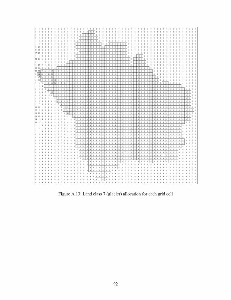
92
0 0 0 0 0 0 0 0 0 0 0 0 0 0 0 0 0 0 0 0 0 0 0 0 0 0 0 0 0 0 0 0 0 0 0 0 0 0 0 0 0 0 0 0 0 0 0 0 0 0 0
0 0 0 0 0 0 0 0 0 0 0 0 0 0 0 0 0 0 0 0 0 0 0 0 0 0 0 0 0 0 0 0 0 0 0 0 0 0 0 0 0 0 0 0 0 0 0 0 0 0 0
0 0 0 0 0 0 0 0 0 0 0 0 0 0 0 0 0 0 0 0 0 0 0 0 0 0 0 0 0 0 0 0 0 0 0 0 0 0 0 0 0 0 0 0 0 0 0 0 0 0 0
0 0 0 0 0 0 0 0 0 0 0 0 0 0 0 0 0 0 0 0 0 0 0 0 0 0 0 0 0 0 0 0 0 0 0 0 0 0 0 0 0 0 0 0 0 0 0 0 0 0 0
1 0 0 0 0 0 0 0 0 0 0 0 0 0 0 0 0 0 0 0 0 0 0 0 0 0 0 0 0 0 0 0 0 0 0 0 0 0 0 0 0 0 0 0 0 0 0 0 0 0 0
4 8 0 0 0 0 0 0 0 0 0 0 0 0 0 0 0 0 0 0 0 0 0 0 0 0 0 0 0 0 0 0 0 0 0 0 0 0 0 0 0 0 0 0 0 0 0 0 0 0 0
6 24 0 0 0 0 0 0 0 0 0 0 0 0 0 0 0 0 0 0 0 0 0 0 0 0 0 0 0 0 0 0 0 0 0 0 0 0 0 0 0 0 0 0 0 0 0 0 0 0 0
31 15 3 0 0 0 0 0 0 0 0 0 0 0 0 0 0 0 0 0 0 0 0 0 0 0 0 0 0 0 0 0 0 0 0 0 0 0 0 0 0 0 0 0 0 0 0 0 0 0 0
17 23 2 1 0 0 0 0 0 0 0 0 0 0 0 0 0 0 0 0 0 0 0 0 0 0 0 0 0 0 0 0 0 0 0 0 0 0 0 0 0 0 0 0 0 0 0 0 0 0 0
9 3 0 0 0 0 0 0 0 0 0 0 0 0 0 0 0 0 0 0 0 0 0 0 0 0 0 0 0 0 0 0 0 0 0 0 0 0 0 0 0 0 0 0 0 0 0 0 0 0 0
24 26 6 0 0 0 0 0 0 0 0 0 0 0 0 0 0 0 0 0 0 0 0 0 0 0 0 0 0 0 0 0 0 0 0 0 0 0 0 0 0 0 0 0 0 0 0 0 0 0 0
6 1 1 1 1 0 0 0 0 0 0 0 0 0 0 0 0 0 0 0 0 0 0 0 0 0 0 0 0 0 0 0 0 0 0 0 0 0 0 0 0 0 0 0 0 0 0 0 0 0 0
5 29 19 13 20 0 3 1 0 0 0 0 0 0 0 0 0 0 0 0 0 0 0 0 0 0 0 0 0 0 0 0 0 0 0 0 0 0 0 0 0 0 0 0 0 0 0 0 0 0 0
10 11 18 45 26 0 2 0 0 0 0 0 0 0 0 0 0 0 0 0 0 0 0 0 0 0 0 0 0 0 0 0 0 0 0 0 0 0 0 0 0 0 0 0 0 0 0 0 0 0 0
25 32 19 26 19 15 3 4 0 0 0 0 0 0 0 0 0 0 0 0 0 0 0 0 0 0 0 0 0 0 0 0 0 0 0 0 0 0 0 0 0 0 0 0 0 0 0 0 0 0 0
2 32 35 10 26 30 0 3 0 0 0 0 0 0 0 0 0 0 0 0 0 0 0 0 0 0 0 0 0 0 0 0 0 0 0 0 0 0 0 0 0 0 0 0 0 0 0 0 0 0 0
3 47 34 9 5 20 6 0 0 0 0 0 0 0 0 0 0 0 0 0 0 0 0 0 0 0 0 0 0 0 0 0 0 0 0 0 0 0 0 0 0 0 0 0 0 0 0 0 0 0 0
6 11 9 1 3 18 12 1 0 0 0 0 0 0 0 0 0 0 0 0 0 0 0 0 0 0 0 0 0 0 0 0 0 0 0 0 0 0 0 0 0 0 0 0 0 0 0 0 0 0 0
7 0 14 13 0 11 21 0 2 2 1 0 0 0 0 0 0 0 0 0 0 0 0 0 0 0 0 0 0 0 0 0 0 0 0 0 0 0 0 0 0 0 0 0 0 0 0 0 0 0 0
1 5 4 21 17 4 2 0 0 1 0 0 0 0 0 0 0 0 0 0 0 0 0 0 0 0 0 0 0 0 0 0 0 0 0 0 0 0 0 0 0 0 0 0 0 0 0 0 0 0 0
0 0 10 9 6 5 0 0 0 0 0 0 0 0 0 0 0 0 0 0 0 0 0 0 0 0 0 0 0 0 0 0 0 0 0 0 0 0 0 0 0 0 0 0 0 0 0 0 1 0 0
0 0 0 7 3 10 0 0 0 0 0 0 0 0 0 0 0 0 0 0 0 0 0 0 0 0 0 0 0 0 0 0 0 0 0 0 0 0 0 0 0 0 0 0 0 0 0 0 0 0 0
0 0 0 1 12 0 0 0 0 0 0 0 0 0 0 0 0 0 0 0 0 0 0 0 0 0 0 0 0 0 0 0 0 0 0 0 0 0 0 0 0 0 0 0 0 0 0 0 0 0 0
4 0 0 0 1 1 0 3 6 0 1 0 0 0 0 0 0 0 0 0 0 0 0 0 0 0 0 0 0 0 0 0 0 0 0 0 0 0 0 0 0 0 0 0 0 0 0 0 0 0 0
8 0 0 0 0 0 2 27 2 0 2 1 0 0 0 0 0 0 0 0 0 0 0 0 0 0 0 0 0 0 0 0 0 0 0 0 0 0 0 0 0 0 0 0 0 0 0 0 0 0 0
5 7 0 0 0 0 0 5 4 1 2 0 0 0 0 0 0 0 0 0 0 0 0 0 0 0 0 0 0 0 0 0 0 0 0 0 0 0 0 0 0 0 0 0 0 0 0 0 0 0 0
13 11 1 0 0 0 0 0 7 18 2 1 3 0 0 0 0 0 0 0 0 0 0 0 0 0 0 0 0 0 0 0 0 0 0 0 0 0 0 0 0 0 0 0 0 0 0 0 0 0 0
12 5 0 0 0 0 0 0 2 9 4 0 3 3 0 0 0 0 0 0 0 0 0 0 0 0 0 0 0 0 0 0 0 0 0 0 0 0 0 0 0 0 0 0 0 0 0 0 0 0 0
15 23 10 0 0 0 0 0 0 1 18 0 0 0 0 0 0 0 0 0 0 0 0 0 0 0 0 0 0 0 0 0 0 0 0 0 0 0 0 0 0 0 0 0 0 0 0 0 0 0 0
10 11 0 0 0 0 0 0 0 2 8 2 0 0 0 0 0 0 0 0 0 0 0 0 0 0 0 0 0 0 0 0 0 0 0 0 0 0 0 0 0 0 0 0 0 0 0 0 0 0 0
14 2 4 0 0 0 0 0 0 0 1 0 0 0 0 0 0 0 0 0 0 0 0 0 0 0 0 0 0 0 0 0 0 0 0 0 0 0 0 0 0 0 0 0 0 0 0 0 0 0 0
13 2 1 1 0 0 0 0 0 0 0 0 0 0 0 0 0 0 0 0 0 0 0 0 0 0 0 0 0 0 0 0 0 0 0 0 0 0 0 0 0 0 0 0 0 0 0 0 0 0 0
5 1 0 0 0 0 0 0 0 0 0 0 0 0 0 0 0 0 0 0 0 0 0 0 0 0 0 0 0 0 0 0 0 0 0 0 0 0 0 0 0 0 0 0 0 0 0 0 0 0 0
1 9 1 0 0 0 0 0 0 0 2 0 0 0 0 0 0 0 0 0 0 0 0 0 0 0 0 0 0 0 0 0 0 0 0 0 0 0 0 0 0 0 0 0 0 0 0 0 0 0 0
3 1 0 0 0 0 0 0 0 0 0 0 0 1 0 0 0 0 0 0 0 0 0 0 0 0 0 0 0 0 0 0 0 0 0 0 0 0 0 0 0 0 0 0 0 0 0 0 0 0 0
0 0 0 0 0 0 0 0 0 0 1 0 0 0 0 0 0 0 0 0 0 0 0 0 0 0 0 0 0 0 0 0 0 0 0 0 0 0 0 0 0 0 0 0 0 0 0 0 0 0 0
0 0 0 0 0 0 0 0 0 0 0 0 0 0 0 0 0 0 0 0 0 0 0 0 0 0 0 0 0 0 0 0 0 0 0 0 0 0 0 0 0 0 0 0 0 0 0 0 0 0 0
0 0 0 0 0 0 0 0 0 0 0 0 0 0 0 0 0 0 0 0 0 0 0 0 0 0 0 0 0 0 0 0 0 0 0 0 0 0 0 0 0 0 0 0 0 0 0 0 0 0 0
0 0 0 0 0 0 0 0 0 0 0 0 0 0 0 0 0 0 0 0 0 0 0 0 0 0 0 0 0 0 0 0 0 0 0 0 0 0 0 0 0 0 0 0 0 0 0 0 0 0 0
0 0 0 0 0 0 0 0 0 0 0 0 0 0 1 0 0 0 0 0 0 0 0 0 0 0 0 0 0 0 0 0 0 0 0 0 0 0 0 0 0 0 0 0 0 0 0 0 0 0 0
0 0 0 0 0 0 0 0 0 0 0 0 0 0 0 0 0 0 0 0 0 0 0 0 0 0 0 0 0 0 0 0 0 0 0 0 0 0 0 0 0 0 0 0 0 0 0 0 0 0 0
0 0 0 0 0 0 0 0 0 0 0 0 0 0 0 0 0 0 0 0 0 0 0 0 0 0 0 0 0 0 0 0 0 0 0 0 0 0 0 0 0 0 0 0 0 0 0 0 0 0 0
0 0 0 0 0 0 0 0 0 0 0 0 0 0 0 0 0 0 0 0 0 0 0 0 0 0 0 0 0 0 0 0 0 0 0 0 0 0 0 0 1 0 0 0 0 0 0 0 0 0 0
0 0 0 0 0 0 0 0 0 0 0 0 0 0 0 0 0 0 1 0 0 0 0 0 0 0 0 0 0 0 0 0 0 0 0 0 0 0 0 0 0 0 0 0 0 0 0 0 0 0 0
0 0 0 0 0 0 0 0 0 0 0 0 0 0 0 0 0 0 0 0 0 0 0 0 0 0 0 0 0 0 0 0 0 0 0 0 0 0 0 0 0 0 0 0 0 0 0 0 0 0 0
0 0 0 0 0 0 0 0 0 0 0 0 0 0 0 0 0 0 0 0 0 0 0 0 0 0 0 0 0 0 0 0 0 0 0 0 0 0 0 0 0 0 0 0 0 0 0 0 0 0 0
0 0 0 0 0 0 0 0 0 0 0 0 0 0 0 0 1 0 0 1 0 0 0 0 0 0 0 0 0 0 0 0 0 0 0 0 0 0 0 0 0 0 0 0 0 0 0 0 0 0 0
0 0 0 0 0 0 0 0 0 0 0 0 0 0 0 0 0 0 0 1 0 0 0 0 0 0 0 0 0 0 0 0 0 0 0 0 0 0 0 0 0 0 0 0 0 0 0 0 0 0 0
0 0 0 0 0 0 0 0 0 0 0 0 0 0 0 0 0 0 0 0 0 0 0 0 0 0 0 0 0 0 0 0 0 0 0 0 0 0 0 0 0 0 0 0 0 0 0 0 0 0 0
0 0 0 0 0 0 0 0 0 0 0 0 0 0 0 0 0 0 0 0 0 0 0 0 0 0 0 0 0 0 0 0 0 0 0 0 0 0 0 0 0 0 0 0 0 0 0 0 0 0 0
0 0 0 0 0 0 0 0 0 0 0 0 0 0 0 0 0 0 0 0 1 0 0 0 0 0 0 0 0 0 0 0 0 0 0 0 0 0 0 0 0 0 0 0 0 0 0 0 0 0 0
0 0 0 0 0 0 0 0 0 0 0 0 0 0 0 0 0 0 0 0 0 0 0 0 0 0 0 0 0 0 0 0 0 0 0 0 0 0 0 0 0 0 0 0 0 0 0 0 0 0 0
Figure A.13: Land class 7 (glacier) allocation for each grid cell

93
0 0 0 0 0 0 0 0 0 9 0 0 0 0 7 2 0 0 0 48 2 0 0 0 0 1 16 0 0 0 0 0 0 0 0 0 0 0 0 0 0 0 0 0 0 0 0 0 0 0 0
1 0 0 0 0 0 0 0 4 28 36 0 0 0 8 15 0 0 0 22 13 0 0 0 0 0 16 0 0 0 0 0 0 0 0 0 0 0 0 0 0 0 0 0 0 0 0 0 0 0 0
0 0 0 0 0 0 0 0 0 0 1 0 0 0 0 0 0 0 0 0 0 0 0 0 0 0 0 0 0 0 0 0 5 1 0 0 0 0 0 0 0 0 0 0 0 0 0 0 0 0 0
0 1 1 0 0 0 0 0 0 0 0 0 0 0 0 0 0 0 0 0 0 0 0 0 0 0 0 0 0 0 0 0 11 2 0 0 0 0 0 0 0 0 0 0 0 0 0 0 6 6 0
6 3 2 0 0 0 0 0 0 0 0 0 0 0 0 0 0 0 0 0 0 0 0 0 0 9 16 0 0 0 0 0 0 0 0 0 0 0 0 0 0 0 0 0 0 0 0 0 44 31 0
1 0 1 4 0 0 0 0 0 0 0 0 0 0 0 0 0 0 0 17 0 0 0 0 0 0 8 0 0 0 0 0 0 0 0 0 0 0 0 0 0 0 0 0 0 0 0 0 4 13 2
1 0 0 1 0 0 0 0 0 0 0 0 0 0 0 0 0 0 0 31 11 0 0 0 0 0 2 8 0 0 0 0 0 0 0 0 0 0 0 0 0 0 0 0 0 0 0 0 0 0 0
0 0 4 0 0 0 0 0 0 0 0 0 0 0 0 0 0 0 9 4 7 0 0 0 0 0 30 56 3 0 0 0 0 0 0 0 0 0 0 0 0 0 0 0 0 0 0 0 0 0 0
1 0 0 5 1 0 0 0 0 0 0 0 0 0 0 0 0 0 28 10 0 0 0 0 0 0 0 0 0 0 0 0 0 0 0 0 0 0 0 0 0 0 0 0 0 0 0 0 0 0 0
7 2 4 8 4 5 0 0 0 0 0 0 0 0 0 0 0 0 0 0 0 0 0 0 0 0 0 0 0 0 0 0 0 0 0 0 0 0 0 0 0 0 0 0 0 0 0 0 0 0 0
1 1 1 0 1 2 1 0 0 0 0 0 0 0 0 0 0 0 0 0 0 0 0 0 0 0 0 0 0 4 21 0 0 0 0 0 0 0 0 0 0 0 0 13 1 0 0 0 0 0 0
3 10 5 3 1 0 0 0 0 0 0 0 0 0 0 0 0 22 15 0 0 0 0 0 0 0 0 0 0 0 17 0 11 4 0 0 0 0 0 0 0 0 0 23 3 0 0 0 0 0 0
8 0 0 3 0 0 1 4 0 0 0 0 0 0 0 0 0 7 0 0 0 0 0 0 0 0 0 0 0 13 22 0 8 61 2 0 0 0 0 0 0 0 0 0 0 0 0 0 0 0 0
2 7 0 1 1 7 10 2 8 0 0 0 0 0 0 0 0 0 0 0 0 0 0 0 0 0 0 0 0 0 0 0 0 61 1 0 0 2 0 0 0 0 0 0 0 0 0 0 0 0 0
0 2 1 2 2 0 0 0 0 1 0 0 0 0 0 0 0 0 0 0 0 0 0 0 0 0 0 0 0 0 8 11 0 1 0 0 0 5 9 0 0 0 0 0 12 0 0 0 0 0 0
0 1 1 0 0 2 6 6 0 0 0 0 0 0 0 0 0 0 0 0 0 0 0 0 0 0 0 0 0 0 0 0 8 13 0 0 0 0 0 0 0 0 0 0 0 0 0 0 0 0 0
0 7 0 9 0 8 0 1 3 2 0 0 0 0 0 0 0 0 0 0 0 0 0 0 0 0 0 0 0 0 0 0 0 3 0 0 0 0 0 0 0 0 0 0 0 0 0 0 0 0 0
0 1 1 10 0 1 3 0 0 0 0 0 0 0 0 0 0 0 0 0 0 0 0 0 0 0 0 0 0 0 0 0 0 0 0 0 0 0 0 0 0 0 0 0 0 0 0 0 0 0 0
1 3 0 10 2 0 1 0 0 2 4 0 0 0 0 0 0 0 0 0 0 0 0 0 0 0 0 0 0 0 0 0 0 2 3 0 0 0 0 0 0 0 0 0 0 0 0 0 0 0 0
0 8 2 5 8 2 0 0 3 7 6 0 0 0 0 0 0 0 0 0 0 0 0 0 0 0 0 0 0 0 0 0 0 0 7 0 0 0 0 0 0 0 0 0 0 0 0 0 0 0 0
0 0 0 1 1 5 0 0 15 28 17 0 0 0 0 0 0 0 0 0 0 0 0 0 0 0 0 0 0 0 0 0 0 0 0 0 0 0 0 0 0 0 0 0 0 0 0 0 0 0 0
0 0 0 0 0 7 0 1 10 1 0 1 0 0 0 0 0 0 0 0 0 0 0 0 0 0 0 0 0 0 0 0 0 0 0 0 0 0 0 0 0 0 0 0 0 0 0 0 0 0 0
0 0 0 0 0 0 3 0 3 2 2 0 0 0 0 0 0 0 0 0 0 0 0 0 0 0 0 0 3 0 0 0 0 0 0 0 0 0 0 0 0 0 0 0 0 0 0 0 6 4 0
2 0 4 0 0 1 0 0 2 18 1 1 0 0 0 0 0 0 0 0 0 0 0 14 0 0 0 0 8 0 0 0 0 0 0 0 0 0 0 0 0 0 0 0 0 0 0 0 0 0 0
0 1 8 0 1 0 0 2 1 21 0 0 1 0 0 0 0 0 0 0 0 0 0 0 0 0 0 0 0 0 0 0 0 0 0 0 0 0 0 0 0 0 0 0 0 0 0 0 0 0 0
1 0 0 0 2 0 4 1 3 0 0 0 0 0 0 0 0 0 0 0 0 0 0 0 0 0 0 0 0 0 0 0 0 0 0 0 0 0 0 0 0 0 0 0 0 0 0 0 0 0 0
2 4 0 0 0 0 0 1 0 0 3 1 0 0 0 0 0 0 0 0 0 0 0 0 0 0 0 0 0 0 0 0 0 0 0 0 0 0 0 0 0 0 0 0 0 0 0 0 0 0 0
1 0 1 2 0 1 0 1 0 1 22 1 0 5 0 0 0 0 0 0 0 0 0 0 0 0 0 0 0 0 0 0 0 0 0 0 0 0 0 0 0 0 0 0 0 0 0 0 0 0 0
11 4 0 0 10 0 0 0 0 0 0 6 0 0 0 0 0 0 0 0 14 8 0 0 0 0 9 0 0 0 0 0 0 0 0 0 0 13 0 0 0 0 0 0 0 0 0 0 0 0 0
2 0 0 0 1 3 1 0 0 1 3 1 0 0 0 0 0 0 0 0 0 1 0 0 0 0 29 0 0 0 0 0 0 24 0 0 0 14 0 0 0 0 0 0 0 0 0 0 0 0 0
2 0 0 0 0 9 0 0 0 2 0 0 0 0 0 0 0 0 0 0 0 0 0 0 0 0 8 5 0 0 0 0 0 55 0 0 0 0 0 0 0 0 0 0 0 0 0 0 0 0 0
8 0 0 0 0 23 0 0 0 1 0 0 3 1 0 0 0 0 0 0 0 0 0 0 0 0 0 0 0 0 0 0 0 6 0 0 0 0 0 0 0 0 0 0 0 0 0 0 0 0 0
0 1 0 0 0 1 0 1 0 1 2 0 17 0 1 0 0 0 0 0 0 0 0 0 0 0 14 16 6 0 0 0 0 0 0 0 0 0 0 0 0 0 0 0 0 0 0 0 0 0 0
0 0 0 1 0 0 0 0 0 0 1 0 2 0 0 0 0 0 0 0 0 0 0 0 0 0 0 0 0 0 0 0 0 0 0 0 0 0 0 0 0 0 0 0 0 0 41 38 24 7 0
0 0 3 3 0 0 0 0 0 0 0 1 0 1 3 0 0 0 0 0 0 0 0 0 0 0 0 0 0 0 0 0 0 0 0 0 0 0 0 0 0 0 0 0 0 0 1 0 0 5 0
0 0 3 0 0 0 0 0 0 0 0 0 1 3 0 0 0 0 0 0 0 0 0 0 0 17 1 0 0 0 0 0 0 0 0 0 0 0 0 0 0 0 0 0 0 0 0 0 0 0 0
0 0 2 0 0 0 0 0 0 0 0 0 1 0 0 0 0 0 0 0 0 0 0 0 0 0 0 0 0 0 0 0 0 0 0 0 0 0 0 0 0 0 0 0 0 0 0 0 0 0 0
0 0 2 0 0 0 0 0 0 0 0 0 5 0 0 0 0 0 0 0 0 0 0 0 0 0 0 0 0 0 0 0 10 0 0 0 0 0 0 0 0 0 0 0 0 0 0 0 0 0 0
0 0 0 0 0 0 0 0 0 0 0 0 0 0 0 0 0 0 0 0 0 0 0 0 0 0 0 0 0 0 0 0 8 0 0 0 0 0 0 0 0 0 0 0 0 0 0 0 0 0 0
0 0 0 0 0 0 0 0 0 0 0 0 0 0 0 0 0 0 0 0 0 0 0 0 0 0 0 0 0 0 0 0 0 0 0 0 0 0 0 0 0 0 0 0 0 0 0 0 0 0 0
0 0 0 0 0 0 0 0 0 0 0 0 0 0 0 0 0 0 0 0 0 0 0 0 0 0 0 0 0 0 0 0 0 0 0 0 0 0 0 0 0 0 0 0 0 0 0 0 0 0 3
0 0 0 0 0 0 0 0 0 0 0 0 0 0 0 0 0 0 0 0 0 0 0 0 3 0 0 2 13 2 0 0 0 0 0 0 0 0 0 4 24 0 0 0 0 0 0 0 0 0 0
0 0 0 0 0 0 0 0 0 1 0 0 0 0 0 0 0 0 0 0 0 0 0 12 24 0 0 0 3 6 0 0 0 0 0 0 0 0 0 3 43 0 0 0 0 0 0 0 0 0 0
0 0 0 0 0 0 0 0 0 5 0 0 0 0 0 0 0 1 0 0 0 0 0 1 0 0 0 0 0 0 0 0 0 0 0 0 0 0 0 10 18 0 0 0 0 0 0 0 0 0 0
26 19 12 5 1 0 0 0 0 4 0 0 0 0 0 0 0 0 0 0 0 0 0 0 0 0 0 0 0 0 0 0 0 0 0 0 0 0 0 0 0 0 0 0 0 0 0 0 0 0 0
100 100 100 100 98 93 87 82 76 70 64 58 53 49 43 40 34 9 5 7 0 0 0 0 0 1 1 5 0 0 0 0 0 0 0 0 0 0 0 0 0 0 0 0 0 0 0 0 0 0 0
100 100 100 100 100 100 100 100 100 100 100 100 100 100 100 100 29 3 4 7 3 0 0 1 0 3 8 10 10 11 80 90 88 87 86 85 86 84 84 83 82 85 85 86 86 87 87 88 90 92 93
100 100 100 100 100 100 100 100 100 100 100 100 100 100 100 100 23 0 0 9 5 2 1 3 1 0 0 0 0 0 85 100 100 100 100 100 100 100 100 100 100 100 100 100 100 100 100 100 100 100 100
100 100 100 100 100 100 100 100 100 100 100 100 100 100 100 100 16 0 1 0 5 3 2 1 0 0 0 0 0 38 100 100 100 100 100 100 100 100 100 100 100 100 100 100 100 100 100 100 100 100 100
100 100 100 100 100 100 100 100 100 100 100 100 100 100 100 100 7 1 0 1 4 5 0 2 0 0 0 0 0 53 100 100 100 100 100 100 100 100 100 100 100 100 100 100 100 100 100 100 100 100 100
100 100 100 100 100 100 100 100 100 100 100 100 100 100 100 100 52 0 10 1 3 0 3 0 1 0 0 0 11 89 100 100 100 100 100 100 100 100 100 100 100 100 100 100 100 100 100 100 100 100 100
100 100 100 100 100 100 100 100 100 100 100 100 100 100 100 100 96 11 0 0 0 3 2 1 3 0 0 27 91 100 100 100 100 100 100 100 100 100 100 100 100 100 100 100 100 100 100 100 100 100 100
Figure A.14: Land class 8 (water) allocation for each grid cell

94
0 0 0 0 0 0 0 0 0 0 0 0 0 0 0 0 0 0 0 0 0 0 0 0 0 0 0 0 0 0 0 0 0 0 0 0 0 0 0 0 0 0 0 0 0 0 0 0 0 0 0
0 0 0 0 0 0 0 0 0 0 0 0 0 0 0 0 0 0 0 0 0 0 0 0 2 0 0 11 0 0 0 0 0 0 0 0 0 0 0 0 0 0 0 0 0 0 0 0 0 0 0
0 0 0 0 0 0 0 0 0 0 0 0 0 0 0 0 0 0 0 0 0 0 0 0 0 0 0 0 0 0 0 0 0 0 0 0 0 0 0 0 0 0 0 0 0 0 0 0 0 0 0
0 0 0 0 0 0 0 0 0 0 0 0 0 0 0 0 0 0 0 0 0 0 0 0 0 0 0 0 0 0 0 0 0 0 0 0 0 0 0 0 0 0 0 0 0 0 0 0 0 0 0
0 0 0 0 0 0 0 0 0 0 0 0 0 0 0 0 0 0 0 0 0 0 0 0 0 0 0 0 0 0 0 0 0 0 0 0 0 0 0 0 0 0 0 0 0 0 0 0 0 0 0
0 0 0 0 0 0 0 0 0 0 0 0 0 0 0 0 0 0 0 0 0 0 0 0 0 0 0 0 0 0 0 0 0 0 0 0 0 0 0 0 0 0 0 0 0 0 0 0 0 0 0
0 0 0 0 0 0 0 0 0 0 0 0 0 0 0 0 0 0 0 0 0 0 0 0 0 0 0 0 0 0 0 0 0 0 0 0 0 0 0 0 0 0 0 0 0 0 0 0 0 0 0
0 0 0 0 0 0 0 0 0 0 0 0 0 0 0 0 0 0 0 0 0 0 0 0 0 0 0 0 0 0 0 0 0 0 0 0 0 0 0 0 0 0 0 0 0 0 0 0 0 0 0
0 0 0 0 0 0 0 0 0 0 0 0 0 0 0 0 0 0 0 0 0 0 0 0 0 0 0 0 0 0 0 0 0 0 0 0 0 0 0 0 0 0 0 0 0 0 0 0 0 0 0
0 0 0 0 0 0 0 0 0 0 0 0 0 0 0 0 0 0 0 0 11 20 0 0 0 0 0 0 0 0 0 0 0 0 0 0 0 0 0 0 0 0 0 0 0 0 0 0 0 0 0
0 0 0 0 0 0 0 0 0 0 0 0 0 0 0 0 0 0 0 0 0 0 0 0 0 0 0 0 0 0 0 0 0 0 0 0 0 0 0 0 0 0 0 0 0 0 0 0 0 0 0
0 0 0 0 0 0 0 0 0 0 0 0 0 0 0 0 0 0 0 0 0 0 0 0 0 0 0 0 0 0 0 0 0 0 0 0 0 0 0 0 0 0 0 0 0 0 0 0 0 0 0
0 0 0 0 0 0 0 0 0 0 0 0 0 0 0 0 0 0 0 0 0 0 0 0 0 0 0 0 0 0 0 0 0 0 0 0 0 0 0 0 0 0 0 0 0 0 0 0 0 0 0
0 0 0 0 0 0 0 0 0 0 0 0 0 0 0 0 0 0 0 0 0 0 0 0 0 0 0 0 0 0 0 0 0 0 0 0 0 0 0 0 0 0 0 0 0 0 0 0 0 0 0
0 0 0 0 0 0 0 0 0 0 0 0 0 0 0 0 0 0 0 0 0 0 0 0 0 0 0 0 0 0 0 0 0 0 0 0 0 0 0 0 0 0 0 0 0 0 0 0 0 0 0
0 0 0 0 0 0 0 0 0 0 0 0 0 0 0 0 0 0 0 0 0 0 0 0 0 0 0 0 0 0 0 0 0 0 0 0 0 0 0 0 0 0 0 0 0 0 0 0 0 0 0
0 0 0 0 0 0 0 0 0 0 0 0 0 0 0 0 0 0 0 0 0 0 0 0 0 0 0 0 0 0 0 0 0 0 0 0 0 0 0 0 0 0 0 0 0 0 0 0 0 0 0
0 0 0 0 0 0 0 0 0 0 0 0 0 0 0 0 0 0 0 0 0 0 0 0 0 0 0 0 0 0 0 0 0 0 0 0 0 0 0 0 0 0 0 0 0 0 0 0 0 0 0
0 0 0 0 0 0 0 0 0 0 0 0 0 0 0 0 0 0 0 0 0 0 0 0 0 0 0 0 9 0 0 0 0 0 0 0 0 0 0 0 0 0 0 0 0 0 0 0 0 0 0
0 0 0 0 0 0 0 0 0 0 0 0 0 0 0 0 0 0 0 0 0 0 0 0 0 0 0 0 0 0 0 0 0 0 0 0 0 0 0 0 0 0 0 0 0 0 0 0 0 0 0
0 0 0 0 0 0 0 0 0 0 0 0 0 0 0 0 0 0 0 0 0 0 0 0 0 0 0 0 0 0 0 0 0 0 0 0 0 0 0 0 0 0 0 0 0 0 0 0 0 0 0
0 0 0 0 0 0 0 0 0 0 0 0 0 0 0 0 0 5 26 4 0 0 0 0 0 0 0 0 0 0 0 0 0 0 0 0 0 0 0 0 0 0 0 0 0 0 0 0 0 0 0
0 0 0 0 0 0 0 0 0 0 0 0 0 0 0 0 0 64 100 57 0 0 0 0 0 0 0 0 0 0 0 0 0 0 0 0 0 0 0 0 0 0 0 0 0 0 0 0 0 0 0
0 0 0 0 0 0 0 0 0 0 0 0 0 0 0 0 0 23 100 39 0 0 0 0 0 0 0 0 0 0 0 0 0 0 0 0 0 0 0 0 0 0 0 0 0 0 0 0 0 0 0
0 0 0 0 0 0 0 0 0 0 0 0 0 0 0 0 0 1 38 4 0 0 0 0 0 0 0 0 0 0 0 0 0 0 0 0 0 0 0 0 0 0 0 0 0 0 0 0 0 0 0
0 0 0 0 0 0 0 0 0 0 0 0 0 0 0 0 0 0 0 0 0 0 0 0 0 0 0 0 0 0 0 0 0 0 0 0 0 0 0 0 0 0 0 0 0 0 0 0 0 0 0
0 0 0 0 0 0 0 0 0 0 0 0 0 0 0 0 0 0 0 0 0 0 0 0 0 0 0 0 0 0 0 0 0 0 0 0 0 0 0 0 0 0 0 0 0 0 0 0 0 0 0
0 0 0 0 0 0 0 0 0 0 0 0 0 0 0 0 0 0 0 0 0 0 0 0 0 0 0 0 0 0 0 0 0 0 0 0 0 0 0 0 0 0 0 0 0 0 0 0 0 0 0
0 0 0 0 0 0 0 0 0 0 0 0 0 0 0 0 0 0 0 0 0 0 0 0 0 0 0 0 0 0 0 0 0 0 0 0 0 0 0 0 0 0 0 0 0 0 0 0 0 0 0
0 0 0 0 0 0 0 0 0 0 0 0 0 0 0 0 0 0 0 0 0 0 0 0 0 0 0 0 0 0 0 0 0 0 0 0 0 0 0 0 0 0 0 0 0 0 0 0 0 0 0
0 0 0 0 0 0 0 0 0 0 0 0 0 0 0 0 0 0 0 0 0 0 0 0 0 0 0 0 0 0 0 0 0 0 0 0 0 0 0 0 0 0 0 0 0 0 0 0 0 0 0
0 0 0 0 0 0 0 0 0 0 0 0 0 0 0 0 0 0 0 0 0 0 0 0 0 0 0 0 0 0 0 0 0 0 0 0 0 0 0 0 0 0 0 0 0 0 0 0 0 0 0
0 0 0 0 0 0 0 0 0 0 0 0 0 0 0 0 0 0 0 0 0 0 0 0 0 0 0 0 0 0 0 0 0 0 0 0 0 0 0 0 0 0 0 0 0 0 0 0 0 0 0
0 0 0 0 0 0 0 0 0 0 0 0 0 0 0 0 0 0 0 0 0 0 0 0 0 0 0 0 0 0 0 0 0 0 0 0 0 0 0 0 0 0 1 0 0 0 0 0 0 0 0
0 0 0 0 0 0 0 0 0 0 0 0 0 0 0 0 0 0 0 0 0 0 0 0 0 0 0 0 0 0 0 0 0 0 0 0 0 0 0 0 0 0 82 3 0 0 0 0 0 0 0
0 0 0 0 0 0 0 0 0 0 0 0 0 0 0 0 0 0 0 0 0 0 0 0 0 0 0 0 0 0 0 0 0 0 0 0 0 0 0 0 0 0 8 0 0 0 0 0 0 0 0
0 0 0 0 0 0 0 0 0 0 0 0 0 0 0 0 0 0 0 0 0 0 0 0 0 0 0 0 0 0 0 0 0 0 0 0 0 0 0 0 0 0 0 0 0 0 0 0 0 0 0
0 0 0 0 10 0 0 0 0 0 0 0 0 0 0 0 0 0 0 0 0 0 0 0 0 0 3 12 0 0 0 0 0 0 0 0 0 0 0 0 0 0 0 0 0 0 0 0 0 0 0
0 0 0 0 0 0 0 0 0 0 0 0 0 0 0 0 0 0 0 0 0 0 0 0 0 0 13 25 0 0 0 0 0 0 0 0 0 0 0 0 0 0 0 0 0 0 0 0 0 0 0
0 0 0 0 0 7 0 0 0 0 0 0 0 0 0 0 0 0 0 0 0 0 0 0 0 0 0 0 0 0 0 0 0 0 0 0 0 0 0 0 0 0 0 0 0 0 0 0 0 0 0
0 0 0 0 0 0 0 0 0 0 0 0 0 0 0 0 0 0 0 0 0 0 0 0 0 0 0 0 0 0 0 0 0 0 0 0 0 0 0 0 0 0 0 0 0 0 0 0 0 0 0
0 0 0 0 0 0 0 0 0 0 0 0 0 0 0 0 0 0 0 0 0 0 0 0 0 0 0 0 0 0 0 0 0 0 0 0 0 0 0 0 0 0 0 0 0 0 0 0 0 0 0
0 0 0 0 0 0 0 0 0 0 0 0 0 0 0 0 0 0 0 0 0 0 0 0 0 0 0 0 0 0 0 0 0 0 0 0 0 0 0 0 0 0 0 0 0 0 0 0 0 0 0
0 0 0 0 0 0 0 0 0 0 0 0 0 0 0 0 0 0 0 0 0 0 0 0 0 0 0 0 0 0 0 0 0 0 0 0 0 0 0 0 0 0 0 0 0 0 0 0 0 0 0
0 0 0 0 0 0 0 0 0 0 0 0 0 0 0 0 0 0 0 0 0 0 0 0 0 0 0 0 0 0 0 0 0 0 0 0 0 0 0 0 0 0 0 0 0 0 0 0 0 0 0
0 0 0 0 0 0 0 0 0 0 0 0 0 0 0 0 0 0 0 0 0 0 0 0 0 0 0 0 0 0 0 0 0 0 0 0 0 0 0 0 0 0 0 0 0 0 0 0 0 0 0
0 0 0 0 0 0 0 0 0 0 0 0 0 0 0 0 0 0 0 0 0 0 0 0 0 5 7 1 0 0 0 0 0 0 0 0 0 0 0 0 0 0 0 0 0 0 0 0 0 0 0
0 0 0 0 0 0 0 0 0 0 0 0 0 0 0 0 0 0 0 0 0 0 0 0 1 0 0 1 2 1 0 0 0 0 0 0 0 0 0 0 0 0 0 0 0 0 0 0 0 0 0
0 0 0 0 0 0 0 0 0 0 0 0 0 0 0 0 1 0 0 0 0 0 0 0 0 0 5 0 0 0 0 0 0 0 0 0 0 0 0 0 0 0 0 0 0 0 0 0 0 0 0
0 0 0 0 0 0 0 0 0 0 0 0 0 0 0 0 0 0 0 0 0 0 0 0 0 1 4 1 8 3 0 0 0 0 0 0 0 0 0 0 0 0 0 0 0 0 0 0 0 0 0
0 0 0 0 0 0 0 0 0 0 0 0 0 0 0 0 0 0 0 0 0 0 0 1 0 0 0 0 0 0 0 0 0 0 0 0 0 0 0 0 0 0 0 0 0 0 0 0 0 0 0
0 0 0 0 0 0 0 0 0 0 0 0 0 0 0 0 0 0 0 0 0 0 0 0 2 0 0 0 0 0 0 0 0 0 0 0 0 0 0 0 0 0 0 0 0 0 0 0 0 0 0
Figure A.15: Land class 9 (impervious) allocation for each grid cell

95
APPENDIX B
“MultiNash” Script This appendix contains the Visual Basin code for the multi-basin weighting script
“MultiNash”.
Private Sub MultiNash() Dim dbTemp As Double ‘Temp double Dim dbNash(1 To 30) As Double ‘Holds all 30 Nash daily values Dim dbFactor(1 To 30) As Double ‘Weighting factor for each stream gauge Dim dbSum As Double ‘Sum of streamflows from gauges in calc Dim dbSums(1 To 30) As Double ‘Sum (average) of each gauge’s streamflow Dim dbNewNash As Double ‘Holds weighted Nash daily value Open App.Path & "\nash_daily.csv" For Input As #1
Input #1, dbTemp ‘input blank line Input #1, dbTemp ‘input blank line Input #1, dbTemp ‘input blank line For I = 1 To 30 Input #1, dbNash(I) ‘input all 30 Nash daily values Input #1, dbTemp dbFactor(I) = 0 ‘set all factors to 0 Next I Close #1
‘ Set average streamflow for Basins used in Calibration ‘ Activate desired gauges, others are commented out ‘ dbSums(1) = 79106 ‘ dbSums(4) = 5662 dbSums(5) = 3229 ‘ dbSums(6) = 6753 ‘ dbSums(7) = 7568 dbSums(9) = 34972 dbSums(16) = 3533 ‘ dbSums(17) = 3301

96
‘ dbSums(19) = 7737 ‘ dbSums(20) = 13876 ‘ dbSums(21) = 1555 ‘ dbSums(22) = 4222 dbSums(23) = 9113 dbSums(25) = 3278 ‘ dbSums(26) = 12826 ‘ dbSums(27) = 2086 ‘ dbSums(28) = 1956 dbSum = 0 For I = 1 To 30 dbSum = dbSum + dbSums(I) ‘Add up streamflows from selected basins Next I For I = 1 To 30 dbFactor(I) = dbSums(I) / dbSum ‘Calculated weighting for each basin Next I dbNewNash = 0 For I = 1 To 30 dbNewNash = dbNewNash + dbNash(I) * dbFactor(I) ‘Calculates weighted Nash Next I Open App.Path & "\sum_nash.txt" For Output As #2 Print #2, dbNewNash ‘Prints weighted Nash Close #2 Unload MultiNash End Sub


