
arX
iv:1
206.
1736
v2 [
cond
-mat
.mes
-hal
l] 1
6 N
ov 2
012
TOPICAL REVIEW
Introduction to topological superconductivity and
Majorana fermions
Martin Leijnse and Karsten Flensberg
Center for Quantum Devices, Niels Bohr Institute, University of Copenhagen,
Universitetsparken 5, 2100 Copenhagen Ø, Denmark
E-mail: [email protected]
Abstract. This short review article provides a pedagogical introduction to the
rapidly growing research field of Majorana fermions in topological superconductors.
We first discuss in some detail the simplest ”toy model” in which Majoranas appear,
namely a one-dimensional tight-binding representation of a p-wave superconductor,
introduced more than ten years ago by Kitaev. We then give a general introduction
to the remarkable properties of Majorana fermions in condensed matter systems,
such as their intrinsically non-local nature and exotic exchange statistics, and
explain why these quasiparticles are suspected to be especially well suited for low-
decoherence quantum information processing. We also discuss the experimentally
promising (and perhaps already successfully realized) possibility of creating topological
superconductors using semiconductors with strong spin-orbit coupling, proximity-
coupled to standard s-wave superconductors and exposed to a magnetic field. The goal
is to provide an introduction to the subject for experimentalists or theorists who are
new to the field, focusing on the aspects which are most important for understanding
the basic physics. The text should be accessible for readers with a basic understanding
of quantum mechanics and second quantization, and does not require knowledge of
quantum field theory or topological states of matter.
1. Introduction
Topological superconductivity is an interesting state of matter, partly because it is
associated with quasiparticle excitations which are Majorana fermions (MFs). In
particle physics, MFs are (fermionic) particles which are their own anti-particles [1].
It is still unclear if there are elementary particles which are MFs, but they are likely to
exist as quasiparticle excitations in certain condensed matter systems, where a MF
is a quasiparticle which is its ”own hole”. The condensed matter version of MFs
have attracted massive theoretical interest, mainly because of their special exchange
statistics: They are non-abelian anyons [2], meaning that particle exchanges are non-
trivial operations which in general do not commute. This is unlike other known particle
types where an exchange operation merely has the effect of multiplying the wavefunction
with +1 (for bosons) or -1 (for fermions) or a general phase factor φ (for ”ordinary”

2
(abelian) anyons). Furthermore, a MF is in a sense half of a normal fermion, meaning
that a fermionc state is obtained as a superposition of two MFs.
It should be noted, however, that any fermion can be written as a combination
of two MFs, which basically corresponds to splitting the fermion into a real and an
imaginary part, each of which is a MF. Normally this is a purely mathematical operation
without physical consequences, since the two MFs are spatially localized close to each
other, overlap significantly, and cannot be addressed individually. When we talk about
MFs here, we mean that a fermionic state can be written as a superposition of two MFs
which are spatially separated (or prevented from overlapping in some other manner).
Such a highly delocalized fermionic state is protected from most types of decoherence,
since it cannot be changed by local perturbations affecting only one of its Majorana
constituents. The state can, however, be manipulated by physical exchange of MFs
because of their non-abelian statistics, which has lead to the idea of low-decoherence
topological quantum computation [3].
Being its own hole means that a MF must be an equal superposition of an electron
and a hole state. It is natural to search for such excitations in superconducting systems,
where the wavefunctions of Boguliubov quasiparticles have both an electron and a hole
component. The most common type of superconducting pairing is of so-called s-wave
symmetry, where Cooper pairs are formed of electrons with opposite spin projections
(forming a singlet). In second quantization language, the annihilation operator of a
Boguliubov quasiparticle in an s-wave superconductor has the form b = uc†↑ + vc↓,
where cσ annihilates a normal fermion with spin projection σ =↑, ↓ (we neglect for
simplicity to write out additional quantum numbers which are irrelevant here). Having
equal electron and hole components mean that MFs are instead associated with an
annihilation operator of the type γ = uc†σ+u∗cσ, which is hermitian and therefore equal
to the creation operator, γ = γ†. Note that, in contrast to the s-wave Boguliubov
quasiparticle operator, the fermion operators making up the MF have equal spin
projections. Such quasiparticles do not occur in most types of superconductors and
were instead first predicted to occur in the ν = 5/2 fractional quantum Hall state [4].
However, as we will discuss in more detail below, isolated MFs occur in general in
vortices and on edges of effectively spinless superconducting systems with triplet pairing
symmetry [5, 6, 7, 8, 9, 10, 11, 12, 13] (p-wave pairing symmetry in one dimension
(1D) and px ± ipy pairing symmetry in two dimensions (2D)). Triplet pairing has been
predicted for the ground state of the superconductor Sr2RuO4 [14], but is very sensitive
to disorder and has never been observed experimentally. However, the existence of
(spatially separated) MFs is a topological invariant [15] (hence the name topological
superconductors). As a result, they will exist in all systems with the same topological
properties as a p-wave or px±ipy-wave superconductor (we will come back to the precise
meaning of this later).
A few years ago, the search for MFs took a big step forward when Fu and Kane [16]
showed that px ± ipy-wave-like pairing may also occur for the surface states of a strong
topological insulator when brought into tunneling contact with an ordinary s-wave

3
superconductor (giving rise to proximity-induced superconductivity [17, 18, 19] in the
topological insulator). The necessary underlying physical ingredient is the strong spin-
orbit coupling of the topological insulator, giving rise to split bands with momentum-
dependent spin directions. In addition, by coupling the topological insulator also to a
magnetic insulator, the resulting induced Zeeman splitting lifts the Kramer’s degeneracy
and allows an effectively spinless regime to be reached. However, as was realized shortly
after the pioneering work of Kane and Fu, the strong spin-orbit coupling in certain two-
dimensional semiconductor quantum wells should also do the job [20, 21, 22]. Also here
superconductivity can be induced through the proximity effect and magnetism either
induced by a magnetic insulator [20] or provided by an external magnetic field [21].
Shortly thereafter, two works [23, 24] suggested a further simplification by instead
using 1D semiconducting wires. There have also been proposals to create MFs e.g.,
in vortices in doped topological insulators [25], on the interface between a ferromagnet
and a superconductor deposited on a two-dimensional topological insulator [26, 27, 28],
in cold atomic gases [29, 30], in carbon nanotubes [31, 32, 33], and using chains of
quantum dots [34], just to name a few.
During the last couple of years, a number of experimental groups have taken up
the challenge to create MFs. Very recently this quest may have seen success [35], and
several other groups have made observations which can be interpreted as signatures of
Majoranas [36, 37, 38, 39]. There is no doubt that these early findings will be scrutinized
in future experiments and time will tell which are genuine observations of Majorana
physics. In any case, once MFs have been conclusively produced and detected in the
lab, the truly exciting experimental work begins, to test their theoretically predicted
properties and to design setups for ever more advanced manipulation of the quantum
information they can encode.
In this short review article we give an introduction to the topic of topological
superconductivity and MFs, which is aimed at both experimental and theoretical
physicists without prior knowledge of the field. We explain the generic necessary
ingredients of topological superconductivity, as well as the basic properties of MFs,
and how they can be realized in standard semiconductors proximity-coupled to s-wave
superconductors. Two excellent review articles discussing the subject have appeared
recently [40, 41]. Therefore, we do not attempt to give an exhaustive review of the
subject, or to provide detailed derivations of all results, but instead focus on providing
physical insight into what we feel are the most important basic concepts. We also try
to convey the excitement over MFs by briefly discussing some of their exotic properties,
such as the non-abelian statistics and the resulting potential for topological quantum
computation. The text should be accessible for all readers with a basic knowledge of
quantum mechanics and the second quantization formalism.

4
2. Majorana fermions in p-wave superconductors
We start our discussion by introducing a simple Hamiltonian, describing a spinless p-
wave superconductor, which has eigenstates which are spatially isolated MFs. It is most
intuitive to start from a 1D tight-binding chain with p-wave superconducting pairing,
as first introduced by Kitaev [42], described by the Hamiltonian
Hchain = −µN∑
i=1
ni −N−1∑
i=1
(
tc†ici+1 +∆cici+1 + h.c.)
, (1)
where h.c. means hermitian conjugate, µ is the chemical potential, ci is the electron
annihilation operator for site i, and ni = c†ici is the associated number operator. The
superconducting gap, ∆, and hopping, t, are assumed to be the same for all sites. We
can then choose the superconducting phase φ to be zero, such that ∆ = |∆|. Note thattime-reversal symmetry is broken in Eq. (1) since we only consider one value for the spin
projection, i.e., effectively spinless electrons (we suppress the spin label). Furthermore,
the superconducting pairing is non-standard since it couples electrons with the same spin
(in contrast to standard s-wave pairing, which only couples electrons with opposite spin
projection). Note also that electrons on neighboring sites are paired: The sites cannot
be doubly occupied by the spinless electrons because of the Pauli exclusion principle.
We now want to rewrite Eq. (1) in terms of Majorana operators (we will see shortly
why this is useful). It was mentioned above that MFs are basically obtained by splitting
a fermion into its real and imaginary parts. Therefore we write
ci =1
2(γi,1 + iγi,2) , (2)
c†i =1
2(γi,1 − iγi,2) , (3)
where γi,j are Majorana operators living on site i. That they are indeed Majorana
operators is seen by inverting Eqs. (2)–(3), giving
γi,1 = c†i + ci, (4)
γi,2 = i(
c†i − ci)
, (5)
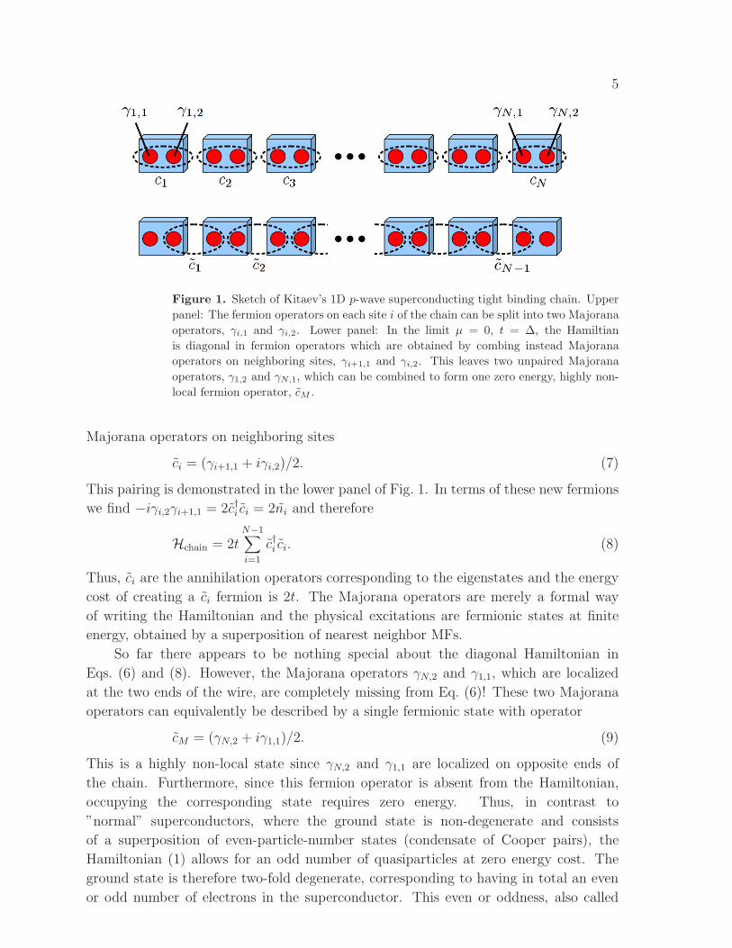
which are clearly hermitian and therefore Majorana operators. Figure 1 shows a sketch
of Kitaev’s chain and the upper panel indicates how the fermion operators on each site
are split into Majorana operators.
The Majorana physics is most easily understood when µ = 0, t = ∆, in which case
inserting Eqs. (2)–(3) into the Hamiltonian (1) results in
Hchain = −itN−1∑
i=1
γi,2γi+1,1. (6)
In fact, Eq. (6) is nothing but an alternative way of writing the diagonalized
Hamiltonian. To see this we go back to a fermionic representation by noting that,
analogous to Eqs. (2)–(3), where a fermion on site i was split into two Majorana
operators living on site i, we can construct new fermion operators, ci, by combining
5
Figure 1. Sketch of Kitaev’s 1D p-wave superconducting tight binding chain. Upper
panel: The fermion operators on each site i of the chain can be split into two Majorana
operators, γi,1 and γi,2. Lower panel: In the limit µ = 0, t = ∆, the Hamiltian
is diagonal in fermion operators which are obtained by combing instead Majorana
operators on neighboring sites, γi+1,1 and γi,2. This leaves two unpaired Majorana
operators, γ1,2 and γN,1, which can be combined to form one zero energy, highly non-
local fermion operator, cM .
Majorana operators on neighboring sites
ci = (γi+1,1 + iγi,2)/2. (7)
This pairing is demonstrated in the lower panel of Fig. 1. In terms of these new fermions
we find −iγi,2γi+1,1 = 2c†i ci = 2ni and therefore
Hchain = 2tN−1∑
i=1
c†i ci. (8)
Thus, ci are the annihilation operators corresponding to the eigenstates and the energy
cost of creating a ci fermion is 2t. The Majorana operators are merely a formal way
of writing the Hamiltonian and the physical excitations are fermionic states at finite
energy, obtained by a superposition of nearest neighbor MFs.
So far there appears to be nothing special about the diagonal Hamiltonian in
Eqs. (6) and (8). However, the Majorana operators γN,2 and γ1,1, which are localized
at the two ends of the wire, are completely missing from Eq. (6)! These two Majorana
operators can equivalently be described by a single fermionic state with operator
cM = (γN,2 + iγ1,1)/2. (9)
This is a highly non-local state since γN,2 and γ1,1 are localized on opposite ends of
the chain. Furthermore, since this fermion operator is absent from the Hamiltonian,
occupying the corresponding state requires zero energy. Thus, in contrast to
”normal” superconductors, where the ground state is non-degenerate and consists
of a superposition of even-particle-number states (condensate of Cooper pairs), the
Hamiltonian (1) allows for an odd number of quasiparticles at zero energy cost. The
ground state is therefore two-fold degenerate, corresponding to having in total an even
or odd number of electrons in the superconductor. This even or oddness, also called
6
parity, corresponds to the eigenvalue of the number operator of the zero-energy fermion,
nM = c†M cM = 0(1) for even (odd) parity.
The above argument was made for the very special case ∆ = t and µ = 0, but one
can show that the Majorana end states remain as long as the chemical potential lies
within the gap [42], |µ| < 2t. In the general case, however, the MFs are not completely
localized only at the two edge sites of the wire, but decay exponentially away from the
edges. The MFs remain at zero energy only if the wire is long enough that they do not
overlap.
The Hamiltonians for the continuum version of a p-wave superconductor in 1D and
2D are
Hpw1D =
∫
dx
[
Ψ†(x)
(
p2x2m
− µ
)
Ψ(x) + Ψ(x)|∆|eiφpxΨ(x) + h.c.
]
, (10)
Hpw2D =
∫
d2r
[
Ψ†(r)
(
p2
2m− µ
)
Ψ(r) + Ψ(r)|∆|eiφ (px ± ipy) Ψ(r) + h.c.
]
,
(11)
where Ψ†(r) is the real-space creation operator, p is the momentum, m is the effective
electron mass, and we have re-introduced the superconducting phase φ. As we saw
above, in the 1D case MFs appear at the edges of the wire. They will also appear
at transition points between topological and non-topological regions. For example, if
the chemical potential or the hopping amplitude varies along the wire and |µ| > 2t in
some segment, two additional MFs will appear at the transition points where the gap
closes [23].
Similarly, in a 2D px ± ipy-wave superconductor, MFs appear in vortices in the
superconducting pairing potential [6, 8, 10]. Alternatively, MFs can appear if the gap is
closed by variations in the chemical potential or electrostatic potential [11]. It is worth
noting that isolated MFs can appear even in a spinful px ± ipy-wave superconductor, in
so-called half-quantum vortices [8], where there is a vortex for only one direction of the
triplet (note that this also means a breaking of time-reversal symmetry).
If there are in total an odd number of gap closings, an additional MF will appear
somewhere in the system to guarantee that there is always an even number (exactly
where this additional MF appears depends on the details, see Ref. [40] for a detailed
discussion).
3. Properties of Majorana fermions
Before explaining how MFs can be realized in more realistic systems, we now discuss
in more detail some of their generic properties, which are independent of the specific
system in which they appear.

7
3.1. Representation in terms of fermionic operators
Let us assume that we have a system with 2N spatially well-separated MFs, γ1, . . . γ2N .
The number of MFs is necessarily even since one MF contains half the degrees of freedom
of a normal fermion. Similar to the case of Kitaev’s chain, the Majorana operators are
obtained by splitting a normal fermion fi in its real and imaginary parts (cf., Eq. (9))
fi = (γ2i−1 + iγ2i)/2. (12)
The inverse relation is then
γ2i−1 = f † + f, (13)
γ2i = i(f † − f). (14)
Obviously, the Majorana operators are hermitian, γj = γ†j . Using the fermionic
anti-commutation relations for the fi-fermions, it is easily verified that the Majorana
operators satisfy the anti-commutation relation
{γi, γj} = 2δij , (15)
which is somewhat reminiscent of normal fermions. There are, however, important
differences. From Eq. (15), we see that γ2i = 1. Thus, acting twice with a Majorana
operator, we get back the same state we started with. There is therefore no Pauli
principle for MFs (cf., c2 = (c†)2 = 0 for normal fermion operators c). In fact, we
cannot even speak of the occupancy of a Majorana mode. We can try to count the
occupancy by constructing a ”Majorana number operator”, nMFi = γ†i γi. However,
using hermiticity, γ†i = γi, together with γ2i = 1, we find nMF
i ≡ 1. Similarly, γiγ†i ≡ 1.
Thus, the Majorana mode is in a sense always empty and always filled and counting
does not make any sense.
It would still be very useful to use some sort of number states. These are instead
provided through the fi fermions as we already saw above in the example with Kitaev’s
chain. Since these are normal fermions, there are number states |n1, . . . , nN〉 which are
eigenstates of the fermionic number operators, ni = f †i fi, with eigenvalue ni = 0, 1 (by
Pauli exclusion principle). Note that the labelling of the γ’s, and thereby the pairing
into fermionic states, is arbitrary and merely represents a choice of basis for the number
states. However, if two MFs come close enough to overlap, it is natural to choose to
combine them into a fermion. To describe an overlap, t, between γ2i−1 and γ2i, the only
term one can introduce into the Hamiltonian isi
2tγ2i−1γ2i = t
(
ni −1
2
)
, (16)
which corresponds to a finite energy cost for occupying the corresponding fermionic state
(t > 0). If the MFs do not overlap, the groundstate is 2N -fold degenerate, corresponding
to each ni being equal to zero or one. The sum of all occupation numbers,∑N
i=1 ni, being
even or odd now reflects whether the total number of electrons in the superconductor is
even or odd (even or odd parity). To change the parity, electrons have to be physically
added to or removed from the superconductor.
8
The experimentally measurable quantities are the occupation numbers ni. Such
a measurement can be done by bringing two MFs close together and measuring the
energy of the corresponding state [43], which reveals the occupation through Eq. (16).
One could also use interferometry [44] or coupling to conventional superconducting
qubits [45]. Note that it does not make sense to talk about the ”state of a MF” since a
single MF contains only ”half a degree of freedom”. The only physical observables are
the fermionic occupation numbers.
3.2. Non-abelian statistics
It is a crucial ingredient for non-abelian statistics to have a degenerate groundstate,
which is separated from all excited states by a gap (ideally the induced superconducting
gap, but it could also be a smaller gap to for example finite-energy vortex- or edge
states). Then adiabatic operations, such as the slow exchange of quasiparticle positions,
can in principle bring the system from one groundstate to another. It is, of course,
not obvious that such a transformation indeed takes place, which will depend on the
details of the system. In the case of MFs in a px ± ipy superconductor, Ivanov [8]
provided a simple and elegant proof of the non-abelian statistics which we sketch here.
(The Supplementary Information of Ref. [46] provides a proof in the case of 1D wires,
where MFs can be moved using closely spaced electronic ”keyboard” gates and particle
exchange is made possible by connecting the 1D wires in T-junctions.)
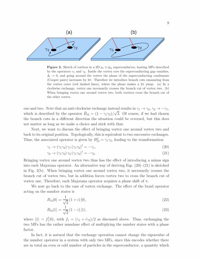
Imagine that we have two vortices in a two-dimensional topological superconductor,
hosting MFs described by the operators γ1 and γ2 at the vortex cores, see Fig. 2. Each
vortex is associated with a winding of 2π of the superconducting phase φ. We can
choose φ to be single-valued everywhere, except for at branch cuts (red dashed lines in
Fig. 2) emanating from each vortex, such that φ changes by 2π when crossing this line
(the direction of the branch cuts can be chosen arbitrarily). Vortices could perhaps be
moved using the tip of a scanning tunneling microscope, or by local magnetic gates. If
we now exchange vortices one and two in a clockwise manner as indicated in Fig. 2(a),
vortex 1 crosses a branch cut and acquires a 2π phase shift, while vortex 2 does not
acquire a phase. The superconducting phase is the phase of the Cooper pairs in the
condensate. The MF in vortex 1, which is made up from single (rather than products of
two) fermion operators, then acquires a phase of π upon crossing the branch cut. The
result of this exchange operation is thus
γ1 → − γ2, (17)
γ2 → + γ1. (18)
This transformation is described by γi → B12γiB†12, where the so-called braid operator
is given by
B12 =1√2(1 + γ1γ2) . (19)
This choice of operator is made unique by requiring that, in a system with more than two
vortices (and therefore MFs), all the others are unaffected by the exchange of vortices
9
Figure 2. Sketch of vortices in a 2D px ± ipy superconductor, hosting MFs described
by the operators γ1 and γ2. Inside the vortex core the superconducting gap vanishes,
∆ → 0, and going around the vortex the phase of the superconducting condensate
(Cooper pairs) increases by 2π. Therefore we introduce branch cuts emanating from
the vortex cores (red dashed lines), where the phase makes a 2π jump. (a) In a
clockwise exchange, vortex one necessarily crosses the branch cut of vortex two. (b)
When bringing vortex one around vortex two, both vortices cross the branch cut of
the other vortex.
one and two. Note that an anti-clockwise exchange instead results in γ1 → γ2, γ2 → −γ1,which is described by the operator B12 = (1 − γ1γ2)/
√2. Of course, if we had chosen
the branch cuts in a different direction the situation could be reversed, but this does
not matter as long as we make a choice and stick with that.
Next, we want to discuss the effect of bringing vortex one around vortex two and
back to its original position. Topologically, this is equivalent to two successive exchanges.
Thus, the associated operator is given by B212 = γ1γ2, leading to the transformation
γ1 → (γ1γ2) γ1 (γ1γ2)† = −γ1, (20)
γ2 → (γ1γ2) γ2 (γ1γ2)† = −γ2. (21)
Bringing vortex one around vortex two thus has the effect of introducing a minus sign
into each Majorana operator. An alternative way of deriving Eqs. (20)–(21) is sketched
in Fig. 2(b). When bringing vortex one around vortex two, it necessarily crosses the
branch cut of vortex two, but in addition forces vortex two to cross the branch cut of
vortex one. Therefore, each Majorana operator acquires a phase shift of π.
We now go back to the case of vortex exchange. The effect of the braid operator
acting on the number states is
B12|0〉 =1√2(1 + i) |0〉, (22)
B12|1〉 =1√2(1− i) |1〉, (23)
where |1〉 = f †1 |0〉, with f1 = (γ1 + iγ2)/2 as discussed above. Thus, exchanging the
two MFs has the rather mundane effect of multiplying the number states with a phase
factor.
In fact, it is natural that the exchange operation cannot change the eigenvalue of
the number operator in a system with only two MFs, since this encodes whether there
are in total an even or odd number of particles in the superconductor, a quantity which

10
is not changed by particle exchanges. To find non-trivial effects of exchange operations
we must consider a system with at least four MFs, described in terms of the fermionic
number states |n1n2〉. Let us now investigate the effect of exchanging neighboring MFs,
described by braid operators Bi,i+1. For simplicity we choose the branch cuts of all MFs
to be in the same direction and number the MFs based on their position orthogonal
to this direction, such that when exchanging MFs i and i + 1 in a clockwise manner,
vortex i crosses only the branch cut of vortex i + 1, and no other vortices cross any
branch cuts (crossing the same branch cut twice in different directions is equivalent to
not crossing any branch cuts at all). Note that MFs which are not neighbors can always
be exchanged through a sequence of neighbor exchanges. Consider now the effect of
braid operations on the number states
B12|00〉 =1√2(1 + i) |00〉, (24)
B23|00〉 =1√2(|00〉+ i|11〉) , (25)
B34|00〉 =1√2(1 + i) |00〉, (26)
with analogous results for the other number states. Note especially that B23, which
involves MFs from different fermions, produces a superposition state of different number
states. However, the total parity (n1 + n2 being even or odd) of each state in the
superposition must be the same.
With four MFs we can also demonstrate the non-abelian nature of braid operations
(with two MFs there is only one possible exchange operation). In general, two braid
operations commute whenever they do not involve any of the same MFs, [B12, B34] = 0.
This is easy to believe on physical grounds, as there is no reason that the exchange of
MFs three and four should care about whether MFs one and two have been exchanged.
However, whenever two exchanges involve some of the same MFs, the braid operators
do not commute
[Bi−1,i, Bi,i+1] = γi−1γi+1. (27)
Equation (27) expresses the non-abelian exchange statistics of MFs.
At this point the attentive reader might be slightly upset by a simple fact we have
neglected. Namely the question of what exactly qualifies as an exchange operation. If
we define an exchange operation as bringing one vortex exactly to the old position of
another vortex, and vice versa, there is no problem. But clearly this is not possible in
reality and certainly goes against the idea of robust topological quantum information
processing to be discussed below. (In networks of 1D wires it is somewhat easier to
find a satisfying definition of particle exchanges [46].) Mathematically, the exchange
process happens when the branch cut is crossed, but since this is arbitrarily defined,
it is not a good definition either. Physically, the solution to this problem is that there
is no measurable effect of the exchange process, unless it is followed by one of the two
MFs involved in the exchange being joined with a third MF to perform a measurement

11
Figure 3. Sketch demonstrating two equivalent sets of operations. In the upper panel,
MFs 2 and 3 are first exchanged (black arrows), then the nearest neighbor MFs are
brought together (magenta arrows) and the states of the corresponding fermions are
measured. In the lower panel, there is no exchange, but instead we directly measure
the fermions formed by pairing next-nearest neighboring MFs (1 + 3 and 2 + 4).
of the state of the fermion formed by this pair. This is demonstrated in Fig. 3. In the
upper panel, two neighboring MFs are first exchanged, which is followed by measuring
the fermionic states formed by pairing the nearest neighbor MFs. In the lower panel, on
the other hand, we do not exchange the MFs, but instead measure directly the fermionic
states formed by pairing next-nearest neighboring MFs. Both these operations give the
same result for the measurements of the fermionic states and are therefore equivalent.
Therefore, a ”computation” can be defined either as a set of exchanges, or by defining the
combinations of pairs that are being measured at the end, which removes the ambiguity
in defining an exchange process.
Another way of seeing this is to note that the result of a set of exchange operations
depends on the topology of the ”world lines” of the MFs (or other particles). The
world lines start when pairs of MFs are created from the vacuum, cross each other
when MFs are exchanged, and end when pairs of MFs are measured (fused). Only
sets of world lines which are topologically distinct can lead to different results, which
defines the so-called braid group, of which the MF exchange statistics is one possible
representation (fermions, bosons, and abelian anyons in general are the more trivial one-
dimensional representations). Non-abelian representations of the braid group exist only
in 2D (networks of 1D wires are also effectively 2D). Ref. [3] provides a more complete
mathematical discussion of these issues.

12
3.3. Majorana qubits and topological quantum computation
We saw above that parity conservation prevented braiding operations from changing the
state of a system with only two MFs. For this reason, the two-level system spanned
by the number operator n1 is not suitable to use as a qubit. To define a (topological)
Majorana qubit, we should therefore use four MFs, meaning two normal fermions [47],
and consider the case of fixed parity (even or odd) of the total number of fermions. Let
us consider the even parity subspace and define a qubit by |0〉 ≡ |00〉, |1〉 ≡ |11〉.In the basis {0, 1}, the Pauli matrices can be represented in terms of products of
Majorana operators
− iγ1γ2 = σz,−iγ3γ4 = σz (28)
−iγ2γ3 = σx, (29)
−iγ1γ3 = σy,−iγ2γ4 = σy (30)
which is seen by calculating the corresponding matrix elements. In the standard
representation with |0〉 and |1〉 being respectively the north and south poles of the
block sphere, we can then identify the different braids with single-qubit rotations
B12 = B34 = e−iπ
4σz , (31)
B23 = e−iπ
4σx , (32)
Thus, by braiding operations we can only perform single-qubit rotations by an angle
π/2.
When considering a multi-qubit setup, the most obvious choice is to define each
qubit in terms of four MFs [47]. However, it is not possible to construct a two-qubit
gate based on braiding operations which is able to create entanglement between two
such qubits. In addition, this choice does not use all the degrees of freedom offered
by the system. Even with conservation of the parity of the total number of fermions,
a system with 2N MFs has in principle enough degrees of freedom to store N − 1
qubits. Braiding-based gates acting on such ”overlapping” qubit systems have been
considered in Ref. [48]. No matter how the Majorana-based qubits are defined, braiding
operations can only explore a tiny fraction of the total Hilbert space and are insufficient
for universal quantum computation, which can, however, be achieved by including
also non-protected operations [43, 3], or by coupling Majorana qubits to other qubit
systems [45, 49, 50, 51, 52].
The advantage of Majorana-based qubits is that they keep the quantum information
encoded in delocalized fermionic states. Therefore, they are expected to be robust
against most sources of decoherence which do not couple simultaneously to more than
one Majorana mode, i.e., decoherence requires perturbations of the form γiγj, which
are suppressed when MFs i and j are spatially separated. An exception is processes
which change the total parity of the superconductor, e.g., by electrons tunneling into
a Majorana mode [53, 54, 55]. Such perturbations involve a single Majorana operator
(they are ∝ γi) and are not suppressed by keeping the MFs spatially separated. In fact,

13
this phenomena, known as quasiparticle poisoning [56, 57], is a well-known problem in
conventional (non-topological) superconducting qubits.
4. Proximity-induced superconductivity in spin-orbit semiconductors
Having seen how Majorana fermions appear in spinless p-wave (or px ± ipy-wave)
superconductors, we will now investigate how such exotic pairing can be engineered
using more readily available ingredients. We start, however, by considering the generic
effects of proximity-induced superconductivity.
The system we have in mind is a D-dimensional semiconductor, where D = 1 (wire)
or D = 2 (quantum well). Neglecting electron–electron interactions (or including them
in a mean-field manner), the system is described by the Hamiltonian
H0 =∑
σ=↑,↓
∫
dDr Ψ†σ(r)H0(r)Ψσ(r), (33)
where the first quantization single-particle Hamiltonian is given by
H0(r) =p2
2m− µ+ V (r) + α (E(r)× p) · σ +
1
2gµBB(r) · σ, (34)
where m is the effective electron mass, B is an applied magnetic field, µB is the Bohr
magneton, g is the Lande g factor, and σ is a vector of Pauli matrices. The spin-
orbit interaction with strength α has been written in the most general form in terms
of the electric field E felt by the valence electrons, and can involve both Rashba and
Dresselhaus terms.
If a good interface is made between a semiconductor and a superconductor,
electrons can tunnel between these two systems. The effect is that the electrons
in the semiconductor feels an effective ”proximity-induced” superconducting pairing
field [17, 18, 19]. The strength of this pairing field depends on the details of the
semiconductor and superconductor, as well as the interface. We do not attempt to
make an accurate microscopic model, but instead include the pairing effect in the
semiconductor by the phenomenological Hamiltonian
HS =∫
dDr dDr′ Ψ↓(r)∆(r, r′)Ψ↑(r′) + h.c., (35)
where ∆(r, r′) is the pairing potential. The pairing symmetry is inherited from the
superconductor, which we have here assumed to be s-wave, inducing singlet pairing
between spin-up and spin-down electrons.
When dealing with superconducting systems, it is standard practice to include both
the electrons and the holes explicitly by introducing so-called Nambu spinors
Ψ(r) =
Ψ↑(r)
Ψ↓(r)
Ψ†↓(r)
−Ψ†↑(r)
. (36)

14
Matrices acting on the Nambu spinors must have dimension 4×4 and we introduce Pauli
matrices τi, similar to σi, but acting in electron-hole space. Matrices such as τj ⊗ σithen have the appropriate 4× 4 structure. The total Hamiltonian can be written as
H = H0 +HS
=1
2
∫
dDr dDr′ Ψ†(r)[
H0(r)δ(r− r′) + ∆(r, r′)]
Ψ(r), (37)
where
H0(r) =
(
H0(r) 0σ0σ −σyH∗
0 (r)σy
)
, (38)
∆(r, r′) =
(
0σ ∆∗(r, r′)1σ∆(r, r′)1σ 0σ
)
. (39)
Note that these are 4× 4 matrices since H0(r) is a 2× 2 matrix and 0σ and 1σ denotes
respectively the zero and unit matrices in spin space. The term −σyH∗0 (r)σy in Eq. (38)
denotes the time-reversal of H0(r) and appears since holes are time-reversed electrons.
(Note, however, that we have not introduced any new physics with the matrices in
Eqs. (38)–(39), they are simply defined to give the correct total Hamiltonian, given by
Eq. (33) + Eq. (35).)
The quasiparticle excitations of a superconducting system are given by solving
the Bogoliubov-de Gennes equations for the eigenstates ψi(r) (which are also four-
component spinors)
H0(r)ψi(r) +∫
dDr′ ∆(r, r′)ψi(r′) = Eiψi(r), (40)
and the diagonalized Hamiltonian becomes
H =1
2
∑
i
Ei Ψ†iΨi, (41)
Ψi =∫
dDr ψi(r) · Ψ(r). (42)
As was mentioned above, the Nambu spinors were only introduced to provide a
convenient matrix representation of the Hamiltonian. However, by explicitly including
the hole states and thus doubling the dimension of the Hamiltonian, we have also
artificially doubled the number of eigenstates. Therefore, there must be some symmetry
relation between the eigenstates such that the number of independent solutions remains
the same. This symmetry is electron-hole symmetry, which is expressed through the
operator
P = τy ⊗ σyK =
0 0 0 −1
0 0 1 0
0 1 0 0
−1 0 0 0
K, (43)
where K is the operator for complex conjugation. It can then be verified that
PH0(r)P† = − H0(r), (44)
P ∆(r, r′)P † = − ∆(r, r′). (45)
15
This means that if ψi(r) and Ψi are solutions with positive energy Ei, then there are
also solutions ψj(r) and Ψj with energy Ej = −Ei which satisfy
ψj(r) = Pψi(r), (46)
Ψj = Ψ†i . (47)
In other words, creating a quasiparticle with energy E or removing one with energy −Eare identical operations.
It is possible to engineer the parameters in the Hamiltonian (37) such that it
resembles a spinless p-wave or px ± ipy superconductor and has eigenstates which are
MFs. We will discuss how to accomplish this in the following section, but can already
now derive a few of the generic properties Majorana solutions to Eq. (40) must have,
if they exist. Let us assume that there is a solution to Eq. (40) which corresponds
to a Majorana operator γi ≡ Ψi = Ψ†i . According to Eq. (47), this is only possible
at E = 0, so a MF is a zero-energy solution to the Bogoliubov-de Gennes equations.
The corresponding real-space Majorana spinor satisfies ψM (r) = PψM(r), and its most
general form is therefore
ψM(r) =
f(r)
g(r)
g∗(r)
−f ∗(r))
. (48)
Let us now assume that the Hamiltonian respects time-reversal symmetry, H =
THT †, where the time-reversal operator is T = i1τ⊗σyK. Then, if ψi(r) is an eigenstate,
also T ψi(r) must be an eigenstate with the same energy. This is nothing else than
Kramer’s theorem for a superconductor. Specifically for MFs, the Kramer’s partner to
the Majorana spinor ψM(r) in Eq. (48) is
ψM ′(r) =
g∗(r)
−f ∗(r)
−f(r)−g(r)
. (49)
Importantly, the probability densities associated with each Kramer’s pair are identical
|ψM(r)|2 = |ψM ′(r)|2 = 2|g(r)|2 + 2|f(r)|2. (50)
Thus, if we want to create spatially isolated MFs (not accompanied by a Kramer’s
partner with identical probability density), we need a Hamiltonian which breaks time-
reversal symmetry.
We note that it is possible for pairs of MFs to remain at zero energy in the
presence of time-reversal symmetry even if they are not spatially separated. For a
full classification of different topological classes, see e.g., [58, 59].
5. Induced p-wave-like gap in semiconductors
The strategy is now to engineer the parameters in the semiconductor Hamiltonians (33)–
(35), such that the total Hamiltonian (37) is close enough to that of a spinless p-wave

16
superconductor (Eq. (10)) to also host MFs (we focus here on the simplest case of a 1D
nanowire, but the case of a 2D quantum well is rather similar). The precise meaning of
”close enough” is here that the two Hamiltonians can be continuously transformed into
each other, without ever closing the gap. In this case Eq. (37) and Eq. (10) describe
topologically equivalent systems. Since the presence of spatially separated MFs is a
topological property of the system [15], they should then appear also as solutions to
Eq. (37).
A 1D semiconducting wire with strong spin-orbit coupling has been put forward as
an experimentally attractive setting in which to induce topological superconductivity.
We follow here closely the proposals originally put forward in Refs. [23, 24]. The
experimental geometry is sketched in Fig. 4. The nanowire is proximity-coupled to
Figure 4. Sketch of setup for engineering topological superconductivity in a 1D
nanowire. The nanowire (e.g., InAs or InSb) with strong spin-orbit coupling is
proximity coupled to a bulk s-wave superconductor (e.g., Nb or Al). A set of gate
electrodes are used to control the chemical potential inside the wire and bring it into
the topological regime. MFs then form at the ends of the wire. The weight of the
Majorana wavefunction decays exponentially inside the wire, indicated here in black
(this is just an approximate form, the real wavefunction depends on the details and
often exhibit oscillations).
a s-wave superconductor and exposed to an external magnetic field (not shown). The
chemical potential of the wire is controlled by a set of gate electrodes. The wire is
assumed to be long enough that we can ignore size quantization along the wire direction
and thin enough that the 1D subbands are well separated on the relevant energy scales.
For simplicity, we also assume that the chemical potential can be tuned to a regime
where only a single 1D subband is occupied (MFs can also be found in multi-channel
wires [60, 61, 59] provided that the channel number is odd and the effective width of
the wire is smaller than the superconducting coherence length). The Hamiltonian is a
special case of Eq. (34)
H0(x) =k2x2m
− µ+ αkxσy +1
2Bσz , (51)

17
where we have taken h = 1. α = αE⊥, with E⊥ the electric field perpendicular to the
wire direction, is the strength of the spin-orbit field originating from Rashba spin-orbit
coupling and B = gµBB is the Zeeman field. Note that the direction of the electric field
in a realistic setup is unknown due to the presence of the superconductor and electric
gates. However, since the spin-orbit field is given by a cross product of the electric field
and the momentum, it is orthogonal to the wire and we choose it to be along the y-
direction. Only the magnetic field component orthogonal to the spin-orbit field will help
to induce topological superconductivity and we choose the field to be along the z-axis.
We assume the proximity-induced pairing field to be homogeneous and to couple only
electrons at the same position, ∆(x, x′) = ∆δ(x− x′) in Eq. (35).
The eigenspectrum of Eq. (51) is shown in Fig. 5 as a function of the momentum
along the wire. When B = 0, see Fig. 5(a), the spin-orbit coupling shifts the two
Figure 5. Bandstructure, E(kx), of a spin-orbit coupled nanowire with applied
magnetic field, B. (a) B = 0. The two parabolic bands are split depending on their
spin polarization (red arrows) along the axis of the spin-orbit field. (b) Small B > 0.
The field opens a gap at kx = 0 and thereby a region without spin degeneracy. Each
band holds only a single spin projection, but the direction of the spin polarization
depends on the momentum. (c) Large B. The effectively spinless regime grows with
magnetic field and also forces the spins within each band to increasingly align either
parallel or anti-parallel to the field. (d) Same as (c), but with proximity-induced
superconductivity, ∆ > 0. Here we plot all the solutions of the Bogoliubov-de Gennes
equations (Eq. 40), giving twice the number of solutions. Note the symmetry between
positive and negative E due to the particle-hole symmetry.
18
parabolic bands depending on their spin polarization along the axis of the spin-orbit
field. However, at any given energy there is still spin degeneracy since time-reversal
symmetry is not broken. Switching on a small B, see Fig. 5(b), the crossing at zero
momentum turns into an anti-crossing. The lower band has a double-well shape and
the gap to the upper band is determined by B (only the component of the magnetic
field orthogonal to the spin-orbit field opens up a gap). The Hamiltonian (51) is easily
diagonalized, resulting in
E±(kx) =k2x2m
− µ±√
(αkx)2 + B2, (52)
where E+(kx) and E−(kx) correspond to the upper and lower bands, respectively. Inside
the gap, there is only one effective spin direction (although this direction depends on
momentum). Therefore, if µ is placed inside the gap, spinless superconductivity can
be induced by the proximity effect. Note that without the kx-dependence of the spin
direction, it would not be possible to induce superconductivity by proximity with a s-
wave superconductor, since the pairing term in Eq. (35) only couples the components of
the spins which are anti-parallel. A larger B, as in Fig. 5(c), increases the gap between
the bands. This makes the effectively spinless regime larger and therefore provides a
larger window in which to place the chemical potential. This is important if disorder
causes the the chemical potential to vary over the length of the wire. However, the larger
field also enforces an increased alignment of the spins within each band and therefore
makes it harder to induce superconductivity.
Next we switch on also the proximity-induced superconducting pairing, ∆ > 0,
see Fig. 5(d). Here we plot all the solutions of the Bogoliubov-de Gennes equations,
Eq. (40), which doubles the number of bands (there are still only two independent
solutions since particle-hole symmetry forces the positive and negative energy solutions
to be identical). For small ∆, the superconducting state is topological and associated
with Majorana edge states, provided that the chemical potential is placed within the
spinless regime, |B| > |µ|. The gap at zero momentum decreases with increasing ∆
and closes completely when |B| =√∆2 + µ2. For larger values of ∆ the gap opens
again, but now in a non-topological superconducting state. The criteria for topological
superconductivity is therefore
|B| >√
∆2 + µ2. (53)
The phase transition between the topological and non-topological superconducting
states can only take place at the point where the gap closes. Therefore, to show that the
criteria (53) indeed guarantees topological superconductivity, it is sufficient to consider
a certain limit of the topological phase and there provide a mapping to the spinless
p-wave superconducting wire in Eq. (10) (and thereby to Kitaev’s chain described by
Eq. (1)).
Following Ref. [46], we consider the limit |B| ≫ Eso, |∆| and µ = 0, where
Eso = mα2/2 is the spin-orbit energy. With such a large magnetic field, the spins within
each bands are nearly completely polarized and since the gap is large we can consider a
19
single-band model and ignore the higher band. Let Ψ−(x) be the annihilation operator
for electrons at position x in the lower band of the wire. The bands are nearly spin
polarized in the direction of the magnetic field and therefore Ψ−(x) ≈ Ψ↓(x). However,
we need to take into account leading order corrections due to spin-orbit couplings, since
the induced superconductivity is ∝ Ψ↓Ψ↑(x). The effective Hamiltonian for the lower
band with induced superconcductivity then becomes
Heff =∫
dx
[
Ψ†−(x)
(
k2x2m
− 1
2B
)
Ψ−(x) + iα
B∆Ψ−(x)kxΨ−(x)
]
. (54)
This is equivalent to the Hamiltonian (10). Note that the effective strength of the
superconducting pairing term has been reduced by a factor α/B, corresponding to the
polarization of the spin within the lower band, suppressing superconducting pairing.
From the above discussion and from Eq. (53), it may seem like an arbitrarily
small proximity-induced gap is sufficient for topological superconductivity. However,
the stability of the superconducting phase depends also on the size of the gap at finite
momentum (see Fig. 5(d)), which is ∝ ∆, see Eq. (54). If the gap is too small, the
topological superconducting phase, although reached in the idealized model considered
here, will in reality be destroyed e.g., by finite temperature or disorder. Clearly it
is important to induce a significant Zeemann splitting in the wire. Since this has to
be done without destroying superconductivity, a semiconductor with a large g-factor
is desirable. A large Zeeman splitting ensures a large gap at zero momentum, which
is important since the chemical potential must be placed within the gap. Finally, it
is important to have a large spin orbit coupling, since the gap at finite momentum is
otherwise suppressed by the magnetic field, see Eq. (54). Furthermore, the sensitivity to
disorder increases when time-reversal symmetry is strongly violated for electrons close
to the Fermi level [62, 63], meaning when the spins at ±kFx are almost aligned. To avoid
this, and keep robostness against disorder, one should not allow the ratio B/Eso, to
become too large. Suitable candidate materials for nanowires, with large g-factors and
strong spin-orbit coupling, are for example InAs and InSb.
6. Conclusions and outlook
In this short review article we have tried to give a pedagogical introduction to
the exciting field of topological superconductivity and MFs in condensed matter
systems. We saw that MFs, being equal superpositions of electrons and holes, can
appear as Bogoliubov quasiparticles in effectively spinless superconductors. Their
peculiar non-abelian (non-commutative) exchange statistics was discussed, and the basic
concepts of Majorana qubits and topological quantum computation was introduced.
Finally, we discussed the possibility to realize topological superconductivity by bringing
semiconductors with strong spin-orbit coupling into proximity with standard s-wave
superconductors and exposing them to a magnetic field.
While this manuscript was being finalized, a report of the possible observation of
MFs in 1D nanowires was published [35], and around the same time several other groups

20
reported observations which can be interpreted as signatures of Majoranas [36, 37, 38]
(for space reasons we have here not discussed the issue of Majorana detection, see
e.g., [41, 40]). Clearly the types of systems investigated in the hunt for Majoranas
contain a lot of new and exciting physics, but which experimental observation are indeed
genuine Majorana sightings remains to be seen. We also mention that in a real system,
with a finite size and interactions which may not be well described within a mean-field
picture, there is not necessarily a perfectly clear and unique definition of a MF.
In any case, once MFs can be reproducibly realized and detected in the lab, the
work has only started. Further studies will have to investigate their properties in detail,
and fabrication and measurement techniques will have to be perfected. No doubt,
there will also be a need for additional theoretical work to understand the experimental
findings. On a longer timescale, the goal is of course to be able to control and manipulate
quantum information stored in Majorana-based qubit systems. If there will be a useful
technological application at the end of this long road is too early to predict, but there
is certainly a lot of interesting and new physics to explore.
References
[1] F. Wilczek. Nature Physics, 5:614, 2009.
[2] A. Stern. Nature, 464:187, 2010.
[3] C. Nayak, S. H. Simon, A. Stern, M. Freedman, and S. Das Sarma. Rev. Mod. Phys., 80:1083,
2008.
[4] G. Moore and N. Read. Nucl. Phys. B, 360:362, 1991.
[5] N. B. Kopnin and M. M. Salomaa. Phys. Rev. B, 44:9667, 1991.
[6] N. Read and D. Green. Phys. Rev. B, 61:10267, 2000.
[7] K. Sengupta, I. Zutic, H. J. Kwon, V. M. Yakovenko, and S. Das Sarma. Phys. Rev. B, 63:144531,
2001.
[8] D. A. Ivanov. Phys. Rev. Lett., 86:268, 2001.
[9] C. Zhang, S. Tewari, R. M. Lutchyn, and S. Das Sarma. Phys. Rev. Lett., 101:160401, 2008.
[10] Y. E. Kraus, A. Auerbach, H. A. Fertig, and S. H. Simon. Phys. Rev. B, 79:134515, 2009.
[11] M. Wimmer, A. R. Akhmerov, M. V. Medvedyeva, J. Tworzyodly, , and C. W. J. Beenakker.
Phys. Rev. Lett., 105:046803, 2010.
[12] M. Sato, Y. Takahashi, and S. Fujimoto. Phys. Rev. Lett., 103:020401, 2009.
[13] M. Sato, Y. Takahashi, and S. Fujimoto. Phys. Rev. B, 82:134521, 2010.
[14] S. Das Sarma, C. Nayak, and S. Tewari. Phys. Rev. B, 73:220502(R), 2006.
[15] M. Z. Hasan and C. L. Kane. Rev. Mod. Phys., 82:3045, 2010.
[16] L. Fu and C. L. Kane. Phys. Rev. Lett., 100:096407, 2008.
[17] P. G. de Gennes. Rev. Mod. Phys., 36:216, 1964.
[18] Y.-J. Doh, J. A. van Dam, A. L. Roest, E. P. A. M. Bakkers, L. P. Kouwenhoven, and S. De
Franceschi. Science, 309:272, 2005.
[19] J. A. van Dam, Yu. V. Nazarov, E. P. A. M. Bakkers, S. De Franceschi, and L. P. Kouwenhoven.
Nature, 442:667, 2006.
[20] J. D. Sau, R. M. Lutchyn, S. Tewari, and S. Das Sarma. Phys. Rev. Lett., 104:040502, 2010.
[21] J. Alicea. Phys. Rev. B, 81:125318, 2010.
[22] A. R. Akhmerov, J. P. Dahlhaus, F. Hassler, M. Wimmer, and C. W. J. Beenakker. Phys. Rev.
Lett., 106:057001, 2011.
[23] Y. Oreg, G. Refael, and F. von Oppen. Phys. Rev. Lett., 105:177002, 2010.
[24] R. M. Lutchyn, J. D. Sau, and S. Das Sarma. Phys. Rev. Lett., 105:077001, 2010.
21
[25] P. Hosur, P. Ghaemi, R. S. K. Mong, and A. Vishwanath. Phys. Rev. Lett., 107:097001, 2011.
[26] J. Nilsson, A. R. Akhmerov, and C. W. J. Beenakker. Phys. Rev. Lett., 101:120403, 2008.
[27] L. Fu and C. L. Kane. Phys. Rev. B, 79:161408(R), 2009.
[28] J. Linder, Y. Tanaka, T. Yokoyama, A. Sudbø, and N. Nagaosa. Phys. Rev. Lett., 104:067001,
2010.
[29] V. Gurarie, L. Radzihovsky, and A.V. Andreev. Phys. Rev. Lett., 94:230403, 2005.
[30] S. Tewari, S. Das Sarma, C. Nayak, C. Zhang, and P. Zoller. Phys. Rev. Lett., 98:010506, 2007.
[31] J. D. Sau and S. Tewari. arXiv:1111.5622, 2011.
[32] J. Klinovaja, S. Gangadharaiah, and D. Loss. Phys. Rev. Lett., 108:196804, 2012.
[33] R. Egger and K. Flensberg. Phys. Rev. B, 85:235462, 2012.
[34] J. D. Sau and S. Das Sarma. Nature Communications, 3:964, 2012.
[35] V. Mourik, K. Zuo, S. M. Frolov, S. R. Plissard, E. P. A. M. Bakkers, and L. P. Kouwenhoven.
Science, 336:1003, 2012.
[36] J. R. Williams, A. J. Bestwick, P. Gallagher, Seung Sae Hong, Y. Cui, Andrew S. Bleich, J. G.
Analytis, I. R. Fisher, and D. Goldhaber-Gordon. Phys. Rev. Lett., 109:056803, 2012.
[37] L. P. Rokhinson, X. Liu, and J. K. Furdyna. arXiv:1204.4212, 2012.
[38] M. T. Deng, C. L. Yu, G. Y. Huang, M. Larsson, P. Caroff, and H. Q. Xu. arXiv:1204.4130, 2012.
[39] A. Das, Y. Ronen, Y. Most, Y. Oreg, M. Heiblum, and H. Shtrikman. arXiv:1205.7073, 2012.
[40] J. Alicea. Reports on Progress in Physics, 75:076501, 2012.
[41] C. W. J. Beenakker. arXiv:1112.1950, 2011.
[42] A. Y. Kitaev. Physics-Uspekhi, 44:131, 2001.
[43] A. Yu. Kitaev. Ann. Phys., 303:2, 2003.
[44] W. Bishara, P. Bonderson, C. Nayak, K. Shtengel, and J. K. Slingerland. Phys. Rev. B, 80:155303,
2009.
[45] F. Hassler, A. R. Akhmerov, C.-Y. Hou, and C. W. J. Beenakker. New Journal of Physics,
12:125002, 2010.
[46] J. Alicea, Y. Oreg, G. Refael, F. von Oppen, and M. P. A. Fisher. Nature Physics, 7:412, 2011.
[47] S. Bravyi. Phys. Rev. A, 73:042313, 2006.
[48] L. S. Georgiev. Phys. Rev. B, 74:235112, 2006.
[49] J. D. Sau, S. Tewari, and S. Das Sarma. Phys. Rev. A, 82:052322, 2010.
[50] L. Jiang, C. L. Kane, and J. Preskill. Phys. Rev. Lett., 106:130504, 2011.
[51] P. Bonderson and R. M. Lutchyn. Phys. Rev. Lett., 106:130505, 2011.
[52] M. Leijnse and K. Flensberg. Phys. Rev. Lett., 107:210502, 2011.
[53] M. Leijnse and K. Flensberg. Phys. Rev. B, 84:140501(R), 2011.
[54] J. C. Budich, S. Walter, and B. Trauzettel. Phys. Rev. B, 85:121405(R), 2012.
[55] D. Rainis and D. Loss. Phys. Rev. B, 85:174533, 2012.
[56] J. Mannik and J. E. Lukens. Phys. Rev. Lett., 92:057004, 2004.
[57] J. Aumentado, M. W. Keller, J. M. Martinis, and M. H. Devoret. Phys. Rev. Lett., 92:066802,
2004.
[58] S. Ryu, A. Schnyder, A. Furusaki, and A. Ludwig. New Journal of Physics, 12:065010, 2010.
[59] I. C. Fulga, F. Hassler, A. R. Akhmerov, and C. W. J. Beenakker. Phys. Rev. B, 83:155429, 2011.
[60] A. C. Potter and P. A. Lee. Phys. Rev. Lett., 105:227003, 2011.
[61] T. D. Stanescu, R. M. Lutchyn, and S. Das Sarma. Phys. Rev. B, 84:144522, 2011.
[62] A. C. Potter and P. A. Lee. Phys. Rev. B, 83:184520, 2011.
[63] J. D. Sau, S. Tewari, and S. Das Sarma. Phys. Rev. B, 85:064512, 2012.


