Lognormal, Weibull, Beta DistributionsEngineering Statistics
Section 4.5
Josh Engwer
TTU
02 May 2016
Josh Engwer (TTU) Lognormal, Weibull, Beta Distributions 02 May 2016 1 / 18
PART I
PART I:
LOGNORMAL DISTRIBUTION
Josh Engwer (TTU) Lognormal, Weibull, Beta Distributions 02 May 2016 2 / 18

Lognormal Random Variables (Applications)
Lognormal random variables reasonably model:
Blood pressures of adultsFile sizes of sound, music, and movie files available onlineConcentration of an air pollutant over a forestDuctile strength of a materialLifetimes of certain electronics that are not memorylessParticle sizes of a powderPower of received radio signals
Josh Engwer (TTU) Lognormal, Weibull, Beta Distributions 02 May 2016 3 / 18

Lognormal Random Variables (Summary)The natural logarithm of a Lognormal r.v. is a Normal r.v.:
Proposition
Notation X ∼ Lognormal(µ, σ2), −∞ < µ <∞, σ > 0
Parameter(s) µ ≡ Mean of Normal r.v. log Xσ2 ≡ Variance of Normal r.v. log X
Support Supp(X) = (0,∞)
pdf fX(x;µ, σ2) = 1x√
2πσ2e−(log(x)−µ)2/(2σ2)
cdf FX(x;µ, σ2) = Φ(
log(x)−µσ
)Mean E[X] = eµ+σ
2/2
Variance V[X] = e2µ+σ2 ·(
eσ2 − 1
)Model(s)
Blood pressure of adultsLifetimes of electronics
File sizes of online multimedia
Assumption(s) Natural logarithm is normally-distributed
Josh Engwer (TTU) Lognormal, Weibull, Beta Distributions 02 May 2016 4 / 18
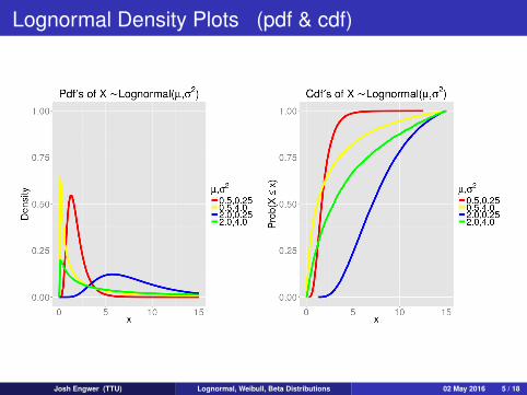
Lognormal Density Plots (pdf & cdf)
Josh Engwer (TTU) Lognormal, Weibull, Beta Distributions 02 May 2016 5 / 18

PART II
PART II:
WEIBULL DISTRIBUTION
Josh Engwer (TTU) Lognormal, Weibull, Beta Distributions 02 May 2016 6 / 18
Weibull Random Variables (Applications)
Weibull random variables reasonably model:
Lifetimes that are not memoryless:Lifetimes of certain electronicsLifetimes of certain mechanical devicesLifetimes of certain (biological) plantsLifetimes of certain animals
Sizes of particles resulting from grinding or crushing a materialWind speeds in weather forecastingTotal time from ordering a defective product to returning it
Josh Engwer (TTU) Lognormal, Weibull, Beta Distributions 02 May 2016 7 / 18
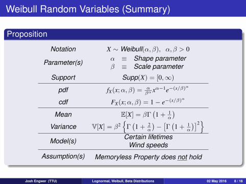
Weibull Random Variables (Summary)
Proposition
Notation X ∼Weibull(α, β), α, β > 0
Parameter(s) α ≡ Shape parameterβ ≡ Scale parameter
Support Supp(X) = [0,∞)
pdf fX(x;α, β) = αβα xα−1e−(x/β)α
cdf FX(x;α, β) = 1− e−(x/β)α
Mean E[X] = βΓ(1 + 1
α
)Variance V[X] = β2
{Γ(1 + 2
α
)−[Γ(1 + 1
α
)]2}Model(s) Certain lifetimes
Wind speeds
Assumption(s) Memoryless Property does not hold
Josh Engwer (TTU) Lognormal, Weibull, Beta Distributions 02 May 2016 8 / 18

Weibull Density Plots (pdf & cdf)
Josh Engwer (TTU) Lognormal, Weibull, Beta Distributions 02 May 2016 9 / 18
PART III
PART III:
BETA DISTRIBUTION
Josh Engwer (TTU) Lognormal, Weibull, Beta Distributions 02 May 2016 10 / 18

Beta Random Variables (Applications)
Beta random variables reasonably model proportions/percentages:
Proportions of some quantity in different samples:Proportion of some ingredient in a mixtureProportion of some mineral in a rockProportion of some nutrient in a plot of land soilRelative frequency of some gene in an animal populationTime allocation of tasks in a managerial project
Josh Engwer (TTU) Lognormal, Weibull, Beta Distributions 02 May 2016 11 / 18

The Beta Function B(α, β) (Definition & Properties)The beta function is a special function that routinely shows up in highermathematics, combinatorics, physics and (of course) statistics:
Definition(Beta Function)
The beta function is defined to be:
B(α, β) :=Γ(α)Γ(β)
Γ(α+ β), where α, β > 0
Moreover, the beta function possesses several useful properties:
Corollary(Useful Properties of the Beta Function)
B(α+ 1, β) =
(α
α+ β
)B(α, β)
B(α, β + 1) =
(β
α+ β
)B(α, β)
Josh Engwer (TTU) Lognormal, Weibull, Beta Distributions 02 May 2016 12 / 18
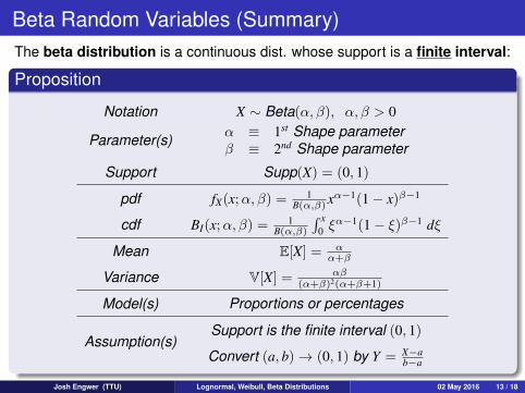
Beta Random Variables (Summary)The beta distribution is a continuous dist. whose support is a finite interval:
Proposition
Notation X ∼ Beta(α, β), α, β > 0
Parameter(s) α ≡ 1st Shape parameterβ ≡ 2nd Shape parameter
Support Supp(X) = (0, 1)
pdf fX(x;α, β) = 1B(α,β)xα−1(1− x)β−1
cdf BI(x;α, β) = 1B(α,β)
∫ x0 ξ
α−1(1− ξ)β−1 dξ
Mean E[X] = αα+β
Variance V[X] = αβ(α+β)2(α+β+1)
Model(s) Proportions or percentages
Assumption(s)Support is the finite interval (0, 1)
Convert (a, b)→ (0, 1) by Y = X−ab−a
Josh Engwer (TTU) Lognormal, Weibull, Beta Distributions 02 May 2016 13 / 18
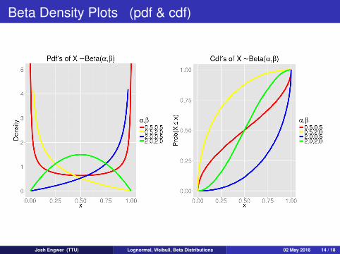
Beta Density Plots (pdf & cdf)
Josh Engwer (TTU) Lognormal, Weibull, Beta Distributions 02 May 2016 14 / 18

Computing Probabilities involving Beta r.v.’s
Let X ∼ Beta(α, β) ⇐⇒ pdf fX(x) =1
B(α, β)xα−1(1− x)β−1
Then, Prob(a ≤ X ≤ b) =
∫ b
afX(x) dx =
1B(α, β)
∫ b
axα−1(1− x)β−1 dx︸ ︷︷ ︸
Nonelementary integral!!
and the cdf isFX(x) = Prob(X ≤ x) = BI(x;α, β) =
1B(α, β)
∫ x
0ξα−1(1− ξ)β−1 dξ︸ ︷︷ ︸
Nonelementary integral!!
The problem with the Beta distribution is the resulting integrals have no finiteclosed-form anti-derivative when α, β are not integers!!If α, β are integers, tedious use of polynomial expansion is necessary!!
The fix to this is to numerically approximate the Beta cdf via a table.
Hence, use the table for the Beta cdf, which is called the incomplete Betafunction and is denoted BI(x;α, β).
Josh Engwer (TTU) Lognormal, Weibull, Beta Distributions 02 May 2016 15 / 18
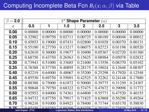
Computing Incomplete Beta Fcn BI(x;α, β) via Table
β = 2.0 1st Shape Parameter (α)x 0.5 1 1.5 2 2.5 3 3.5
0.00 0.00000 0.00000 0.00000 0.00000 0.00000 0.00000 0.000000.05 0.32982 0.09750 0.02711 0.00725 0.00189 0.00048 0.000120.10 0.45853 0.19000 0.07431 0.02800 0.01028 0.00370 0.001310.15 0.55190 0.27750 0.13217 0.06075 0.02723 0.01198 0.005200.20 0.62610 0.36000 0.19677 0.10400 0.05367 0.02720 0.013600.25 0.68750 0.43750 0.26563 0.15625 0.08984 0.05078 0.028320.30 0.73943 0.51000 0.33685 0.21600 0.13556 0.08370 0.051020.35 0.78388 0.57750 0.40895 0.28175 0.19024 0.12648 0.083070.40 0.82219 0.64000 0.48067 0.35200 0.25298 0.17920 0.125480.45 0.85530 0.69750 0.55091 0.42525 0.32262 0.24148 0.178800.50 0.88388 0.75000 0.61872 0.50000 0.39775 0.31250 0.243070.55 0.90848 0.79750 0.68322 0.57475 0.47672 0.39098 0.317720.60 0.92952 0.84000 0.74361 0.64800 0.55771 0.47520 0.401550.65 0.94732 0.87750 0.79917 0.71825 0.63868 0.56298 0.492640.70 0.96216 0.91000 0.84921 0.78400 0.71744 0.65170 0.588300.75 0.97428 0.93750 0.89309 0.84375 0.79160 0.73828 0.68504Josh Engwer (TTU) Lognormal, Weibull, Beta Distributions 02 May 2016 16 / 18
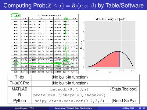
Computing Prob(X ≤ x) = BI(x;α, β) by Table/Software
TI-8x (No built-in function)TI-36X Pro (No built-in function)MATLAB betacdf(0.7,3,2) (Stats Toolbox)
R pbeta(q=0.7,shape1=3,shape2=2)
Python scipy.stats.beta.cdf(0.7,3,2) (Need SciPy)
Josh Engwer (TTU) Lognormal, Weibull, Beta Distributions 02 May 2016 17 / 18
Fin
Fin.
Josh Engwer (TTU) Lognormal, Weibull, Beta Distributions 02 May 2016 18 / 18


