Download - Merja Tornikoski Metsähovi Radio Observatory Single-dish blazar radio astronomy First lecture: Fundamentals of radio astronomy. Second lecture: Blazar

Merja TornikoskiMetsähovi Radio Observatory

Single-dish blazar radio astronomy

• First lecture: Fundamentals of radio astronomy.

• Second lecture: Blazar observing techniques.

• Third lecture: Radioastronomical blazar data into blazar science.


Radio astronomy

• Wavelength range ca. 100m – 100 m (MHz – THz).(Microwave/millimetre/submillimetre sub-regions).

• Broad frequency range: different kinds of antennae, receivers & technology!

• No (direct) images.• Signal usually << noise

emphasis on receiver technology and measurement methods.

• Terminology often differs from / contradicts with the terminology used in optical astronomy! (Historical and practical reasons).


Radio astronomical observations

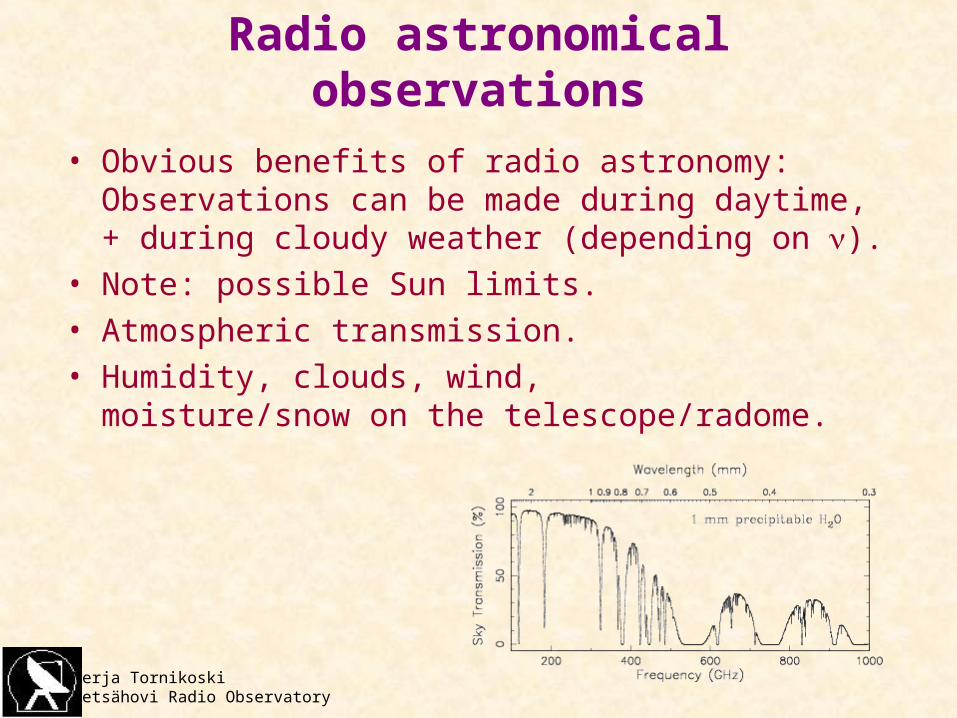
• Obvious benefits of radio astronomy:Observations can be made during daytime,+ during cloudy weather (depending on ).

• Note: possible Sun limits.• Atmospheric transmission.• Humidity, clouds, wind,

moisture/snow on the telescope/radome.


Radio astronomy in blazar science

• Dynamical events relatively close to the central engine (1-10 pc) radio flux monitoring, multifrequency radio data, multifrequency data.– Reasons for activity.– Energy production.– Reprocessing of energy.

• Flux data for larger source samples: unification models etc.

• Advantages:– Radio emission mechanism is relatively well understood

(synchrotron radiation from the jet/shock) helps in constraining/testing models also in other -domains.

– Dense sampling possible (daytime obs. etc.).– Natural part of the ”big picture”.


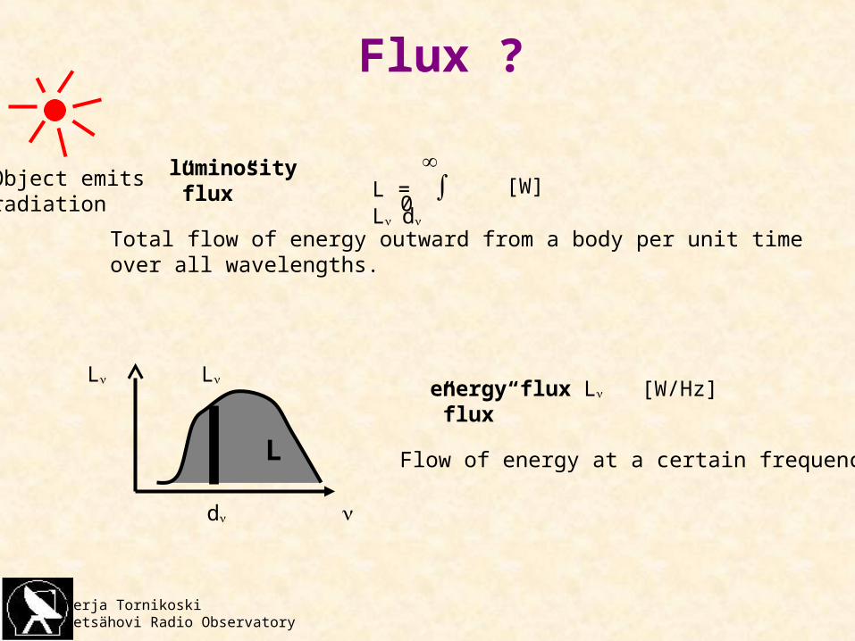
”Flux”?

Object emitsradiation

L [W/Hz]L

L

L

d

0

L = ∫ Ld [W]

luminosity”flux”

energy flux”flux”

Total flow of energy outward from a body per unit timeover all wavelengths.

Flow of energy at a certain frequency.


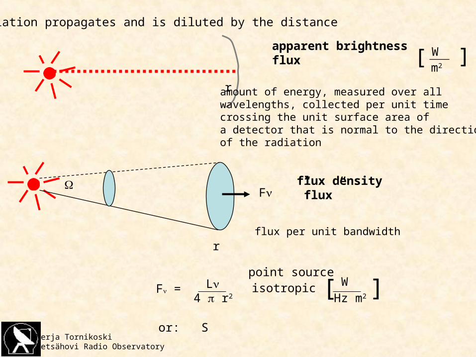
Radiation propagates and is diluted by the distance

r

F

F = L4 r2

isotropicHz m2

W[ ]

or: S

flux density”flux”

apparent brightnessflux

r

[ Wm2

]

point source

amount of energy, measured over all wavelengths, collected per unit time crossing the unit surface area of a detector that is normal to the direction of the radiation

flux per unit bandwidth


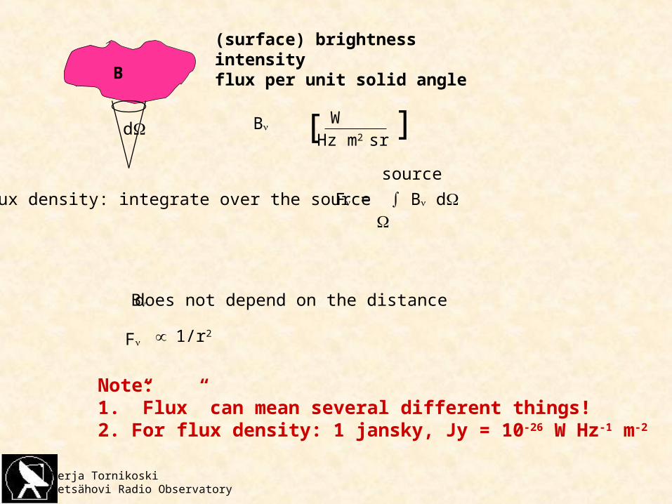
B

(surface) brightnessintensityflux per unit solid angle

BW

Hz m2 sr[ ]

flux density: integrate over the source F = ∫ B d

source

B

F

does not depend on the distance

1/r2

Note: 1. ”Flux” can mean several different things!2. For flux density: 1 jansky, Jy = 10-26 W Hz-1 m-2

d


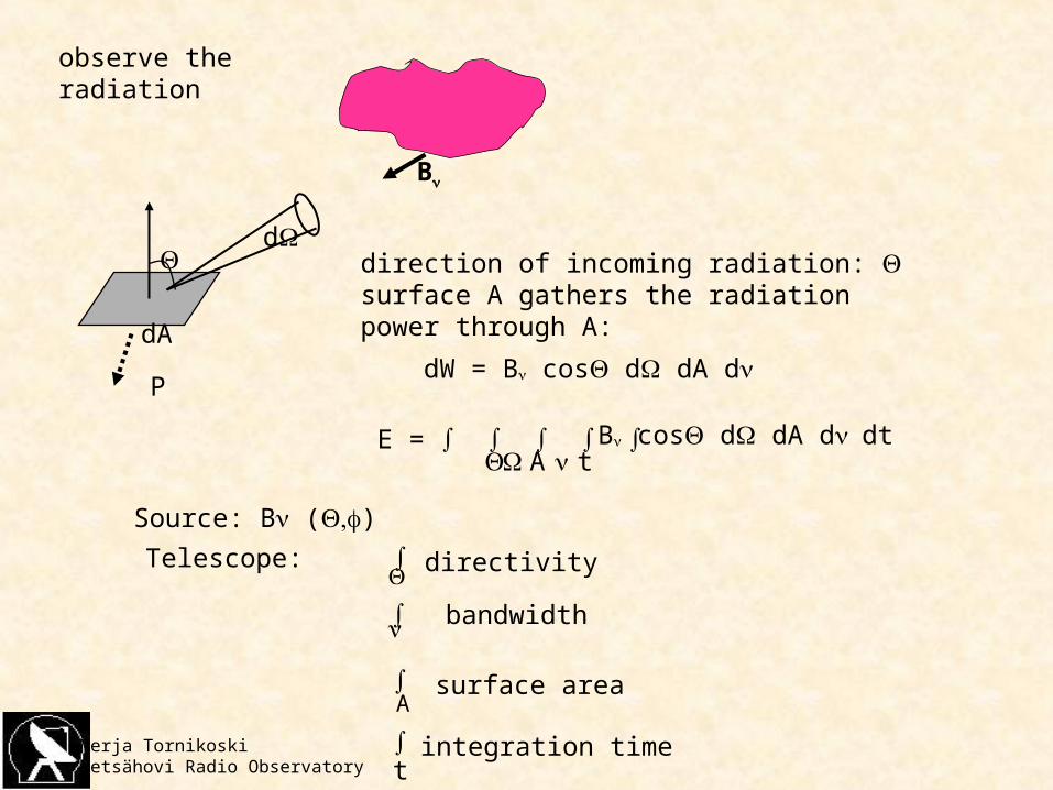
B

observe the radiation

d

dA

P

direction of incoming radiation: surface A gathers the radiationpower through A:

dW = B cos d dA d

E = ∫ ∫ ∫ ∫ ∫ B cos d dA ddt tA

Source: B ()

Telescope: ∫

∫

∫

∫

A

t

directivity

bandwidth

surface area

integration time


Black body radiation

• Ideal absorber and emitter, in thermal equilibrium.• Planck formula:

B(T)= 2 h 3/ (c2 (eh/kT-1))• For low frequencies: Rayleigh-Jeans approximation:

B(T)= 2 k T 2/ c2 = 2 k T / 2


Brightness temperature

• TB = the temperature that the source would have in order to produce the observed B.

• Does not need to be the physical temperature!

• Nyquist’s theorem: the corresponding derviation for the noise power flowing in a single-mode transmission line connected to a black body at temperature T leads to the one-dimensional analogue of the Planck law.

• Observing a black body or the sky/source:we observe the powerP d = k T d


Source brightness temperature

TS = B

2 k(Rayleigh-Jeans)

approximately equal to Tfys, if a black bodynot equal to Tfys otherwise! (Blazars!!!)


Radio telescope, antennae

• Radio telescopes are not limited by ”seeing”, but by the radiation pattern of the telescope.

• Radiation properties determined by refraction/reflection of electromagnetic radiation.

• Reciprocity principle:antenna’s transmission and reception properties are identical.

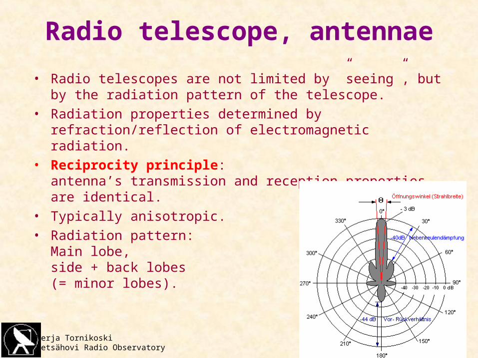
• Typically anisotropic.• Radiation pattern:

Main lobe,side + back lobes (= minor lobes).


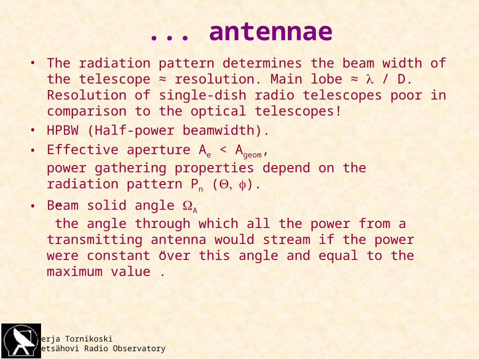
... antennae• The radiation pattern determines the beam width of the

telescope ≈ resolution. Main lobe ≈ / D.Resolution of single-dish radio telescopes poor in comparison to the optical telescopes!

• HPBW (Half-power beamwidth).

• Effective aperture Ae < Ageom,power gathering properties depend on the radiation pattern Pn ().

• Beam solid angle A ”the angle through which all the power from a transmitting antenna would stream if the power were constant over this angle and equal to the maximum value”.


... antennae

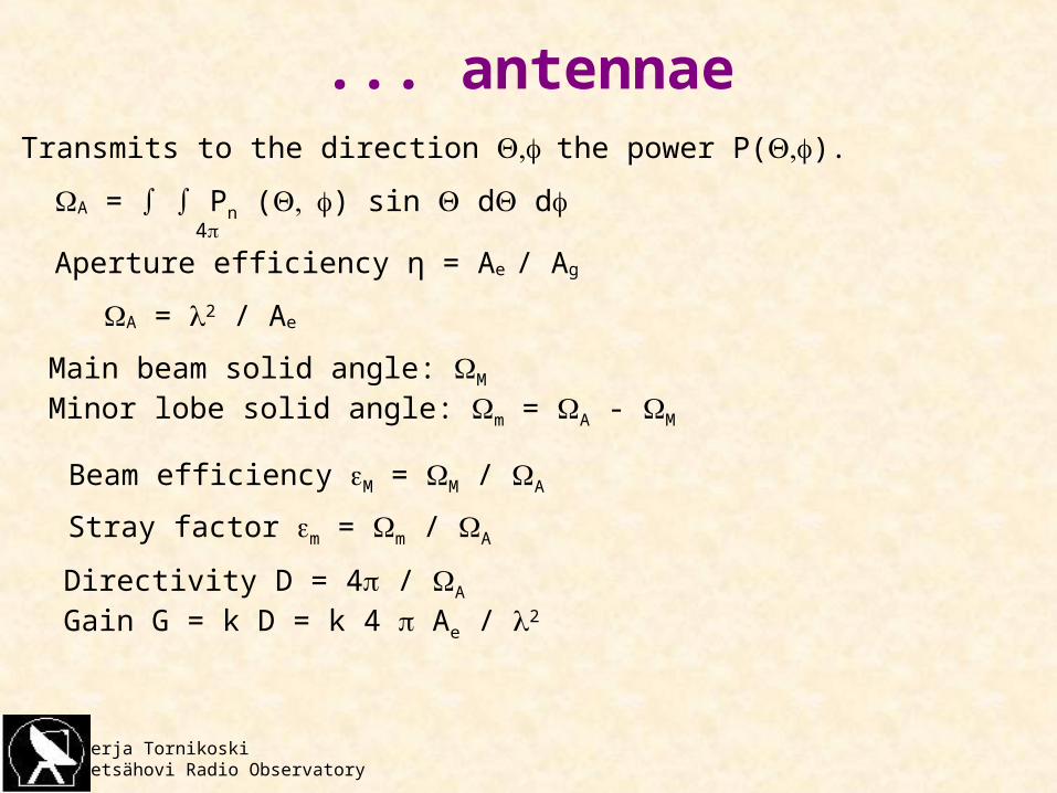
Aperture efficiency η = Ae / Ag

A = 2 / Ae

Main beam solid angle: M

Minor lobe solid angle: m = A - M

A = ∫ ∫ Pn () sin d d4

Transmits to the direction the power P().

Beam efficiency M = M / A

Stray factor m = m / A

Directivity D = 4 / A

Gain G = k D = k 4 Ae / 2


... antennae

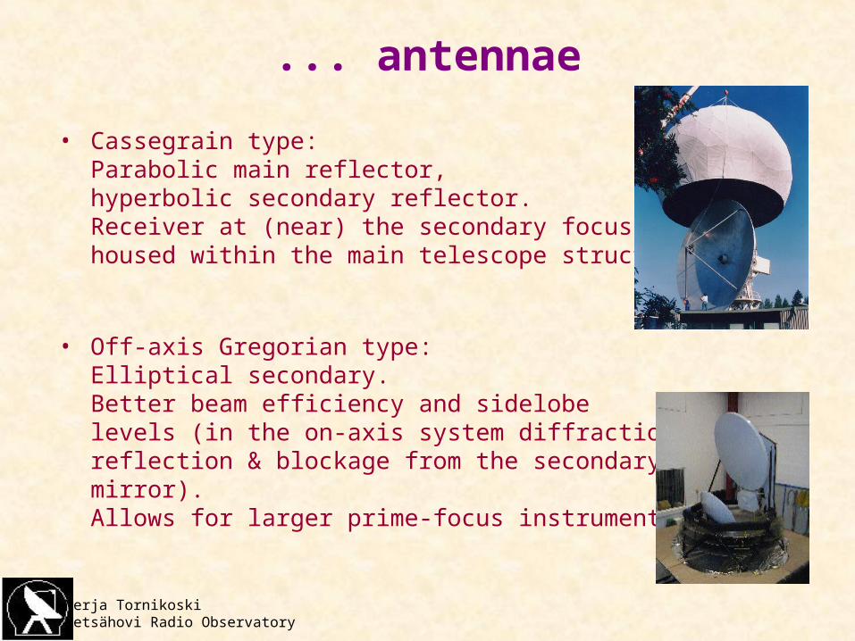
• Cassegrain type:Parabolic main reflector, hyperbolic secondary reflector.Receiver at (near) the secondary focus,housed within the main telescope structure.

• Off-axis Gregorian type:Elliptical secondary.Better beam efficiency and sidelobelevels (in the on-axis system diffraction,reflection & blockage from the secondarymirror).Allows for larger prime-focus instruments.


Surface accuracy/irregularities

• Good reflective characeristics.• Uniform shape over the entire area.• Uniform shape in different elevations.

• In reality, the shape is never perfect!– Gravitational forces.– Wind.– Heat: solar + other, panels + support structure.– Unevenness: panel installation, wearing out with

time, etc.


... surface accuracy

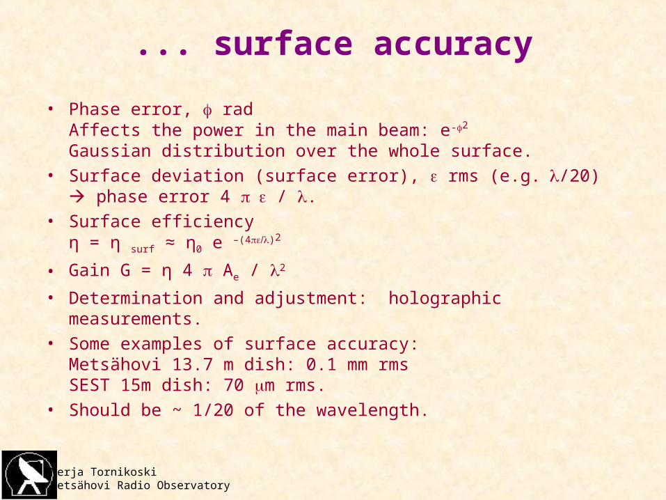
• Phase error, radAffects the power in the main beam: e-2

Gaussian distribution over the whole surface.• Surface deviation (surface error), rms (e.g./20)

phase error 4 / .• Surface efficiency

η = η surf ≈ η0 e –(4)2

• Gain G = η 4 Ae / 2

• Determination and adjustment: holographic measurements.• Some examples of surface accuracy:

Metsähovi 13.7 m dish: 0.1 mm rmsSEST 15m dish: 70 m rms.

• Should be ~ 1/20 of the wavelength.


Antenna temperature

• Antenna ”sees” a region of radiation through its directional pattern, the temperature of the region within the antenna beam determines the temperature of the radiation resistance. = Antenna temperature, TA.

• Not (directly) related to the physical temperature within the antenna structure!

• P = kTA [W/Hz].• The observed flux density (point source in the

beam)So = 2kTA / Ae


... Antenna temperature

• There are some second order effects to TA from physical temperature!

• Ae: Heat expansion Ae decreases, increases. Heat deformation η Ae

• Pn: Heat deformation.

• Tsys: Trx includes losses from the waveguides & transmission lines, may depend on the physical temperature.


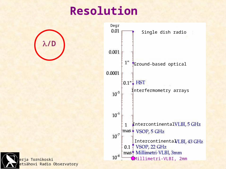
Resolution

Millimetri-VLBI, 2mm

/D

Degr

Single dish radio

Ground-based optical

Interfermometry arrays

Intercontinental

Intercontinental


Atmosphere

• Attenuattion.• Refraction.• Scattering.• Atmospheric emission.• ”Sky noise”.


... atmosphere

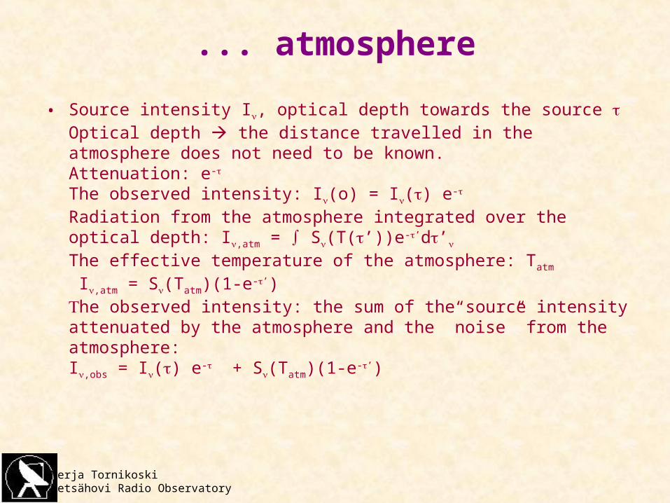
• Source intensity I, optical depth towards the source Optical depth the distance travelled in the atmosphere does not need to be known.Attenuation: e-

The observed intensity: I(o) = I() e-

Radiation from the atmosphere integrated over the optical depth: I,atm = ∫ S(T(’))e-’d’The effective temperature of the atmosphere: Tatm

I,atm = S(Tatm)(1-e-’)he observed intensity: the sum of the source intensity attenuated by the atmosphere and the ”noise” from the atmosphere:I,obs = I() e- + S(Tatm)(1-e-’)


... atmosphere

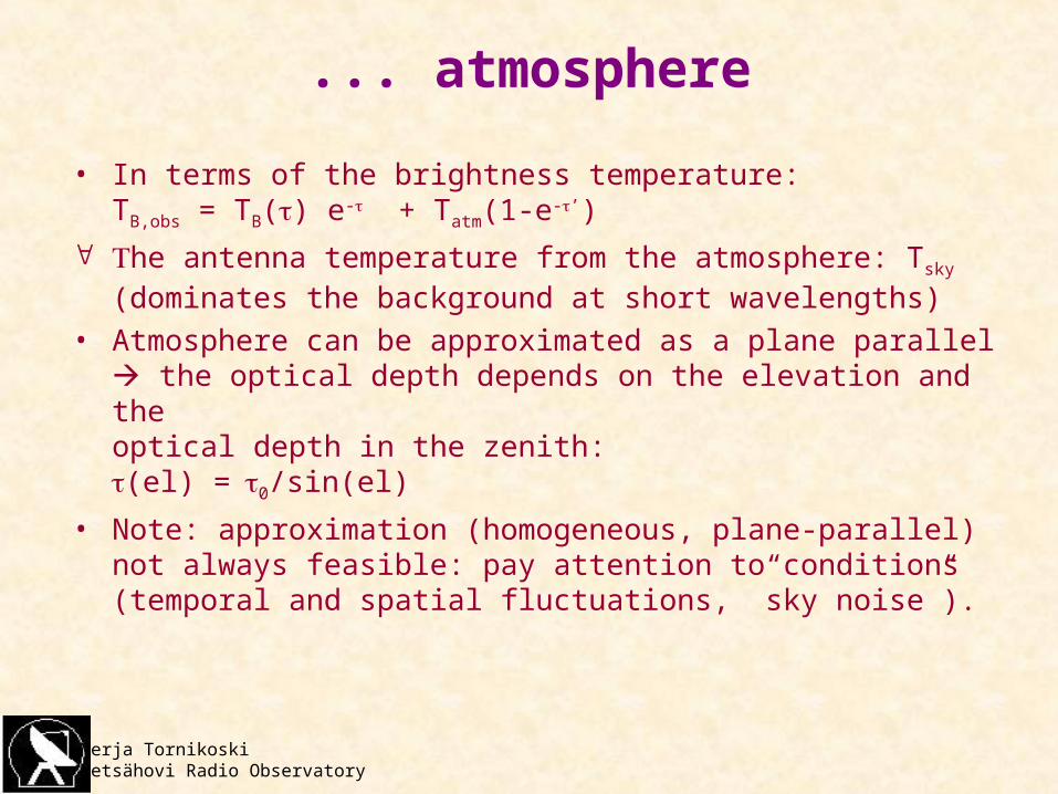
• In terms of the brightness temperature:TB,obs = TB() e- + Tatm(1-e-’)

he antenna temperature from the atmosphere: Tsky

(dominates the background at short wavelengths)• Atmosphere can be approximated as a plane parallel

the optical depth depends on the elevation and the optical depth in the zenith:(el) =0/sin(el)

• Note: approximation (homogeneous, plane-parallel) not always feasible: pay attention to conditions (temporal and spatial fluctuations, ”sky noise”).


Signal & noise

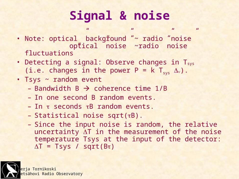
• Note: optical ”background” ~ radio ”noise” optical ”noise” ~radio ”noise fluctuations”

• Detecting a signal: Observe changes in Tsys

(i.e. changes in the power P = k Tsys ).• Tsys ~ random event

– Bandwidth B coherence time 1/B– In one second B random events.– In seconds B random events.– Statistical noise sqrt(B).– Since the input noise is random, the relative

uncertainty T in the measurement of the noise temperature Tsys at the input of the detector:T = Tsys / sqrt(B)


... signal & noise

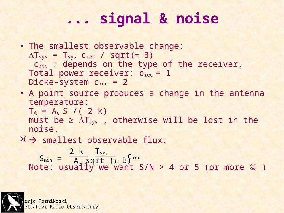
• The smallest observable change:Tsys = Tsys crec / sqrt( B) crec : depends on the type of the receiver,Total power receiver: crec = 1Dicke-system crec = 2

• A point source produces a change in the antenna temperature: TA = Ae S /( 2 k)must be ≥ Tsys , otherwise will be lost in the noise.

smallest observable flux:

Note: usually we want S/N > 4 or 5 (or more )Smin =

2 kAe

Tsys

sqrt ( B)crec


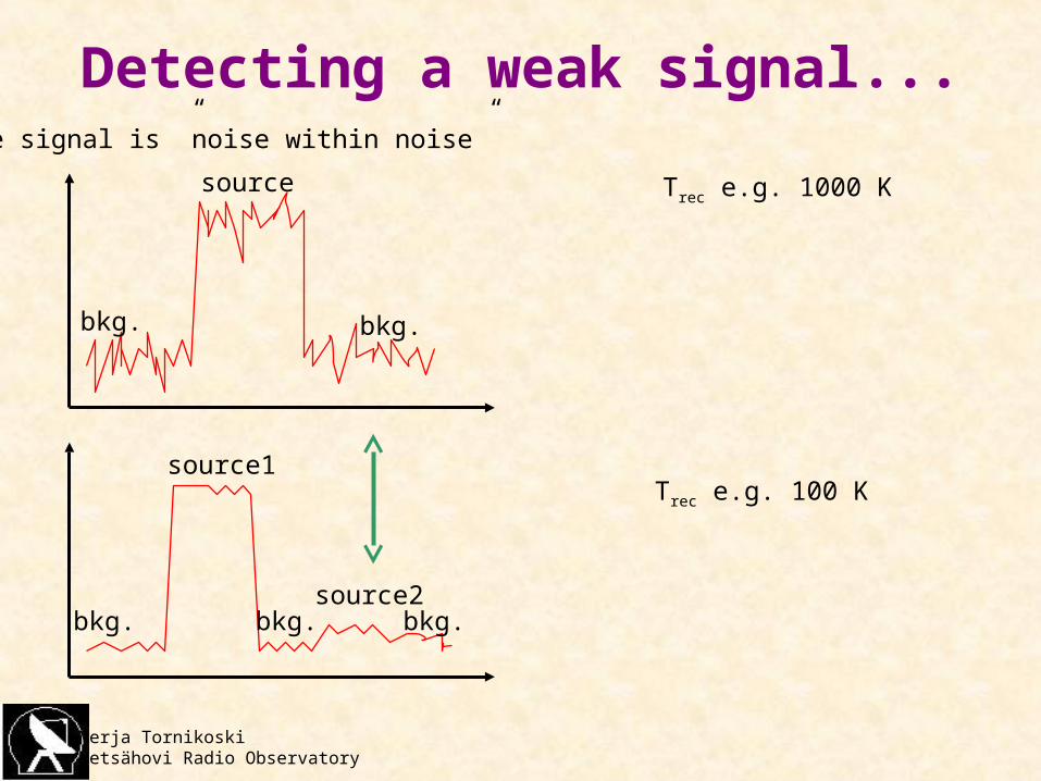
Detecting a weak signal...The signal is ”noise within noise”

Trec e.g. 1000 K

bkg. bkg.

source

Trec e.g. 100 K

bkg. bkg. bkg.

source1

source2


What we want...

• Large surface area Ae (”big & good antenna”).

• Small system temperature Tsys (”good, preferably cooled, receiver”).

• Broad-band receiver B(”continuum receiver, no sideband rejection”).

• Long integration time (”plenty of observing time”).

• Minimal attenuation & scatter, small skynoise effects(”perfect weather”).


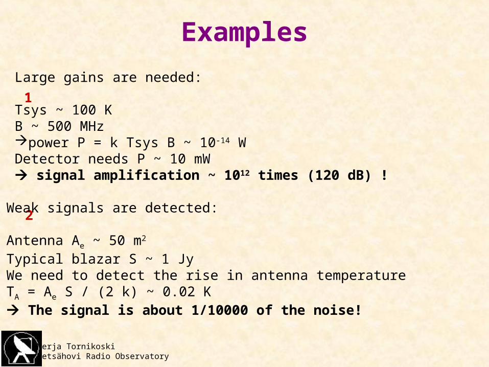
Examples

1

2

Large gains are needed:

Tsys ~ 100 KB ~ 500 MHzpower P = k Tsys B ~ 10-14 WDetector needs P ~ 10 mW signal amplification ~ 1012 times (120 dB) !

Weak signals are detected:

Antenna Ae ~ 50 m2

Typical blazar S ~ 1 JyWe need to detect the rise in antenna temperature TA = Ae S / (2 k) ~ 0.02 K The signal is about 1/10000 of the noise!


Future of radio astronomy?

• Radio frequencies are a ”natural resource” that must be ”conserved”!

• Radioastronomical use: passive use, active use means interference for us!

• < 30 GHz: 0.7% for ”primarily passive use”.

• 30-275 GHz: 3.0% for ”primarily passive use”.


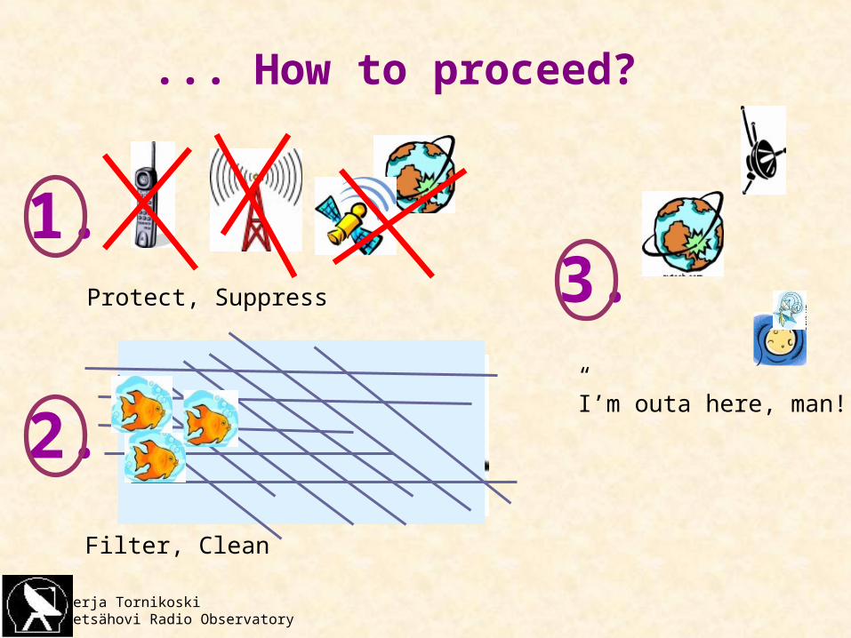
... How to proceed?

1.

2.

3.Protect, Suppress

Filter, Clean

”I’m outa here, man!”

Download - Merja Tornikoski Metsähovi Radio Observatory Single-dish blazar radio astronomy First lecture: Fundamentals of radio astronomy. Second lecture: Blazar

Top Related