
Shanghai | China | june | 2010 29th International Conference on Ocean, Offshore and Arctic Engineering 1
ANALYSIS METHODOLOGY OF VORTEX-INDUCED MOTIONS (VIM) ON A MONOCOLUMN PLATFORM APPLYING THE
HILBERT-HUANG TRANSFORM METHOD
june | 2010
Rodolfo T. Gonçalves
Guilherme R. Franzini
Guilherme F. Rosetti
André L. C. Fujarra
Kazuo Nishimoto
TPN – Numerical Offshore Tank
Department of Naval Architecture and Ocean
Engineering
Escola Politécnica – University of São Paulo
São Paulo, SP, Brazil
Shanghai | China | june | 2010 29th International Conference on Ocean, Offshore and Arctic Engineering 2
Introduction
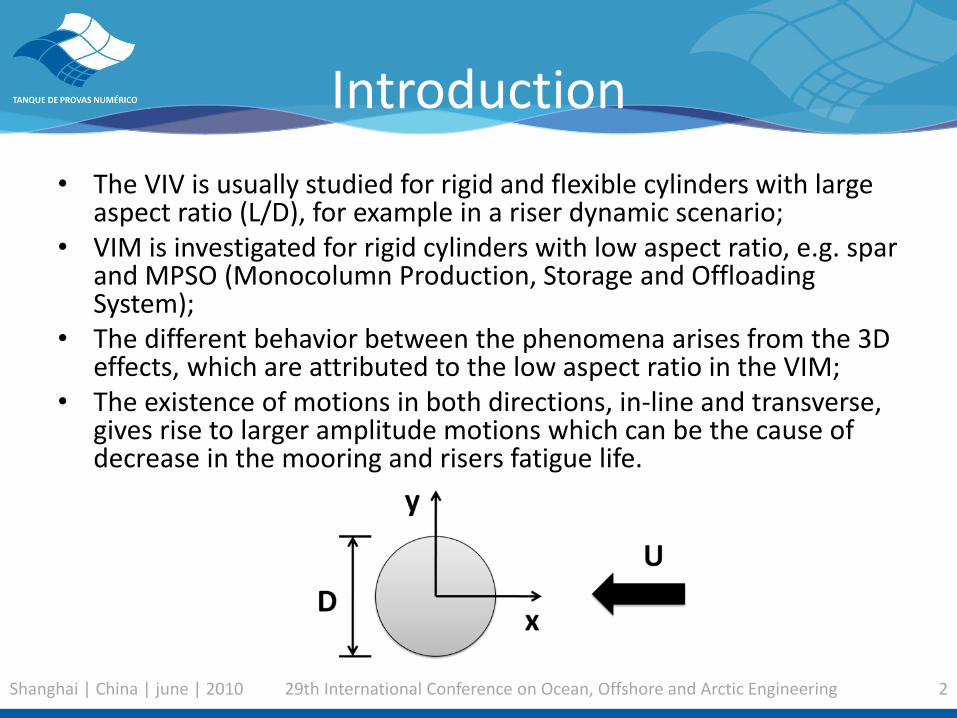
• The VIV is usually studied for rigid and flexible cylinders with large aspect ratio (L/D), for example in a riser dynamic scenario;
• VIM is investigated for rigid cylinders with low aspect ratio, e.g. spar and MPSO (Monocolumn Production, Storage and Offloading System);
• The different behavior between the phenomena arises from the 3D effects, which are attributed to the low aspect ratio in the VIM;
• The existence of motions in both directions, in-line and transverse, gives rise to larger amplitude motions which can be the cause of decrease in the mooring and risers fatigue life.

Shanghai | China | june | 2010 29th International Conference on Ocean, Offshore and Arctic Engineering 3
Motivation
• Experimental time-histories that emerge from VIM investigations are non-linear and non-stationary;
• Usual spectral analysis methods, based on Fourier Transform, rely on the hypotheses of linear and stationary dynamics;
• A method developed to treat non-stationary signals that originate from non-linear systems was presented by (Huang, et al., 1998). It is referred to as Hilbert-Huang transform method (HHT).
• The work proposes to create an analysis methodology to improve the statistics characteristics of VIM signal using the HHT.
Shanghai | China | june | 2010 29th International Conference on Ocean, Offshore and Arctic Engineering 4
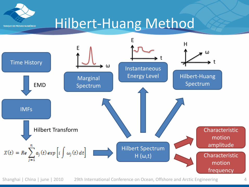
Hilbert-Huang Method
Time History
EMD
IMFs
Hilbert Transform
Hilbert Spectrum H (ω,t)
Marginal Spectrum
Instantaneous Energy Level Hilbert-Huang
Spectrum
Characteristic motion
amplitude
Characteristic motion
frequency
ω
E
t
E
t
ω H
Shanghai | China | june | 2010 29th International Conference on Ocean, Offshore and Arctic Engineering 5
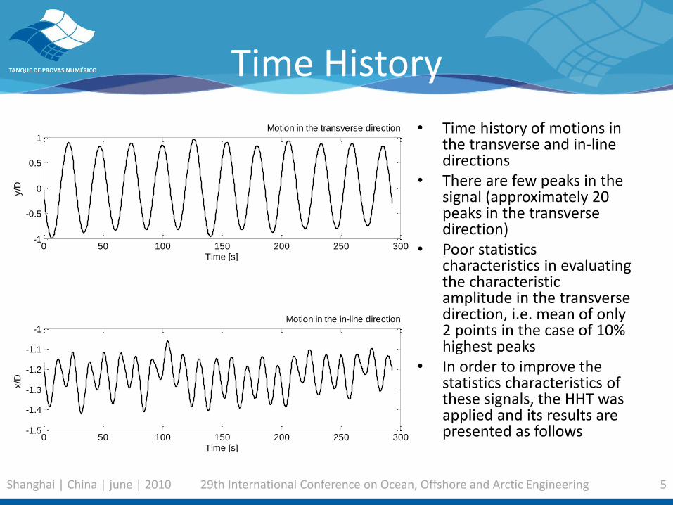
• Time history of motions in the transverse and in-line directions
• There are few peaks in the signal (approximately 20 peaks in the transverse direction)
• Poor statistics characteristics in evaluating the characteristic amplitude in the transverse direction, i.e. mean of only 2 points in the case of 10% highest peaks
• In order to improve the statistics characteristics of these signals, the HHT was applied and its results are presented as follows
Time History
0 50 100 150 200 250 300-1
-0.5
0
0.5
1
Time [s]
y/D
Motion in the transverse direction
0 0.05 0.10
10
20
30
40
50
Frequency [Hz]
Ma
rgin
al S
pe
ctr
um
0 100 200 3000
1
2
3
4
5x 10
-3
Insta
nta
ne
ou
s E
ne
rgy
Time [s]
0 50 100 150 200 250 300-1.5
-1.4
-1.3
-1.2
-1.1
-1
Time [s]
x/D
Motion in the in-line direction
0 0.05 0.10
0.5
1
1.5
2
Frequency [Hz]
Ma
rgin
al S
pe
ctr
um
0 100 200 3000
0.2
0.4
0.6
0.8
1
1.2x 10
-4
Insta
nta
ne
ou
s E
ne
rgy
Time [s]
Shanghai | China | june | 2010 29th International Conference on Ocean, Offshore and Arctic Engineering 6
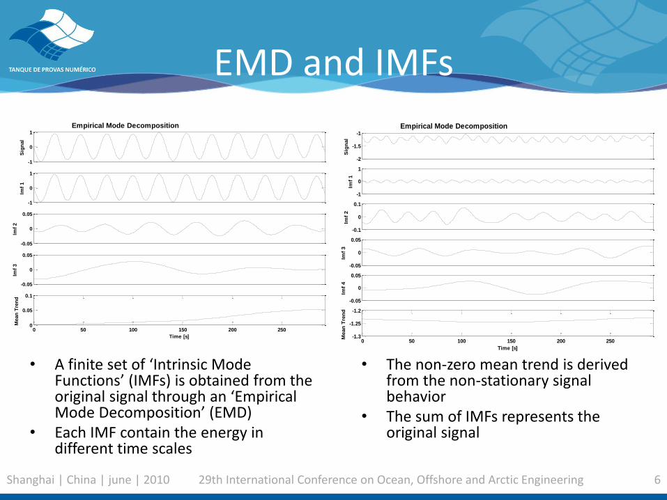
EMD and IMFs
• A finite set of ‘Intrinsic Mode Functions’ (IMFs) is obtained from the original signal through an ‘Empirical Mode Decomposition’ (EMD)
• Each IMF contain the energy in different time scales
-1
0
1
Sig
nal
Empirical Mode Decomposition
-1
0
1
Imf
1
-0.05
0
0.05
Imf
2
-0.05
0
0.05
Imf
3
0 50 100 150 200 2500
0.05
0.1
Time [s]
Mean
Tre
nd
-2
-1.5
-1
Sig
nal
Empirical Mode Decomposition
-1
0
1
Imf
1
-0.1
0
0.1
Imf
2
-0.05
0
0.05
Imf
3
-0.05
0
0.05
Imf
40 50 100 150 200 250
-1.3
-1.25
-1.2
Time [s]M
ean
Tre
nd
• The non-zero mean trend is derived from the non-stationary signal behavior
• The sum of IMFs represents the original signal

Shanghai | China | june | 2010 29th International Conference on Ocean, Offshore and Arctic Engineering 7
Hilbert-Huang Spectrum
• This frequency-time distribution of the amplitude is designated as the Hilbert spectrum
Time [s]
Fre
qu
en
cy [H
z]
Hilbert-Huang Spectrum
0 50 100 150 200 2500
0.01
0.02
0.03
0.04
0.05
0.06
0.07
0.08
0.09
0.1
Y/D
0.1
0.2
0.3
0.4
0.5
0.6
0.7
0.8
0.9
Time [s]
Fre
qu
en
cy [H
z]
Hilbert-Huang Spectrum
0 50 100 150 200 2500
0.01
0.02
0.03
0.04
0.05
0.06
0.07
0.08
0.09
0.1
X/D
0.02
0.04
0.06
0.08
0.1
0.12
0.14
0.16
0.18
• The frequency time-trace for the motions in the transverse direction is very energetic, but presents small fluctuations around 0.35 Hz.
• The frequency time-trace for the motions in the in-line direction has large fluctuation due to the highly non-stationary nature of the VIM.

Shanghai | China | june | 2010 29th International Conference on Ocean, Offshore and Arctic Engineering 8
Marginal Spectrum
• The marginal spectrum offers a measure of total amplitude (or energy) contribution from each frequency value. It is similar a the Power Spectrum by FFT
0 0.01 0.02 0.03 0.04 0.05 0.06 0.07 0.08 0.09 0.10
5
10
15
20
25
30
35
40
45
50
Frequency [Hz]
Ma
rgin
al S
pe
ctr
um
0 0.01 0.02 0.03 0.04 0.05 0.06 0.07 0.08 0.09 0.10
0.2
0.4
0.6
0.8
1
1.2
1.4
1.6
1.8
Frequency [Hz]
Ma
rgin
al S
pe
ctr
um
• The high energy level is comprised of a low width range of frequencies for the motions in the transverse direction, whereas the energy level is significant in a large width range for the motions in the in-line direction.

Shanghai | China | june | 2010 29th International Conference on Ocean, Offshore and Arctic Engineering 9
Intantaneous Energy Level
• The IE can be used to check the energy fluctuation over time, i.e. the amplitude modulation.
0 50 100 150 200 250 3000
0.5
1
1.5
2
2.5
3
3.5
4
4.5
5x 10
-3
Insta
nta
ne
ou
s E
ne
rgy
Time [s]0 50 100 150 200 250 300
0
0.2
0.4
0.6
0.8
1
1.2x 10
-4
Insta
nta
ne
ou
s E
ne
rgy
Time [s]
• The IE for the motions in the in-line direction is more irregular than the transverse direction ones. This fact confirms the high modulation amplitude present in the signal.

Shanghai | China | june | 2010 29th International Conference on Ocean, Offshore and Arctic Engineering 10
Characteristic Amplitudes
• The characteristic motion amplitude is evaluated applying the mean of the 10% largest amplitudes from H(ω,t).
• The characteristic motion frequency is the mean of the frequency related to the 10% largest amplitudes from H(ω,t).
0 2 4 6 8 10 12 14 160
0.2
0.4
0.6
0.8
1
Vr0
Y / D
Traditional AnalysisFujarra, et al. (2009)
HHT AnalysisGonçalves, et al. (2010)
0 2 4 6 8 10 12 14 160
0.05
0.1
0.15
0.2
Vr0
X / D
Traditional AnalysisFujarra, et al. (2009)
HHT AnalysisGonçalves, et al. (2010)
• The numbers of points to calculate the mean is proportional to the number of points in the signal time history, which provides a better statistics.
• The comparison between HHT and Traditional Analysis showed: • Small difference in the transverse
direction (around 2%) • Differences around 25% in the
in-line direction for Vr > 9.0

Shanghai | China | june | 2010 29th International Conference on Ocean, Offshore and Arctic Engineering 11
Conclusions
• The values of characteristic motion amplitudes showed to be more reliable owing to the large number of points to calculate the statistics using HHT.
• The comparison between traditional analysis (mean of the 10% highest peaks) and HHT analysis for VIM pointed out to larger differences observing the motion in the in-line direction. The difference is due to the non-stationary behavior of the VIM phenomenon (modulation in the amplitude and frequency).

Shanghai | China | june | 2010 29th International Conference on Ocean, Offshore and Arctic Engineering 12
THANKS


