Download - The Age of Graphical Computing
The Age of
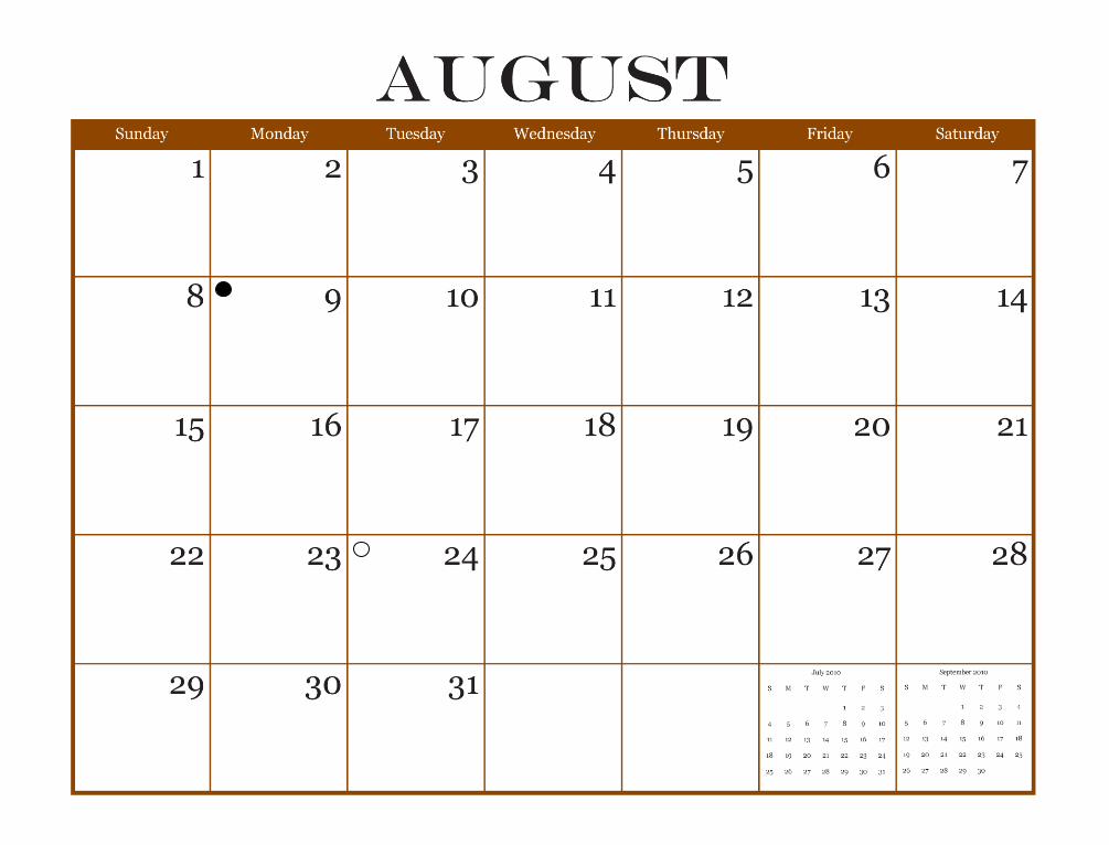
A 2010 Calendar
Graphical Computingy
A.D. 1844 A.D. 1974

Introduction
It is difficult for us today to grasp the drudgery of complex arithmetic calculations, or even repeated simpler calculations, in the past. This was especially true with repetitive computations that required tables of roots, logarithms and trigonometric functions in such fields as astronomy, navigation, surveying, and a wide variety of military and engineering applications.
Have you ever had to calculate the positions of astronomical objects? Orbital calculations relative to an observer on the Earth require derivations and time-consuming solutions of spherical trigonometric equations. And yet these kinds of calculations were accomplished by ancients such as Vitruvius and Ptolemy in the days prior to the advent of calculators or computers, or even trigonometry or algebra, using methods of Descriptive Geometry that are rarely taught today.
The Greeks folded (rabatted) the fundamental great circles onto the page and performed intricate geometrical constructions to map the Earth-Sun relative motion and incorporate local measurements into global maps and sophisticated sundials.
Astrolabes, quadrants and other volvelles and dials evolved to perform more complex computations in graphical form. In 1610-1614, Joost Bürgi and John Napier invented logarithms, and mathematicians and scientists such as Johann Kepler created tables of logarithms to aid in computation. William Oughtred and others developed the slide rule in the 1600s based on the properties of logarithms, and the slide rule continued its dominant role in non-graphical computation until the early 1970s. The slide rule provided the greatest versatility in computing the vast variety of equations, but it required multiple error-prone steps to provide solutions, effort that was not decreased even when solving one equation repetitively.
Meanwhile, on the graphical front Rene Descartes created the Cartesian coordinate system in the 17th century, and mathematicians over the next two centuries laid the foundation for applied numerical mathematics in large part on this field of analytical geometry. A two-dimensional graph provided fast solutions to an engineering precision for a single equation in two variables, and more complicated families of curves or so-called intersection charts extended the use of Cartesian graphs to one additional variable. T = 1.0
T = 1.1T = 1.2T = 1.3T = 1.4T = 1.5
T = 1.6
T = 1.7
T = 1.8
T = 1.9
T = 2.0
Introduction
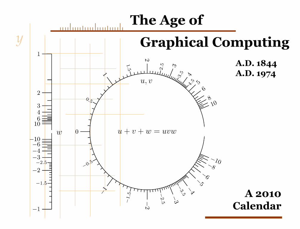
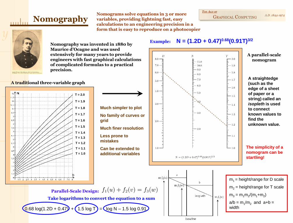
In 1844 Leon Lalanne succeeded in linearizing the curves y=xp by plotting the first log-log plot in history, thereby creating his Universal Calculator, chock-full of lines for common engineering calculations and capable of graphically computing formulas in powers or roots of x ( or of trigonometric functions in x) with ease. The year 1844 is taken here as the start of the Age of Graphical Computing. Other graphical methods evolved, and ultimately the field of nomography was invented in 1880 by Maurice d’Ocagne, a breakthrough in graphical computing so radical that it dominated the field of graphical computing until the spread of computers and electronic calculators in the early 1970s.
This 2010 calendar predominantly treats the field of nomography and the amazing variety of nomograms that can be created from it. A nomogram is a layout of graphical scales for computing formulas of 3 or more variables using a straightedge such as a ruler or the edge of a sheet of paper. A drawn or imagined isopleth connects matching values
Ron Doerfler
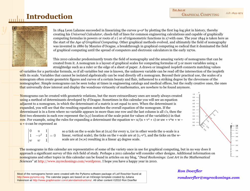
Nomograms can be created with geometric relations, but the more extraordinary ones are nearly always created using a method of determinants developed by d’Ocagne. Sometimes in this calendar you will see an equation adjacent to a nomogram, in which the determinant of a matrix is set equal to zero. When the determinant is expanded, you will see that the resulting equation matches the overall equation of the nomogram. If the determinant is in a form where no variable appears in more than one row and the last column is all 1’s, then the first two elements in each row represent the (x,y) location of the scale point for values of the variable(s) in that row. For example, using the rules for expanding a determinant the equation w= u/(u + v2 + 1) or uw + v2w + w –u = 0 can be expressed as
so a tick on the u-scale lies at (0,u) for every u, (or in other words the u-scale is a linear, vertical scale), the ticks on the v-scale are at (1,-v2), and the ticks on the w-scale are at (w,w) resulting in a linear 45 degree scale.
Most of the nomograms herein were created with the PyNomo software package of Leif Roschier found at
http://www.pynomo.org. The calendar pages are based on an InDesign template created by Juliana
Halvorson at http://www.graphmaster.com/calendarinstructions/. All other content ©2010 Ron Doerfler
of variables for a particular formula, so if all variables but one is known, the unknown variable can be read off the intersection of the isopleth with its scale. Variables that cannot be isolated algebraically can be read directly off a nomogram. Beyond their practical use, the scales of a nomogram often create geometric figures and curves of a certain beauty and flair, influenced to a striking degree by the cleverness of the nomographer. Simple nomograms can be seen today at times in engineering catalogs and medical offices, but the really creative ones, the ones that universally draw interest and display the wondrous virtuosity of mathematics, are nowhere to be found anymore.
The nomograms in this calendar are representative of some of the variety once in use for graphical computing, but in no way does it approach a significant survey of this rich field of study. Perhaps a 2011 calendar will consider other designs. Additional information on nomograms and other topics in this calendar can be found in articles on my blog, “Dead Reckonings: Lost Art in the Mathematical Sciences” at http://www.myreckonings.com/wordpress. I hope you have a happy year in 2010.
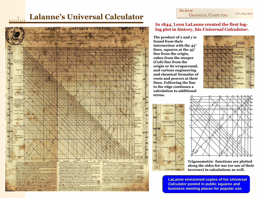
Lalanne’s Universal Calculator
LaLanne envisioned copies of his Universal
Calculator posted in public squares and
business meeting places for popular use.
In 1844, Leon LaLanne created the first log-log plot in history, his Universal Calculator.
The product of x and y is found from their intersection with the 45°lines, squares at the 45°line from the origin, cubes from the steeper (Cub) line from the origin or its wraparound, and various engineering and chemical formulas of roots and powers at their lines. Following the line to the edge continues a calculation to additional terms.
Trigonometric functions are plotted along the sides for use (or use of their inverses) in calculations as well.
New Year’s Day
Martin Luther King Day
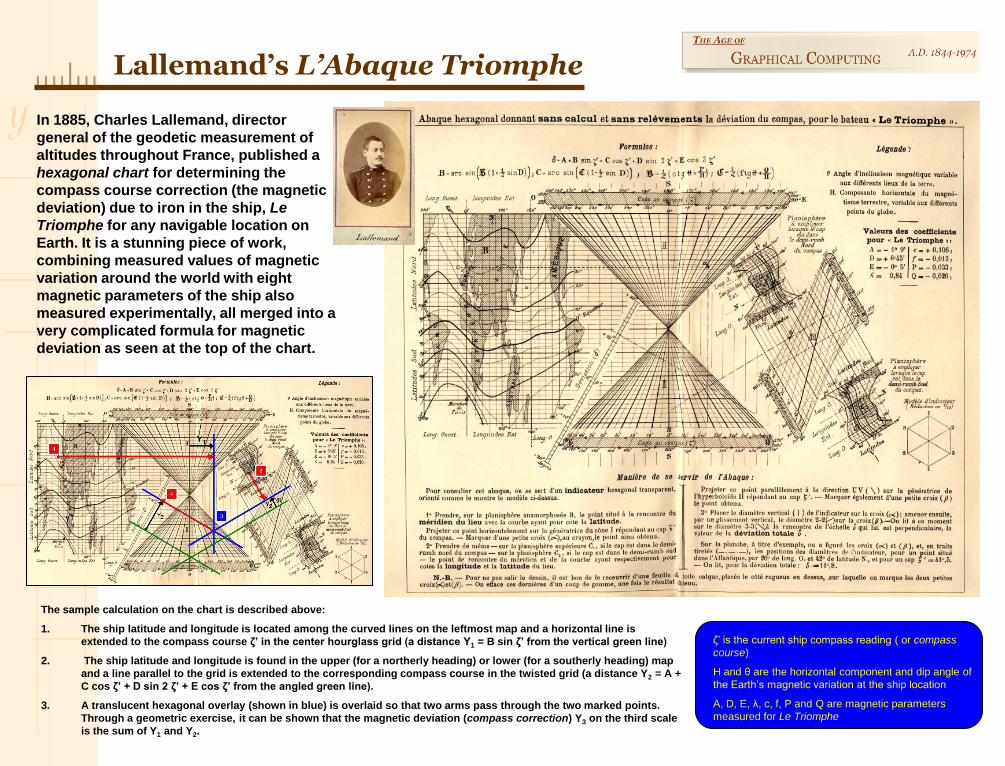
Lallemand’s L’Abaque Triomphe
In 1885, Charles Lallemand, director
general of the geodetic measurement of
altitudes throughout France, published a
hexagonal chart for determining the
compass course correction (the magnetic
deviation) due to iron in the ship, Le
Triomphe for any navigable location on
Earth. It is a stunning piece of work,
combining measured values of magnetic
variation around the world with eight
magnetic parameters of the ship also
measured experimentally, all merged into a
very complicated formula for magnetic
deviation as seen at the top of the chart.
The sample calculation on the chart is described above:
1. The ship latitude and longitude is located among the curved lines on the leftmost map and a horizontal line is
extended to the compass course ζ’ in the center hourglass grid (a distance Y1 = B sin ζ’ from the vertical green line)
2. The ship latitude and longitude is found in the upper (for a northerly heading) or lower (for a southerly heading) map
and a line parallel to the grid is extended to the corresponding compass course in the twisted grid (a distance Y2 = A +
C cos ζ’ + D sin 2 ζ’ + E cos ζ’ from the angled green line).
3. A translucent hexagonal overlay (shown in blue) is overlaid so that two arms pass through the two marked points.
Through a geometric exercise, it can be shown that the magnetic deviation (compass correction) Y3 on the third scale
is the sum of Y1 and Y2.
ζ’ is the current ship compass reading ( or compass
course)
H and θ are the horizontal component and dip angle of
the Earth’s magnetic variation at the ship location
A, D, E, λ, c, f, P and Q are magnetic parameters
measured for Le Triomphe
Valentine’s Day President’s Day
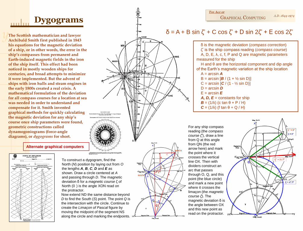
Dygograms
Now extend ND the same distance beyond
D to find the South (S) point. The point Q is
the intersection with the circle. Continue to
create the Limaçon of Pascal figure by
moving the midpoint of the segment NS
along the circle and marking the endpoints.
δ = A + B sin ζ’ + C cos ζ’ + D sin 2ζ’ + E cos 2ζ’
For any ship compass
reading (the compass
course ζ’), draw a line
from Q at this angle
from QN (the red
arrow here) and mark
the point where it
crosses the vertical
line OX. Then with
dividers construct an
arc that passes
through O, Q, and this
point (the blue circle)
and mark a new point
where it crosses the
limaçon (the magnetic
course ζ). The
magnetic deviation δ is
the angle between OX
and this new point as
read on the protractor.
δ is the magnetic deviation (compass correction)
ζ’ is the ship compass reading (compass course)
A, D, E, λ, c, f, P and Q are magnetic parameters
measured for the ship
H and θ are the horizontal component and dip angle
of the Earth’s magnetic variation at the ship location
A = arcsin A
B = arcsin [B / (1 + ½ sin D)]
C = arcsin [C / (1 - ½ sin D)]
D = arcsin D
E = arcsin E
A, D, E = constants for ship
B = (1/λ) (c tan θ + P / H)
C = (1/λ) (f tan θ + Q / H)
The Scottish mathematician and lawyer Archibald Smith first published in 1843 his equations for the magnetic deviation of a ship, or in other words, the error in the ship’s compasses from permanent and Earth-induced magnetic fields in the iron of the ship itself. This effect had been noticed in mostly wooden ships for centuries, and broad attempts to minimize it were implemented. But the advent of ships with iron hulls and steam engines in the early 1800s created a real crisis. A mathematical formulation of the deviation for all compass courses for a location at sea was needed in order to understand and compensate for it. Smith invented graphical methods for quickly calculating the magnetic deviation for any ship’s course once ship parameters were found, geometric constructions called dynamogoniograms (force-angle diagrams), or dygograms for short.
To construct a dygogram, find the
North (N) position by laying out from O
the lengths A, B, C, D and E as
shown. Draw a circle centered at A
and passing through D. The magnetic
deviation δ for a magnetic course ζ of
North (0 ) is the angle XON read on
the protractor.
Alternate graphical computers
Nomography
The simplicity of a
nomogram can be
startling!
Much simpler to plot
No family of curves or
grid
Much finer resolution
Less prone to
mistakes
Can be extended to
additional variables
A straightedge
(such as the
edge of a sheet
of paper or a
string) called an
isopleth is used
to connect
known values to
find the
unknown value.
Nomograms solve equations in 3 or more variables, providing lightning fast, easy calculations to an engineering precision in a form that is easy to reproduce on a photocopier
T = 1.0
T = 1.1
T = 1.2
T = 1.3
T = 1.4
T = 1.5
T = 1.6
T = 1.7
T = 1.8
T = 1.9
T = 2.0
A traditional three-variable graph
A parallel-scale nomogram
Example: N = (1.2D + 0.47)0.68(0.91T)3/2Nomography was invented in 1880 by Maurice d’Ocagne and was used extensively for many years to provide engineers with fast graphical calculations of complicated formulas to a practical precision.
Parallel-Scale Design:
m1 = height/range for D scale
m2 = height/range for T scale
m3 = m1m2/(m1+m2)
a/b = m1/m2 and a+b =
width0.68 log(1.2D + 0.47) + 1.5 log T = log N – 1.5 log 0.91
Take logarithms to convert the equation t0 a sum
Easter Sunday

Two Classic Nomogram Designs
A Concurrent-Scale Nomogram
where A is the angle between each of the 3 scales.
If A = 60° as below, then m1 = m2 = m3.
Standard resistor values can be marked so
a convenient combination can be found by
playing with the straightedge.
Here we have
r2 = V/πh
An “N” or “Z” ChartDesign:
The diagonal scale can be floating segment,
thus appearing “rather more spectacular” to
the casual observer [Douglass 1947].
Design:
Division Harmonic Relation

Mother’s Day
Memorial Day

Proportional Nomograms
True for all types shown here
Proportional Design:
4 Variable Proportion
Other Layouts
Father’s Day

Compound Linear Design:
Compound Nomograms
Equations of more than three variables can be graphically computed using compound nomograms sharing scales.
k
The middle solution scale of the concurrent nomogram
for two resistors in parallel can be used as the outer
scale of a second nomogram to extend the nomogram
for three resistors. A fourth parallel resistor can be
added by seesawing back through the first set of
scales, and so forth. A series resistor simply slides
upward along the scale.
Since the angle A between the
scales is 60 , the scales are
identical.
The k-scale is not labeled with scale
values. It is called a pivot line.

Independence Day Independence Day (Obs.)
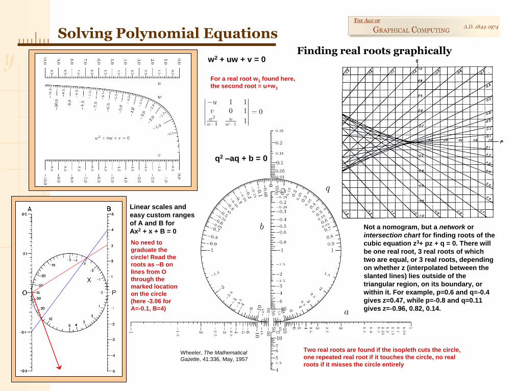
Solving Polynomial EquationsFinding real roots graphically
Linear scales and
easy custom ranges
of A and B for
Ax2 + x + B = 0
No need to
graduate the
circle! Read the
roots as –B on
lines from O
through the
marked location
on the circle
(here -3.06 for
A=-0.1, B=4)
Wheeler, The Mathematical
Gazette, 41:336, May, 1957
Two real roots are found if the isopleth cuts the circle,
one repeated real root if it touches the circle, no real
roots if it misses the circle entirely
For a real root w1 found here,
the second root = u+w1
Not a nomogram, but a network or
intersection chart for finding roots of the
cubic equation z3+ pz + q = 0. There will
be one real root, 3 real roots of which
two are equal, or 3 real roots, depending
on whether z (interpolated between the
slanted lines) lies outside of the
triangular region, on its boundary, or
within it. For example, p=0.6 and q=-0.4
gives z=0.47, while p=-0.8 and q=0.11
gives z=-0.96, 0.82, 0.14.
q2 –aq + b = 0
w2 + uw + v = 0

AstronomyOnce invented, nomogramswere soon applied to time-consuming and repetitive calculations in celestial mechanics
This is an example of a
nomogram solving for a
variable (φ) that cannot be
isolated algebraically.
nt = φ – e sin φ
Kepler’s Equation for the relation between the
polar angle φ of a celestial body in an eccentric
orbit and the time elapsed from an initial point
Celestial Parallax: the difference between
topocentric and geocentric location when
observing comets and minor planets. Done
with parallax correction, generally to two
digits and in great number to define the
orbits:
Δpα = parallax factor
πs = mean equatorial horizontal
parallax of the sun in seconds
ρ = Earth radius to observation
point in term of equatorial radius
φ = geocentric latitude of
observer
δ,H = declination and hour angle
of body
Kresàk, Bulletin of the
Astronomical Institute of
Czechoslovakia, 1957
after Leif Roschier—see
http://www.pynomo.org/wiki/index.php/Example:Star_navigation
Spherical Triangle relation between
declination, latitude, hour angle and azimuth
Spherical Triangle relation between
declination, latitude, altitude and azimuth

Labor Day

Navigation and Surveying
Friauf, Am. Math.
Monthly, 42:4, 1935
A 3D (4x4 determinant) nomogram
solution for Great Circle Distance
Here the φ-scale lies the same distance d above the paper as the L-scale lies
below it, but they are flattened to the paper. First, points A and B are joined by a
line. Then for a given L (point C), all four points will be coplanar if the point on the
flattened φ-scale is the same distance from AB as C and on a line parallel to AB.
A transparent overlay of parallel lines is used to find φ.
M. Collignon
sin φ – cos φ tan ε – ρ tan ε = 0
Angular correction for land surveys
Great Circle Distance
λ – λ’ = 25.2 °
λ + λ’ = 72.5 °
L = 116 °
φ = 87.5°
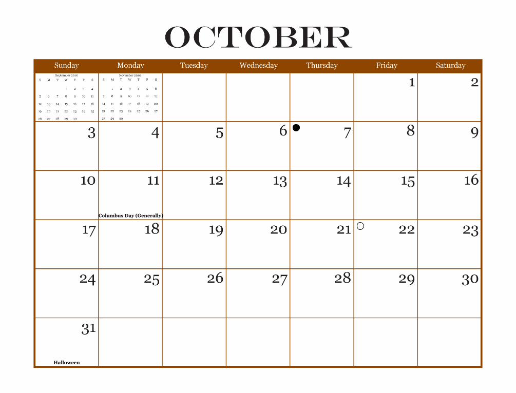
Columbus Day (Generally)
Halloween
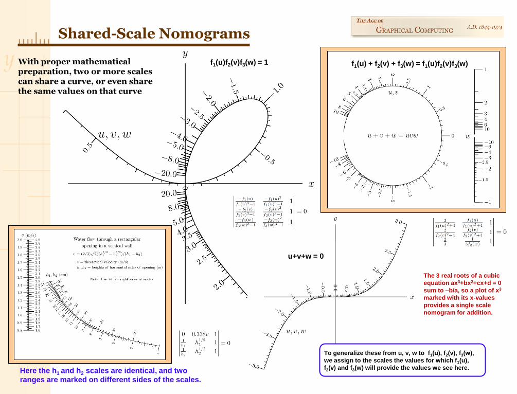
Shared-Scale Nomograms
Here the h1 and h2 scales are identical, and two
ranges are marked on different sides of the scales.
f1(u)f2(v)f3(w) = 1
The 3 real roots of a cubic
equation ax3+bx2+cx+d = 0
sum to –b/a, so a plot of x3
marked with its x-values
provides a single scale
nomogram for addition.
To generalize these from u, v, w to f1(u), f2(v), f3(w),
we assign to the scales the values for which f1(u),
f2(v) and f3(w) will provide the values we see here.
With proper mathematical preparation, two or more scales can share a curve, or even share the same values on that curve
f1(u) + f2(v) + f3(w) = f1(u)f2(v)f3(w)
u+v+w = 0

Election Day
Veteran’s Day
Thanksgiving
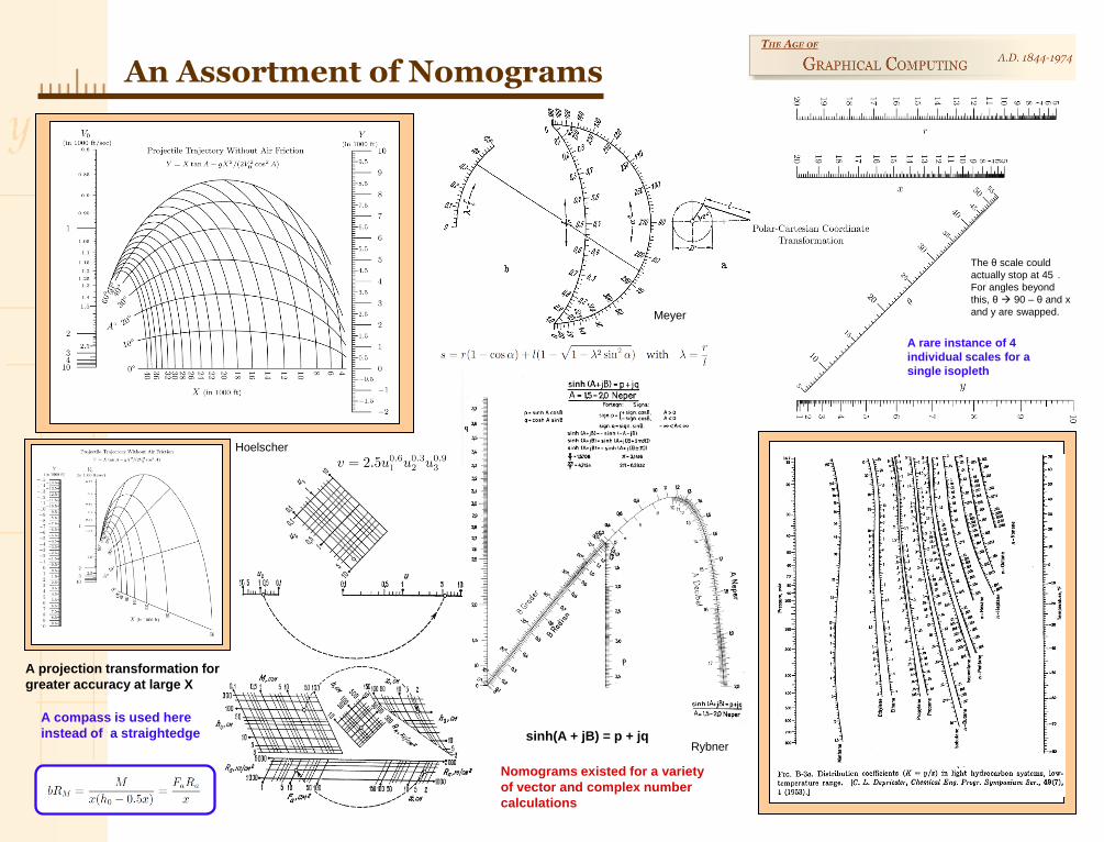
An Assortment of Nomograms
Nomograms existed for a variety
of vector and complex number
calculations
A compass is used here
instead of a straightedge
A projection transformation for
greater accuracy at large X
A rare instance of 4
individual scales for a
single isopleth
sinh(A + jB) = p + jqRybner
Hoelscher
Meyer
The θ scale could
actually stop at 45 .
For angles beyond
this, θ 90 – θ and x
and y are swapped.

Christmas DayChristmas Eve
New Year’s Eve

A 2010 Calendar of Graphical Computers
As a calculating aid graphical computers can solve very
complicated formulas with amazing ease.
As a curiosity graphical computers manifest the beauty
of mathematics in a highly visual, highly creative way.
Graphical Computers are fascinating artifacts in the history of mathematics. They possess an intrinsic charm well beyond their practical use.
Most of the nomograms herein were created with the PyNomo software package of Leif Roschier found
at http://www.pynomo.org. The calendar pages are based on an InDesign template created by Juliana
Halvorson at http://www.graphmaster.com/calendarinstructions/. All other content ©2010 Ron Doerfler
Contact: [email protected]


