Download - Thesis defense improved

Numerical methods for stochastic systems
subject to generalized Levy noiseby Mengdi Zheng!
Thesis committee: George Em Karniadakis (Ph.D., advisor)!Hui Wang (Ph.D., reader, APMA, Brown)!
Xiaoliang Wan (Ph.D., reader, Mathematics, LSU)

Motivation from 2 aspects
Mathematical!Reasons
Reasons from applications
Mathematical!Finance!
!Levy flights!in Chaotic!
flows

Goal of my thesisWe consider:!
!SPDEs driven by !
1. discrete RVs !2. jump processes!
!(jump systems/
memory systems)
Deterministic method:!!
Fokker-Planck (FP)!equation
Probabilistic method:!!
Monte Carlo (MC)!general Polynomial chaos (gPC)!
probability collocation method (PCM)!multi-element PCM (MEPCM)
Uncertainty !Quantification
We are the first ones who solved such systems through both deterministic & probabilistic methods.

Contents

Outline ♚ Adaptive multi-element polynomial chaos with discrete
measure: Algorithms and applications to SPDEs
♚ Adaptive Wick-Malliavin (WM) approximation to nonlinear
SPDEs with discrete RVs
♚ Numerical methods for SPDEs with 1D tempered -stable (T S) processes
♚ Numerical methods for SPDEs with additive multi-dimensional Levy jump processes
♚ Future work
αα

Probability collocation method (PCM) in UQXt (ω ) ≈ Xt (ξ1,ξ2,...,ξn ) ω ∈Ω Ε[um (x,t;ω )] ≈ Ε[um (x,t;ξ1,ξ2,...,ξn )]
ξ1
ξ2ξ3
... ξn
O Ω
PCM
ξ1
ξ2Ω
O
MEPCMB1 B2
B3 B4
n = 2
I = dΓ(x) f (x) ≈a
b
∫ dΓ(x) f (xi )hi (x)i=1
d
∑ = f (xi ) dΓ(x)hi (x)a
b
∫i=1
d
∑a
b
∫
Gauss integration:
u(x,t;ξ1i )i=1
d
∑ wi
n = 1
{Pi (x)}orthogonal to Γ(x)Pd (x)zeros of
Lagrange interpolation at zeros {xi ,i = 1,..,d}

Gauss quadrature and weights
generate orthogonal to{P j
k (ξj )}µ j (ξ j )
moment statistics
5 ways
tensor product
or sparse
grid
Ε[um (x,t;ω )]
017.5
3552.5
70
1 2 3 4
measure of
ξi
ξi
what if is a set of experimental data?ξi
subjective assumption of! distribution shapes
?ut + 6uux + uxxx = σ iξi ,
i=1
n
∑ x ∈!
u(x,0) = a2sech2 ( a
2(x − x0 ))
Data-driven UQ for stochastic KdV equations
M. Zheng, X. Wan, G.E. Karniadakis, Adaptive multi-element polynomial chaos with discrete measure: Algorithms and application to SPDEs, Applied Numerical Mathematics, 90 (2015), pp. 91–110.
A(k + n,n) = (−1)k+n−|i| n −1k + n− | i |
⎛⎝⎜
⎞⎠⎟(Ui1 ⊗ ...⊗Uin )
k+1≤|i|≤k+n∑
Sparse grids in Smolyak algorithm: level k, dimension n
sparse!grid
tensor!product!
grid

Construct orthogonal polynomials to discrete measures
1. (Nowak) S. Oladyshkin, W. Nowak, Data-driven uncertainty quantification using the arbitrary polynomial chaos expansion, Reliability Engineering & System Safety, 106 (2012), pp. 179–190.
2. (Stieltjes, Modified Chebyshev) W. Gautschi, On generating orthogonal polynomials, SIAM J. Sci. Stat. Comp., 3 (1982), no.3, pp. 289–317.
3. (Lanczos) D. Boley, G. H. Golub, A survey of matrix inverse eigenvalue problems, Inverse Problems, 3 (1987), pp. 595–622.
4. (Fischer) H. J. Fischer, On generating orthogonal polynomials for discrete measures, Z. Anal. Anwendungen, 17 (1998), pp. 183–205.
f (k;N , p) = N!k!(N − k)!
pk (1− p)N−k ,k = 0,1,...,N .
10 20 40 80 100
10−4
10−3
10−2
10−1
100
polynomial order i
CP
U ti
me
to e
valu
ate
orth
(i)
NowakStieltjesFischerModified ChebyshevLanczos
C*i2n=100,p=1/2
polynomial order i
Bino(100, 1/2)
0 10 20 30 40 50 60 70 80 90 100
10−20
10−15
10−10
10−5
100
polynomial order i
orth
(i)
NowakStieltjesFischerModified ChebyshevLanczos
N=100, p=1/2
polynomial order i
Bino(100, 1/2)
orthogonality ?
cost ?
Bino(N , p)Binomial distribution

| f (ξ )µ(ξ )− QmBi f
i=1
Nes
∑Γ∫ |≤Chm+1 || EΓ ||m+1,∞,Γ | f |m+1,∞,Γ
{Bi}i=1Nes : elementsNes : number of elements
: number of elementsΓµ : discrete measure
QmBi Gauss quadrature + tensor product with exactness m=2d-1
h: maximum size of Bi
f : test function in W m+1,∞(Γ)
(when the measure is continuous) J. Foo, X. Wan, G. E. Karniadakis, A multi-element probabilistic collocation method for PDEs with parametric uncertainty: error analysis and applications, Journal of Computational Physics 227 (2008), pp. 9572–9595.
Multi-element Gauss integration over discrete measures
2 3 4 5 6 7 8
10−3
10−2
d
error
l2u1aPCl2u2aPC
2 3 5 10 15 20 3010−7
10−6
10−5
10−4
10−3
10−2
Nes
error
l2u1
l2u2
C*Nel−4
h-convergence!of MEPCM
p-convergence of PCM
Poisson distribution
Binomial distribution

Adaptive MEPCM for stochastic KdV equation with 1RV
ut + 6uux + uxxx = σ iξi ,i=1
n
∑ x ∈!
u(x,0) = a2sech2 ( a
2(x − x0 ))
σ i2local variance to the measure µ(dξ ) / µ(dξ )
Bi∫
adaptive !integration!
mesh
2 3 4 5 6
10−5
10−4
10−3
10−2
Number of PCM points on each element
erro
rs
2 el, even grid2 el, uneven grid4 el, even grid4 el, uneven grid5 el, even grid5 el, uneven grid
(MEPCM)!adaptive!
vs.!non-
adaptive!meshes
error of Ε[u2 ]
Improved !

ut + 6uux + uxxx = σ iξi ,i=1
n
∑ x ∈!
u(x,0) = a2sech2 ( a
2(x − x0 ))
(sparse grid) D. Xiu, J. S. Hesthaven, High-order collocation methods for differential equations with random inputs, SIAM J. Scientific Computing 27(3) (2005), pp. 1118– 1139.
17 153 256 969 4,84510−10
10−9
10−8
10−7
10−6
10−5
10−4
r(k)
erro
rs
l2u1(sparse grid)
l2u2(sparse grid)
l2u1(tensor product grid)
l2u2(tensor product grid)
sparse grid vs. tensor product grid
Binomial distribution
n=8
Improved !
2D sparse grid in Smolyak algorithm
UQ of stochastic KdV equation with multiple RVs

Summary of contributions (1)
✰ convergence study of multi-element integration over discrete measure
!✰ comparison of 5 ways to construct orthogonal
polynomials w.r.t. discrete measure !✰ improvement of moment statistics by adaptive
integration mesh (on discrete measure) !✰ improvement of efficiency in computing moment
statistics by sparse grid (on discrete measure)

Outline ♚ Adaptive multi-element polynomial chaos with discrete
measure: Algorithms and applications to SPDEs
♚ Adaptive Wick-Malliavin (WM) approximation to
nonlinear SPDEs with discrete RVs
♚ Numerical methods for SPDEs with 1D tempered -stable (T S) processes
♚ Numerical methods for SPDEs with additive multi-dimensional Levy jump processes
♚ Future work
αα

gPC for 1D stochastic Burgers equation
M. Zheng, B. Rozovsky, G.E. Karniadakis, Adaptive Wick-Malliavin Approximation to Nonlinear SPDEs with Discrete Random Variables, SIAM J. Sci. Comput., revised. (multiple discrete RVs)
D. Venturi, X. Wan, R. Mikulevicius, B.L. Rozovskii, G.E. Karniadakis, Wick-Malliavin approximation to nonlinear stochastic PDEs: analysis and simulations, Proceedings of the Royal Society, vol.469, no.2158, (2013). (multiple Gaussian RVs)
ut + uux =υuxx +σ c1(ξ;λ), x ∈[−π ,π ]
u(x,t;ξ ) ≈ u! k (x,t)ck (ξ;λ)k=0
P
∑Expand the solution:
∂u! k∂t
+ u! m∂u! n∂t
< cmcnck >=m,n=0
P
∑ υ ∂2u! k∂x2
+σδ1k ,
general Polynomial Chaos (gPC) propagator
k = 0,1,...,P.
ξ ∼ Pois(λ)
ck : Charlier polynomiale−λλ k
k!cm (k;λ)cn (k;λ) =< cmcn >= n!λ
nδmnk∈!∑
cm
by Galerkin projection : < uck >
nonlinear
How many numbers of terms !!!!there are !
u! m∂u! n∂t
< cmcnck >
?
(motivation)
Let us simplify the gPC propagator !
(P +1)3

Wick-Malliavin (WM) approximation
G.C. Wick, The evaluation of the collision matrix, Phys. Rev. 80 (2), (1950), pp. 268-272.
◊
ξ ∼ Pois(λ)✰ consider with measure !✰ define Wick product as: ✰ define Malliavin derivative D as: !✰ the product of two polynomials can be approximated by: !!!✰ here
!✰ approximate the product of uv as:
Γ(x) = e−λλ k
k!δ (x − k)
k∈!∑
cm (x;λ)◊cn (x;λ) = cm+n (x;λ),
Dpci (x;λ) =i!
(i − p)!ci−p (x;λ)
cm (x)cm (x) = a(k,m,n)ck (x) =k=0
m+n
∑ Kmnpcm+n−2 p (x;λ)p=0
m+n2
∑Kmnp = a(m + n − 2p,m,n)
uv =Dpu◊ pD
pvp!
≈p=0
∞
∑ Dpu◊ pDpv
p!p=0
Q
∑

WM approximation simplifies the gPC propagator !ut + uux =υuxx +σ c1(ξ;λ), x ∈[−π ,π ]
∂u! k∂t
+ u! m∂u! n∂t
< cmcnck >=m,n=0
P
∑ υ ∂2u! k∂x2
+σδ1k , k = 0,1,...,P.gPC propagator:
∂u! k∂t
+ u! ii=0
P
∑ ∂u! k+2 p−i∂x
Ki,k+2 p−i,Q =p=0
Q
∑ υ ∂2u! k∂x2
+σδ1k , k = 0,1,...,P.WM propagator:
How much less? Let us count the dots !
k=0 k=1 k=2 k=3 k=4
P=4, Q=1/2
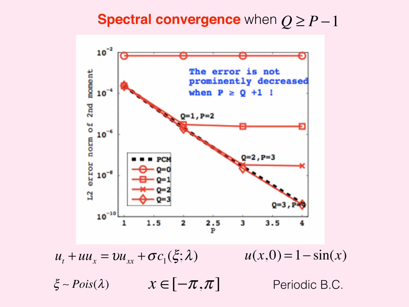
Spectral convergence when Q ≥ P −1
ut + uux =υuxx +σ c1(ξ;λ) u(x,0) = 1− sin(x)
ξ ∼ Pois(λ) x ∈[−π ,π ] Periodic B.C.

concept of P-Q refinement
ut + uux =υuxx +σ c1(ξ;λ) u(x,0) = 1− sin(x)
ξ ∼ Pois(λ) x ∈[−π ,π ] Periodic B.C.

WM for stochastic Burgers equation w/ multiple RVs
ut + uux =υuxx +σj=1
3
∑ c1(ξ j;λ)cos(0.1 jt)
0.2 0.3 0.4 0.5 0.6 0.7 0.8 0.9 110−7
10−6
10−5
10−4
10−3
10−2
T
l2u2(T)
Q1=Q2=Q3=0
Q1=1,Q2=Q3=0
Q1=Q2=1,Q3=0
Q1=Q2=Q3=1
u(x,0) = 1− sin(x) ξ1,2,3 ∼ Pois(λ)
x ∈[−π ,π ] Periodic B.C.
How about 3 discrete RVs ? How about the cost in d-dim ?
C(P,Q)d the # of terms u! i∂u! j∂x
(P +1)3d the # of terms u! m∂u! n∂t
Let us find the ratio C(P,Q)d
(P +1)3d
P=3 Q=2
P=4 Q=3
d=2 61.0% 65.3%
d=3 47.7% 52.8%
d=4 0.000436% 0.0023%
C(P,Q)d
(P +1)3d
??
Cost: WM vs. gPC

Summary of contributions (2)
References
✰ Extend the numerical work on WM approximation for SPDEs driven by Gaussian RVs to discrete RVs with arbitrary distribution w/ finite moments
✰ Discover spectral convergence when for stochastic Burgers equations
✰ Error control with P-Q refinements ✰ Computational complexity comparison of gPC and
WM in d dimensions
Q ≥ P −1
D. Bell, The Malliavin calculus, Dover, (2007)
S. Kaligotla and S.V. Lototsky, Wick product in the stochastic Burgers equation: a curse or a cure? Asymptotic Analysis 75, (2011), pp. 145–168.
S.V. Lototsky, B.L. Rozovskii, and D. Selesi, On generalized Malliavin calculus, Stochastic Processes and their Applications 122(3), (2012), pp. 808–843.
R. Mikulevicius and B.L. Rozovskii, On distribution free Skorokhod-Malliavin calculus, submitted.

Outline ♚ Adaptive multi-element polynomial chaos with discrete
measure: Algorithms and applications to SPDEs
♚ Adaptive Wick-Malliavin (WM) approximation to nonlinear
SPDEs with discrete RVs
♚ Numerical methods for SPDEs with 1D tempered -stable (T S) processes
♚ Numerical methods for SPDEs with additive multi-dimensional Levy jump processes
♚ Future work
αα

sample path of a Poisson process
Jt
t
Introduction of Levy processes

M. Zheng, G.E. Karniadakis, ‘Numerical Methods for SPDEs with Tempered Stable Processes’,SIAM J. Sci. Comput., accepted.
N. Hilber, O. Reichmann, Ch. Schwab, Ch. Winter, Computational Methods for Quantitative Finance: Finite Element Methods for Derivative Pricing, Springer Finance, 2013.
S.I. Denisov, W. Horsthemke, P. Ha ̈nggi, Generalized Fokker-Planck equation: Derivation and exact solutions, Eur. Phys. J. B, 68
(2009), pp. 567–575.
Generalized Fokker-Planck Equation for Overdamped Langevin EquationOverdamped Langevin equation (1D, SODE, in the Ito’s sense)
Density satisfies tempered fractional PDEs (by Ito’s formula)
1D tempered stable (TS) pure jump process has this Levy measure

Generalized FP Equation for Overdamped Langevin Equation w/ TS white noise
Left Riemann-Liouville tempered fractional derivatives (as an example)
Fully implicit scheme in time, Grunwald-Letnikov for fractional derivatives
MC for Overdamped Langevin Equation driven by TS white noise
TFPDE
PCM for Overdamped Langevin Equation driven by TS white noise
Compound Poisson (CP) approximation
MC!(probabilistic)
PCM!(probabilistic)
TFPDE!(deterministic)
1
23

Histogram from MC vs. Density from TFPDEs
jump intensity jump size distribution

Moment Statistics from PCM/CP vs. TFPDE
1. TFPDE costs less than PCM 2. PCM depends on the series representation 3. TFPDE depends on the initial condition 4. Convergence in TFPDE by refinement
λ = 10 λ = 1

Outline ♚ Adaptive multi-element polynomial chaos with discrete
measure: Algorithms and applications to SPDEs
♚ Adaptive Wick-Malliavin (WM) approximation to nonlinear
SPDEs with discrete RVs
♚ Numerical methods for SPDEs with 1D tempered -stable (T S) processes
♚ Numerical methods for SPDEs with additive multi-dimensional Levy jump processes
♚ Future work
αα

M. Zheng, G.E. Karniadakis, Numerical methods for SPDEs with additive multi-dimensional Levy jump processes, in preparation.

How to describe the dependence structure among components!of a multi-dimensional Levy jump process ?
LePage’s representation of Levy measure:1Series representation:
Levy measure:
J. Rosinski, Series representations of Levy processes from the perspective of point processes in: Levy Processes - Theory and Applications, O. E. Barndor-Nielsen, T. Mikosch and S. I. Resnick (Eds.), Birkh ̈auser, Boston, (2001), pp. 401–415.

How to describe the dependence structure among components!of a multi-dimensional Levy jump process ?
Dependence structure by Levy copula:
J. Kallsen, P. Tankov, Characterization of dependence of multidimensional Levy processes using Levy copulas, Journal of Multivariate Analysis, 97 (2006), pp. 1551–1572.
Levy copula + Marginal Levy measure = Levy measure
Series rep:
τ = 1
τ = 100
Construction:
2

Analysis of variance (ANOVA) + FP = marginal distributionFP equation
ANOVA decomposition
ANOVA terms are related to marginal distributions
1D-ANOVA-FP for marginal distributions
2D-ANOVA-FP for marginal distributionsLePage’s representation
TFPDEs
0 0.2 0.4 0.6 0.8 1−2
0
2
4
6
8
10
12
x
E[u(
x,T=
1)]
E[uPCM]
E[u1D−ANOVA−FP]
E[u2D−ANOVA−FP]
0.6 0.65 0.7 0.75 0.8 0.85 0.9 0.95 13.4
3.6
3.8
4
4.2
4.4
4.6
4.8
5
5.2x 10⁻⁴
T
L 2 nor
m o
f diff
eren
ce in
E[u
]
||E[u1D−ANOVA−FP−E[uPCM]||L2([0,1])/||E[uPCM]||L2([0,1])
||E[u2D−ANOVA−FP−E[uPCM]||L2([0,1])/||E[uPCM]||L2([0,1])
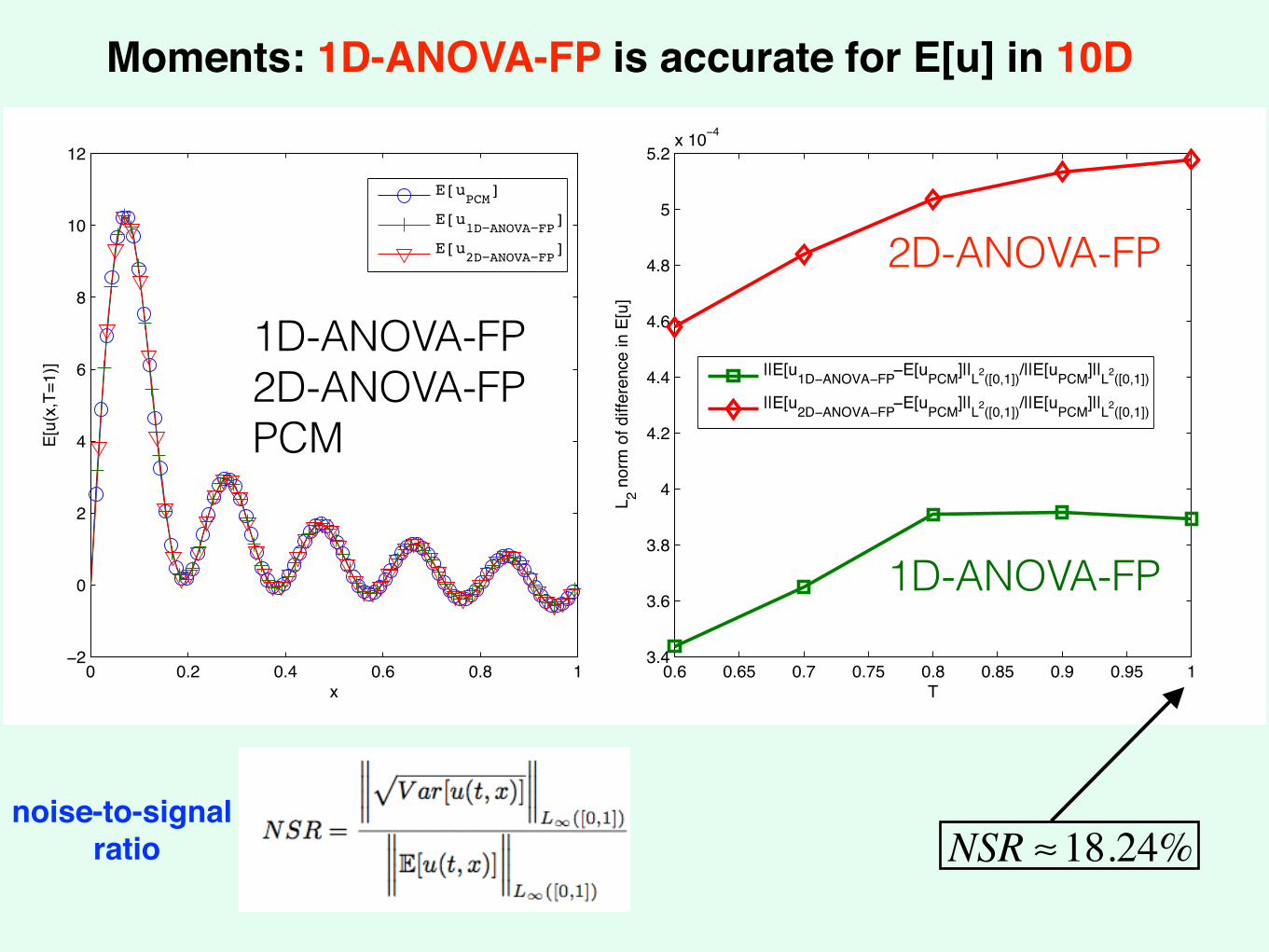
Moments: 1D-ANOVA-FP is accurate for E[u] in 10D
1D-ANOVA-FP 2D-ANOVA-FP PCM
1D-ANOVA-FP
2D-ANOVA-FP
noise-to-signal!ratio NSR ≈18.24%

Moments: 1D-ANOVA-FP is not accurate for in 10D
0 0.2 0.4 0.6 0.8 10
20
40
60
80
100
120
x
E[u
2 (x,T
=1)]
E[u2PCM]
E[u21D−ANOVA−FP]
E[u22D−ANOVA−FP]
0.6 0.65 0.7 0.75 0.8 0.85 0.9 0.95 10
0.05
0.1
0.15
0.2
0.25
0.3
0.35
0.4
T
L 2 nor
m o
f diff
eren
ce in
E[u
2 ]
||E[u21D−ANOVA−FP−E[u2
PCM]||L2([0,1])/||E[u2PCM]||L2([0,1])
||E[u22D−ANOVA−FP−E[u2
PCM]||L2([0,1])/||E[u2PCM]||L2([0,1])
1D-ANOVA-FP 2D-ANOVA-FP PCM
1D-ANOVA-FP
2D-ANOVA-FP
Ε[u2 ]
NSR ≈18.24%

Moments: PCM vs. FP (TFPDE)
Initial condition of FP equation introduce error
0.2 0.4 0.6 0.8 110−10
10−8
10−6
10−4
10−2
l2u2
(t)
t
PCM/S Q=5, q=2PCM/S Q=10, q=2TFPDE
NSR 5 4.8%
Moments: PCM vs. MC
LePage’s representation (2D)
Ε[u2 ]
Ε[u2 ]LePage’s representation (2D)
100 102 104 10610−4
10−3
10−2
10−1
s
l2u2
(t=1)
PCM/S q=1PCM/S q=2MC/S Q=40
PCM costs less than MC
Q — # of truncation in series representation q — # of quadrature points on each dimension

Density: MC vs. FP equation (2D Levy) LePage’s !representation!2D — MC 3D — FP
Levy!copula
t = 1
t = 1
t = 1.5
t = 1.5

General picture of solving SPDEs w/ multi-dim jump processes

Summary of contributions (3, 4)✰ Established a framework for UQ of SPDEs w/ multi-
dimensional Levy jump processes by probabilistic (MC, PCM) and deterministic (FP) methods
✰ Combined the ANOVA & FP to simulate moments of solution at lower orders
✰ Improved the traditional MC method’s efficiency and accuracy
✰ Link the area of fractional PDEs & UQ for SPDEs w/ Levy jump processes

Outline ♚ Adaptive multi-element polynomial chaos with discrete
measure: Algorithms and applications to SPDEs
♚ Adaptive Wick-Malliavin (WM) approximation to nonlinear
SPDEs with discrete RVs
♚ Numerical methods for SPDEs with 1D tempered -stable (T S) processes
♚ Numerical methods for SPDEs with additive multi-dimensional Levy jump processes
♚ Future work
αα

Future work For methodology:!✰ Simulate SPDEs driven by higher-dimensional Levy jump processes
with ANOVA-FP ✰ Consider other jump processes than TS processes ✰ Consider nonlinear SPDEs w/ multiplicative multi-dimensional Levy
jump processes !For applications:!✰ Application to the Energy Balance Model in climate modeling: P.
Imkeller, Energy balance models - viewed from stochastic dynamics, Stochastic climate models, Basel: Birkhuser. Prog. Probab., 49 (2001), pp. 213– 240.
!✰ Application to Mathematical Finance such as the stock price model
associated with multi-dimensional Levy jump processes: R. Cont, P. Tankov, Financial Modelling with Jump Processes, Chapman & Hall/CRC Press, 2004.

Acknowledgements✰ Thanks Prof. George Em Karniadakis for advice and
support ✰ Thanks Prof. Xiaoliang Wan and Prof. Hui Wang to be on
my committee ✰ Thanks Prof. Xiaoliang Wan and Prof. Boris Rozovskii for
their innovative ideas and collaboration ✰ Thanks for the support from the National Science
Foundation, "Overcoming the Bottlenecks in Polynomial chaos: Algorithms and Applications to Systems Biology and Fluid Mechanics" (Grant #526859)
✰ Thanks for the support from the Air Force Office of Scientific Research: Multidisciplinary Research Program of the University Research Initiative, "Multi-scale Fusion of Information for Uncertainty Quantification and Management in Large-Scale Simulations" (Grant #521024)

Thanks for attending !


