draft, march 1, 2007
TRANSCRIPT
draft, March 1, 2007
Numerical simulations of rarefied gases in curved channels:
thermal creep, circulating flow, and pumping effect
Kazuo Aoki1, Pierre Degond2, Luc Mieussens2
Abstract. We present numerical simulations of a new system of micro-pump basedon the thermal creep effect described by the kinetic theory of gases. This device is madeof a simple smooth and curved channel along which is applied a periodic temperature field.Using the Boltzmann-BGK model as the governing equation for the gas flow, we develop anew numerical method based on a deterministic finite volume scheme, implicit in time, withan implicit treatment of the boundary conditions. This method is comparatively faster thanthe usual Direct Simulation Monte Carlo method in case of long devices, and turns to beaccurate enough to compute macroscopic quantities like the pressure field in the channel.Our simulations show the ability of the device to produce a one-way flow that has a pumpingeffect.
Key words. Knudsen compressor, thermal creep flow, transpiration flow, BGK model,implicit scheme
AMS subject classifications. 76P05, 82B40, 82D05, 82C80, 65M06
1 Introduction
In the vicinity of solid boundaries, flows of rarefied gases show a large variety of phenomenathat do not exist for dense gases as described by continuous gas dynamics (like Stokes orNavier-Stokes equations). For instance, several effects due to a temperature field applied on asolid boundary have been observed that cannot be explained in the framework of classical gasdynamics: let us mention thermal stress slip flow, nonlinear thermal stress flow, flow inducednear a heated plate edge, thermophoresis, and thermal creep flow (see Sone [34, 35, 36]). Thislast phenomenon was already described (as thermal transpiration) by Reynolds in 1879 [31]:in a rarefied gas contained in a pipe whose temperature has a gradient along its axis, a
1Department of Mechanical Engineering and Science, Graduate School of Engineering, Kyoto University,Kyoto 606-8501, Japan
2Institut de Mathmatiques de Toulouse (UMR 5219), Universite Paul Sabatier, 118, Route de Narbonne,31062 TOULOUSE cedex 9, France ([email protected], [email protected]) This re-search was supported partially by the joint research project between JSPS and CNRS “Projet Internationalde Coopration Scientifique (PICS)” of CNRS, grant n. 3195; computational resources have been providedby the CALMIP project (Calcul en Midi-Pyrenees), University Paul Sabatier, Toulouse, France
1

flow is induced in the direction of the gradient, and this flow has a pumping effect, whilethe device does not involve any moving part or mixing process. Recently, interest in thiskind of flows is growing in connection with micro machine engineering, like Micro-Electro-Mechanical Systems (see Karniadakis, Beskok and Aluru [18] and Cercignani [12]). Indeed,the thermal creep is observed only if the gas is rarefied, that is to say when the characteristiclength scale of the device containing the gas is not large with respect to its mean free path.This implies that one needs to use either very low pressure conditions, or a very small device.Different systems have recently been proposed to design pumping systems using this effect(see for instance Pham-Van-Diep et al. [29], Sone, Waniguchi and Aoki [41], Aoki et al [4],Vargo and Muntz [44]). They are often called Knudsen compressors since Knudsen himselfin 1909 [19] described the first experimental device of this kind. The basic idea is to usecascade systems whose single unit is a pipe composed of a thin part connected to a thickerpart. With two opposed temperature gradients applied to each part of the unit (so as thereis no temperature gradient on the average), two opposed thermal creep flows are created,one of whom being stronger than the other one due to a geometric effect. A one-way flowcan then be generated in the whole unit without applying any pressure gradient externally.This flow has a pumping effect that can be amplified by connecting several units to form acascade system.
In this paper, we consider a new simple device in which the thermal creep flow is createdby using a simple curved channel on which is applied a periodic temperature field. Asopposed to [41], we do not use any complex connection part. Up to our knowledge, such adevice has never been presented before. Since any experimental study of such micro-systemsis a difficult challenge, our aim is here to use numerical simulations to demonstrate that ourdevice can effectively produce a one-way flow. We also want to prove that there exists apumping effect in the corresponding cascade system, which means that it is indeed a Knudsencompressor. However, large numerical simulations of rarefied gas problems are still a delicateissue, since this always implies using a large number of degrees of freedom. Indeed, even fortwo-dimensional plane flows, the distribution function of the particle velocities of the gashas six independent variables.
For that purpose, we propose a new fast deterministic numerical method to accuratelysimulate rarefied gas flows. Actually, the most used numerical method for rarefied gasesis the direct simulation Monte-Carlo method (DSMC) proposed by Bird [8]. It is a veryrobust and efficient method, now very well understood, in which complex physics can beincluded. However it remains that this method is intrinsically an unsteady method in whichthe numerical time scale must be smaller than the physical time scale to compute the flowwith enough accuracy. This makes the DSMC method sometimes difficult to use when oneis interested in computing slow flows for which the steady state is reached after very longtransients (even if new Monte Carlo methods like the Time Relaxed Monte Carlo of Pareschiand Russo [28] have recently been proposed that are free of such constraint). In such cases,the computational time needed to accurately capture the steady solution can be huge (seean example in section 5.4). Nevertheless, it has already been shown in [41, 4] that DSMCcan be used in the context of Knudsen compressors.
2

There also exist deterministic methods that use finite difference approximations of theBoltzmann equation. We mention for instance the works of Rogier and Schneider [32],Buet [10], or the works of Aristov and collaborators cited in [5]. Recently, for some simpleinteraction potentials, fast approximations of the Boltzmann collision operator have been pro-posed that considerably reduce its computational complexity (see Bobylev and Rjasanow [9],Filbet, Mouhot and Pareschi [14]). However, all these methods generally make use of thesame splitting strategy between collision and transport process (as in the DSMC method).This technique suffers from severe time step restrictions that can be prohibitive for steadystate calculations. Up to our knowledge, there are few methods for which the steady Boltz-mann equation is directly solved. We mention the works of Ohwada [26] and Sone andTakata [40] in which a very accurate discretization accounts for possible discontinuities ofthe distribution function. However, these methods are restricted to very simple geometries,in particular due to their marching-in-space algorithm.
Here we propose a different approach in which we apply classical computational fluid dy-namics tools to the kinetic framework. First we consider the simpler Bathnagar-Gross-Krook(BGK) model of the Boltzmann equation. While this simplification is not physically welljustified, it allows to easily reduce the computational complexities of collisions. Moreover,it is useful to obtain qualitative informations on a rarefied flow, and it is known to giveaccurate results in some situations [15]. Then we discretize the unsteady BGK equation intwo dimensional (2D) plane geometries by a finite volume scheme using structured mesheson arbitrary curvilinear grids. The steady state is rapidly reached by using a linearized timeimplicit scheme. This implicit time discretization can be viewed as a compromise betweena direct solving of the steady equation by a Newton-Raphson procedure and an unsteadycomputation. It allows to take very large time steps without stability problems. With thelinearization procedure, the use of expensive algebraic nonlinear solvers is avoided. More-over, as it is classical in numerics for kinetic equations, we use a robust velocity discretizationof the collision operator that preserves the physical properties of conservation and entropy.Our approach is an extension of a method developed by one of the authors in [23, 24] forwhich we propose two major modifications: first, due to the simple structure of the 2D planeBGK equation, we are able to use the reduced distribution technique [16] to remove the de-pendency of the distribution function on the third component of the particle velocity. Thisreduces the number of dimensions of the problem from 5 to 4. Second, we propose a newimplicit time discretization of the boundary conditions in order to speed up the convergenceof our algorithm towards steady state. The difficulty of such treatment is that the discretizedconvection operator is much more complicated: the boundary conditions introduce non localterms both in space positions and velocities. Usually, these terms are set to 0 by using anexplicit time discretization of the boundary conditions, but this is observed to give a poorlyconvergent algorithm, in particular in the present case of long cascade systems. Here, weintroduce a simple implicit treatment that naturally makes use of the iterative linear solverused in the scheme. This modification considerably speeds up the algorithm for some partic-ularly long computations. This numerical method has been implemented in a parallel codewhich turns out to be very robust and flexible enough to treat various gas kinetic simulation
3
problems.This method is then used to investigate the ability of our device to generate circulating
flows and pumping effects. The accuracy of our computation reveals the complex structureof the flow in our device. We also investigate the pumping effect obtained with a variousnumber of units in our cascade system. Although DSMC computations in such cases arevery heavy, we make several comparisons between this method and our deterministic resultsthat demonstrate both the accuracy of our approach as well as its performance in terms ofcomputational time.
The outline of this paper is the following. In section 2, we briefly give some elements ofkinetic theory needed to present our method, and we give some details on the thermal creepflow mechanism. In section 3, a rapid review of previous Knudsen compressors is presented,and our new device is detailed. The numerical method is presented in section 4, while somedetails are left to appendices A and B. Finally, we present our simulation results in section 5.
2 Rarefied gases and thermal creep flow
2.1 Kinetic description of a rarefied gas
In kinetic theory, a monoatomic gas is described by the distribution function F (t,x,v)defined such as F (t,x,v)dxdv is the mass of molecules that at time t are located in anelementary space volume dx centered in x = (x, y, z) and have a velocity in an elementaryvolume dv centered in v = (vx, vy, vz).
Consequently, the macroscopic quantities as mass density ρ, momentum ρu and totalenergy E are defined as the five first moments of F with respect to the velocity variable,namely:
(ρ(t,x), ρu(t,x), E(t,x)) =
∫
R3
(1,v,1
2|v|2)F (t,x,v) dv. (1)
The temperature T of the gas is defined by the relation E = 12ρ|u|2 + 3
2ρRT , where R is the
gas constant defined as the ratio between the Boltzmann constant and the molecular massof the gas.
When the gas is in a thermodynamical equilibrium state, it is well known that the dis-tribution function F is a Gaussian function M[ρ,u, T ] of v, called Maxwellian distribution,that depends only on the macroscopic quantities as
M[ρ,u, T ] =ρ
(2πRT )3
2
exp(−|v − u|22RT
). (2)
It can easily be checked that M satisfies relations (1).If the gas is not in a thermodynamical equilibrium state, its evolution is described by the
following kinetic equation∂tF + v · ∇xF = Q(F ), (3)
4
where the left-hand side describes the transport of molecules along straight lines, whilethe right-hand side describes the effect of collisions between molecules. The most realisticcollision model is the Boltzmann operator but it is still very computationally expensive touse. In this paper, we prefer to use the simpler BGK model [6, 46]
Q(F ) =1
τ(M[ρ,u, T ] − F ) (4)
which models the effect of the collisions as a relaxation of F towards the local equilibriumcorresponding to the macroscopic quantities defined by (1). The relaxation time is definedas τ = µ
ρRT, where µ is the viscosity of the gas. It is usually supposed to fit the following
law µ = µref(T
Tref)ω, where µref and Tref are reference viscosity and temperature determined
experimentally for each gas, as well as the exponent ω (see a table in [8]). In this paper,we shall use the simplest law obtained with ω = 1. This corresponds to the viscosity lawobtained with the Boltzmann equation for Maxwellian molecules [11].
2.2 Interaction with the boundaries
Modeling gas-surface interactions is an important problem, still the subject of current re-searches. In this work, we shall use the classical and simple diffuse reflection model. Theinfluence of other interaction models on the results presented in this paper is deferred to afuture work.
In the diffuse reflection model, the boundary is supposed to have a velocity uw andtemperature Tw. A molecule that collides with this boundary is supposed to be re-emittedwith a temperature equal to Tw, and with a random velocity normally distributed arounduw. This reads
F (t,x,v) = σM[1,uw, Tw](v) (5)
if v · n(x) > 0, where n(x) is the normal to the wall at point x directed into the gas.The parameter σ is defined so as there is no normal mass flux across the boundary (all themolecules are re-emitted). Namely
σ = −(
∫
v·n(x)<0
F (t,x,v)v · n(x) dv
)
/
(∫
v·n(x)>0
M[1,uw, Tw](v)v · n(x) dv
)
. (6)
2.3 Thermal creep flow
The thermal creep is a boundary effect that exists only for slightly rarefied gases. Considera gas close to a boundary along which is applied a temperature gradient, to say a lowtemperature on the left and a high temperature on the right. If the gas is rarefied enough,the temperature gradient generates a gas flow from the left to the right (that is from thelow to the high temperature). At the contrary, this effect does not appear if the gas is in acontinuous (dense) regime.
5
This phenomenon has been known for a long time, as for instance in the particular caseof a gas contained in a pipe or a channel where the walls are heated along with a temperaturegradient: this “thermal transpiration” has been first discovered by Reynolds in 1879 [31, 30]who proposed both experimental and theoretical studies of this phenomenon. Using thework of Reynolds, Maxwell proposed another theoretical analysis in [22]. Later, this wasalso the subject of a work by Knudsen [19, 20]. However, this is much more recently that acomplete and accurate analysis on the basis of the Boltzmann equation has been proposedby Sone [33] (see also Ohwada, Sone and Aoki [27]). Very recently, a continuous theory ofthis phenomenon has been proposed by Bielenberg and Brenner [7].
Without describing these theories in details, we only give below a simple explanation(taken from [35]) of the thermal creep physical mechanism. Consider a point A of theboundary (see figure 1) and the molecules that impact this point. Since the boundary ishotter at the right of A than at the left, then the molecules coming from the right have agreater average kinetic energy than those coming from the left. Consequently these moleculestransfer a momentum to A which is greater than the momentum transfered by left molecules.On the other hand, the molecules reflected diffusely on the boundary do not contribute to thetangential momentum transfer. Therefore the gas transfers a momentum to the boundaryin the opposite direction to the temperature gradient direction (to say from the right tothe left). Finally, since the boundary is at rest, by reaction it transfers a force to the gasdirected from the left to the right. This produces a flow directed in the temperature gradientdirection. This flow is called thermal creep flow. Note that this phenomenon disappears inthe continuous (dense) regime.
This effect suggests that it is possible to create a gas flow without any mechanical part.This has been studied for a long time (see the numerous references given in [35], section3.11.6). Several experimental studies have clearly demonstrated the practical possibility touse this phenomenon to create a pumping system (see section 3.1).
Since the thermal creep is generated only when the gas is “slightly rarefied”, this meansthat the size of such pumping systems should not be too large with respect to the mean freepath of the gas. For instance, for the air at atmospheric pressure, the characteristic size ofthe device should be of the order of 0.1 microns. This is why recently, due to advances inmicro-fabrication, there has been a renewed interest in applications of the thermal creep inthe context of Micro-Electro-Mechanical Systems (MEMS) [41, 17, 45, 44].
In the following sections, we describe the pumping effect induced by the thermal creepflow, as well as some devices designed to use this effect.
3 Pumping systems using the thermal creep
3.1 Pumping effect and Knudsen compressors
The first application of the thermal creep phenomenon to design pumps without any me-chanical part is due to Knudsen [19, 20]. The basic idea of this system is the following: whentwo reservoirs are joined by a pipe with a temperature gradient, classical fluid mechanics
6

predicts that at steady state the pressure is constant in the device. But if the pipe is thinenough, so that the gas contained in the pipe is slightly rarefied, then a thermal creep flowis generated by the temperature gradient in the direction of this gradient. A small amountof gas is then pumped out of the reservoir of lower temperature and sent into the reservoirof higher temperature. This creates a small pressure difference between the two reservoirs,which is called the pumping effect.
However, this pressure difference is very small. It can be increased by using a largertemperature gradient, but of course, this gradient cannot be increased indefinitely. Knudsensuggested to use a cascade system in which a basic unit is composed of a pipe with atemperature gradient connected to a section with an opposed temperature gradient so thatthe two ends of the unit are kept at the same temperature. Of course, these two gradientscreate two opposed thermal creep flows. The pipe and the connecting section must bedesigned so that these flows do not cancel each other, and it is hoped that a global massflow will be generated.
Before the recent development of micro-mechanics, it was not possible to build sufficientlysmall systems, so much so that the rarefied gas conditions needed to produce a thermal creepmake necessary to use very low pressures. This is why this system was not intensively studieduntil a recent period. With the growing of MEMS technology, several modern versions ofthe Knudsen compressor have been proposed. For instance [29] and [44] studied the pressuredifference obtained with a Knudsen compressor in which capillary pipes are obtained byusing a thin membrane. Another strategy (without membrane) was proposed by [41] and [4]who used a cascade system of channels or pipes with a periodic temperature. A basic unitis composed of a pipe with an increasing temperature in the first part, and a decreasingtemperature in the second part. The opposit thermal creep of the second part is maintainedin a recirculation flow in a ditch dug along the pipe. Then a global mass flow due to thethermal creep of the first part is generated in the unit. A pumping effect is also observed inthe case of a system closed at both ends. This has been investigated both numerically andexperimentally in [41, 4, 38].
Using this last idea, we present in the following section a new device that could be usedas a Knudsen compressor.
3.2 A new device using curved channels
While the previous systems have been proved to be very efficient, their geometrical structureis not very simple. In particular, this seems difficult to use them for small systems as MEMS.Instead of using ditches to apply a temperature gradient, we propose to use curved parts ofa smooth channel. This should be much simpler to realize on MEMS.
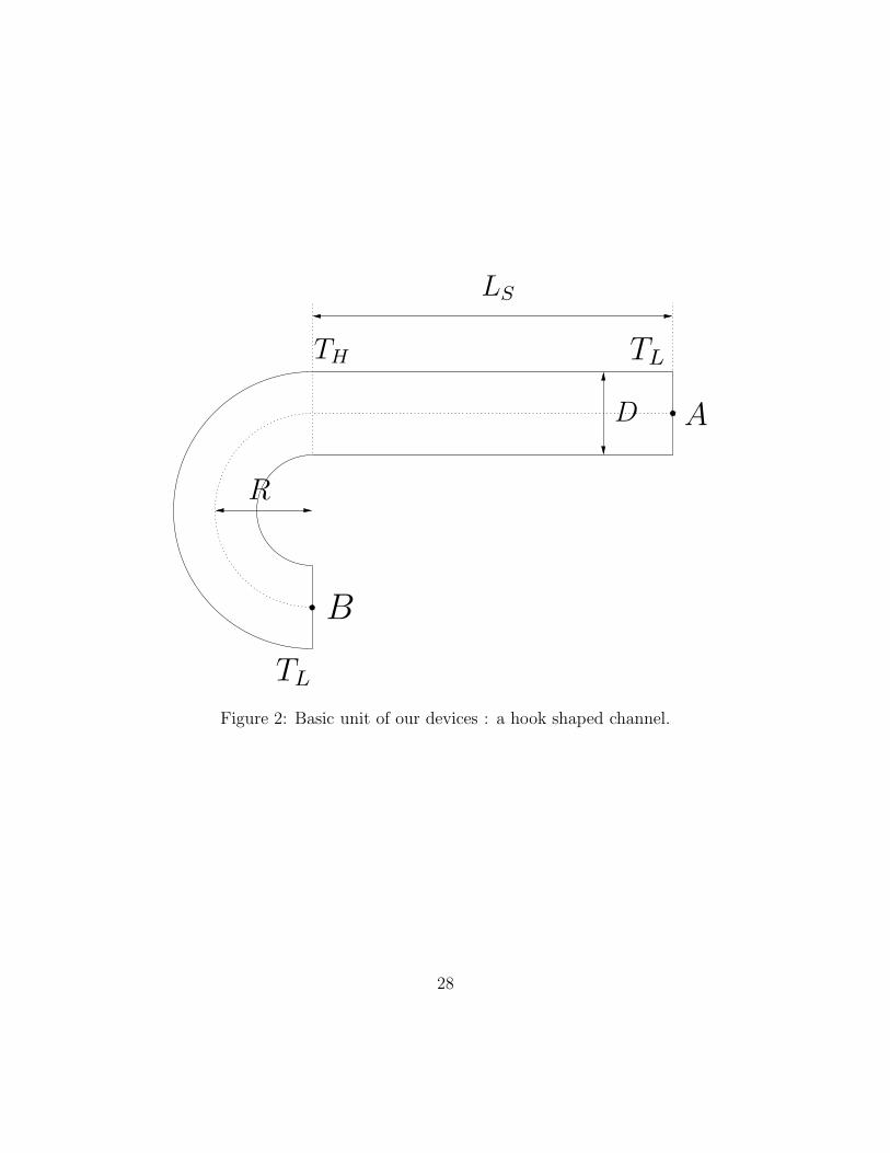
Basically a single unit of our device is detailed in figure 2. It has a hook shape thatis composed of a straight channel joined to a circular curved part. A uniform temperaturegradient is applied to the straight part (the temperature increases linearly from TL to TH
along the channel), while an opposed temperature gradient is applied to the curved part.For some reasons as explained in section 3.1, it is expected that two opposed thermal creep
7

flows will be generated in the different parts. Due to the different geometries of these parts,one can hope that one of these flows should be stronger than the other one. Then a globalnet flow should be created.
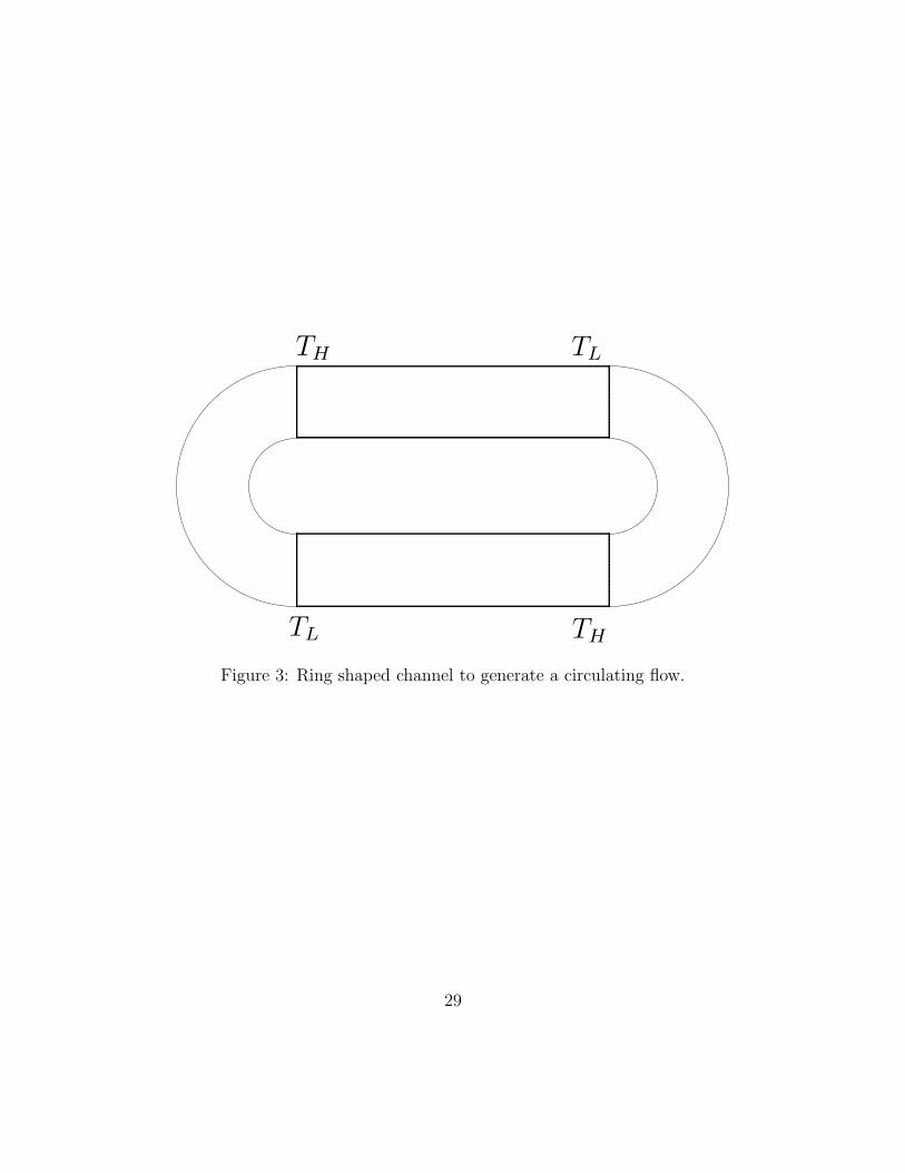
Consequently, the first test we propose is to generate a circulating flow by joining oneunit and its symmetric image to form a ring as described in figure 3.
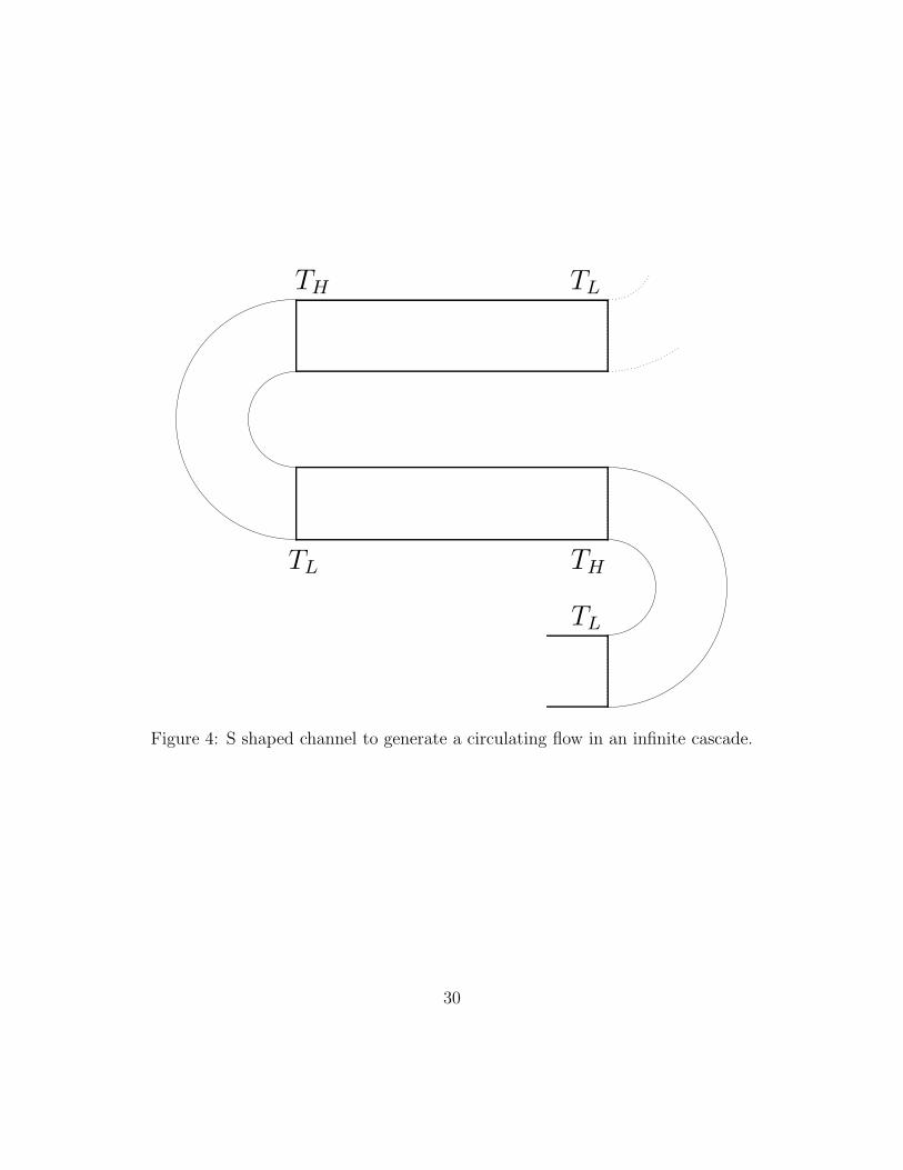
A similar test consists in joining one unit to its symmetric mirror image to form a S shape(see figure 4). Then periodic boundary conditions can be applied to both ends to generatean infinite cascade of S shapes.
Note that these two tests can be simulated by using only one unit as in figure 2 andappropriate “periodic” boundary conditions at both ends (see below).
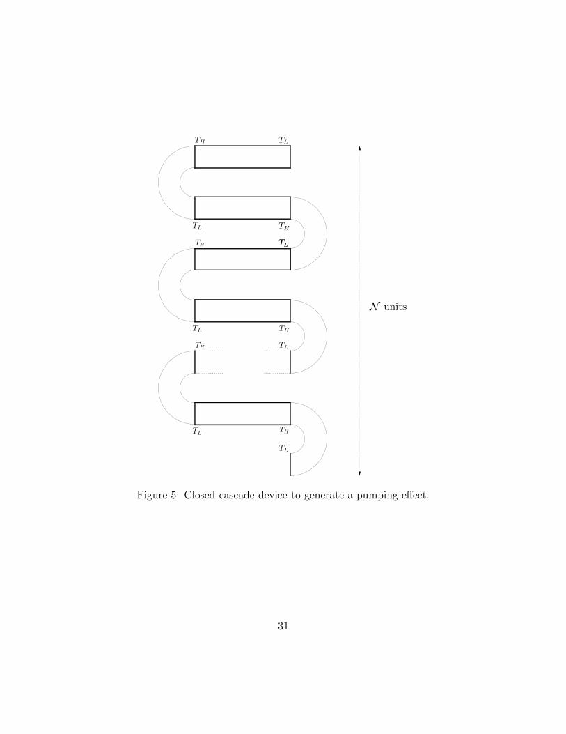
The second test we propose is similar to the previous cascade system, except that weuse a finite number N of units as described in figure 5. Moreover, this system is closed atboth ends to create a pumping effect. Namely, we want to observe that pressure and densitydifferences can be maintained at steady state between the two ends.
It should be mentioned that we have investigated the same problem using the DSMCmethod and observed that the idea mentioned above actually works [1].
The boundary conditions we use are diffuse reflection on the straight and curved bound-aries (as detailed in section 2.2). For the circulating flow in the ring shape, we apply thefollowing symmetry periodic boundary conditions at both ends A and B of a single unit
F (t, A, vx, vy, vz) = F (t, B,−vx,−vy, vz). (7)
For the circulating flow in the infinite cascade of S shapes, we apply this different symmetryperiodic boundary condition
F (t, A, vx, vy, vz) = F (t, B,−vx, vy, vz). (8)
For the pumping system, the diffuse reflection condition is applied to both ends with the lowtemperature TL.
In the next sections, we detail our numerical method to solve the BGK equation inthese three different devices. However, note that for computational cost reasons, this studyis restricted to plane channels. To say, figures 3, 4, and 5 represent constant sections ofchannels that are infinite in the direction orthogonal to the figures. More realistic circularpipes would require full 3D computations, which is at present far from being reachable, inparticular with the third device in case of a large number of units.
4 Numerical method
4.1 Reduced BGK model
In case of plane flows, F is independent of z and hence the transport operator in (3) doesnot contain explicitly the velocity vz.
8

Consequently, the computational complexity of the BGK equation (3) can be reduced byusing the classical reduced distribution technique (first introduced—up to our knowledge—by Huang and Hwang for polyatomic gases in [16]). This approach is widely used to compute2D flows, see for instance [47, 3, 37]. For the sake of completeness, this method is rapidlydetailed below.
We define the reduced distribution functions
f(t, x, y, vx, vy) =
∫
R
F dvz,
g(t, x, y, vx, vy) =
∫
R
1
2v2
zF dvz.
Now we denote by v = (vx, vy) and x = (x, y) the 2-dimensional velocity and positionvariables. By symmetry the macroscopic velocity u has no component along z and we shalldenote accordingly by u = (ux, uy) its component in the plane (x, y). Then it is easy to showthat f and g solve the following coupled system of relaxation equations
∂tf + v · ∇xf =1
τ(M [ρ, u, T ] − f),
∂tg + v · ∇xg =1
τ(RT
2M [ρ, u, T ] − g),
(9)
where M [ρ, u, T ] is the reduced Maxwellian defined by
M [ρ, u, T ] =
∫
R
M[ρ,u, T ] dvz =ρ
2πRTexp(−|v − u|2
2RT),
and the macroscopic quantities are obtained through f and g by
ρ =
∫
R2
f dv,
ρu =
∫
R2
vf dv,
T =1
32ρR
∫
R2
(1
2|v − u|2f + g) dv.
(10)
With this procedure, the variable vz is eliminated. Consequently, system (9) is compu-tationally less expensive than (3).
Note that the reduced distributions f and g as well as the macroscopic quantities areindeed those of the full distribution F without any approximation. Once the macroscopicquantities are obtained, F can be reconstructed easily from the original equation (3) with (4)that is just a differential equation for F .
9
4.2 Velocity discretization
Here we propose a robust velocity discretization of (9). This approach is based on thework of Mieussens in [23, 24] (see also a similar extension for a reduced BGK model forpolyatomic gases in [13]). The main idea is to design a discretization of the Maxwelliandistribution M [ρ, u, T ] such that the discretized version of (9) satisfies the same propertiesas the continuous one, namely conservation and entropy properties. We refer to [25, 13] formathematical proofs of existence and consistency results for such approximations.
More precisely, we define a Cartesian grid V of Nv nodes vk = (vkx = a + k∆vx, v
ly =
b + l∆vy) where k = (k, l) is a couple of bounded indexes. We denote by fk and gk theapproximations of f(vk) and g(vk). The macroscopic quantities are now defined by using asimple rectangle quadrature as
ρ =∑
k
fk∆v,
ρu =∑
k
vkfk∆v,
E =1
2|u|2 +
3
2ρRT =
∑
k
(1
2|vk|2fk + gk)∆v,
(11)
where ∆v = ∆vx∆vy. For clarity, we now introduce the following 4-dimension vectors
~ρ = (ρ, ρu, E)T , ~m(v) = (1, v,1
2|v|2)T , ~e = (0, 0, 0, 1)T .
Then the previous relations (11) read in a very compact form
~ρ =∑
k
(~m(vk)fk + ~e gk) ∆v. (12)
These notations allow to simplify the writing of the velocity discretization of (9). Thisapproximation now is
∂tfk + vk · ∇xfk =1
τ(Mk[~ρ ] − fk),
∂tgk + vk · ∇xgk =1
τ(Nk[~ρ ] − gk),
(13)
where Mk[~ρ ] and Nk[~ρ ] are approximations of M [ρ, u, T ](vk) and RT2M [ρ, u, T ](vk) defined
to ensure that the discrete BGK system (13) satisfies the same properties of conservationand entropy as the continuous model (9). Namely we have
Mk[~ρ ] = exp(~α(~ρ )T ~m(vk)), Nk[~ρ ] = − 1
2α4(~ρ )Mk[~ρ ], (14)
10
where ~α = (α1, α2, α3, α4)T solves the following non linear 4 × 4 system
∑
k
~m(vk) exp(~α(~ρ )T ~m(vk))∆v − ρ
2α4(~ρ )~e = ~ρ. (15)
Note that in the continuous case (that is to say with integrals on R2 instead of quadratures),
we have an explicit relation between ~α(~ρ ) and ~ρ, namely
α(~ρ ) =
(
log( ρ
2πRT
)
− |u|22RT
,u
RT,− 1
RT
)T
. (16)
This relation is not valid in the discrete case, but it is used in our code to solve nonlinearsystem (15) by a Newton algorithm.
4.3 Linearized implicit scheme
Here we propose a time and space discretization of the system of the reduced discrete BGKequations (13).
Consider a spatial Cartesian grid defined by nodes (xi, yj) = (i∆x, j∆y) and cells ]xi− 1
2
, xi+ 1
2
[
×]yj− 1
2
, yj+ 1
2
[ for i = 1 to imax and j = 1 to jmax. The number of cells is denoted byNc = imaxjmax. Consider also a time discretization with tn = n∆t. If fn
k,i,j and gnk,i,j are
approximations of fk(tn, xi, yj) and gk(tn, xi, yj), the moments ~ρ defined by (12) are naturallyapproximated by
~ρni,j =
∑
k
(~m(vk)fnk,i,j + ~egn
k,i,j) ∆v.
The transport part of (13) is approximated by a standard finite volume scheme. For thenonlinear relaxation term, a standard centered approximation technique is used. Our schemethus reads
fn+1k,i,j = fn
k,i,j − ∆t
∆x
(
Fi+ 1
2,j(f
nk ) − Fi− 1
2,j(f
nk )
)
− ∆t
∆y
(
Fi,j+ 1
2
(fnk ) −Fi,j− 1
2
(fnk )
)
+∆t
τni,j
(Mk[~ρni,j] − fn
k,i,j), (17)
gn+1k,i,j = gn
k,i,j − ∆t
∆x
(
Fi+ 1
2,j(g
nk ) −Fi− 1
2,j(g
nk )
)
− ∆t
∆y
(
Fi,j+ 1
2
(gnk ) − Fi,j− 1
2
(gnk )
)
+∆t
τni,j
(Nk[~ρni,j] − gn
k,i,j)
where the numerical fluxes are defined for every grid function {ϕk,i,j} by
Fi+ 1
2,j(ϕk) =
1
2
(
vkx(ϕk,i+1,j + ϕk,i,j) − |vk
x|(∆ϕk,i+ 1
2,j − Φn
k,i+ 1
2,j))
Fi,j+ 1
2
(ϕk) =1
2
(
vly(ϕk,i,j+1 + ϕk,i,j) − |vl
y|(∆ϕk,i,j+ 1
2
− Φnk,i,j+ 1
2
))
(18)
11
with the notation ∆ϕk,i+ 1
2,j = ϕk,i+1,j − ϕk,i,j, and the flux limiter function Φn
k,i+ 1
2,j
allows
to obtain a second order scheme. Note that according to section 4.2, the discrete equilibriaMk[~ρ
ni,j] and Nk[~ρ
ni,j] are defined for each cell (i, j) through relations (14) and (15) by using
~ρni,j instead of ~ρ in the formula.
When indexes i and j correspond to cells located at the boundaries of the domain, thereappear unknown values in the numerical fluxes, like fn
k,0,j , fnk,imax+1,j, f
nk,i,0, f
nk,i,jmax+1 for the
first order scheme. Corresponding cells (0, j), (imax + 1, j), (i, 0), (i, jmax + 1) are calledghost-cells. These values are classically defined according to the boundary conditions (B.Cfor short) specified for the problem. Here we consider two types of B.C: diffuse reflections,that are local in space but global in velocities, and symmetry periodic conditions, thatcouple two different cells and two symmetric velocities. For instance, incident molecules ina boundary cell of indexes (i, j = 1) are supposed to be re-emitted by the wall from a ghostcell of indexes (i, 0). This cell is the mirror cell of (i, 1) with respect to the wall. The diffusereflection (5) is then modeled by
(fnk,i,0, g
nk,i,0) = σi,1 (Mk[1, uw, Tw], Nk[1, uw, Tw]), vk · ni,1 > 0, (19)
where σi,1 is determined so as to avoid a mass flux across the wall, i.e. between cells (i, 0)and (i, 1). Relation (6) gives
σi,1 = −∑
vk·ni,1<0 vk · ni,1 fnk,i,1∆v
∑
vk·ni,1>0 vk · ni,1Mk[1, uw, Tw]∆v.
For the symmetry periodic B.C of the ring shaped channel, relation (7) gives
fnk,0,j = fn
k′,imax,j, (20)
where k′ is such that vk′ = −vk. Finally, the symmetry periodic B.C (8) for the infinitecascade of S shaped channel gives the same relation with now k′ such that vk′ = (−vk
x, vly).
This scheme can also be written for curvilinear meshes as we did for the numericalsimulations of section 5. But to simplify the presentation, this is not presented here (see anexample for a single distribution BGK model in [24]).
Since this scheme is explicit, the CFL condition can be very restrictive, in particular forsteady state computations. A classical way to overcome this difficulty is to use an implicitscheme. It is derived from the explicit scheme by evaluating at tn+1 the transport andrelaxation terms responsible for stability problems with large ∆t. This scheme reads
fn+1k,i,j = fn
k,i,j − ∆t
∆x
(
Fi+ 1
2,j(f
n+1k ) − Fi− 1
2,j(f
n+1k )
)
− ∆t
∆y
(
Fi,j+ 1
2
(fn+1k ) − Fi,j− 1
2
(fn+1k )
)
+∆t
τni,j
(Mk[~ρn+1i,j ] − fn+1
k,i,j ), (21)
gn+1k,i,j = gn
k,i,j − ∆t
∆x
(
Fi+ 1
2,j(g
n+1k ) −Fi− 1
2,j(g
n+1k )
)
− ∆t
∆y
(
Fi,j+ 1
2
(gn+1k ) −Fi,j− 1
2
(gn+1k )
)
+∆t
τni,j
(Nk[~ρn+1i,j ] − gn+1
k,i,j)
12
The relaxation time is kept explicit, and for the second order scheme, the flux limiters(non differentiable) are kept explicit too. However this scheme is still nonlinear due to theequilibria Mk[~ρ
n+1i,j ] and Nk[~ρ
n+1i,j ]. As usual in hyperbolic implicit schemes, these terms are
linearized as follows
Mk[~ρn+1i,j ] ≈Mk[~ρ
ni,j] + ∂~ρMk[~ρ
n+1i,j ](~ρn+1
i,j − ~ρni,j),
Nk[~ρn+1i,j ] ≈ Nk[~ρ
ni,j] + ∂~ρNk[~ρ
n+1i,j ](~ρn+1
i,j − ~ρni,j),
where ∂~ρMk[~ρn+1i,j ] and ∂~ρNk[~ρ
n+1i,j ] are the Jacobian matrices of the mappings ~ρ 7→ Mk[~ρ ]
and ~ρ 7→ Nk[~ρ ]. See appendix A for detailed expressions of these Jacobian matrices.For implementation, it is useful to store all the unknowns into a single large 2-block
vector Un = (fn, gn), with blocks fn = {fnk }k and gn = {gn
k}k. The sub-blocks fnk and gn
k
are then stored as fnk = {fn
k,i,j}k,i,j and gnk = {gn
k,i,j}k,i,j. Then the linearized implicit schemeis rewritten under this δ matrix-form
(
I
∆t+ T +Rn
)
δUn = RHSn, (22)
where δUn = Un+1 − Un, I is the unit matrix, T is a matrix such that for every 2-blockvector V = (ϕ, ψ)
TV =
(
{ 1
∆x
(
Fi+ 1
2,j(ϕk) −Fi− 1
2,j(ϕk)
)
− 1
∆y
(
Fi,j+ 1
2
(ϕk) −Fi,j− 1
2
(ϕk))}
k,i,j
,{ 1
∆x
(
Fi+ 1
2,j(ψk) −Fi− 1
2,j(ψk)
)
− 1
∆y
(
Fi,j+ 1
2
(ψk) − Fi,j− 1
2
(ψk))}
k,i,j
) (23)
with only the first order fluxes. Moreover, the coefficient of T that would correspond tothe boundary conditions are classically set to 0. This corresponds to set δUn = 0, thatis to say fn+1 = fn and gn+1 = gn at these cells. This is called an explicit treatment ofthe boundary conditions, since at the contrary the right-hand side defined in (25) containsindeed the boundary terms. This considerably simplifies the structure of T since it is now adiscrete convection operator with homogeneous Dirichlet B.C (see below).
The relaxation matrix Rn is such that for every 2-block vector V = (ϕ, ψ)
RnV =
(
{ 1
τni,j
(ϕk,i,j − ∂~ρMk[~ρn+1i,j ]~ρ(Vi,j))
}
k,i,j,{ 1
τni,j
(ψk,i,j − ∂~ρNk[~ρn+1i,j ]~ρ(Vi,j))
}
k,i,j
)
,
(24)where we set ~ρ(Vi,j) =
∑
k(~m(vk)ϕk,i,j + ~eψk,i,j) ∆v. Finally, we set the right-hand side to
RHSn =
(
{
− 1
∆x
(
Fi+ 1
2,j(f
nk ) − Fi− 1
2,j(f
nk )
)
− 1
∆y
(
Fi,j+ 1
2
(fnk ) − Fi,j− 1
2
(fnk )
)
+1
τni,j
(Mk[~ρni,j] − fn
k,i,j)}
k,i,j
,{
− 1
∆x
(
Fi+ 1
2,j(g
nk ) − Fi− 1
2,j(g
nk )
)
− 1
∆y
(
Fi,j+ 1
2
(gnk ) − Fi,j− 1
2
(gnk )
)
+1
τni,j
(Nk[~ρni,j] − fn
k,i,j)}
k,i,j
)
,
(25)
13

which contains the limiters for the second-order scheme and the boundary conditions.It can be noted that relation (23) and (18) imply that T is a 2 × 2 block diagonal
matrix, in which each block of the diagonal is itself a Nv × Nv block diagonal matrix. Thesub-blocks—denoted by Tk—are Nc × Nc pentadiagonal matrices (see figure 6). Since therelaxation operator couples the velocities, but not the different space cells, the matrix Rn isa 2× 2 block matrix, in which the blocks are Nv ×Nv full block matrices. These sub-blocksare composed of Nc ×Nc diagonal matrices denoted by Rn
k,k′ on figure 6.The linear system (22) to be solved at each iteration is very large since its size is 2NvNc×
2NvNc. An iterative method well adapted to the different sparse structures of the matricesmay then be used. First, we extend the algorithm proposed in [24], which is based on acoupling between Jacobi and Gauss-Seidel methods. First, at the level of its small Nc ×Nc
sub-blocks, Rn is separated into its block diagonal ∆n and its block off-diagonal En, i.e.Rn = ∆n − En (this is the Jacobi step). Then system (22) is equivalent to
(
I
∆t+ T + ∆n
)
δUn = RHSn + EnδUn.
Since the matrix of this linear system is block diagonal with pentadiagonal blocks I∆t
+Tk+∆n
k (see figure 6), it is possible to use a line Gauss-Seidel method by setting Tk = Mk−Nk.This gives the following algorithm:
Algorithm 4.1. set V (0) = 0,for p = 0, . . . , P , solve
(
I
∆t+Mk + ∆n
k
)
V(p+1)k = RHSn
k +NkV(p)k + [EnV (p)]k, ∀k (26)
set δUn = V (P+1).
The linear systems (26) may easily and exactly be solved by successive LU decompositionsof tridiagonal matrices of R
imax×imax or Rjmax×jmax. Note that we do not need to store nor to
form the different matrices. Indeed, we only have to compute the coefficients of the diagonalblocks ∆n
k of Rn (see appendix B for a detailed expression). The matrix-vector products ofthe right-hand side of (26) are just the results of formula similar to (23) and (24).
While the number of iterations of the linear solver may be very large to reach convergenceto the exact solution, we only use a small number P ≤ 8. This is sufficient for the globalalgorithm to reach steady state.
In fact, we explain in the following section how we propose to modify this linear solverto improve the speed of convergence by taking into account the boundary conditions moreaccurately.
4.4 Implicit boundary conditions
It is observed in some cases that the convergence of our algorithm is quite slow, in particularfor long channels. Therefore it is natural to try to improve the treatment of the B.C so asto speed up this convergence.
14

In this section, we propose a simple implicit treatment of the B.C. The problem offully implicit B.C is that it deteriorates the simple block structure of the transport matrixT . Indeed, the diffuse reflection introduces a coupling between different velocities and thesymmetry periodic conditions introduce a coupling between very distant cells, as this can beseen in (19) and (20).
Consequently, for implicit boundary conditions, T is replaced in scheme (22) by thematrix T +B where T is untouched and B contains all the boundary terms. We find
(
I
∆t+ T +B +Rn
)
δUn = RHSn, (27)
Now, our linear solver 4.1 is simply modified by putting the matrix B in the right-hand sideto obtain
Algorithm 4.2. set V (0) = 0,for p = 0, . . . , P , solve
(
I
∆t+Mk + ∆n
k
)
V(p+1)k = RHSn
k +NkV(p)k + [EnV (p)]k − [BV (p)]k, ∀k (28)
set δUn = V (P+1).
Note that B is very sparse, even much sparser that T and Rn: it has at most 4(imax +jmax)Nv non-zero coefficients. Therefore, the additional cost of each iteration of this algo-rithm is very small, while we have observed that this simple modification speeds up theconvergence of the global method to steady state.
5 Numerical simulations
5.1 Parameters of the simulations
The circulating flow problem is characterized by four parameters. The two geometric onesare κ = D
Rthat measures the ratio between the width of the channel to the radius of the
circular part and B = LS
LS+πRwhich is the ratio between the length of the straight pipe to
the total length of one unit (see figure 2). The two physical parameters are the temperatureratio TH
TLand the Knudsen number
Kn =l0D
=
√2RTL
Dρ0RTref/µref
(29)
where l0 is the mean free path of the molecules at the equilibrium state at rest (ρ0 is theglobal average density in the channel).
The pumping problem is characterized by these parameters and the number N of ele-mentary units.
15

In the simulations presented here, only the parameters κ, Kn and N will vary. Thetemperature ratio TH
TLis set to 3 and the length ratio B is set to 0.5.
The gas we use is argon of molecular mass 0.663 10−20 kg, the initial velocity of the gasis zero, the low temperature TL is set to 300 K, and consequently the high temperature TH
is set to 900 K.The second order linearized implicit scheme is used in all the computations, with a CFL
number of 1000 (i.e. ∆t is 1000 times the explicit time step). The criterion used to determinewhether the flow has reached steady state is the reduction of the quadratic global residual1
∆t(∑
k,i,j |RHSnk,i,j|2)
1
2 by a factor of 105.The space domain is discretized by a curvilinear mesh with a uniform distribution of
nodes on the boundaries. The number of mesh cells depend on the test case.Note that the velocity grid is appropriately chosen for each case. Since the same grid
is used in each point of space, it should be large and precise enough to correctly describethe flow (i.e. the distributions everywhere in the space domain). The bounds are givenby a combination between the maximum macroscopic velocity and temperature of the flow(maxx(u + c
√RT ), where we take c = 4). The step of the grid is given by the smallest
temperature (i.e. ∆v = minx
√RT ). These quantities are estimated here by the data,
e.g velocity and temperature of the walls. Therefore, the velocity space is bounded to[−vmax, vmax]
3 with vmax = 1731 m.s−1. The velocity grid is then a regular Cartesian gridwith 40 points in vx and vy directions.
Finally, note that all the tests presented here have been computed on the SGI Altix 3700of the scientific grouping CALMIP (see http://www.calmip.cict.fr ). The algorithmpresented in section 4 has been implemented by L. Mieussens in a code called CORBIS (COdeRarefie Bidimensionel Implicite Stationnaire) by using the language Fortran 90 and theshared memory parallel programming interface OpenMP. The user time for all the differentsimulations was between two hours for the smallest case to 300 hours for the largest one(pumping effect with 16 units). Generally, we only used six processors for the simulations.
5.2 Circulating flow
5.2.1 Ring-shaped channel
We first test the ring-shaped device described in figure 3, for which one unit as describedin figure 2 is connected to its symmetric image. Due to this symmetry, the flow can besimulated in a single unit only, by using appropriate boundary conditions at the ends of theunit (see section 3.2).
We compute the steady flow for three different sizes of channel: thick (κ = 1), medium(κ = 0.5), thin (κ = 0.1), and for three different Knudsen numbers: Kn = 1, 0.5, 0.1. Thechannel is discretized with a number of cells that depends on its size: for the thick, medium,and thin channels we use respectively 400 × 96, 400 × 48, and 1600 × 24 cells. The firstnumber is the number of cells along the curvilinear direction parallel to the boundary of thechannel, and the second one is the number of cells along the orthogonal direction. Thesegrids have been chosen according to an accuracy study given at the end of this section.
16

In figures 7-15, we plot the non-dimensional velocity field u√2RTL
obtained at steady state
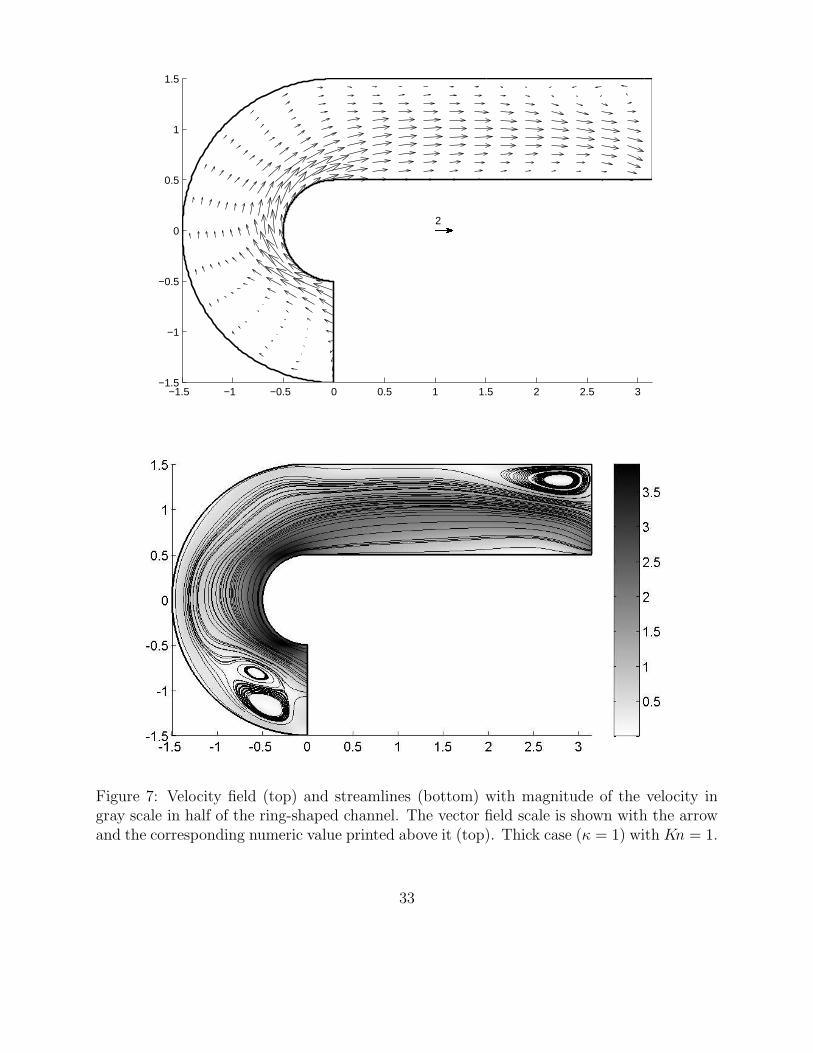
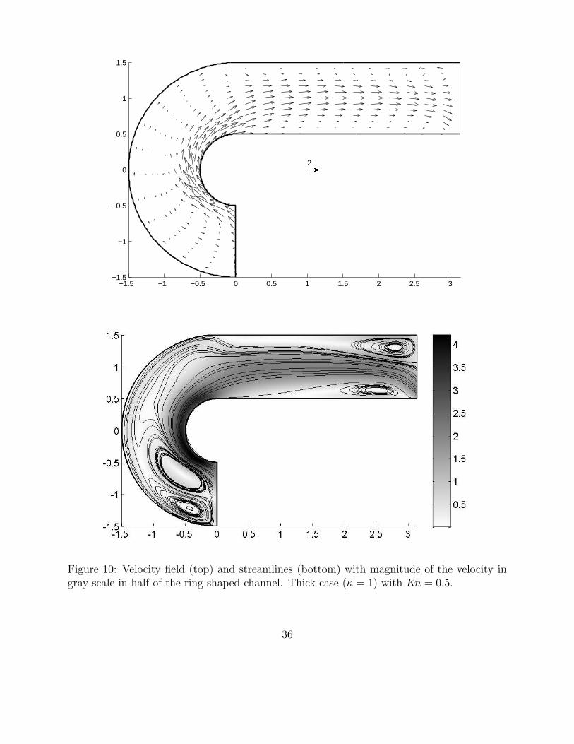
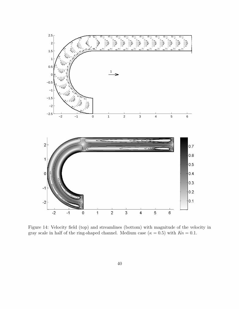
(top plot). Except for the thin channel, we also show a few streamlines plotted with themagnitude of the velocity field in gray scale (bottom plots of figures 7, 8, 10, 11, 13, 14).This allows to clearly see the movement of the gas. It appears that a circulating flow iswell generated, at least for Knudsen numbers Kn = 1 and 0.5 (see figures 7-12). The flowcirculates in the direction of the temperature gradient of the circular part, and is thereforeopposed to the direction of the temperature gradient of the straight part. This means thatthe thermal creep flow generated by the circular part is stronger than that created by thestraight part. This last one remains confined close to the straight boundaries, while themain flow created by the circular part propagates in the whole channel. This is probablydue to the curvature effect that increases the flow produced by the inner curved boundaryand at the same time gives rise to a higher resistance for the pressure-driven flow in thecurved channel. To sum up, the straight part plays the same role as the ditches of the devicestudied in [4, 41].
However the flow is far from being uniform in the channel. We can observe at least threerecirculation zones : two at the beginning of the circular part, and the other one at the endof the straight part. The velocities in these zones are very weak , but they are also strongeras κ decreases (the channel becomes thiner and longer). This can be seen on the top plotswith the velocity scale, and in the bottom plots with the magnitude of the velocity field infigures 7-12.
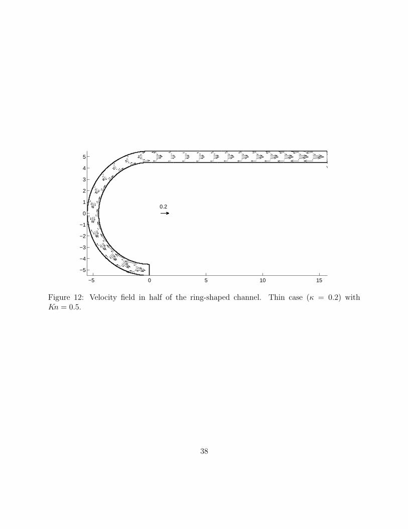
Finally, for the smallest Knudsen number Kn = 0.1 it is not clear wether a global massflow is really created along the channel. In figure 13 (thick case) there are very large recir-culation zones, and in figures 13-15 (thick, medium and thin cases) the thermal creep flowgenerated by the straight part looks as strong as the one of the circular part. However, it canbe noticed that the maximum velocities are still located close to the inner circular boundary.
Consequently, it seems more reliable to compute the average mass flow rate across asection of the channel to determine if there is or not a net mass flow created by our devices.Following [41, 4], we define the non-dimensionalized mass flow rate across a section Σ of thechannel by
M =
∫
Σρu · n dΣ
ρav
√2RTLD
,
where ρav is the average density in the channel. According to equations (3) or (9), thisquantity must be constant along the channel. However, due to numerical errors, it presentssome small fluctuations. Therefore, we compute an average of M along the channel, aswell as its standard deviation from this average (this also gives a good accuracy test for ourmethod). The results are plotted in figure 16 for the three different channels and for thethree different Knudsen numbers. We observe that there is indeed a positive mass flow forevery case, except for the thinest channel (κ = 0.2) with Kn = 0.1. In this case, the standarddeviation is larger than the average value. This means that there is practically no net massflow in the device, or at least it is too small to be captured by our computation.
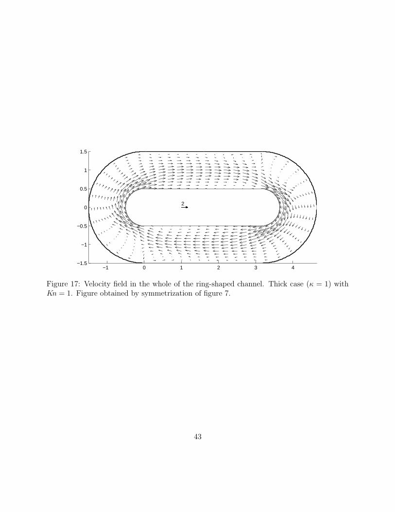
Finally, to give an idea of the circulating flow in the whole ring-shaped device, we plot infigure 17 the velocity field corresponding to the thick channel (κ = 1) with Kn = 1 on which
17

we add the flow in the symmetric part. This is not the result of a computation in the fulldomain but only a plot of the same velocity field with its symmetric image. In this figure,we can more clearly see the two recirculation zones where the circular and straight parts arejoined.
The accuracy of our computations has been studied by using three different grids for eachgeometry: a coarse mesh, a thin mesh, and a very thin mesh. Each mesh has twice as manycells as the coarser mesh in each direction.
For instance for the thick channel with Kn = 1, we used 100 × 24, 200 × 48, and then400×96 cells. First we compared the values obtained for the density profiles averaged in thesection of the channel. We found that the difference between the coarse and the very thinmeshes is less than 1.3 %, while the difference between the thin and the very thin meshes isless than 0.3 %. This means that the coarse mesh is accurate enough to accurately capturethe macroscopic profiles. We also compared the values obtained for the mass flow rate acrossa section. For this quantity, the standard deviation from the average value is a good test ofaccuracy. We found 4 % for the coarse mesh, 1 % for the thin mesh, and then 0.2 % for thevery thin mesh. Consequently, since the mass flow rate is the most important quantity tobe computed in this section, we used the very thin mesh for this case.
The same analysis has been carried out for the other Knudsen numbers, and for themedium and thin channels. The density profiles can be computed with the coarse mesh upto 2 % of accuracy as compared to the very thin mesh. To compute the mass flow rate,the very thin grid must be used, but the standard deviation reaches up to 6 % for themedium channel with Kn = 0.5. Note that for the thin channel, as previously mentioned,the circulating flow effect seems to be so small for Kn = 0.1 that we were not able to correctlycompute the mass flow rate, even with the very thin mesh (1600 × 24 cells).
It is known that the velocity distribution function possesses a discontinuity in the gasaround a convex body [35, 40, 36], and this fact applies to the present problem. That is,the inner curved boundary produces a discontinuity in F in the velocity space. It should bementioned, however, that the present numerical method, which is quite flexible concerningthe geometry, is not designed to describe the discontinuity. For accurate numerical treatmentof the discontinuity produced by a convex body, the reader is referred to for instance [3, 40,42, 39, 43]. But note that for the present numerical tests, an accurate description of thediscontinuity does not seem to be essential: it has been checked on the thick channel that avelocity grid of 80× 80 points instead of 40× 40 gives the same results up to a difference ofless than 0.01%.
5.2.2 Infinite cascade of S-shaped channels
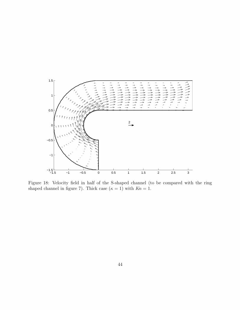
For this test—corresponding to the device presented in figure 4—we also simulate the flowin a single unit by changing the periodic boundary conditions (see section 3.2). We observedthat the results are almost the same as for the ring-shaped channel: the same mass flowrate and the same average macroscopic profiles are obtained. This can be seen in figure 18for the case κ = 1 and Kn = 1 (to be compared with figure 7). The only difference is the
18
direction of the velocity field for x between 0.5 and 3 in the straight part: this direction isthe symmetric (with respect to the horizontal axis) of the direction found for the ring-shapedchannel (look for instance at the location of the recirculation zone). Since there is no othersignificative difference, the other results are not plotted.
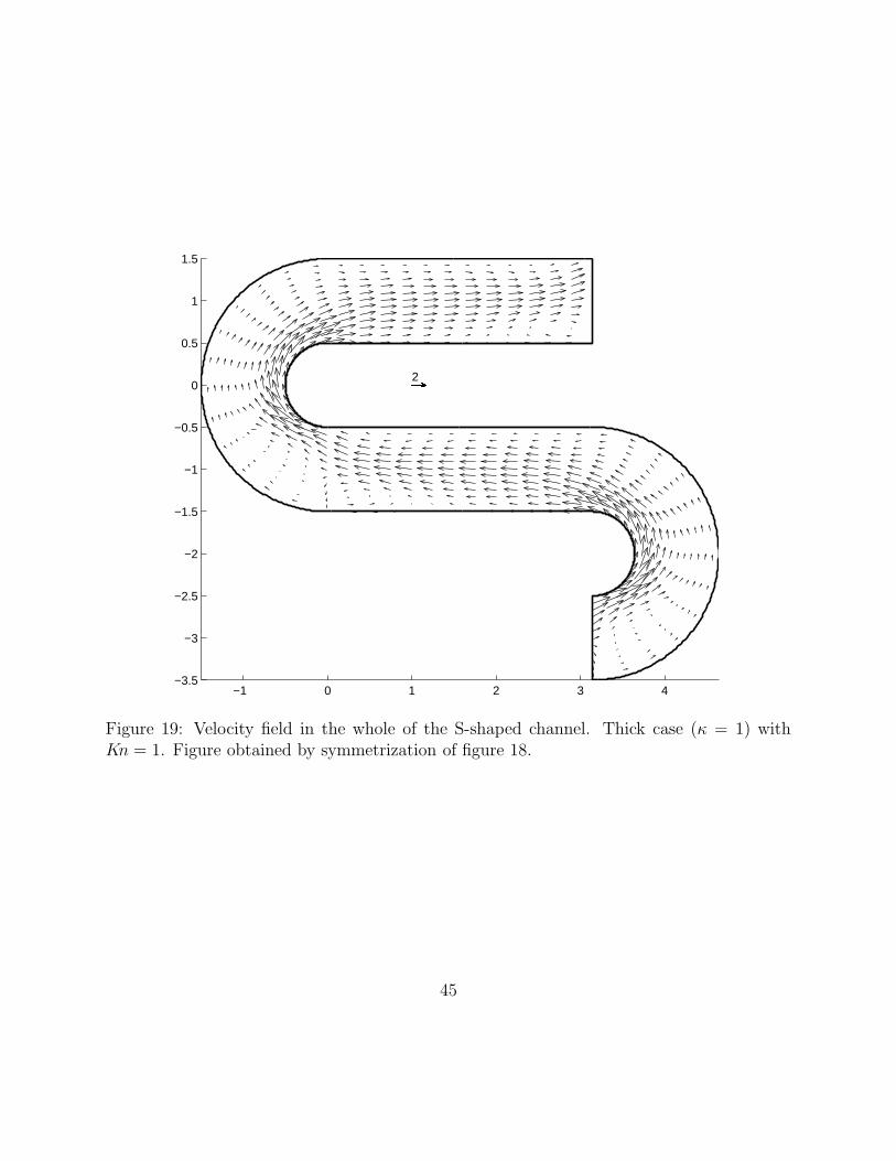
However, we just give in figure 19 a picture of the flow obtained in one period of the fullcascade. As in section 5.2.1, it is obtained by symmetrization of the results obtained in asingle unit.
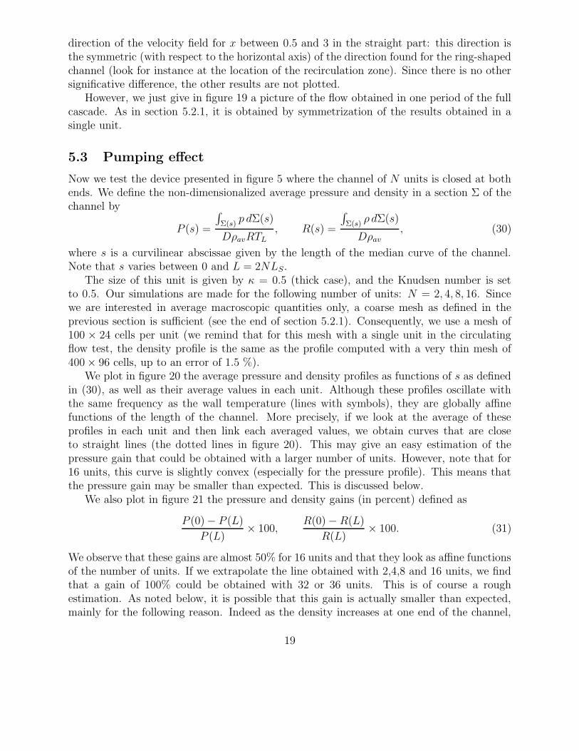
5.3 Pumping effect
Now we test the device presented in figure 5 where the channel of N units is closed at bothends. We define the non-dimensionalized average pressure and density in a section Σ of thechannel by
P (s) =
∫
Σ(s)p dΣ(s)
DρavRTL
, R(s) =
∫
Σ(s)ρ dΣ(s)
Dρav
, (30)
where s is a curvilinear abscissae given by the length of the median curve of the channel.Note that s varies between 0 and L = 2NLS.
The size of this unit is given by κ = 0.5 (thick case), and the Knudsen number is setto 0.5. Our simulations are made for the following number of units: N = 2, 4, 8, 16. Sincewe are interested in average macroscopic quantities only, a coarse mesh as defined in theprevious section is sufficient (see the end of section 5.2.1). Consequently, we use a mesh of100 × 24 cells per unit (we remind that for this mesh with a single unit in the circulatingflow test, the density profile is the same as the profile computed with a very thin mesh of400 × 96 cells, up to an error of 1.5 %).
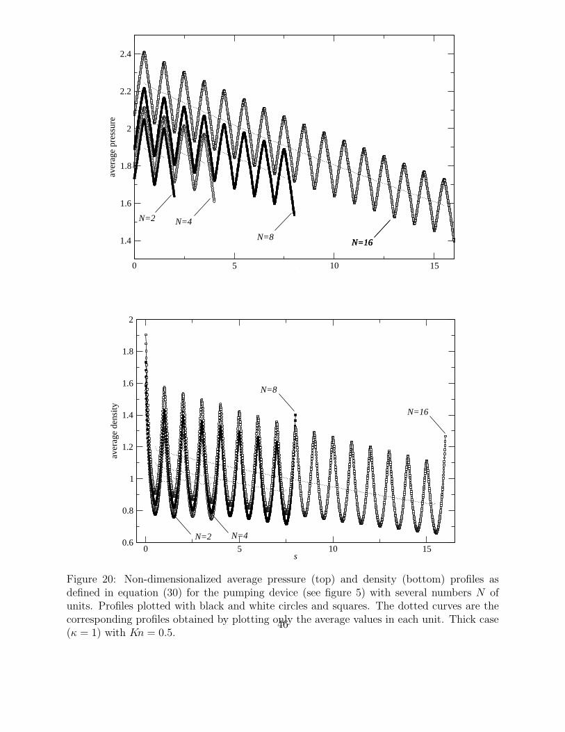
We plot in figure 20 the average pressure and density profiles as functions of s as definedin (30), as well as their average values in each unit. Although these profiles oscillate withthe same frequency as the wall temperature (lines with symbols), they are globally affinefunctions of the length of the channel. More precisely, if we look at the average of theseprofiles in each unit and then link each averaged values, we obtain curves that are closeto straight lines (the dotted lines in figure 20). This may give an easy estimation of thepressure gain that could be obtained with a larger number of units. However, note that for16 units, this curve is slightly convex (especially for the pressure profile). This means thatthe pressure gain may be smaller than expected. This is discussed below.
We also plot in figure 21 the pressure and density gains (in percent) defined as
P (0) − P (L)
P (L)× 100,
R(0) − R(L)
R(L)× 100. (31)
We observe that these gains are almost 50% for 16 units and that they look as affine functionsof the number of units. If we extrapolate the line obtained with 2,4,8 and 16 units, we findthat a gain of 100% could be obtained with 32 or 36 units. This is of course a roughestimation. As noted below, it is possible that this gain is actually smaller than expected,mainly for the following reason. Indeed as the density increases at one end of the channel,
19

the local Knudsen number decreases and the gas becomes more and more dense. Accordingto the kinetic theory, the thermal creep flow should be less and less strong. Consequently, thepumping effect should be weaker and weaker as well. This fact is already visible in figure 20on the pressure profile.
A two dimensional picture of the macroscopic quantities in the 16 unit device can beviewed in figure 22. The periodic temperature field is clearly visible, as well as the increasingof the density and pressure values along the channel. There is almost no variation of thesethree fields along the transverse direction. The velocity field has a more complex structure,but its magnitude is rather small.
5.4 A comparison with the true Boltzmann model
It is generally admitted that the BGK model is physically correct only for flows that areclose to equilibrium. This belief relies on the facts that the structure of the BGK collisionoperator is very simple as compared to the real Boltzmann equation, while it gives the samefluid equations for small Knudsen numbers. However, it is a model for any deviation from alocal equilibrium designed in such a way that it satisfies basic properties of the Boltzmannequation, and for some cases, it turns that the BGK model is able to give precise results thatare quantitatively very close to that of the Boltzmann model, even for intermediate Knudsennumbers. This is in particular true in our study, as it is shown in the following.
We use the test of section 5.3 to compare the BGK and Boltzmann models. The Boltz-mann equation is solved with the classical Direct Simulation Monte-Carlo (DSMC) method(see [8]; the computation was carried out by H. Yoshida basically using the code developedin [1]). The parameters of the DSMC computation are given in [1]. We only mention thatthe grid space used with DSMC has 1.7 times as many cells as in our BGK computations.Note that for DSMC the hard-sphere model is used, hence the definition of the Knudsennumber is not given by (29) but rather by Kn = l0
Dwith l0 = m√
2πd2mρ0
and dm is the diameter
of the molecules (see [41]).We plot the non-dimensional average pressure obtained in pumping devices of 1, 2, 4,
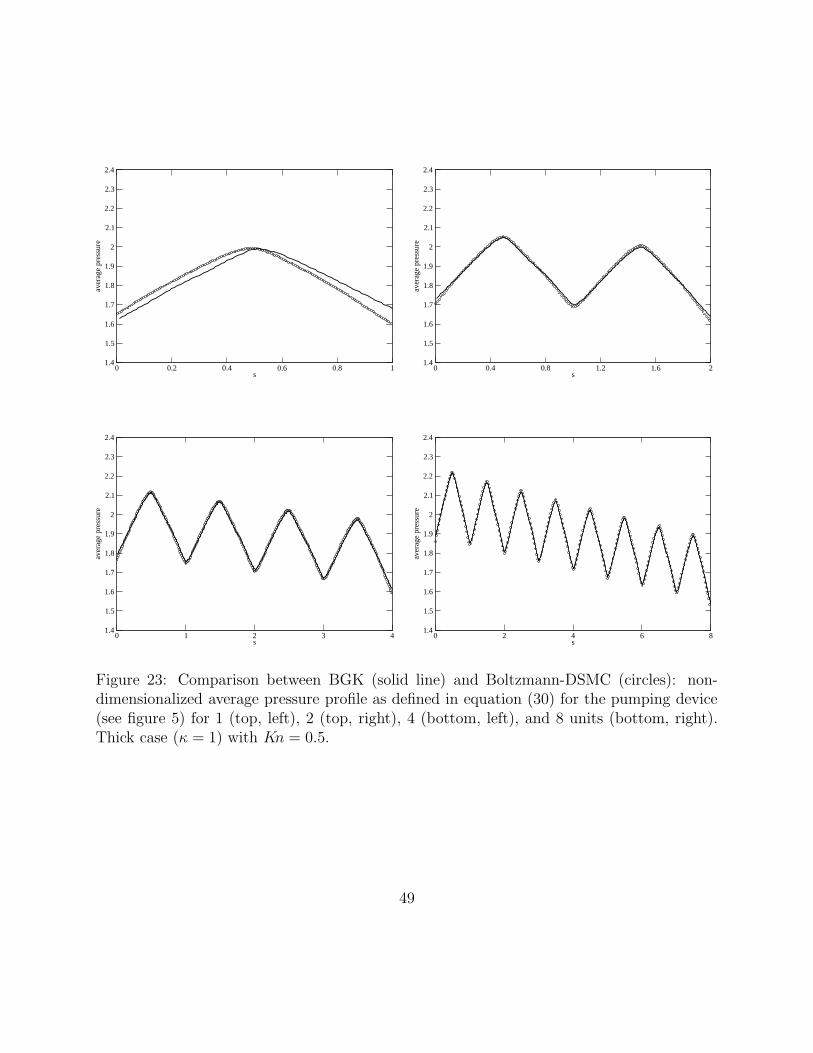
and 8 units with both the BGK and Boltzmann models (figure 23). It appears clearly withthis figure that the two models are very close for 2 to 8 units. More precisely, the maximumrelative difference is found to be lower than 1.7 %. For the 1 unit device, the difference islarger, since the maximum relative difference is 5.2 %.
This clearly demonstrate that the BGK model is accurate enough to describe the flowsconsidered in this study, at least if one is only interested in the average macroscopic quantitiesas the pressure.
Even if the two methods have not been used on the same computer, we give below asignificative comparison on the CPU time consumed for the 8 unit case: the DSMC com-putation required around 15 days with 8 processors Pentium IV (2.4 Ghz) for a global timeof 4 months, while our BGK computation required only 1 day and a half with 6 processorsItanium II (1.5 Ghz) of the SGI Altix 3700, for a global time of 7 days. The main reasonfor the very large CPU time of the DSMC computation is that, due to the long size of the
20

channel, the steady state is reached after a very long physical time.
5.5 Efficiency of the implicit boundary conditions
Here the performance of the implicit treatment of the boundary conditions (see section 4.4)is shown for the pumping device with 8 and 16 units.
For this case, we plot the residual histories at the top of figure 24 for our linearizedimplicit scheme used with explicit and implicit boundary conditions. We observe that thescheme with implicit B.C converges faster: it requires 900 iterations while the scheme withexplicit B.C converges in 1250 iterations. The speed of convergence is thus increased by afactor of 40% for this test case.
For the 16 unit case, the same comparison has not been performed completely, since thecomputation is very long with explicit B.C. However, it seems that the performance of theimplicit B.C is enhanced for this case, as it can be seen at the bottom of figure 24, even ifthe computation with explicit B.C has not been carried at convergence. Indeed, the linearprofile of the residual suggests that the number of iterations to reach the steady state wouldbe around 6500 with the explicit B.C, while with the implicit B.C the algorithm only needs2200 iterations (which is therefore 3 times as fast in this case).
Consequently, the implicit treatment of the B.C seems to speed up the convergence ofour scheme, as well as its scalability. However, the convergence is still globally linear (afterthe rapid decreasing between 0 and 100 iterations), and the scalability is still not very good,since the number of iterations to reach the steady state seems to be a highly increasingfunction of the number of units: for 1, 2, 4, 8, and 16 units, the number of iterations isrespectively 100, 127, 267, 732, and 2272.
It is therefore difficult to compute a flow for a device with more than 32 units with thisalgorithm. We hope that a more sophisticated linear solver could further improve this con-vergence. However, for very long devices, we have proposed an alternative strategy presentedin [2] which consists in using an asymptotic model for the thin channel approximation. Thisallows to compute macroscopic profiles with an arbitrary large number of units very rapidly.
6 Conclusion
In this paper, we have presented a new system of Knudsen pump in a channel that workswithout moving part for a gas under rarefied conditions or in micro-scales. Our device isbased both on the thermal creep effect and on a smoothly varying curvature of the channelthat makes the system very simple.
A new numerical method has been proposed to simulate the pump. This method—whileit is based on a simplified kinetic model—turns out to be very efficient and gives resultsthat are very close to what can be obtained by a classical DSMC, for a comparativelysmall computational time. Our numerical tests demonstrate that a circulating flow can becontrolled in our device, as well as a non negligible pressure ratio in case of a cascade ofseveral units closed at both ends.
21

We hope that this system could be efficiently used on MEMS. Now it should be necessaryto make an intensive optimization study in order to determine the optimal parameters ofour device, so as to maximize the compression ratio. We believe that our numerical methodis an efficient tool for such a study.
We also mention that this new device is the core of a large project in which we alsohave investigated the applicability of simpler macroscopic fluid models derived from kinetictheory by means of asymptotic methods (see [21] for a fluid-dynamic model for small Knudsennumbers and [2] for a simple one dimensional diffusion model). The present study is also arelevant way to validate these fluid models.
However, for a practical application of our device, it should be equally (or even more)important to use a pipe instead of a plane channel. The behavior of the device may beslightly different in this case since, as it has been noted in [4], the pipe resistance to thepressure is larger than that of a plane channel. This results in a device with a weaker flow,but a stronger compression ratio. But for such a system, full three dimensional computationsare necessary, which—for long pipes—requires at present prohibitively large computationaltimes when using kinetic simulations. Therefore, as a preliminary study, it is very useful touse fast kinetic simulations of a 2D plane device.
Acknowledgments
The authors thank Hiroaki Yoshida for the data results of the DSMC computation.
References
[1] K. Aoki, P. Degond, L. Mieussens, M. Nishioka, and S. Takata. Numerical simulation ofa Knudsen pump using the effect of curvature of the channel. In 25st RGD Symposium,Book of Abstracts, St-Petersburg, 2006.
[2] K. Aoki, P. Degond, L. Mieussens, S. Takata, and H. Yoshida. Hydrodynamic modelfor rarefied flows in curved channels. in preparation.
[3] K. Aoki, K. Kanba, and S. Takata. Numerical Analysis of a Supersonic Rarefied GasFlow Past a Flat Plate. Phys. Fluids, 9(4), 1997.
[4] K. Aoki, Y. Sone, S. Takata, K. Takahashi, and G. A. Bird. One-way flow of a rarefiedgas induced in a circular pipe with a periodic temperature distribution. In Timothy J.Bartel and Michael A. Gallis, editors, Rarefied gas dynamics, Vol 1: 22nd InternationalSymposium, volume 585, pages 940–947. AIP, 2001.
[5] V. V. Aristov. Direct methods for solving the Boltzmann equation and study of nonequi-librium flows, volume 60 of Fluid Mechanics and its Applications. Kluwer AcademicPublishers, Dordrecht, 2001.
22

[6] P.L. Bathnagar, E.P. Gross, and M. Krook. A model for collision processes in gases. I.small amplitude processes in charged and neutral one-component systems. Phys. Rev.,94:511–525, 1954.
[7] J. R. Bielenberg and G. H. Brenner. A continuum model of thermal transpiration. J.Fluid Mech., 546:1–23, 2006.
[8] G.A. Bird. Molecular Gas Dynamics and the Direct Simulation of Gas Flows. OxfordScience Publications, 1994.
[9] A. V. Bobylev and S. Rjasanow. Fast deterministic method of solving the Boltzmannequation for hard spheres. Eur. J. Mech. B Fluids, 18(5):869–887, 1999.
[10] C. Buet. A Discrete-Velocity Scheme for the Boltzmann Operator of Rarefied GasDynamics. Transp. Th. Stat. Phys., 25(1):33–60, 1996.
[11] C. Cercignani. The Boltzmann Equation and Its Applications, volume 68. Springer-Verlag, Lectures Series in Mathematics, 1988.
[12] C. Cercignani. Slow rarefied flows: Theory and application to micro-electro-mechanicalsystems, volume 41 of Progress in Mathematical Physics. Birkhauser Verlag, Basel,2006.
[13] B. Dubroca and L. Mieussens. A conservative and entropic discrete-velocity model forrarefied polyatomic gases. In CEMRACS 1999 (Orsay), volume 10 of ESAIM Proc.,pages 127–139 (electronic). Soc. Math. Appl. Indust., Paris, 1999.
[14] F. Filbet, C. Mouhot, and L. Pareschi. Solving the Boltzmann equation in N log2N .SIAM J. Sci. Comput., 28(3):1029–1053 (electronic), 2006.
[15] V. Garzo and A. Santos. Comparison Between the Boltzmann and BGK Equations forUniform Shear Flows. Physica A, 213:426–434, 1995.
[16] A. B. Huang and P. F. Hwang. Test of statistical models for gases with and withoutinternal energy states. Physics of Fluids, 16(4):466–475, 1973.
[17] M. L. Hudson and T. J. Bartel. DSMC simulation of thermal transpiration and acco-modation pump. In R. Brun, R. Campargue, R. Gatignol, and J.-C. Lengrand, editors,Rarefied Gas Dynamics, Vol 1, pages 719–726. CEPADUES, Toulouse, 1999.
[18] G. Karniadakis, A. Beskok, and N. Aluru. Microflows and nanoflows: Fundamentalsand simulation, volume 29 of Interdisciplinary Applied Mathematics. Springer, NewYork, 2005.
[19] M. Knudsen. Eine revision der gleichgewichtsbedingung der gase. Annalen der Physik,336(1):205–229, 1909.
23

[20] M. Knudsen. Thermischer molekulardruck der gase in rohren. Annalen der Physik,338(16):1435–1448, 1910.
[21] C. J. T. Laneryd, K. Aoki, P. Degond, and L. Mieussens. Thermal creep of a slightlyrarefied gas through a channel with curved boundary. In 25st RGD Symposium, Bookof Abstracts, St-Petersburg, 2006.
[22] J. C. Maxwell. On stresses in rarified gases arising from inequalities of temperature.Philosophical Transactions of the Royal Society of London, 170:231–256, 1879.
[23] L. Mieussens. Discrete Velocity Model and Implicit Scheme for the BGK Equation ofRarefied Gas Dynamics. Math. Models and Meth. in Appl. Sci., 8(10):1121–1149, 2000.
[24] L. Mieussens. Discrete-velocity models and numerical schemes for the Boltzmann-BGKequation in plane and axisymmetric geometries. J. Comput. Phys., 162:429–466, 2000.
[25] L. Mieussens. Convergence of a discrete-velocity model for the Boltzmann-BGK equa-tion. Comput. Math. Appl., 41(1-2):83–96, 2001.
[26] T. Ohwada. Structure of normal shock waves: direct numerical analysis of the Boltz-mann equation for hard-sphere molecules. Phys. Fluids A, 5(1):217–234, 1993.
[27] T. Ohwada, Y. Sone, and K. Aoki. Numerical analysis of the shear and thermal creepflows of a rarefied gas over a plane wall on the basis of the linearized boltzmann equationfor hard-sphere molecules. Phys. Fluids A, 1:1588–1599, 1989.
[28] L. Pareschi and G. Russo. Time relaxed Monte Carlo methods for the Boltzmannequation. SIAM J. Sci. Comput., 23(4):1253–1273 (electronic), 2001.
[29] G. Pham-Van-Diep, P. Keeley, E. P. Muntz, and D. P. Weaver. A micromechanicalknudsen compressor. In J. Harvey and G. Lords, editors, Rarefied gas dynamics, vol-ume 1, pages 715–721. Oxford University Press, 1995.
[30] O. Reynolds. Note on thermal transpiration. Proceedings of the Royal Society of London,30:300–302, 1879.
[31] O. Reynolds. On certain dimensional properties of matter in the gaseous state. Part Iand II. Philosophical Transactions of the Royal Society of London, 170:727–845, 1879.
[32] F. Rogier and J. Schneider. A Direct Method For Solving the Boltzmann Equation.Transp. Th. Stat. Phys., 23(1-3):313–338, 1994.
[33] Y. Sone. Thermal creep in rarefied gas. J. Phys. Soc. Jpn, 21:1836–1837, 1966.
[34] Y. Sone. Flows induced by temperature fields in a rarefied gas and their ghost effecton the behavior of a gas in the continuum limit. volume 32 of Annu. Rev. Fluid Mech.,pages 779–811. Annual Reviews, Palo Alto, CA, 2000.
24

[35] Y. Sone. Kinetic theory and fluid dynamics. Modeling and Simulation in Science,Engineering and Technology. Birkhauser Boston Inc., Boston, MA, 2002.
[36] Y. Sone. Molecular gas dynamics: Theory, techniques, and applications. Modeling andSimulation in Science, Engineering and Technology. Birkhauser Boston Inc., Boston,MA, 2007.
[37] Y. Sone, K. Aoki, and H. Sugimoto. The Benard problem for a rarefied gas: formationof steady flow patterns and stability of array of rolls. Phys. Fluids, 9(12):3898–3914,1997.
[38] Y. Sone and K. Sato. Demonstration of a one-way flow of a rarefied gas inducedthrough a pipe without average pressure and temperature gradients. Physics of Fluids,12(7):1864–1868, 2000.
[39] Y. Sone and H. Sugimoto. Kinetic theory analysis of steady evaporating flows froma spherical condensed phase into a vacuum. Physics of Fluids A: Fluid Dynamics,5(6):1491–1511, 1993.
[40] Y. Sone and S. Takata. Discontinuity of the velocity distribution function in a rarefiedgas around a convex body and the slayer at the bottom of the knudsen layer. TransportTheory Statist. Phys., 21(4–6):501–530, 1992.
[41] Y. Sone, Y. Waniguchi, and K. Aoki. One-way flow of a rarefied gas induced in a channelwith a periodic temperature distribution. Physics of Fluids, 8(8):2227–2235, 1996.
[42] H. Sugimoto and Y. Sone. Numerical analysis of steady flows of a gas evaporating fromits cylindrical condensed phase on the basis of kinetic theory. Physics of Fluids A: FluidDynamics, 4(2):419–440, 1992.
[43] S. Takata, Y. Sone, and K. Aoki. Numerical analysis of a uniform flow of a rarefied gaspast a sphere on the basis of the boltzmann equation for hard-sphere molecules. Physicsof Fluids A: Fluid Dynamics, 5(3):716–737, 1993.
[44] S. E. Vargo and E. P. Muntz. Initial results from the first MEMS fabricated thermaltranspiration-driven vacuum pump. In Timothy J. Bartel and Michael A. Gallis, editors,Rarefied gas dynamics, Vol 1: 22nd International Symposium, volume 585, pages 502–509. AIP, 2001.
[45] S. E. Vargo, E. P. Muntz, G. R. Shiflett, and W. C. Tang. Knudsen compressor as amicro- and macroscale vacuum pump without moving parts or fluids. In Papers fromthe 45th National Symposium of the American Vacuum Society, volume 17, pages 2308–2313. AVS, 1999.
[46] P. Welander. On the temperature jump in a rarefied gas. Arkiv fur Fysik, 7(44):507–553,1954.
25

[47] J.Y. Yang and J.C. Huang. Rarefied Flow Computations Using Nonlinear Model Boltz-mann Equations. Journal of Computational Physics, 120:323–339, 1995.
A Jacobian matrices of the Maxwellian mappings ~ρ 7→Mk[~ρ ] and ~ρ 7→ Nk[~ρ ]
Elementary calculus gives the following formulae:
∂~ρMk[~ρ ] = Mk[~ρ ]~m(vk)TA(~ρ )−1
∂~ρNk[~ρ ] = Nk[~ρ ](~m(vk) −1
α4(~ρ )~e )TA(~ρ )−1,
where A(~ρ ) is the following 4 × 4 matrix
A(~ρ ) =∑
k
(
~m(vk)~m(vk)TMk[~ρ ] + ~e
(
~m(vk) −1
α4(~ρ )~e)T
Nk[~ρ ]
)
∆v.
B Diagonal of the relaxation matrix Rn
Using the relations given in appendix A, the first half of this diagonal—related the 2 × 2block structure of Rn—is
∆ni,j,k =
1
τni,j
(
Mk[~ρni,j]~m(vk)
TA(~ρni,j)
−1 ~m(vk)∆v − 1)
,
while the second half is
∆ni,j,k =
1
τni,j
(
Nk[~ρni,j]
(
~m(vk) −1
α4(~ρni,j)~e)T
A(~ρni,j)
−1~e∆v − 1
)
.
26

��������������������������������������������������������������������������������������������������������������������������������������������������������������������������������������������������������������������������������������������������������������������������������������������������������������������������������������������������������������������������������������������
low temperature TLhigh temperature TH
thermal creep flow
of cold moleculesmomentum
momentumof hot molecules
momentum transfered by the molecules to the wall
A
Figure 1: Physical mechanism of the thermal creep flow: the average momentum transferedto the boundary by the molecules coming from the right to point A (large black arrow) islarger than that transfered by molecules coming from the left (small black arrow). Thisresults into a net momentum transfered to the boundary directed from the right to the left(horizontal black arrow). By reaction, the wall makes the gas move from the left to the right(gray arrow).
27
B
D
LS
TH
R
TL
TL
A
Figure 2: Basic unit of our devices : a hook shaped channel.
28
TH TL
TL TH
Figure 3: Ring shaped channel to generate a circulating flow.
29
TH TL
TL
TL
TH
Figure 4: S shaped channel to generate a circulating flow in an infinite cascade.
30
TH TL
TL
TLTH TL
TL
TL
TH
TH
TH
THTL
TL
N units
Figure 5: Closed cascade device to generate a pumping effect.
31

Tk
c
k
k’
f n1
f nk’
f nkmax
N
Rnk,k’
nk∆
n1
gnk’
gnkmax
g
Figure 6: Block (sparse) structure of the matrices of the linearized implicit scheme (22): T(top), Rn with its diagonal sub-blocks ∆n
k (bottom left), and the corresponding unknownvector Un = (fn, gn) (bottom right).
32
−1.5 −1 −0.5 0 0.5 1 1.5 2 2.5 3−1.5
−1
−0.5
0
0.5
1
1.5
2
Figure 7: Velocity field (top) and streamlines (bottom) with magnitude of the velocity ingray scale in half of the ring-shaped channel. The vector field scale is shown with the arrowand the corresponding numeric value printed above it (top). Thick case (κ = 1) with Kn = 1.
33

−2 −1 0 1 2 3 4 5 6−2.5
−2
−1.5
−1
−0.5
0
0.5
1
1.5
2
2.5
1
Figure 8: Velocity field (top) and streamlines (bottom) with magnitude of the velocity ingray scale in half of the ring-shaped channel. Medium case (κ = 0.5) with Kn = 1.
34

−5 0 5 10 15
−5
−4
−3
−2
−1
0
1
2
3
4
5
0.2
Figure 9: Velocity field in half of the ring-shaped channel. Thin case (κ = 0.2) with Kn = 1.
35
−1.5 −1 −0.5 0 0.5 1 1.5 2 2.5 3−1.5
−1
−0.5
0
0.5
1
1.5
2
Figure 10: Velocity field (top) and streamlines (bottom) with magnitude of the velocity ingray scale in half of the ring-shaped channel. Thick case (κ = 1) with Kn = 0.5.
36

−2 −1 0 1 2 3 4 5 6−2.5
−2
−1.5
−1
−0.5
0
0.5
1
1.5
2
2.5
1
Figure 11: Velocity field (top) and streamlines (bottom) with magnitude of the velocity ingray scale in half of the ring-shaped channel. Medium case (κ = 0.5) with Kn = 0.5.
37
−5 0 5 10 15
−5
−4
−3
−2
−1
0
1
2
3
4
5
0.2
Figure 12: Velocity field in half of the ring-shaped channel. Thin case (κ = 0.2) withKn = 0.5.
38

−1.5 −1 −0.5 0 0.5 1 1.5 2 2.5 3−1.5
−1
−0.5
0
0.5
1
1.5
2
Figure 13: Velocity field (top) and streamlines (bottom) with magnitude of the velocity ingray scale in half of the ring-shaped channel. Thick case (κ = 1) with Kn = 0.1.
39
−2 −1 0 1 2 3 4 5 6−2.5
−2
−1.5
−1
−0.5
0
0.5
1
1.5
2
2.5
1
Figure 14: Velocity field (top) and streamlines (bottom) with magnitude of the velocity ingray scale in half of the ring-shaped channel. Medium case (κ = 0.5) with Kn = 0.1.
40

−5 0 5 10 15
−5
−4
−3
−2
−1
0
1
2
3
4
5
0.2
Figure 15: Velocity field in half of the ring-shaped channel. Thin case (κ = 0.2) withKn = 0.1.
41

0 0.1 0.2 0.3 0.4 0.5 0.6 0.7 0.8 0.9 1Knudsen number
0
0.0005
0.001
0.0015
0.002
0.0025
0.003
0.0035
mas
s fl
ow r
ate
κ=1
κ=0.5
κ=0.2
Figure 16: Averaged values of the mass flow rate in the ring-shaped channel as a functionof the Knudsen number. Each curve corresponds to one of the three different channel (thickκ = 1, medium κ = 0.5, and thin κ = 0.2). The horizontal bars represent the standarddeviation of the mass flow rate from its average.
42
−1 0 1 2 3 4−1.5
−1
−0.5
0
0.5
1
1.5
2
Figure 17: Velocity field in the whole of the ring-shaped channel. Thick case (κ = 1) withKn = 1. Figure obtained by symmetrization of figure 7.
43
−1.5 −1 −0.5 0 0.5 1 1.5 2 2.5 3−1.5
−1
−0.5
0
0.5
1
1.5
2
Figure 18: Velocity field in half of the S-shaped channel (to be compared with the ringshaped channel in figure 7). Thick case (κ = 1) with Kn = 1.
44
−1 0 1 2 3 4−3.5
−3
−2.5
−2
−1.5
−1
−0.5
0
0.5
1
1.5
2
Figure 19: Velocity field in the whole of the S-shaped channel. Thick case (κ = 1) withKn = 1. Figure obtained by symmetrization of figure 18.
45
0 5 10 15s
1.4
1.6
1.8
2
2.2
2.4
aver
age
pres
sure
N=2 N=4
N=16N=16N=16N=8
0 5 10 15s
0.6
0.8
1
1.2
1.4
1.6
1.8
2
aver
age
dens
ity
N=4N=2
N=16
N=8
Figure 20: Non-dimensionalized average pressure (top) and density (bottom) profiles asdefined in equation (30) for the pumping device (see figure 5) with several numbers N ofunits. Profiles plotted with black and white circles and squares. The dotted curves are thecorresponding profiles obtained by plotting only the average values in each unit. Thick case(κ = 1) with Kn = 0.5.
46

0 2 4 6 8 10 12 14 16 18N
0
10
20
30
40
50
pres
sure
gai
n (%
)
0 2 4 6 8 10 12 14 16 18N
0
10
20
30
40
50
dens
ity g
ain
(%)
Figure 21: Pressure (top) and density gain (bottom) as defined in equation (31) for thepumping device (see figure 5) with several numbers N of units. Thick case (κ = 1) withKn = 0.5.
47

Temperature [1.1, 2.8]
Density [0.6, 1.9]
Pressure [1.4, 2.5]
Velocity (magnitude) [0, 0.008]
Figure 22: Non-dimensional macroscopic fields in the 16 unit pump. For each field, thebounds used for the linear gray-scale is given. Thick case (κ = 1) with Kn = 0.5.
48
0 0.2 0.4 0.6 0.8 1s
1.4
1.5
1.6
1.7
1.8
1.9
2
2.1
2.2
2.3
2.4
aver
age
pres
sure
0 0.4 0.8 1.2 1.6 2s
1.4
1.5
1.6
1.7
1.8
1.9
2
2.1
2.2
2.3
2.4
aver
age
pres
sure
0 1 2 3 4s
1.4
1.5
1.6
1.7
1.8
1.9
2
2.1
2.2
2.3
2.4
aver
age
pres
sure
0 2 4 6 8s
1.4
1.5
1.6
1.7
1.8
1.9
2
2.1
2.2
2.3
2.4
aver
age
pres
sure
Figure 23: Comparison between BGK (solid line) and Boltzmann-DSMC (circles): non-dimensionalized average pressure profile as defined in equation (30) for the pumping device(see figure 5) for 1 (top, left), 2 (top, right), 4 (bottom, left), and 8 units (bottom, right).Thick case (κ = 1) with Kn = 0.5.
49
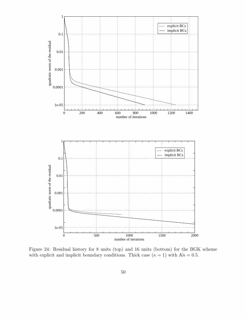
0 200 400 600 800 1000 1200 1400number of iterations
1e-05
0.0001
0.001
0.01
0.1
1
quad
ratic
nor
m o
f th
e re
sidu
al
explicit BCsimplicit BCs
0 500 1000 1500 2000number of iterations
1e-05
0.0001
0.001
0.01
0.1
1
quad
ratic
nor
m o
f th
e re
sidu
al
explicit BCsimplicit BCs
Figure 24: Residual history for 8 units (top) and 16 units (bottom) for the BGK schemewith explicit and implicit boundary conditions. Thick case (κ = 1) with Kn = 0.5.
50