drawing graphs with - graphviz

Drawing graphs with dot

Emden R. Gansner and Eleftherios Koutsofios and Stephen North

January 5, 2015

Abstract

dot draws directed graphs as hierarchies. It runs as a command line pro-gram, web visualization service, or with a compatible graphical interface.Its features include well-tuned layout algorithms for placing nodes and edgesplines, edge labels, “record” shapes with “ports” for drawing data struc-tures; cluster layouts; and an underlying file language for stream-orientedgraph tools. Below is a reduced module dependency graph of an SML-NJcompiler that took 0.23 seconds of user time on a 3 GHz Intel Xeon.

ContMap

FreeMap

Expand

CPSprint

Coder

BaseCoder

ErrorMsg

SparcInstr

GlobalFix

CPS

Hoist

SortedList Intset

CPSopt

Contract

Eta

Closure

Profile

List2

SparcAsCode SparcMCEmit

IEEEReal

SparcCM

CG

SparcMCode

ClosureCallee

Sort

SparcAsEmit

Spill

PrintUtil

CPSsize

Prim

SparcMC

CPScomp

Access

RealConst

SparcAC

Convert

CoreInfo Lambda

CPSgen

Strs

Signs

AbstractFct

ApplyFunctor

Overload

PrintType

Unify

Typecheck

PrintAbsyn

Stream

MLLexFun

Vector

Ascii

LrParserJoinWithArg

Join

MLLrValsFun

CoreLang

NewParse

Index

Misc

TyvarSet

Absyn

Types

Normalize

Modules

ConRep

Instantiate

LrTable Backpatch

PrimTypes PolyCont

Initial

Assembly Math Unsafe

Loader

CInterface CleanUp

CoreFunc

InLine

Fastlib

CoreDummy

Overloads MakeMos

Stamps

IntmapPersStamps

Pathnames

Symbol

Bigint

Dynamic

IntStrMap

ArrayExt

UnionfindSiblings

StrgHash

Env

BasicTypes

Tuples

ModuleUtil

EqTypes

Fixity

TypesUtil

Equal

Variables

BareAbsyn PrintBasics

PrintVal

PrintDec

SigMatch

IntSparcD

IntShare BatchRealDebug BogusDebug

UnixPaths Interact ModuleComp

Importer

IntSparcIntNullD

Linkage

Prof

IntNull

Interp

ProcessFile

FreeLvar LambdaOpt

Translate

OptReorder

CompSparc

MCopt

MCprint

Nonrec MC

InlineOps

Unboxed

1

dot User’s Manual, January 5, 2015 2

1 Basic Graph Drawing

dot draws directed graphs. It reads attributed graph text files and writes drawings,either as graph files or in a graphics format such as GIF, PNG, SVG, PDF, orPostScript.

dot draws graphs in four main phases. Knowing this helps you to understandwhat kind of layouts dot makes and how you can control them. The layout proce-dure used by dot relies on the graph being acyclic. Thus, the first step is to breakany cycles which occur in the input graph by reversing the internal direction ofcertain cyclic edges. The next step assigns nodes to discrete ranks or levels. In atop-to-bottom drawing, ranks determine Y coordinates. Edges that span more thanone rank are broken into chains of “virtual” nodes and unit-length edges. The thirdstep orders nodes within ranks to avoid crossings. The fourth step sets X coordi-nates of nodes to keep edges short, and the final step routes edge splines. This isthe same general approach as most hierarchical graph drawing programs, based onthe work of Warfield [War77], Carpano [Car80] and Sugiyama [STT81]. We referthe reader to [GKNV93] for a thorough explanation of dot’s algorithms.

dot accepts input in the DOT language (cf. Appendix D). This language de-scribes three main kinds of objects: graphs, nodes, and edges. The main (outer-most) graph can be directed (digraph) or undirected graph. Because dot makeslayouts of directed graphs, all the following examples use digraph. (A separatelayout utility, neato, draws undirected graphs [Nor92].) Within a main graph, asubgraph defines a subset of nodes and edges.

Figure 1 is an example graph in the DOT language. Line 1 gives the graphname and type. The lines that follow create nodes, edges, or subgraphs, and setattributes. Names of all these objects may be C identifiers, numbers, or quoted Cstrings. Quotes protect punctuation and white space.

A node is created when its name first appears in the file. An edge is createdwhen nodes are joined by the edge operator ->. In the example, line 2 makesedges from main to parse, and from parse to execute. Running dot on this file (callit graph1.gv)

$ dot -Tps graph1.gv -o graph1.ps

yields the drawing of Figure 2. The command line option -Tps selects PostScript(EPSF) output. graph1.ps may be printed, displayed by a PostScript viewer, orembedded in another document.

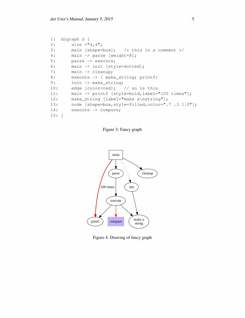
It is often useful to adjust the representation or placement of nodes and edgesin the layout. This is done by setting attributes of nodes, edges, or subgraphs inthe input file. Attributes are name-value pairs of character strings. Figures 3 and 4illustrate some layout attributes. In the listing of Figure 3, line 2 sets the graph’s


1: digraph G {2: main -> parse -> execute;3: main -> init;4: main -> cleanup;5: execute -> make_string;6: execute -> printf7: init -> make_string;8: main -> printf;9: execute -> compare;10: }

Figure 1: Small graph

main

parse

init

cleanup

printf

execute

make_string compare

Figure 2: Drawing of small graph


size to 4,4 (in inches). This attribute controls the size of the drawing; if thedrawing is too large, it is scaled uniformly as necessary to fit.

Node or edge attributes are set off in square brackets. In line 3, the node mainis assigned shape box. The edge in line 4 is straightened by increasing its weight(the default is 1). The edge in line 6 is drawn as a dotted line. Line 8 makes edgesfrom execute to make string and printf. In line 10 the default edge coloris set to red. This affects any edges created after this point in the file. Line 11makes a bold edge labeled 100 times. In line 12, node make_string is givena multi-line label. Line 13 changes the default node to be a box filled with a shadeof blue. The node compare inherits these values.

2 Drawing Attributes

The main attributes that affect graph drawing are summarized in Appendices A, Band C. For more attributes and a more complete description of the attributes, youshould refer to the Graphviz web site, specifically

www.graphviz.org/doc/info/attrs.html

2.1 Node Shapes

Nodes are drawn, by default, with shape=ellipse, width=.75, height=.5and labeled by the node name. Other common shapes include box, circle,record and plaintext. A list of the main node shapes is given in Appendix H.The node shape plaintext is of particularly interest in that it draws a node with-out any outline, an important convention in some kinds of diagrams. In cases wherethe graph structure is of main concern, and especially when the graph is moderatelylarge, the point shape reduces nodes to display minimal content. When drawn, anode’s actual size is the greater of the requested size and the area needed for its textlabel, unless fixedsize=true, in which case the width and height valuesare enforced.

Node shapes fall into two broad categories: polygon-based and record-based.1

All node shapes except record and Mrecord are considered polygonal, andare modeled by the number of sides (ellipses and circles being special cases), anda few other geometric properties. Some of these properties can be specified ina graph. If regular=true, the node is forced to be regular. The parameter

1There is a way to implement custom node shapes, using shape=epsf and the shapefileattribute, and relying on PostScript output. The details are beyond the scope of this user’s guide.Please contact the authors for further information.


1: digraph G {2: size ="4,4";3: main [shape=box]; /* this is a comment */4: main -> parse [weight=8];5: parse -> execute;6: main -> init [style=dotted];7: main -> cleanup;8: execute -> { make_string; printf}9: init -> make_string;10: edge [color=red]; // so is this11: main -> printf [style=bold,label="100 times"];12: make_string [label="make a\nstring"];13: node [shape=box,style=filled,color=".7 .3 1.0"];14: execute -> compare;15: }

Figure 3: Fancy graph

main

parse

init

cleanup

printf

100 times

execute

make astringcompare

Figure 4: Drawing of fancy graph


peripheries sets the number of boundary curves drawn. For example, a dou-blecircle has peripheries=2. The orientation attribute specifies a clock-wise rotation of the polygon, measured in degrees.

The shape polygon exposes all the polygonal parameters, and is useful forcreating many shapes that are not predefined. In addition to the parameters regular,peripheries and orientation, mentioned above, polygons are parameter-ized by number of sides sides, skew and distortion. skew is a floatingpoint number (usually between −1.0 and 1.0) that distorts the shape by slantingit from top-to-bottom, with positive values moving the top of the polygon to theright. Thus, skew can be used to turn a box into a parallelogram. distortionshrinks the polygon from top-to-bottom, with negative values causing the bottomto be larger than the top. distortion turns a box into a trapezoid. A variety ofthese polygonal attributes are illustrated in Figures 6 and 5.

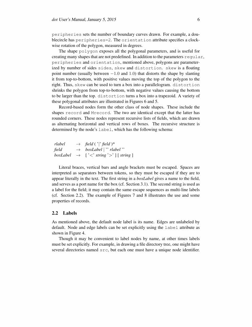
Record-based nodes form the other class of node shapes. These include theshapes record and Mrecord. The two are identical except that the latter hasrounded corners. These nodes represent recursive lists of fields, which are drawnas alternating horizontal and vertical rows of boxes. The recursive structure isdetermined by the node’s label, which has the following schema:

rlabel → field ( ’|’ field )*field → boxLabel | ’’ rlabel ’’boxLabel → [ ’<’ string ’>’ ] [ string ]

Literal braces, vertical bars and angle brackets must be escaped. Spaces areinterpreted as separators between tokens, so they must be escaped if they are toappear literally in the text. The first string in a boxLabel gives a name to the field,and serves as a port name for the box (cf. Section 3.1). The second string is used asa label for the field; it may contain the same escape sequences as multi-line labels(cf. Section 2.2). The example of Figures 7 and 8 illustrates the use and someproperties of records.

2.2 Labels

As mentioned above, the default node label is its name. Edges are unlabeled bydefault. Node and edge labels can be set explicitly using the label attribute asshown in Figure 4.

Though it may be convenient to label nodes by name, at other times labelsmust be set explicitly. For example, in drawing a file directory tree, one might haveseveral directories named src, but each one must have a unique node identifier.


1: digraph G {2: a -> b -> c;3: b -> d;4: a [shape=polygon,sides=5,peripheries=3,color=lightblue,style=filled];5: c [shape=polygon,sides=4,skew=.4,label="hello world"]6: d [shape=invtriangle];7: e [shape=polygon,sides=4,distortion=.7];8: }

Figure 5: Graph with polygonal shapes

a

b

hello world d

e

Figure 6: Drawing of polygonal node shapes

1: digraph structs {2: node [shape=record];3: struct1 [shape=record,label="<f0> left|<f1> mid\ dle|<f2> right"];4: struct2 [shape=record,label="<f0> one|<f1> two"];5: struct3 [shape=record,label="hello\nworld |{ b |{c|<here> d|e}| f}| g | h"];6: struct1 -> struct2;7: struct1 -> struct3;8: }

Figure 7: Records with nested fields


The inode number or full path name are suitable unique identifiers. Then the labelof each node can be set to the file name within its directory.

Multi-line labels can be created by using the escape sequences \n, \l, \r toterminate lines that are centered, or left or right justified.2

Graphs and cluster subgraphs may also have labels. Graph labels appear, bydefault, centered below the graph. Setting labelloc=t centers the label abovethe graph. Cluster labels appear within the enclosing rectangle, in the upper leftcorner. The value labelloc=b moves the label to the bottom of the rectangle.The setting labeljust=r moves the label to the right.

The default font is 14-point Times-Roman, in black. Other font families,sizes and colors may be selected using the attributes fontname, fontsize andfontcolor. Font names should be compatible with the target interpreter. It isbest to use only the standard font families Times, Helvetica, Courier or Symbolas these are guaranteed to work with any target graphics language. For example,Times-Italic, Times-Bold, and Courier are portable; AvanteGarde-DemiOblique isn’t.

For bitmap output, such as GIF or JPG, dot relies on having these fonts avail-able during layout. Most precompiled installations of Graphviz use the fontconfiglibrary for matching font names to available fontfiles. fontconfig comes with aset of utilities for showing matches and installing fonts. Please refer to the font-config documentation, or the external Graphviz FontFAQ or for further details. IfGraphviz is built without fontconfig (which usually means you compiled it fromsource code on your own), the fontpath attribute can specify a list of directo-ries3 which should be searched for the font files. If this is not set, dot will use theDOTFONTPATH environment variable or, if this is not set, the GDFONTPATHenvironment variable. If none of these is set, dot uses a built-in list.

Edge labels are positioned near the center of the edge. Usually, care is taken toprevent the edge label from overlapping edges and nodes. It can still be difficult,in a complex graph, to be certain which edge a label belongs to. If the decorateattribute is set to true, a line is drawn connecting the label to its edge. Sometimesavoiding collisions among edge labels and edges forces the drawing to be biggerthan desired. If labelfloat=true, dot does not try to prevent such overlaps,allowing a more compact drawing.

An edge can also specify additional labels, using headlabel and taillabel,which are be placed near the ends of the edge. The characteristics of these la-bels are specified using the attributes labelfontname, labelfontsize and

2The escape sequence \N is an internal symbol for node names.3For Unix-based systems, this is a concatenated list of pathnames, separated by colons. For

Windows-based systems, the pathnames are separated by semi-colons.


labelfontcolor. These labels are placed near the intersection of the edge andthe node and, as such, may interfere with them. To tune a drawing, the user can setthe labelangle and labeldistance attributes. The former sets the angle,in degrees, which the label is rotated from the angle the edge makes incident withthe node. The latter sets a multiplicative scaling factor to adjust the distance thatthe label is from the node.

2.3 HTML-like Labels

In order to allow a richer collection of attributes at a finer granularity, dot acceptsHTML-like labels using HTML syntax. These are specified using strings that aredelimited by < . . . > rather than double-quotes. Within these delimiters, the stringmust follow the lexical, quoting, and syntactic conventions of HTML.

By using the <TABLE> element, these labels can be viewed as an extensionof and replacement for shape=record. With these, one can alter colors andfonts at the box level, and include images. The PORT attribute of a <TD> elementprovides a port name for the cell (cf. Section 3.1).

Although HTML-like labels are just a special type of label attribute, one fre-quently uses them as though they were a new type of node shape similar to records.Thus, when these are used, one often sees shape=none and margin=0. Alsonote that, as a label, these can be used with edges and graphs as well as nodes.

Figures 9 and 10 give an example of the use of HTML-like labels.

2.4 Graphics Styles

Nodes and edges can specify a color attribute, with black the default. This is thecolor used to draw the node’s shape or the edge. A color value can be a hue-saturation-brightness triple (three floating point numbers between 0 and 1, sepa-rated by commas); one of the colors names listed in Appendix J (borrowed fromsome version of the X window system); or a red-green-blue (RGB) triple4 (threehexadecimal number between 00 and FF, preceded by the character ’#’). Thus, thevalues "orchid", "0.8396,0.4862,0.8549" and "#DA70D6" are threeways to specify the same color. The numerical forms are convenient for scripts ortools that automatically generate colors. Color name lookup is case-insensitive andignores non-alphanumeric characters, so warmgrey and Warm_Grey are equiv-alent.

We can offer a few hints regarding use of color in graph drawings. First, avoidusing too many bright colors. A “rainbow effect” is confusing. It is better to

4A fourth form, RGBA, is also supported, which has the same format as RGB with an additionalfourth hexadecimal number specifying alpha channel or transparency information.


left mid dle right

one two helloworld

b

c d e

f

g h

Figure 8: Drawing of records

1: digraph html {2: abc [shape=none, margin=0, label=<3: <TABLE BORDER="0" CELLBORDER="1" CELLSPACING="0" CELLPADDING="4">4: <TR><TD ROWSPAN="3"><FONT COLOR="red">hello</FONT><BR/>world</TD>5: <TD COLSPAN="3">b</TD>6: <TD ROWSPAN="3" BGCOLOR="lightgrey">g</TD>7: <TD ROWSPAN="3">h</TD>8: </TR>9: <TR><TD>c</TD>

10: <TD PORT="here">d</TD>11: <TD>e</TD>12: </TR>13: <TR><TD COLSPAN="3">f</TD>14: </TR>15: </TABLE>>];16: }

Figure 9: HTML-like labels

helloworld

b

g hc d e

f

Figure 10: Drawing of HTML-like labels


choose a narrower range of colors, or to vary saturation along with hue. Sec-ond, when nodes are filled with dark or very saturated colors, labels seem to bemore readable with fontcolor=white and fontname=Helvetica. (Wealso have PostScript functions for dot that create outline fonts from plain fonts.)Third, in certain output formats, you can define your own color space. For exam-ple, if using PostScript for output, you can redefine nodecolor, edgecolor,or graphcolor in a library file. Thus, to use RGB colors, place the followingline in a file lib.ps.

/nodecolor {setrgbcolor} bind def

Use the -l command line option to load this file.

dot -Tps -l lib.ps file.gv -o file.ps

The style attribute controls miscellaneous graphics features of nodes andedges. This attribute is a comma-separated list of primitives with optional argu-ment lists. The predefined primitives include solid, dashed, dotted, boldand invis. The first four control line drawing in node boundaries and edgesand have the obvious meaning. The value invis causes the node or edge to beleft undrawn. The style for nodes can also include filled, diagonals androunded. filled shades inside the node using the color fillcolor. If thisis not set, the value of color is used. If this also is unset, light grey5 is used as thedefault. The diagonals style causes short diagonal lines to be drawn betweenpairs of sides near a vertex. The rounded style rounds polygonal corners.

User-defined style primitives can be implemented as custom PostScript proce-dures. Such primitives are executed inside the gsave context of a graph, node,or edge, before any of its marks are drawn. The argument lists are translated toPostScript notation. For example, a node with style="setlinewidth(8)"is drawn with a thick outline. Here, setlinewidth is a PostScript built-in, butuser-defined PostScript procedures are called the same way. The definition of theseprocedures can be given in a library file loaded using -l as shown above.

Edges have a dir attribute to set arrowheads. dir may be forward (thedefault), back, both, or none. This refers only to where arrowheads are drawn,and does not change the underlying graph. For example, setting dir=back causesan arrowhead to be drawn at the tail and no arrowhead at the head, but it does notexchange the endpoints of the edge. The attributes arrowhead and arrowtailspecify the style of arrowhead, if any, which is used at the head and tail ends ofthe edge. Allowed values are normal, inv, dot, invdot, odot, invodot

5The default is black if the output format is MIF, or if the shape is point.


and none (cf. Appendix I). The attribute arrowsize specifies a multiplica-tive factor affecting the size of any arrowhead drawn on the edge. For example,arrowsize=2.0 makes the arrow twice as long and twice as wide.

In terms of style and color, clusters act somewhat like large box-shaped nodes,in that the cluster boundary is drawn using the cluster’s color attribute and, ingeneral, the appearance of the cluster is affected the style, color and fillcolorattributes.

If the root graph has a bgcolor attribute specified, this color is used as thebackground for the entire drawing, and also serves as the default fill color.

2.5 Drawing Orientation, Size and Spacing

Two attributes that play an important role in determining the size of a dot drawingare nodesep and ranksep. The first specifies the minimum distance, in inches,between two adjacent nodes on the same rank. The second deals with rank sepa-ration, which is the minimum vertical space between the bottoms of nodes in onerank and the tops of nodes in the next. The ranksep attribute sets the rank separa-tion, in inches. Alternatively, one can have ranksep=equally. This guaranteesthat all of the ranks are equally spaced, as measured from the centers of nodes onadjacent ranks. In this case, the rank separation between two ranks is at least thedefault rank separation. As the two uses of ranksep are independent, both canbe set at the same time. For example, ranksep="1.0 equally" causes ranksto be equally spaced, with a minimum rank separation of 1 inch.

Often a drawing made with the default node sizes and separations is too bigfor the target printer or for the space allowed for a figure in a document. Thereare several ways to try to deal with this problem. First, we will review how dotcomputes the final layout size.

A layout is initially made internally at its “natural” size, using default settings(unless ratio=compress was set, as described below). There is no bound onthe size or aspect ratio of the drawing, so if the graph is large, the layout is alsolarge. If you don’t specify size or ratio, then the natural size layout is printed.

The easiest way to control the output size of the drawing is to set size="x,y"in the graph file (or on the command line using -G). This determines the size of thefinal layout. For example, size="7.5,10" fits on an 8.5x11 page (assumingthe default page orientation) no matter how big the initial layout.

ratio also affects layout size. There are a number of cases, depending on thesettings of size and ratio.

Case 1. ratio was not set. If the drawing already fits within the given size,then nothing happens. Otherwise, the drawing is reduced uniformly enough tomake the critical dimension fit.


If ratio was set, there are four subcases.Case 2a. If ratio=x where x is a floating point number, then the drawing

is scaled up in one dimension to achieve the requested ratio expressed as drawingheight/width. For example, ratio=2.0 makes the drawing twice as high as itis wide. Then the layout is scaled using size as in Case 1.

Case 2b. If ratio=fill and size=x, y was set, then the drawing is scaledup in one dimension to achieve the ratio y/x. Then scaling is performed as in Case1. The effect is that all of the bounding box given by size is filled.

Case 2c. If ratio=compress and size=x, y was set, then the initial layoutis compressed to attempt to fit it in the given bounding box. This trades off lay-out quality, balance and symmetry in order to pack the layout more tightly. Thenscaling is performed as in Case 1.

Case 2d. If ratio=auto and the page attribute is set and the graph cannotbe drawn on a single page, then size is ignored and dot computes an “ideal” size.In particular, the size in a given dimension will be the smallest integral multipleof the page size in that dimension which is at least half the current size. The twodimensions are then scaled independently to the new size.

If rotate=90 is set, or orientation=landscape, then the drawing isrotated 90◦ into landscape mode. The X axis of the layout would be along the Yaxis of each page. This does not affect dot’s interpretation of size, ratio orpage.

At this point, if page is not set, then the final layout is produced as one page.If page=x, y is set, then the layout is printed as a sequence of pages which

can be tiled or assembled into a mosaic. Common settings are page="8.5,11"or page="11,17". These values refer to the full size of the physical device; theactual area used will be reduced by the margin settings. (For printer output, thedefault is 0.5 inches; for bitmap-output, the X and Y margins are 10 and 2 points,respectively.) For tiled layouts, it may be helpful to set smaller margins. This canbe done by using the margin attribute. This can take a single number, used to setboth margins, or two numbers separated by a comma to set the x and y marginsseparately. As usual, units are in inches. Although one can set margin=0, un-fortunately, many bitmap printers have an internal hardware margin that cannot beoverridden.

The order in which pages are printed can be controlled by the pagedir at-tribute. Output is always done using a row-based or column-based ordering, andpagedir is set to a two-letter code specifying the major and minor directions. Forexample, the default is BL, specifying a bottom-to-top (B) major order and a left-to-right (L) minor order. Thus, the bottom row of pages is emitted first, from leftto right, then the second row up, from left to right, and finishing with the top row,from left to right. The top-to-bottom order is represented by T and the right-to-left


order by R.If center=true and the graph can be output on one page, using the default

page size of 8.5 by 11 inches if page is not set, the graph is repositioned to becentered on that page.

A common problem is that a large graph drawn at a small size yields unreadablenode labels. To make larger labels, something has to give. There is a limit to theamount of readable text that can fit on one page. Often you can draw a smallergraph by extracting an interesting piece of the original graph before running dot.We have some tools that help with this.

sccmap decompose the graph into strongly connected components

tred compute transitive reduction (remove edges implied by transitivity)

gvpr graph processor to select nodes or edges, and contract or remove the rest ofthe graph

unflatten improve aspect ratio of trees by staggering the lengths of leaf edges

With this in mind, here are some thing to try on a given graph:

1. Increase the node fontsize.

2. Use smaller ranksep and nodesep.

3. Use ratio=auto.

4. Use ratio=compress and give a reasonable size.

5. A sans serif font (such as Helvetica) may be more readable than Times whenreduced.

2.6 Node and Edge Placement

Attributes in dot provide many ways to adjust the large-scale layout of nodes andedges, as well as fine-tune the drawing to meet the user’s needs and tastes. Thissection discusses these attributes6.

Sometimes it is natural to make edges point from left to right instead of fromtop to bottom. If rankdir=LR in the top-level graph, the drawing is rotated in thisway. TB (top to bottom) is the default. The mode rankdir=BT is useful for draw-ing upward-directed graphs. For completeness, one can also have rankdir=RL.

6For completeness, we note that dot also provides access to various parameters which play techni-cal roles in the layout algorithms. These include mclimit, nslimit, nslimit1, remincrossand searchsize.


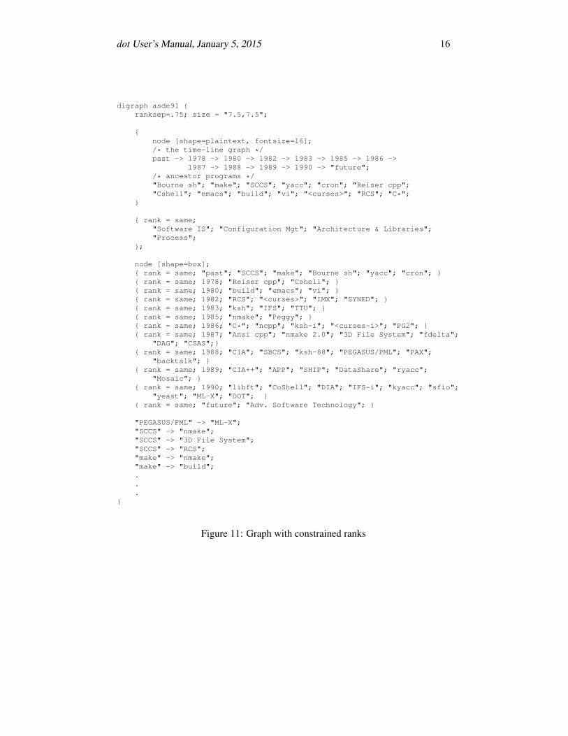
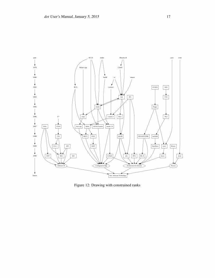
In graphs with time-lines, or in drawings that emphasize source and sink nodes,you may need to constrain rank assignments. The rank of a subgraph may be setto same, min, source, max or sink. A value same causes all the nodes in thesubgraph to occur on the same rank. If set to min, all the nodes in the subgraphare guaranteed to be on a rank at least as small as any other node in the layout7.This can be made strict by setting rank=source, which forces the nodes in thesubgraph to be on some rank strictly smaller than the rank of any other nodes(except those also specified by min or source subgraphs). The values max orsink play an analogous role for the maximum rank. Note that these constraintsinduce equivalence classes of nodes. If one subgraph forces nodes A and B to beon the same rank, and another subgraph forces nodes C and B to share a rank, thenall nodes in both subgraphs must be drawn on the same rank. Figures 11 and 12illustrate using subgraphs for controlling rank assignment.

In some graphs, the left-to-right ordering of nodes is important. If a subgraphhas ordering=out, then out-edges within the subgraph that have the same tailnode wll fan-out from left to right in their order of creation. (Also note that flatedges involving the head nodes can potentially interfere with their ordering.)

There are many ways to fine-tune the layout of nodes and edges. For example,if the nodes of an edge both have the same group attribute, dot tries to keepthe edge straight and avoid having other edges cross it. The weight of an edgeprovides another way to keep edges straight. An edge’s weight suggests somemeasure of an edge’s importance; thus, the heavier the weight, the closer togetherits nodes should be. dot causes edges with heavier weights to be drawn shorter andstraighter.

Edge weights also play a role when nodes are constrained to the same rank.Edges with non-zero weight between these nodes are aimed across the rank inthe same direction (left-to-right, or top-to-bottom in a rotated drawing) as far aspossible. This fact may be exploited to adjust node ordering by placing invisibleedges (style="invis") where needed.

The end points of edges adjacent to the same node can be constrained using thesamehead and sametail attributes. Specifically, all edges with the same headand the same value of samehead are constrained to intersect the head node at thesame point. The analogous property holds for tail nodes and sametail.

During rank assignment, the head node of an edge is constrained to be on ahigher rank than the tail node. If the edge has constraint=false, however,this requirement is not enforced.

In certain circumstances, the user may desire that the end points of an edgenever get too close. This can be obtained by setting the edge’s minlen attribute.

7Recall that the minimum rank occurs at the top of a drawing.


digraph asde91 {ranksep=.75; size = "7.5,7.5";

{node [shape=plaintext, fontsize=16];/* the time-line graph */past -> 1978 -> 1980 -> 1982 -> 1983 -> 1985 -> 1986 ->

1987 -> 1988 -> 1989 -> 1990 -> "future";/* ancestor programs */"Bourne sh"; "make"; "SCCS"; "yacc"; "cron"; "Reiser cpp";"Cshell"; "emacs"; "build"; "vi"; "<curses>"; "RCS"; "C*";

}

{ rank = same;"Software IS"; "Configuration Mgt"; "Architecture & Libraries";"Process";

};

node [shape=box];{ rank = same; "past"; "SCCS"; "make"; "Bourne sh"; "yacc"; "cron"; }{ rank = same; 1978; "Reiser cpp"; "Cshell"; }{ rank = same; 1980; "build"; "emacs"; "vi"; }{ rank = same; 1982; "RCS"; "<curses>"; "IMX"; "SYNED"; }{ rank = same; 1983; "ksh"; "IFS"; "TTU"; }{ rank = same; 1985; "nmake"; "Peggy"; }{ rank = same; 1986; "C*"; "ncpp"; "ksh-i"; "<curses-i>"; "PG2"; }{ rank = same; 1987; "Ansi cpp"; "nmake 2.0"; "3D File System"; "fdelta";

"DAG"; "CSAS";}{ rank = same; 1988; "CIA"; "SBCS"; "ksh-88"; "PEGASUS/PML"; "PAX";

"backtalk"; }{ rank = same; 1989; "CIA++"; "APP"; "SHIP"; "DataShare"; "ryacc";

"Mosaic"; }{ rank = same; 1990; "libft"; "CoShell"; "DIA"; "IFS-i"; "kyacc"; "sfio";

"yeast"; "ML-X"; "DOT"; }{ rank = same; "future"; "Adv. Software Technology"; }

"PEGASUS/PML" -> "ML-X";"SCCS" -> "nmake";"SCCS" -> "3D File System";"SCCS" -> "RCS";"make" -> "nmake";"make" -> "build";...

}

Figure 11: Graph with constrained ranks


past

1978

1980

1982

1983

1985

1986

1987

1988

1989

1990

future

Bourne sh

Cshell

ksh

make

build

nmake

SCCS

RCS

3D File System

yacc

ryacc

cron

yeast

Reiser cpp

ncpp

emacs

nmake 2.0

vi

<curses>

<curses-i>

fdelta

SBCS

C*

CSAS

Software IS

Adv. Software Technology

Configuration Mgt Architecture & Libraries Process

IMX

TTU

SYNED

Peggy

ksh-i

ksh-88

IFS

IFS-isfio

PG2

PEGASUS/PML

Ansi cpp

backtalk

CoShell

PAX

DAG

DIADOT

CIA

CIA++

ML-X

SHIP DataShareAPP

kyacc

Mosaic

libft

Figure 12: Drawing with constrained ranks


This defines the minimum difference between the ranks of the head and tail. Forexample, if minlen=2, there will always be at least one intervening rank betweenthe head and tail. Note that this is not concerned with the geometric distance be-tween the two nodes.

Fine-tuning should be approached cautiously. dot works best when it canmakes a layout without much “help” or interference in its placement of individualnodes and edges. Layouts can be adjusted somewhat by increasing the weight ofcertain edges, or by creating invisible edges or nodes using style=invis, andsometimes even by rearranging the order of nodes and edges in the file. But this canbackfire because the layouts are not necessarily stable with respect to changes inthe input graph. One last adjustment can invalidate all previous changes and makea very bad drawing. A future project we have in mind is to combine the mathemat-ical layout techniques of dot with an interactive front-end that allows user-definedhints and constraints.

3 Advanced Features

3.1 Node Ports

A node port is a point where edges can attach to a node. (When an edge is notattached to a port, it is aimed at the node’s center and the edge is clipped at thenode’s boundary.)

There are two types of ports. Ports based on the 8 compass points "n", "ne","e", "se", "s", "sw", "w" or "nw" can be specified for any node. The endof the edge will then be aimed at that position on the node. Thus, if se port isspecified, the edge will connect to the node at its southeast “corner”.

In addition, nodes with a record shape can use the record structure to defineports, while HTML-like labels with tables can make any cell a port using the PORTattribute of a <TD> element. If a record box or table cell defines a port name, anedge can use that port name to indicate that it should be aimed at the center of thebox. (By default, the edge is clipped to the box’s boundary.)

There are also two ways to specify ports. One way is to use an edge’s headportand tailport attributes, e.g.

a -> b [tailport=se]

Alternatively, the portname can be used to modify the node name as part of theedge declaration using the syntax node name:port name. Thus, another way tohandle the example given above would be

a -> b:se


Since a record box has its own corners, one can add a compass point port torecord name port. Thus, the edge

a -> b:f0:se

will attach to the southeast corner of the box in record node b whose port name isf0.

Figure 13 illustrates the declaration and use of port names in record nodes, withthe resulting drawing shown in Figure 14.

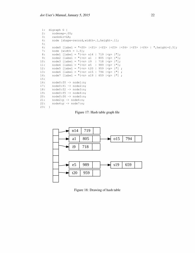
Figures 15 and 16 give another example of the use of record nodes and ports.This repeats the example of Figures 7 and 8 but now using ports as connectorsfor edges. Note that records sometimes look better if their input height is set to asmall value, so the text labels dominate the actual size, as illustrated in Figure 13.Otherwise the default node size (.75 by .5) is assumed, as in Figure 16. Theexample of Figures 17 and 18 uses left-to-right drawing in a layout of a hash table.

3.2 Clusters

A cluster is a subgraph placed in its own distinct rectangle of the layout. A sub-graph is recognized as a cluster when its name has the prefix cluster. (If thetop-level graph has clusterrank=none, this special processing is turned off).Labels, font characteristics and the labelloc attribute can be set as they wouldbe for the top-level graph, though cluster labels appear above the graph by default.For clusters, the label is left-justified by default; if labeljust="r", the label isright-justified. The color attribute specifies the color of the enclosing rectangle.In addition, clusters may have style="filled", in which case the rectangleis filled with the color specified by fillcolor before the cluster is drawn. (Iffillcolor is not specified, the cluster’s color attribute is used.)

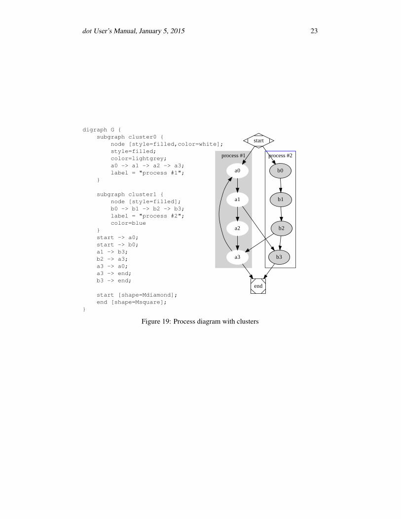
Clusters are drawn by a recursive technique that computes a rank assignmentand internal ordering of nodes within clusters. Figure 19 through 21 are clusterlayouts and the corresponding graph files.


1: digraph g {2: node [shape = record,height=.1];3: node0[label = "<f0> |<f1> G|<f2> "];4: node1[label = "<f0> |<f1> E|<f2> "];5: node2[label = "<f0> |<f1> B|<f2> "];6: node3[label = "<f0> |<f1> F|<f2> "];7: node4[label = "<f0> |<f1> R|<f2> "];8: node5[label = "<f0> |<f1> H|<f2> "];9: node6[label = "<f0> |<f1> Y|<f2> "];

10: node7[label = "<f0> |<f1> A|<f2> "];11: node8[label = "<f0> |<f1> C|<f2> "];12: "node0":f2 -> "node4":f1;13: "node0":f0 -> "node1":f1;14: "node1":f0 -> "node2":f1;15: "node1":f2 -> "node3":f1;16: "node2":f2 -> "node8":f1;17: "node2":f0 -> "node7":f1;18: "node4":f2 -> "node6":f1;19: "node4":f0 -> "node5":f1;20: }

Figure 13: Binary search tree using records

G

E R

B F

A C

H Y

Figure 14: Drawing of binary search tree


1: digraph structs {2: node [shape=record];3: struct1 [shape=record,label="<f0> left|<f1> middle|<f2> right"];4: struct2 [shape=record,label="<f0> one|<f1> two"];5: struct3 [shape=record,label="hello\nworld |{ b |{c|<here> d|e}| f}| g | h"];6: struct1:f1 -> struct2:f0;7: struct1:f2 -> struct3:here;8: }

Figure 15: Records with nested fields (revisited)

left middle right

one two helloworld

b

c d e

f

g h

Figure 16: Drawing of records (revisited)


1: digraph G {2: nodesep=.05;3: rankdir=LR;4: node [shape=record,width=.1,height=.1];5:6: node0 [label = "<f0> |<f1> |<f2> |<f3> |<f4> |<f5> |<f6> | ",height=2.5];7: node [width = 1.5];8: node1 [label = "{<n> n14 | 719 |<p> }"];9: node2 [label = "{<n> a1 | 805 |<p> }"];

10: node3 [label = "{<n> i9 | 718 |<p> }"];11: node4 [label = "{<n> e5 | 989 |<p> }"];12: node5 [label = "{<n> t20 | 959 |<p> }"] ;13: node6 [label = "{<n> o15 | 794 |<p> }"] ;14: node7 [label = "{<n> s19 | 659 |<p> }"] ;15:16: node0:f0 -> node1:n;17: node0:f1 -> node2:n;18: node0:f2 -> node3:n;19: node0:f5 -> node4:n;20: node0:f6 -> node5:n;21: node2:p -> node6:n;22: node4:p -> node7:n;23: }

Figure 17: Hash table graph file

n14 719

a1 805

i9 718

e5 989

t20 959

o15 794

s19 659

Figure 18: Drawing of hash table


digraph G {subgraph cluster0 {

node [style=filled,color=white];style=filled;color=lightgrey;a0 -> a1 -> a2 -> a3;label = "process #1";

}

subgraph cluster1 {node [style=filled];b0 -> b1 -> b2 -> b3;label = "process #2";color=blue

}start -> a0;start -> b0;a1 -> b3;b2 -> a3;a3 -> a0;a3 -> end;b3 -> end;

start [shape=Mdiamond];end [shape=Msquare];

}

process #1 process #2

a0

a1

a2

b3a3

end

b0

b1

b2

start

Figure 19: Process diagram with clusters


If the top-level graph has the compound attribute set to true, dot will allowedges connecting nodes and clusters. This is accomplished by an edge definingan lhead or ltail attribute. The value of these attributes must be the name ofa cluster containing the head or tail node, respectively. In this case, the edge isclipped at the cluster boundary. All other edge attributes, such as arrowheador dir, are applied to the truncated edge. For example, Figure 22 shows a graphusing the compound attribute and the resulting diagram.

3.3 Concentrators

Setting concentrate=true on the top-level graph enables an edge mergingtechnique to reduce clutter in dense layouts. Edges are merged when they runparallel, have a common endpoint and have length greater than 1. A beneficialside-effect in fixed-sized layouts is that removal of these edges often permits larger,more readable labels. While concentrators in dot look somewhat like Newbery’s[New89], they are found by searching the edges in the layout, not by detectingcomplete bipartite graphs in the underlying graph. Thus the dot approach runsmuch faster but doesn’t collapse as many edges as Newbery’s algorithm.

4 Command Line Options

By default, dot operates in filter mode, reading a graph from stdin, and writingthe graph on stdout in the DOT format with layout attributes appended. dotsupports a variety of command-line options:

-Tformat sets the format of the output. Allowed values for format are:

bmp Windows bitmap format.

canon Prettyprint input; no layout is done.

dot Attributed DOT. Prints input with layout information attached as attributes,cf. Appendix F.

fig FIG output.

gd GD format. This is the internal format used by the GD Graphics Library. Analternate format is gd2.

gif GIF output.

imap Produces map files for server-side image maps. This can be combined witha graphical form of the output, e.g., using -Tgif or -Tjpg, in web pagesto attach links to nodes and edges.


1:digraph G {2: size="8,6"; ratio=fill; node[fontsize=24];3:4: ciafan->computefan; fan->increment; computefan->fan; stringdup->fatal;5: main->exit; main->interp_err; main->ciafan; main->fatal; main->malloc;6: main->strcpy; main->getopt; main->init_index; main->strlen; fan->fatal;7: fan->ref; fan->interp_err; ciafan->def; fan->free; computefan->stdprintf;8: computefan->get_sym_fields; fan->exit; fan->malloc; increment->strcmp;9: computefan->malloc; fan->stdsprintf; fan->strlen; computefan->strcmp;10: computefan->realloc; computefan->strlen; debug->sfprintf; debug->strcat;11: stringdup->malloc; fatal->sfprintf; stringdup->strcpy; stringdup->strlen;12: fatal->exit;13:14: subgraph "cluster_error.h" { label="error.h"; interp_err; }15:16: subgraph "cluster_sfio.h" { label="sfio.h"; sfprintf; }17:18: subgraph "cluster_ciafan.c" { label="ciafan.c"; ciafan; computefan;19: increment; }20:21: subgraph "cluster_util.c" { label="util.c"; stringdup; fatal; debug; }22:23: subgraph "cluster_query.h" { label="query.h"; ref; def; }24:25: subgraph "cluster_field.h" { get_sym_fields; }26:27: subgraph "cluster_stdio.h" { label="stdio.h"; stdprintf; stdsprintf; }28:29: subgraph "cluster_<libc.a>" { getopt; }30:31: subgraph "cluster_stdlib.h" { label="stdlib.h"; exit; malloc; free; realloc; }32:33: subgraph "cluster_main.c" { main; }34:35: subgraph "cluster_index.h" { init_index; }36:37: subgraph "cluster_string.h" { label="string.h"; strcpy; strlen; strcmp; strcat; }38:}

Figure 20: Call graph file


error.h

sfio.h

ciafan.cutil.c

query.h

stdio.h stdlib.hstring.h

ciafan

computefan def

fan

mallocstrlen stdprintfget_sym_fieldsstrcmp realloc

increment

fatal

exit

interp_errref

freestdsprintf

stringdup

strcpy sfprintf

main

getopt init_indexdebug

strcat

Figure 21: Call graph with labeled clusters


digraph G {compound=true;subgraph cluster0 {

a -> b;a -> c;b -> d;c -> d;

}subgraph cluster1 {

e -> g;e -> f;

}b -> f [lhead=cluster1];d -> e;c -> g [ltail=cluster0,

lhead=cluster1];c -> e [ltail=cluster0];d -> h;

}

a

b c

d

f

e

g

h

Figure 22: Graph with edges on clusters


cmapx Produces HTML map files for client-side image maps.

pdf Adobe PDF via the Cairo library. We have seen problems when embeddinginto other documents. Instead, use -Tps2 as described below.

plain Simple, line-based ASCII format. Appendix E describes this output. Analternate format is plain-ext, which provides port names on the head andtail nodes of edges.

png PNG (Portable Network Graphics) output.

ps PostScript (EPSF) output.

ps2 PostScript (EPSF) output with PDF annotations. This output should be dis-tilled into PDF, such as for pdflatex, before being included in a document.(Use ps2pdf; epstopdf doesn’t handle %%BoundingBox: (atend).)

svg SVG output. The alternate form svgz produces compressed SVG.

vrml VRML output.

wbmp Wireless BitMap (WBMP) format.

-Gname=value sets a graph attribute default value. Often it is convenient to setsize, pagination, and related values on the command line rather than in the graphfile. The analogous flags -N or -E set default node or edge attributes. Note thatfile contents override command line arguments.

-llibfile specifies a device-dependent graphics library file. Multiple librariesmay be given. These names are passed to the code generator at the beginning ofoutput.

-ooutfile writes output into file outfile.-v requests verbose output. In processing large layouts, the verbose messages

may give some estimate of dot’s progress.-V prints the version number and exits.

5 Miscellaneous

In the top-level graph heading, a graph may be declared a strict digraphor a strict graph. This forbids the creation of multi-edges, i.e., there can beat most one edge with a given tail node and head node in the directed case. Forundirected graphs, there can be at most one edge connected to the same two nodes.Subsequent edge statements using the same two nodes will identify the edge withthe previously defined one and apply any attributes given in the edge statement.


Nodes, edges and graphs may have a URL attribute. In certain output formats(ps2, imap, cmapx, or svg), this information is integrated in the output so thatnodes, edges and clusters become active links when displayed with the appropriatetools. Typically, URLs attached to top-level graphs serve as base URLs, supportingrelative URLs on components. When the output format is imap, or cmapx, asimilar processing takes place with the headURL and tailURL attributes.

For certain formats (ps, fig or svg), comment attributes can be used toembed human-readable notations in the output.

6 Conclusions

dot produces pleasing hierarchical drawings and can be applied in many settings.Since the basic algorithms of dot work well, we have a good basis for fur-

ther research into problems such as methods for drawing large graphs and on-line(animated) graph drawing.

7 Acknowledgments

We thank Phong Vo for his advice about graph drawing algorithms and program-ming. The graph library uses Phong’s splay tree dictionary library. Also, the usersof dag, the predecessor of dot, gave us many good suggestions. Guy Jacobson andRandy Hackbarth reviewed earlier drafts of this manual, and Emden contributedsubstantially to the current revision. John Ellson wrote the generalized polygonshape and spent considerable effort to make it robust and efficient. He also wrotethe GIF and ISMAP generators and other tools to bring Graphviz to the web.


References

[Car80] M. Carpano. Automatic display of hierarchized graphs for computeraided decision analysis. IEEE Transactions on Software Engineering,SE-12(4):538–546, April 1980.

[GKNV93] Emden R. Gansner, Eleftherios Koutsofios, Stephen C. North, andKiem-Phong Vo. A Technique for Drawing Directed Graphs. IEEETrans. Sofware Eng., 19(3):214–230, May 1993.

[New89] Frances J. Newbery. Edge Concentration: A Method for ClusteringDirected Graphs. In 2nd International Workshop on Software Con-figuration Management, pages 76–85, October 1989. Published asACM SIGSOFT Software Engineering Notes, vol. 17, no. 7, Novem-ber 1989.

[Nor92] Stephen C. North. Neato User’s Guide. Technical Report 59113-921014-14TM, AT&T Bell Laboratories, Murray Hill, NJ, 1992.

[STT81] K. Sugiyama, S. Tagawa, and M. Toda. Methods for Visual Under-standing of Hierarchical System Structures. IEEE Transactions onSystems, Man, and Cybernetics, SMC-11(2):109–125, February 1981.

[War77] John Warfield. Crossing Theory and Hierarchy Mapping. IEEE Trans-actions on Systems, Man, and Cybernetics, SMC-7(7):505–523, July1977.


A Principal Node Attributes

Name Default Valuescolor black node shape colorcolorscheme X11 scheme for interpreting color namescomment any string (format-dependent)distortion 0.0 node distortion for shape=polygonfillcolor lightgrey/black node fill colorfixedsize false label text has no affect on node sizefontcolor black type face colorfontname Times-Roman font familyfontsize 14 point size of labelgroup name of node’s horizontal alignment groupheight .5 minimum height in inchesid any string (user-defined output object tags)image image file nameimagescale false true, width, height, bothlabel node name any stringlabelloc c node label vertical alignmentlayer overlay range all, id or id:id, or a comma-separated list of the

formermargin 0.11,0.55 space around labelnojustify false if true, justify to label, not nodeorientation 0.0 node rotation anglepenwidth 1.0 width of pen for drawing boundaries, in pointsperipheries shape-dependent number of node boundariesregular false force polygon to be regularsamplepoints 8 or 20 number vertices to convert circle or ellipseshape ellipse node shape; see Section 2.1 and Appendix Hsides 4 number of sides for shape=polygonskew 0.0 skewing of node for shape=polygonstyle graphics options, e.g. bold, dotted,

filled; cf. Section 2.4target if URL is set, determines browser window for

URLtooltip label tooltip annotationURL URL associated with node (format-dependent)width .75 minimum width in inches


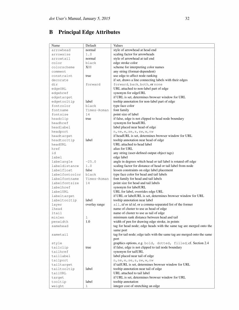
B Principal Edge Attributes

Name Default Valuesarrowhead normal style of arrowhead at head endarrowsize 1.0 scaling factor for arrowheadsarrowtail normal style of arrowhead at tail endcolor black edge stroke colorcolorscheme X11 scheme for interpreting color namescomment any string (format-dependent)constraint true use edge to affect node rankingdecorate if set, draws a line connecting labels with their edgesdir forward forward, back, both, or noneedgeURL URL attached to non-label part of edgeedgehref synonym for edgeURLedgetarget if URL is set, determines browser window for URLedgetooltip label tooltip annotation for non-label part of edgefontcolor black type face colorfontname Times-Roman font familyfontsize 14 point size of labelheadclip true if false, edge is not clipped to head node boundaryheadhref synonym for headURLheadlabel label placed near head of edgeheadport n,ne,e,se,s,sw,w,nwheadtarget if headURL is set, determines browser window for URLheadtooltip label tooltip annotation near head of edgeheadURL URL attached to head labelhref alias for URLid any string (user-defined output object tags)label edge labellabelangle -25.0 angle in degrees which head or tail label is rotated off edgelabeldistance 1.0 scaling factor for distance of head or tail label from nodelabelfloat false lessen constraints on edge label placementlabelfontcolor black type face color for head and tail labelslabelfontname Times-Roman font family for head and tail labelslabelfontsize 14 point size for head and tail labelslabelhref synonym for labelURLlabelURL URL for label, overrides edge URLlabeltarget if URL or labelURL is set, determines browser window for URLlabeltooltip label tooltip annotation near labellayer overlay range all, id or id:id, or a comma-separated list of the formerlhead name of cluster to use as head of edgeltail name of cluster to use as tail of edgeminlen 1 minimum rank distance between head and tailpenwidth 1.0 width of pen for drawing edge stroke, in pointssamehead tag for head node; edge heads with the same tag are merged onto the

same portsametail tag for tail node; edge tails with the same tag are merged onto the same

portstyle graphics options, e.g. bold, dotted, filled; cf. Section 2.4tailclip true if false, edge is not clipped to tail node boundarytailhref synonym for tailURLtaillabel label placed near tail of edgetailport n,ne,e,se,s,sw,w,nwtailtarget if tailURL is set, determines browser window for URLtailtooltip label tooltip annotation near tail of edgetailURL URL attached to tail labeltarget if URL is set, determines browser window for URLtooltip label tooltip annotationweight 1 integer cost of stretching an edge


C Principal Graph Attributes

Name Default Valuesaspect controls aspect ratio adjustmentbgcolor background color for drawing, plus initial fill colorcenter false center drawing on pageclusterrank local may be global or nonecolor black for clusters, outline color, and fill color if fillcolor not definedcolorscheme X11 scheme for interpreting color namescomment any string (format-dependent)compound false allow edges between clustersconcentrate false enables edge concentratorsdpi 96 dots per inch for image outputfillcolor black cluster fill colorfontcolor black type face colorfontname Times-Roman font familyfontnames svg, ps, gd (SVG only)fontpath list of directories to search for fontsfontsize 14 point size of labelid any string (user-defined output object tags)label any stringlabeljust centered ”l” and ”r” for left- and right-justified cluster labels, respectivelylabelloc top ”t” and ”b” for top- and bottom-justified cluster labels, respectivelylandscape if true, means orientation=landscapelayers id:id:id...layersep : specifies separator character to split layersmargin .5 margin included in page, inchesmindist 1.0 minimum separation between all nodes (not dot)nodesep .25 separation between nodes, in inches.nojustify false if true, justify to label, not graphordering if out out edge order is preservedorientation portrait if rotate is not used and the value is landscape, use landscape

orientationoutputorder breadthfirst or nodesfirst, edgesfirstpage unit of pagination, e.g. "8.5,11"pagedir BL traversal order of pagespencolor black color for drawing cluster boundariespenwidth 1.0 width of pen for drawing boundaries, in pointsperipheries 1 number of cluster boundariesrank same, min, max, source or sinkrankdir TB LR (left to right) or TB (top to bottom)ranksep .75 separation between ranks, in inches.ratio approximate aspect ratio desired, fill or autominimizationrotate If 90, set orientation to landscapesamplepoints 8 number of points used to represent ellipses and circles on output (cf.

Appendix Fsearchsize 30 maximum edges with negative cut values to check when looking for a

minimum one during network simplexsize maximum drawing size, in inchessplines draw edges as splines, polylines, linesstyle graphics options, e.g. filled for clustersstylesheet pathname or URL to XML style sheet for SVGtarget if URL is set, determines browser window for URLtooltip label tooltip annotation for clustertruecolor if set, force 24 bit or indexed color in image outputviewport clipping window on outputURL URL associated with graph (format-dependent)


D Graph File Grammar

The following is an abstract grammar for the DOT language. Terminals are shownin bold font and nonterminals in italics. Literal characters are given in singlequotes. Parentheses ( and ) indicate grouping when needed. Square brackets [and ] enclose optional items. Vertical bars | separate alternatives.

graph → [strict] (digraph | graph) id ’{’ stmt-list ’}’stmt-list → [stmt [’;’] [stmt-list ] ]stmt → attr-stmt | node-stmt | edge-stmt | subgraph | id ’=’ idattr-stmt → (graph | node | edge) attr-listattr-list → ’[’ [a-list ] ’]’ [attr-list]a-list → id ’=’ id [’,’] [a-list]node-stmt → node-id [attr-list]node-id → id [port]port → port-location [port-angle] | port-angle [port-location]port-location → ’:’ id | ’:’ ’(’ id ’,’ id ’)’port-angle → ’@’ idedge-stmt → (node-id | subgraph) edgeRHS [attr-list]edgeRHS → edgeop (node-id | subgraph) [edgeRHS]subgraph → [subgraph id] ’{’ stmt-list ’}’ | subgraph id

An id is any alphanumeric string not beginning with a digit, but possibly in-cluding underscores; or a number; or any quoted string possibly containing escapedquotes.

An edgeop is -> in directed graphs and -- in undirected graphs.The language supports C++-style comments: /* */ and //.Semicolons aid readability but are not required except in the rare case that a

named subgraph with no body immediate precedes an anonymous subgraph, be-cause under precedence rules this sequence is parsed as a subgraph with a headingand a body.

Complex attribute values may contain characters, such as commas and whitespace, which are used in parsing the DOT language. To avoid getting a parsingerror, such values need to be enclosed in double quotes.


E Plain Output File Format (-Tplain)

The “plain” output format of dot lists node and edge information in a simple, line-oriented style which is easy to parse by front-end components. All coordinates andlengths are unscaled and in inches.The first line is:

graph scalefactor width heightThe width and height values give the width and the height of the drawing; thelower-left corner of the drawing is at the origin. The scalefactor indicates howmuch to scale all coordinates in the final drawing.The next group of lines lists the nodes in the format:

node name x y xsize ysize label style shape color fillcolorThe name is a unique identifier. If it contains whitespace or punctuation, it isquoted. The x and y values give the coordinates of the center of the node; the widthand height give the width and the height. The remaining parameters provide thenode’s label, style, shape, color and fillcolor attributes, respectively.If the node does not have a style attribute, "solid" is used.The next group of lines lists edges:

edge tail head n x1 y1 x2 y2 . . . xn yn [ label lx ly ] style colorn is the number of coordinate pairs that follow as B-spline control points. If theedge is labeled, then the label text and coordinates are listed next. The edge de-scription is completed by the edge’s style and color. As with nodes, if astyle is not defined, "solid" is used.The last line is always:

stop


F Attributed DOT Format (-Tdot)

This is the default output format. It reproduces the input, along with layout infor-mation for the graph. Coordinate values increase up and to the right. Positionsare represented by two integers separated by a comma, representing the X and Ycoordinates of the location specified in points (1/72 of an inch). A position refersto the center of its associated object. Lengths are given in inches.

A bb attribute is attached to the graph, specifying the bounding box of thedrawing. If the graph has a label, its position is specified by the lp attribute.

Each node gets pos, width and height attributes. If the node is a record,the record rectangles are given in the rects attribute. If the node is polygonaland the vertices attribute is defined in the input graph, this attribute containsthe vertices of the node. The number of points produced for circles and ellipses isgoverned by the samplepoints attribute.

Every edge is assigned a pos attribute, which consists of a list of 3n + 1locations. These are B-spline control points: points p0, p1, p2, p3 are the first Bezierspline, p3, p4, p5, p6 are the second, etc. Currently, edge points are listed top-to-bottom (or left-to-right) regardless of the orientation of the edge. This may change.

In the pos attribute, the list of control points might be preceded by a startpoint ps and/or an end point pe. These have the usual position representation with a"s," or "e," prefix, respectively. A start point is present if there is an arrow at p0.In this case, the arrow is from p0 to ps, where ps is actually on the node’s boundary.The length and direction of the arrowhead is given by the vector (ps− p0). If thereis no arrow, p0 is on the node’s boundary. Similarly, the point pe designates anarrow at the other end of the edge, connecting to the last spline point.

If the edge has a label, the label position is given in lp.


G Layers

dot has a feature for drawing parts of a single diagram on a sequence of overlapping“layers.” Typically the layers are overhead transparencies. To activate this feature,one must set the top-level graph’s layers attribute to a list of identifiers. A nodeor edge can then be assigned to list of layers using its layer attribute. A listof layers is specified as a comma-separated list of ranges, and a range is either asingle layer or has the form id:id’, the latter denoting all layers from id through id’.all is a reserved name for all layers (and can be used at either end of a range, e.gdesign:all or all:code). For example:

layers = "spec:design:code:debug:ship";node90 [layer = "code"];node91 [layer = "design:debug"];node92 [layer = "all:code"];node93 [layer = "spec:code,ship"];node90 -> node91 [layer = "all"];

In this graph, node91 is in layers design, code and debug, while node92 isin layers spec, design and code. node93 is in layers layers spec, design,code and ship.

In a layered graph, if a node or edge has no layer assignment, but incidentedges or nodes do, then its layer specification is inferred from these. To change thedefault so that nodes and edges with no layer appear on all layers, insert near thebeginning of the graph file:

node [layer=all];edge [layer=all];

When PostScript output is selected, the color sequence for layers is set in thearray layercolorseq. This array is indexed starting from 1, and every ele-ment must be a 3-element array which can interpreted as a color coordinate. Theadventurous may learn further from reading dot’s PostScript output.


H Node Shapes

These are the principal node shapes. A more complete description of node shapescan be found at the web site

www.graphviz.org/doc/info/shapes.html

box polygon ellipse circle

plaintext

point egg triangle plaintext

diamond trapezium parallelogram house

hexagon octagon doublecircle doubleoctagon

tripleoctagon invtriangle invtrapezium invhouse

none

Mdiamond Msquare Mcircle none1

2

3

231

32

1

2

3

231

32

record Mrecord


I Arrowhead Types

These are some of the main arrowhead types. A more complete description of theseshapes can be found at the web site

www.graphviz.org/doc/info/arrows.html

normal dot inv

crow tee vee

diamond none box

curve icurve

Arrowhead descriptions support a simple grammar to allow more complex, derivedshapes, such as the examples below.

odot invdot invodot

The web page cited above describes this grammar in detail.


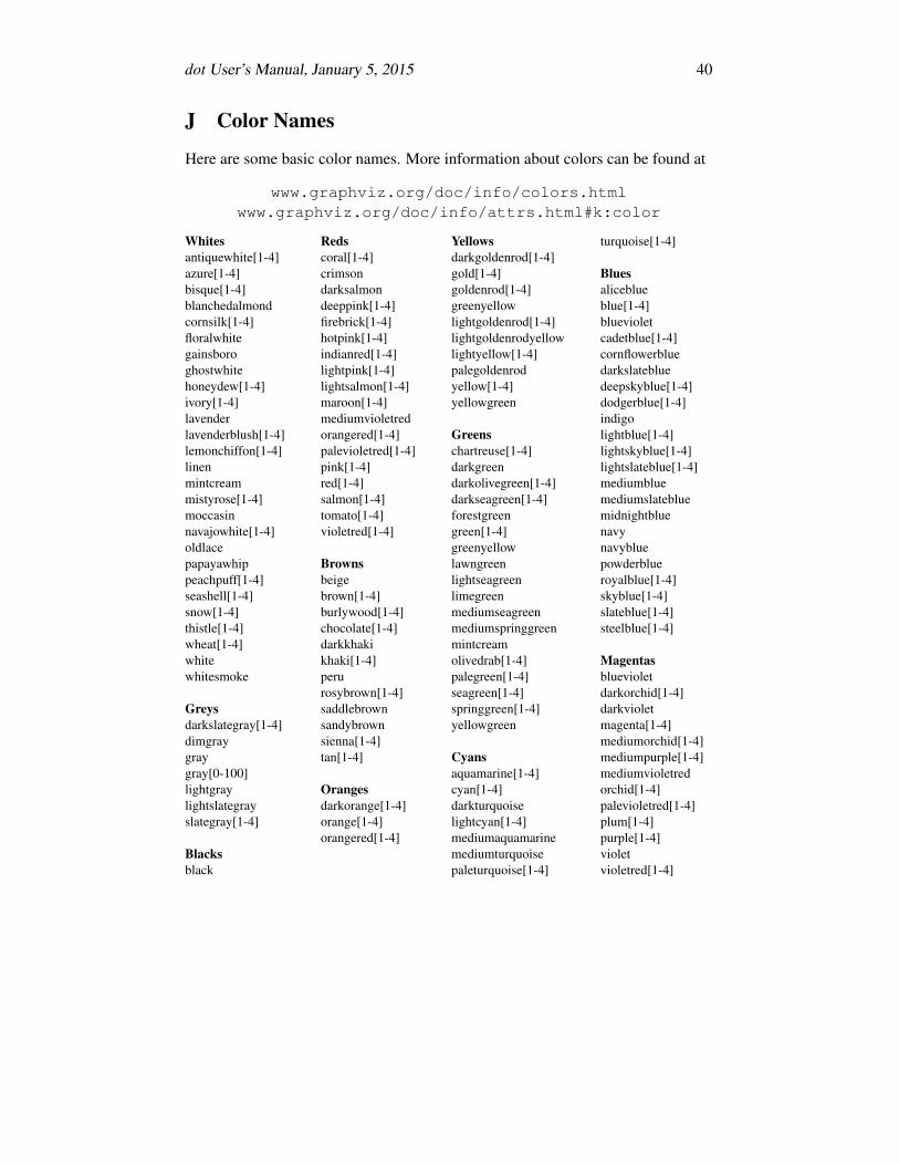
J Color Names

Here are some basic color names. More information about colors can be found at

www.graphviz.org/doc/info/colors.htmlwww.graphviz.org/doc/info/attrs.html#k:color

Whites Reds Yellows turquoise[1-4]antiquewhite[1-4] coral[1-4] darkgoldenrod[1-4]azure[1-4] crimson gold[1-4] Bluesbisque[1-4] darksalmon goldenrod[1-4] aliceblueblanchedalmond deeppink[1-4] greenyellow blue[1-4]cornsilk[1-4] firebrick[1-4] lightgoldenrod[1-4] bluevioletfloralwhite hotpink[1-4] lightgoldenrodyellow cadetblue[1-4]gainsboro indianred[1-4] lightyellow[1-4] cornflowerblueghostwhite lightpink[1-4] palegoldenrod darkslatebluehoneydew[1-4] lightsalmon[1-4] yellow[1-4] deepskyblue[1-4]ivory[1-4] maroon[1-4] yellowgreen dodgerblue[1-4]lavender mediumvioletred indigolavenderblush[1-4] orangered[1-4] Greens lightblue[1-4]lemonchiffon[1-4] palevioletred[1-4] chartreuse[1-4] lightskyblue[1-4]linen pink[1-4] darkgreen lightslateblue[1-4]mintcream red[1-4] darkolivegreen[1-4] mediumbluemistyrose[1-4] salmon[1-4] darkseagreen[1-4] mediumslatebluemoccasin tomato[1-4] forestgreen midnightbluenavajowhite[1-4] violetred[1-4] green[1-4] navyoldlace greenyellow navybluepapayawhip Browns lawngreen powderbluepeachpuff[1-4] beige lightseagreen royalblue[1-4]seashell[1-4] brown[1-4] limegreen skyblue[1-4]snow[1-4] burlywood[1-4] mediumseagreen slateblue[1-4]thistle[1-4] chocolate[1-4] mediumspringgreen steelblue[1-4]wheat[1-4] darkkhaki mintcreamwhite khaki[1-4] olivedrab[1-4] Magentaswhitesmoke peru palegreen[1-4] blueviolet

rosybrown[1-4] seagreen[1-4] darkorchid[1-4]Greys saddlebrown springgreen[1-4] darkvioletdarkslategray[1-4] sandybrown yellowgreen magenta[1-4]dimgray sienna[1-4] mediumorchid[1-4]gray tan[1-4] Cyans mediumpurple[1-4]gray[0-100] aquamarine[1-4] mediumvioletredlightgray Oranges cyan[1-4] orchid[1-4]lightslategray darkorange[1-4] darkturquoise palevioletred[1-4]slategray[1-4] orange[1-4] lightcyan[1-4] plum[1-4]

orangered[1-4] mediumaquamarine purple[1-4]Blacks mediumturquoise violetblack paleturquoise[1-4] violetred[1-4]

drawing graphs with - graphviz

Documents