Computer Science – Research and Development manuscript No.(will be inserted by the editor)

Alexander Wolff

Drawing Subway Maps: A Survey

Received: July 9, 2007 / Revised: November 5, 2007 / DOI: 10.1007/s00450-007-0036-y

Abstract This paper deals with automating the draw-ing of subway maps. There are two features of schematicsubway maps that make them different from drawingsof other networks such as flow charts or organigrams.First, most schematic subway maps use not only hori-zontal and vertical lines, but also diagonals. This givesmore flexibility in the layout process, but it also makesthe problem provably hard. Second, a subway map repre-sents a network whose components have geographic loca-tions that are roughly known to the users of such a map.This knowledge must be respected during the search for aclear layout of the network. For the sake of visual claritythe underlying geography may be distorted, but it mustnot be given up, otherwise map users will be hopelesslyconfused.

In this paper we first give a rather generally acceptedlist of rules that should be adhered to by a good subwaymap. Next we survey three recent methods for draw-ing subway maps, analyze their performance with re-spect to the above rules, and compare the resulting mapsamong each other and to official subway maps drawn bygraphic designers. We then focus on one of the methods,which is based on mixed-integer linear programming, awidely-used global optimization technique. This methodguarantees to find a drawing that fulfills a subset of theabove-mentioned rules (if such a drawing exists) and op-timizes a weighted sum of costs that correspond to theremaining rules. The method can draw even large sub-way networks such as the London Underground in anaesthetically pleasing manner, similar to maps made byprofessional graphic designers. If station labels are in-cluded in the optimization process, so far only medium-size networks can be drawn. Finally we give evidence whydrawing good subway maps is difficult (even without la-bels).

Work supported by grant WO 758/4-2 of the German Re-search Foundation (DFG).

Faculteit Wiskunde en Informatica, Technische UniversiteitEindhoven, Postbus 513, 5600 MB Eindhoven, the Nether-lands, WWW: http://www.win.tue.nl/˜awolff

Keywords Graph drawing · Graph labeling · Subwaymap · Octilinear layout · Mixed-integer program ·NP-hard

Mathematics Subject Classification (2000) 05C62 ·90C90 · 68Q17

1 Introduction

A subway map is a schematic drawing of the underlyinggeographic network that represents the different stationsand subway lines of a subway system. Its purpose is toease navigation in the network for passengers. Passen-gers want to quickly answer questions like: How do I getfrom A to B? Where do I have to change trains? Howmany stops are left? Where to get off? Exact geogra-phy is not only unnecessary for answering these kinds ofquestions, it can be even hindering. This fact has firstbeen discovered and exploited by Harry Beck, an engi-neering draftsman, who created the first schematic mapof the London Underground in 1933. This map and thefate of Harry Beck are interesting stories in their ownright. Garland has devoted a book to them [14], whichis very worth reading. Beck designed his map accord-ing to a simple set of rules: Meandering transport linesare straightened and restricted to horizontals, verticals,and diagonals at 45◦ (we will call such a layout octi-linear). The scale in crowded downtown areas is largerthan in less dense suburbs in order to create more uni-form distances between adjacent stations. In spite of alldistortion, the network topology and a general sense ofthe geometry, e.g., a certain relative position betweensubway stations, is retained. These principles also ap-ply to the majority of contemporary, manually designedsubway maps [21, 26].

A transport network can naturally be represented asa graph, where vertices correspond to stations and edgescorrespond to physical connections between the incidentstations. The true location of stations and tracks deter-mines the input layout of the network. This layout is

2 Alexander Wolff

usually planar (otherwise it can be planarized by intro-ducing dummy vertices at junctions) and hence defines atopological input embedding by specifying for each ver-tex the clockwise order of all adjacent vertices. A lay-out algorithm basically needs to find vertex positions inthe plane such that some desired aesthetic criteria arefulfilled or optimized, e.g., the final drawing should pre-serve the input topology or have few bends along theindividual subway lines, and roughly preserve the inputgeometry. Since subway stations must be labeled, a lay-out algorithm for the network also needs to consider thespace that labels require as these labels must neitheroverlap with each other nor with parts of the networklayout.

The notion of a subway map as we discuss it here is aninteresting compromise between schematic road maps [8]where vertex positions are (mostly) fixed and “conven-tional” graph drawing where vertices can go anywhere.The first approach aims at maintaining the user’s mentalmap, the second approach aims at maximizing aesthet-ics, such as symmetry.

Interestingly enough, the layout principles of subwaymaps have not only been used in a geographic setting.Sandvad et al. [29] and Nesbitt [22] use the metro-mapmetaphor as a way to visualize abstract information re-lated to the Internet and “trains of thoughts”, respec-tively. The metro-map metaphor has inspired artists andhas been used in advertisement, see Figures 1 and 2,respectively, for particularly nice examples. Stott etal. [32] present a prototype tool to draw project plansin a subway-map style. Technical and engineering appli-cations of schematic graph layouts, which are currentlypredominated by orthogonal layouts, can also take ad-vantage of octilinear graph drawing. The main benefit ofoctilinear layouts is that they potentially use less spaceand fewer bends while still being very tidy. For exam-ple in VLSI design the X Architecture [36] is a recenteffort for producing octilinear chip layouts. A differentapplication is to compute schematic layouts of sketchesof graphs, a concept introduced by Brandes et al. [7]. Asketch can be handmade or the physical embedding ofa geometric network like the real position of telephonecables. Brandes et al. give an efficient algorithm for com-puting an orthogonal drawing of a sketch. However, theiralgorithm cannot be extended to more than four direc-tions. This is another possible application area for meth-ods that can draw subway-style maps.

Overview. This article is structured as follows.First, we give a rather generally accepted list of rules

that should be adhered to by a good subway map, seeSection 2.

The main contribution of this article is a survey ofthree methods for drawing subway maps that have re-cently been suggested. All of them rely on some under-lying optimization machinery, which is tuned in order toget drawings that fulfill the above rules as best as possi-

Fig. 1: Poster for the Tate Gallery.

ble. The first of the three methods, by Hong et al. [15],is based on a spring embedder, a force-directed graph-layout method. The attracting and repelling forces thatdrive the movement of the vertices stem from a physicalmodel. They are computed incrementally by a simulated-annealing-like local-optimization algorithm. The secondmethod, by Stott and Rodgers [30], uses multi-criteriaoptimization based on hill climbing, a popular general-purpose local-optimization technique. The third method,by Nollenburg and Wolff [25], relies on mixed-integer pro-gramming, a widely used global-optimization technique.Mixed-integer programming is very powerful, but careneeds to be taken to avoid long running times. We ana-lyze the performance of the three methods with respectto the above list of rules and compare their output ata benchmark (the CityRail network of Sydney) that hasbeen tested by all of them.

Next we focus on the method based on mixed-integerprogramming [25] since it is the only method that guar-antees octilinearity, which, in our opinion, is essentialfor a clear layout of subway maps, see Section 4. It is

Drawing Subway Maps: A Survey 3

Fig. 2: Open source product lines of the publisher O’Reilly. Interchange stations represent books that simultaneously belongto two product lines.

also the first method dedicated to drawing subway mapsthat uses global optimization and thus avoids gettingtrapped in local minima. This contrasts with the othertwo methods based on local optimization. However, sinceno fast algorithm for solving general mixed-integer pro-grams (MIPs) is known, we sketch some heuristic datareduction and speed-up methods, which are importantfor solving larger instances. We also sketch how to ex-tend the basic MIP to combine graph drawing with theplacement of non-overlapping station labels.

This combined discipline has been called graph label-ing by Klau and Mutzel [17]. Klau and Mutzel [17] andBinucci et al. [6] have used MIP formulations for graphlabeling before. However, their methods follow Tamas-sia’s topology-shape-metrics approach [34], which is a com-mon approach for drawing graphs orthogonally. The ap-proach consists of three steps: planarization, orthogonal-ization, and compaction. The first step fixes the embed-ding, the second step its shape (for each edge the se-quence of its bends and their angles is determined), andthe third step the coordinates of the vertices and thebends. Tamassia [34] mentions that his approach for or-

thogonal graph drawing carries over to hexagonal (i.e.,60◦-) drawings, but that the third step fails for drawingswith smaller angles (such as 45◦ in the case of octilineardrawings).

As a justification for the use of the heavy-weight MIPmachinery, we then give Nollenburg’s beautiful proof [24]of the NP-hardness of a restricted version of the subway-layout problem, namely deciding whether a given embed-ded graph can be drawn using straight octilinear edges.The proof reminds of the mechanical constructions thatboys used to build with a Meccano or Marklin modelconstruction kit, see Section 5. The hardness of octilineargraph drawing is in sharp contrast to orthogonal graphdrawing, which Tamassia [34] showed to be efficientlysolvable by his topology-shape-metrics approach.

We conclude with some thoughts about the remain-ing differences between hand- and machine-made subwaymaps, and give an open problem in Section 6.

Before turning to our list of rules for good subwaymaps, we refer the interested reader to a very nicely writ-ten general-audience (German) newspaper article [27]

4 Alexander Wolff

about the drawing of subway networks. It includes someinteresting historic notes.

2 Rules

In this section we list and motivate rules that a goodsubway map should adhere to. Each of the rules is eitherimplicit or explicit in at least two of the papers of Honget al. [15], Stott and Rodgers [30], and Nollenburg andWolff [25], whose algorithms we will discuss in the nextsection. The reader is invited to study the book of Oven-den [26], which contains an abundance of subway mapsfrom all over the world, in order to make up his ownmind as to which set of rules is the right one. It is an in-teresting cartographic question whether the rules behindexisting subway maps are in fact the most user-friendlychoices. For example it is hard to estimate distances ortravel times in a subway map. Pairs of stations with thesame distance in the subway map might actually be sev-eral kilometers apart in peripheral parts but only a fewhundred meters in the city center. User studies oughtto be made in order to evaluate to which extend cur-rent subway maps actually support subway passengersin quickly making the right decisions.

Before listing the rules, we quickly fix some notationroughly following Di Battista et al. [10]. Given a graphG = (V, E) we say that δ is a drawing of G if δ mapseach vertex v of G to a distinct point δ(v) of the planeand each edge {u, v} to a simple (Jordan) curve that con-nects δ(u) and δ(v). A drawing is plane if for any pair ofedges, the corresponding curves have at most endpointsin common. Recall that a graph is planar if it has a planedrawing. A plane drawing partitions the plane into con-nected regions called faces. The unbounded face is alsoreferred to as outer face. An embedding is a useful ab-straction of plane drawings: it fixes the circular orderingof the edges around each vertex and the choice of theouter face. Now we can say that a graph is plane if isplanar and is given with a (plane) embedding.

We assume that we are given a simple plane graph G,to which we refer as the subway graph. We also assumethat we are given a location π(v) ∈ R

2 for each vertexv of G. These locations will usually be the locations ofthe subway stations on a geographic map. (Note that thelocations do not define the embedding since we do notassume that the subway graph has straight-line edges.)

(R1) Keep the input embedding. This supports the men-tal (network) map of the passengers.

(R2) Restrict all line segments to the four octilinear ori-entations horizontal, vertical, and both diagonalsat 45◦. Each orientation has two directions. Thisrestriction makes maps clearer.

(R3) Ensure that adjacent and non-adjacent stations keepa certain minimum distance. This increases thereadability of the map.

(R4) Keep the number of bends along a given subwayline small, especially in interchange stations whereseveral lines meet. If bends cannot be avoided, ob-tuse angles are preferred over acute angles, i.e., theorder of preference is 135◦, 90◦, and 45◦. This rulehelps passengers to follow a subway line with theireyes.

(R5) Preserve the relative position between subway sta-tions. For example, a station being north of someother station in reality should not appear belowthat station on the map. This supports the (geo-graphic) mental map of the passengers.

(R6) Keep the total edge length of the network small.This indirectly makes sure that dense regions ofthe map get a larger share of the available space.Together with rule (R3) this also keeps distancesbetween adjacent stations as uniform as possible.Rule (R6) supports the clarity of the layout.

(R7) Color each edge according to the lines to which itbelongs. This assumes that each line has a uniquecolor. If an edge {u, v} belongs to k lines, thenk copies of that edge (so-called multi-edges) mustbe drawn. Their order along {u, v} should be asconsistent as possible with orders along other edgesincident to u or v. Coloring is essential to help mapusers to follow a line with their eyes.

(R8) Label stations with their names, and make surethat labels do not obscure other labels or partsof the network. Preferably all labels between twointerchange stations are placed on the same side ofthe line; stations on a horizontal line may also bealternatingly labeled above and below the line tosave space. Labels are essential for a readable map.

Clearly, each subway map can only be a compromise ofthe above criteria. For example, a map with a minimumnumber of line bends could drastically distort the mentalmap and, conversely, preserving the mental map couldrequire a large number of bends.

Now we want to state the subway-map layout problemas formally as possible at this point. Let L be a linecover of G, i.e., a set of paths and cycles of G such thateach edge of G belongs to at least one element of L.An element L ∈ L is called a line and corresponds to asubway line of the underlying transport network.

To keep the problem description concise, we do notinsist on coloring (multi-) edges (rule (R7)) and placingstation labels (rule (R8)) for now. Subway lines still playa role when it comes to counting bends, see rule (R4).The ordering of the (line-colored) multi-edges along anedge of G is an interesting research topic by itself and hasfound some attention recently [3, 4]. For more on labelplacement, see Section 4.6.

Problem 1 (Subway-Map Layout Problem) Givena plane graph G = (V, E) with maximum degree 8 andvertex coordinates in R

2, a line cover L of G, find a nicedrawing of G, i.e., a straight-line drawing that followsrules (R1)–(R6) as much as possible.

Drawing Subway Maps: A Survey 5

(a) Geographic layout.

Sydney Harbour

Hawkesbury River

CityCircle

Mountains

Botany Bay

Sydney Suburban Area

Wynyard

Meadowbank

Vineyard

Riverstone

Schofields

Helensburgh

Carin

gbah

Woolo

owar

e

Mira

nda

Cronulla

Wolli Creek

PenshurstMortdaleOatley

ComoJannali

Gym

ea

Loftus

Engadine

Heathcote

ArncliffeBanksia

Carlton

Rockdale

Hurstville

Waterfall

Kirraw

ee

Allawah

Kogarah

Sutherland

Macquarie Fields

Ingleburn

Minto

Leumeah

Macarthur

Campbelltown

Glenfield

Turrel

la

Holsw

orthy

East H

ills

Reves

by

Panan

ia

Padst

ow

River

wood

Nar

wee

Bever

ly H

ills

Kingsg

rove

Bexle

y Nort

h

Bardw

ell P

ark

Tempe Domestic Airport

Mascot

Belm

ore

Wile

y Pa

rk

Punch

bowl

Dulw

ich H

ill

Mar

rickv

ille

Hurls

tone

Park

Cante

rbury

Campsie

Lake

mba

Yagoona

Birrong

Banks

tow

nCabramatta

Warwick Farm

Casula

Liverpool

Leig

htonfie

ld

Cheste

r Hill

Sefton

Carra

mar

Villaw

ood

Yennora

Guildford

Merrylands

Canley Vale

Fairfield

Harris Park

Pendle Hill

Wentworthville

Westmead

Parramatta

Marayong

Doonsid

e

Rooty H

ill

Wer

ringto

n

Kingsw

ood

Toongabbie

Seven Hills

Mount D

ruitt

St M

arys

Quakers Hill

Emu P

lain

s

Penri

th

Berala

Regents Park

Green SquareStan

more

Pete

rsham

Lew

isham

Sum

mer

Hill

Ash

field

Croyd

on

Hom

ebush

Flem

ingto

n

Burwood

Stra

thfiel

d

Clyde

Rosehill

Lidco

mbe

Gra

nville

Auburn

OlympicPark

Camellia Concord West

North Strathfield

Rhodes

Redfern

Town HallSt James

Museum

Kings Cross

Edgecliff

BondiJunction

Martin Place

Milsons PointCircular Quay

North Sydney

Waverton

Artarmon

Wollstonecraft

St LeonardsCarlingford

Telopea

Rydalmere

Dundas

Blacktown

Cheltenham

West Ryde

Denistone

Eastwood

Richmond

East Richmond

Windsor

Mulgrave

Clarendon

Chatswood

Epping

Mac

quarie

Par

k

Mac

quarie

Univ

ersit

y

Nort

h Ryd

e

Gordon

Killara

Roseville

Lindfield

Pennant Hills

Normanhurst

Beecroft

Thornleigh

Hornsby

Wahroonga

Warrawee

Pymble

Turramurra

Waitara

AsquithMount Colah

Mount Kuring-gai

Berowra

Cowan

WKoolewong

Woy Woy

Haw

kesb

ury R

iver

InternationalAirport

New

tow

n

Sydenham

Line under construction

Mac

donaldto

wn

St Peters

Erskineville

Some Southern Highlands servicesoperate directly to and from Central.

Central

South Coast to Southern Highlands*

North Shore and Western Lines

Newcastle & Central Coast Line

Eastern Suburbs & Illawarra Line

(b) Corresponding clipping of the official map [33].

Fig. 3: The Sydney CityRail subway network.

Note that the restriction to graphs with maximumvertex degree 8 is an immediate consequence of the re-striction to octilinear edge directions. Lifting this restric-tion is discussed in the conclusions (Section 6).

3 Methods

There are three recent approaches to automating thedrawing of subway maps. We survey these methods inorder of date of first publication. All of them rely onsome underlying optimization machinery, which is tunedin order to get drawings that fulfill the above rules as bestas possible. The method of Hong et al. [15] is based on aspring embedder, the method of Stott and Rodgers [30]uses hill climbing, and the method of Nollenburg andWolff [25] relies on mixed-integer programming.

As benchmark we use the urban part of the CityRailnetwork of Sydney, a medium-size transportation net-work. The reason for this choice is that the Sydney sub-way graph is the only that appears in all three articles.The fact that our comparison is based on a single networkseems to be rather restrictive. However, when we com-pared for a given method its drawing of our benchmarknetwork to its drawings of other networks, we found thatthe typical features of the method indeed show up in thebenchmark drawing.

Figure 3(a) shows the geographic position of the sta-tions (with straight-line edges connecting them); Fig-ure 3(b) shows the corresponding clipping of the—octi-linear!—official map made by graphic designers. It is in-structive to compare edge lengths in the downtown area(around the station Central) with edge lengths in the

suburbs on each of the two maps. Table 1 describes thecombinatorial size of the network before and after a pre-processing step that is detailed below.

For each method we detail the computing environ-ment used and the running times reported in the cor-responding article. Although the set-ups were of coursenot identical, all methods have been implemented in Javaand were run on single-processor machines with clockrates of 2.2–3 GHz and 0.5–4 GB RAM. Thus it is likelythat a running time in the order of seconds or minuteson one machine would have remained of the same orderon another. One can argue that running time is not crit-ical when drawing subway maps that usually have a lifeexpectancy of several years. However, if the new meth-ods for octilinear drawing are to challenge conventionalmethods for orthogonal drawing (of class diagrams insoftware projects, for example), then speed may becomemore important than aesthetics. Certain use cases, suchas on-line mapping, are ruled out by methods that usu-ally need more than a few seconds to produce a result.

G n m m′ f

original 174 183 289 11

contracted [15] 31 40 40 11

contracted [25] 67 76 145 11

Table 1: Numbers n, m, m′, and f of vertices, edges, multi-edges, and faces of the Sydney subway graph, respectively.

6 Alexander Wolff

(a) Complete unlabeled map. (b) Clipped labeled map [15]. The clipping corresponds tothe maps in Figure 3.

Fig. 4: Drawings of the Sydney CityRail network by Hong et al.

3.1 Spring embedder

The first method, by Hong et al. [15], is based on a springembedder. A spring embedder is an iterative algorithmthat simulates a physical system that in turn representsthe graph to be drawn. One can think of the verticesas particles with repelling forces and of the edges assprings with contracting forces. This very popular andfast all-round graph-drawing algorithm was suggested byFruchterman and Reingold [12] in the early 1990’s.

There are plenty of spring-embedder variants avail-able. One of them is PrEd [5], which Hong et al. chose asbasis of their algorithm since PrEd maintains the embed-ding of the input graph. Hong et al. give five algorithmsto address the subway-map layout problem. The mostrefined of these algorithms modifies PrEd such that edgeweights are taken into account and such that additionalmagnetic forces draw the straight-line edges towards theclosest octilinear direction. As in the original version ofPrEd, the total force acting on a vertex is simply the sumof all attracting and repelling forces that act on that ver-tex. Some of the expressions for the partial forces includemodel-tuning parameters; the authors mention seven forthe x-components of the partial forces alone.

Hong et al. consider the geometry of the input net-work only implicitly: they use the original embeddingas initial layout. In a preprocessing step they simplifythe subway graph by collapsing all degree-2 vertices. See

Table 1 for the effect of this. Then they set the weightof each edge e in the remaining graph to the numberof original edges that e replaces. Having computed thefinal layout, Hong et al. re-insert all degree-2 verticesinto the corresponding edges in an equidistant manner.Their algorithm is very fast: all their examples were com-puted within a few seconds on a single-processor 3.0 GHzPentium-4 machine with 1 GB of RAM under the SunMicrosystems Java-2 Runtime Environment, StandardEdition. The Sydney CityRail network with fixed em-bedding took 7.6 seconds. Station labels are placed in asecond, independent step. While label–label overlaps areavoided, labels sometimes do intersect edges.

Figure 4(b) is a clipping of Figure 17 in the article ofHong et al. [15] and shows their Sydney CityRail map.Originally they draw a slightly larger labeled network(for the unlabeled counterpart, see Figure 4(a)), wherelines extend further into the suburbs, but we only con-sider the part corresponding to the graph in Figure 3(a).If the depicted drawing is to be judged with respect tothe rules (R1)–(R6), it is clear that the drawing pre-serves the embedding, i.e., (R1) is fulfilled by construc-tion. It further seems that relative position (rule (R5))is respected quite well. This is probably due to the factthat the geographic layout was the starting point of theiterative layout process. On the other hand one can ob-serve that edges are not strictly octilinear (R2) and thatthere is a large variance in the distribution of the edge

Drawing Subway Maps: A Survey 7

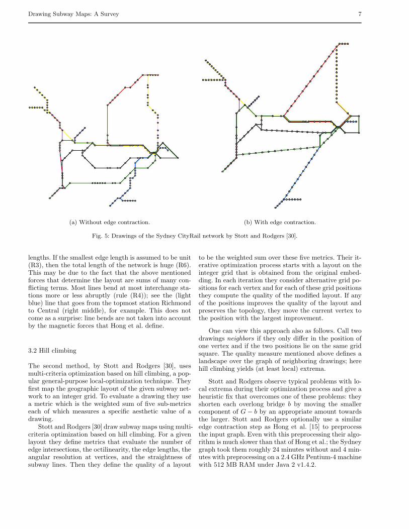
(a) Without edge contraction. (b) With edge contraction.

Fig. 5: Drawings of the Sydney CityRail network by Stott and Rodgers [30].

lengths. If the smallest edge length is assumed to be unit(R3), then the total length of the network is huge (R6).This may be due to the fact that the above mentionedforces that determine the layout are sums of many con-flicting terms. Most lines bend at most interchange sta-tions more or less abruptly (rule (R4)); see the (lightblue) line that goes from the topmost station Richmondto Central (right middle), for example. This does notcome as a surprise: line bends are not taken into accountby the magnetic forces that Hong et al. define.

3.2 Hill climbing

The second method, by Stott and Rodgers [30], usesmulti-criteria optimization based on hill climbing, a pop-ular general-purpose local-optimization technique. Theyfirst map the geographic layout of the given subway net-work to an integer grid. To evaluate a drawing they usea metric which is the weighted sum of five sub-metricseach of which measures a specific aesthetic value of adrawing.

Stott and Rodgers [30] draw subway maps using multi-criteria optimization based on hill climbing. For a givenlayout they define metrics that evaluate the number ofedge intersections, the octilinearity, the edge lengths, theangular resolution at vertices, and the straightness ofsubway lines. Then they define the quality of a layout

to be the weighted sum over these five metrics. Their it-erative optimization process starts with a layout on theinteger grid that is obtained from the original embed-ding. In each iteration they consider alternative grid po-sitions for each vertex and for each of these grid positionsthey compute the quality of the modified layout. If anyof the positions improves the quality of the layout andpreserves the topology, they move the current vertex tothe position with the largest improvement.

One can view this approach also as follows. Call twodrawings neighbors if they only differ in the position ofone vertex and if the two positions lie on the same gridsquare. The quality measure mentioned above defines alandscape over the graph of neighboring drawings; herehill climbing yields (at least local) extrema.

Stott and Rodgers observe typical problems with lo-cal extrema during their optimization process and give aheuristic fix that overcomes one of these problems: theyshorten each overlong bridge b by moving the smallercomponent of G − b by an appropriate amount towardsthe larger. Stott and Rodgers optionally use a similaredge contraction step as Hong et al. [15] to preprocessthe input graph. Even with this preprocessing their algo-rithm is much slower than that of Hong et al.; the Sydneygraph took them roughly 24 minutes without and 4 min-utes with preprocessing on a 2.4 GHz Pentium-4 machinewith 512 MB RAM under Java 2 v1.4.2.

8 Alexander Wolff

For the results, see the maps in Figure 5. These mapsfulfill most of our rules quite well. Rule (R4) is one ofthe exceptions; especially in Figure 5(a) there are manyunnecessary bends, but also in Figure 5(b) most linesbend in most interchange stations. Again, take the (hereyellow) line from Richmond to Central as an example.Recall that one of the five metrics that Stott and Rodgersuse to define the quality of a layout in fact punishes thenumber of bends. Increasing the weight of this metricwould probably yield a map with fewer bends—maybeat the expense of the other metrics.

There seems to be an interesting trade-off betweenrules (R2) and (R6): the map that was drawn withoutthe edge-contraction step (Figure 5(a)) contains only onenon-octilinear edge, but a rather high variance of edgelengths, while the other map (Figure 5(b)) has three non-octilinear paths of degree-2 vertices, but more or lessuniform edge lengths (due to the edge-contraction step).

The first of their five metrics punishes intersections,which means that a non-plane drawing can become planeduring the layout process. This is what happened to theintersection between the city circle and the blue line—the last three stations which actually lie outside the circle(see the rightmost stations in Figures 3(b) versus those inFigure 5) are moved inside. The idea behind this metric isthat it should remove intersections that may sometimescome into being since the initial layout uses geographicstation positions and straight-line edges. However, in theSydney example it would probably have made sense todo the obvious: insert a dummy vertex at the intersectionand call the layout algorithm (possibly punishing bendsat dummy vertices harder). This approach may result inunwanted bends (at points other than stations), but atleast the network topology would be correct.

Stott and Rodgers [31] extend their previous methodby integrating station labeling into their optimizationprocess. After each iteration of vertex movements thenumber of intersections between labels and edges, ver-tices, and other labels is minimized. In spite of this,they experience quite a few label–label overlaps, espe-cially along horizontal edges. The authors do not giveinformation on the running time of their method for la-beled subway maps. The networks they draw and labelare rather small (at most five lines) and, more impor-tantly, have few faces (one to three, including the outerface).

3.3 Mixed-integer programming

The third method, by Nollenburg and Wolff [25], is basedon mixed-integer linear programming, a widely used global-optimization technique. A mixed-integer linear program(MIP) consists of (a) integer and real variables, (b) a lin-ear objective function, i.e., a weighted sum of the vari-ables, and (c) linear constraints, i.e., equalities or in-equalities that have a weighted sum of the variables on

one side and a constant on the other. In contrast to linearprogramming, where integer variables are not allowed,mixed-integer programming is very versatile and can beused to model many problems. Since this includes NP-hard problems, no polynomial-time algorithm for generalMIPs is known. However, there is a number of public-domain (e.g., lp solve) and commercial solvers available(e.g., CPLEX). The size of the instances that these pro-grams can solve and the resulting running times dependheavily on the problem. However, even if it may take along time to solve a MIP to optimality, a MIP solver usu-ally finds better and better feasible solutions in the pro-cess, i.e., solutions that fulfill all (integrality and other)constraints, but which may not be optimal. This is ofinterest for practical problems such as the drawing ofsubway maps, where optimality is often not required.Moreover, with each feasible solution MIP solvers outputa so-called optimality gap, i.e., the relative gap betweenthe cost of the feasible solution and the best lower boundcurrently proven by the MIP solver. This is a valuablequality estimate.

Nollenburg and Wolff [25] model the problem by split-ting the list of rules. They refer to rules (R1)–(R3) ashard constraints and to rules (R4)–(R6) as soft con-straints. The hard constraints are those that Nollenburgand Wolff insisted on, while the soft constraints modelaesthetic criteria that are to be optimized among alldrawings that fulfill the hard constraints. Given thesetwo categories, the hard constraints were translated intolinear equalities and inequalities of a set of variables (ba-sically the coordinates of the vertices). Then the softconstraints were translated into a weighted sum of threecost functions that measure how well these constraintsare fulfilled. These are the ingredients of a MIP formula-tion: variables, linear constraints, and a linear objectivefunction. This translation of rules into a formulation thatonly allows linear expressions is probably the most dif-ficult part of the work, see Section 4.

Given the MIP formulation and a concrete input—the embedding of the input graph, the locations of thevertices, and the line cover—, the corresponding MIPinstance can be generated automatically. Then a MIPsolver is called. If the MIP instance is not too large,the problem not too difficult, and the solution space notempty, the MIP solver will find feasible solutions of bet-ter and better quality and eventually the optimal solu-tion. Note that here a feasible solution corresponds toa drawing that meets all hard constraints, and an opti-mal solution corresponds to a drawing that additionallyoptimizes the soft constraints.

The MIP approach yielded the planar layout in Fig-ure 6(a). Nollenburg and Wolff [25] report a computa-tion time of 22 minutes that was based on a simplead-hoc heuristic for reducing the size of the MIP. Inthe meantime—given some more engineering (see Sec-tion 4.5)—the computation time has been reduced to77 seconds with the MIP solver CPLEX 9.1 running on

Drawing Subway Maps: A Survey 9

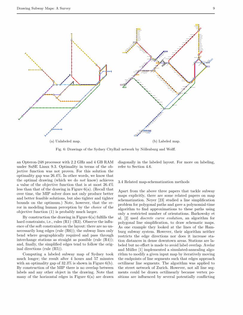
(a) Unlabeled map.

Wyn

yard

Regents Park

St James

Casula

Kings C

ross

Edgec

liff

Bondi

Junc

tion

Berala

Blacktown

Sydenham

North

Syd

ney

Town

Hall

Sutherland

Waverton

Wollstonecraft

St Leonards

Artarmon

Chatswood

Roseville

Lindfield

Killara

Gordon

Pymble

Turramurra

Warrawee

Wahroonga

Waitara

Yagoona

Bankstown

Punchbowl

Wiley Park

Lakemba

Belmore

Campsie

Canterbury

Hurlstone Park

Dulwich Hill

Marrickville

Olympic

Par

k Milsons Point

Liverpool

Cabramatta

Central

Birron

g

Asquith

Mt Colah

Mt Kuring-gai

Berowra

Harris Park

Lidcombe

Auburn

Sefto

n

Tempe

Burwood

Croydon

Ashfield

Summer Hill

Lewisham

Petersham

Stanmore

Newtown

Macdonaldtown

North Strathfield

Concord West

Rhodes

Meadowbank

West Ryde

Denistone

Eastwood

Epping

Cheltenham

Beecroft

Pennant Hills

Thornleigh

Normanhurst

Jannali

Como

Oatley

Mortdale

Penshurst

Hurstville

Allawah

Carlton

Kogarah

Rockdale

Banksia

Arncliffe

Homeb

ush

Kirraw

ee

Gymea

Mira

nda

Caring

bah

Woo

loowar

e

Cronu

lla

Fleming

ton

Warwick Farm

Mar

tin P

laceGuildford

Yennora

Fairfield

Canley Vale

Loftus

Engadine

Heathcote

Waterfall

Erskineville

St Peters

Horns

by

Clyde

Cheste

r Hill

Leigh

tonf

ield

Villawoo

d

Carra

mar

Holsworthy

East Hills

Panania

Revesby

Padstow

Riverwood

Narwee

Beverly Hills

Kingsgrove

Bexley North

Bardwell Park

Turrella

Macquarie Fields

Ingleburn

Minto

Leumeah

Wolli Creek

Macarthur

Circular Quay

Strath

field

Glenfield

Marayong

Quakers Hill

Schofields

Riverstone

Vineyard

Mulgrave

Windsor

Clarendon

East Richmond

Richmond

Merrylands

Doonside

Rooty Hill

Mt Druitt

St Marys

Werrington

Kingswood

Penrith

Emu Plains

Green Square

Mascot

Domestic

International

Granv

ille

Rosehill

Camellia

Rydalmere

Dundas

Telopea

Carlingford

Redfern

Campbelltown

Parramatta

Westmead

Wentworthville

Pendle Hill

Toongabbie

Seven Hills

Museum

(b) Labeled map.

Fig. 6: Drawings of the Sydney CityRail network by Nollenburg and Wolff.

an Opteron-248 processor with 2.2 GHz and 4 GB RAMunder SuSE Linux 9.3. Optimality in terms of the ob-jective function was not proven. For this solution theoptimality gap was 26.4%. In other words, we know thatthe optimal drawing (which we do not know) achievesa value of the objective function that is at most 26.4%less than that of the drawing in Figure 6(a). (Recall thatover time, the MIP solver does not only produce betterand better feasible solutions, but also tighter and tighterbounds on the optimum.) Note, however, that the er-ror in modeling human perception by the choice of theobjective function (1) is probably much larger.

By construction the drawing in Figure 6(a) fulfills thehard constraints, i.e., rules (R1)–(R3). Observe the influ-ence of the soft constraints on the layout: there are no un-necessarily long edges (rule (R6)); the subway lines onlybend where geographically required and pass throughinterchange stations as straight as possible (rule (R4));and, finally, the simplified edges tend to follow the orig-inal directions (rule (R5)).

Computing a labeled subway map of Sydney tookmuch longer; the result after 4 hours and 57 minuteswith an optimality gap of 32.3% is shown in Figure 6(b).By construction of the MIP there is no overlap betweenlabels and any other object in the drawing. Note thatmany of the horizontal edges in Figure 6(a) are drawn

diagonally in the labeled layout. For more on labeling,refer to Section 4.6.

3.4 Related map-schematization methods

Apart from the above three papers that tackle subwaymaps explicitly, there are some related papers on mapschematization. Neyer [23] studied a line simplificationproblem for polygonal paths and gave a polynomial-timealgorithm to find approximations to these paths usingonly a restricted number of orientations. Barkowsky etal. [2] used discrete curve evolution, an algorithm forpolygonal line simplification, to draw schematic maps.As one example they looked at the lines of the Ham-burg subway system. However, their algorithm neitherrestricts the edge directions nor does it increase sta-tion distances in dense downtown areas. Stations are la-beled but no effort is made to avoid label overlap. Avelarand Muller [1] implemented a simulated-annealing algo-rithm to modify a given input map by iteratively movingthe endpoints of line segments such that edges approachoctilinear line segments. The algorithm was applied tothe street network of Zurich. However, not all line seg-ments could be drawn octilinearly because vertex po-sitions are influenced by several potentially conflicting

10 Alexander Wolff

terms. Ware et al. [35] built on the work of Avelar andMuller and tailor it towards mobile applications withsmall screens. Cabello et al. [8] presented an efficientalgorithm for schematizing road networks. Their algo-rithm draws edges as octilinear paths with two or threelinks and preserves the input topology. However, all ver-tices keep their original positions, which is in generalnot desired for drawing subway maps. Cabello and vanKreveld [9] studied approximation algorithms for align-ing points octilinearly, where each point can be placedanywhere in its own given region. Yet, their method doesnot guarantee to preserve the embedding if points cor-respond to vertices of a graph. Merrick and Gudmunds-son [20] suggested an efficient algorithm that simplifiespolygonal chains using the following criteria. Given apolygonal chain P , a fixed set C of directions, and anaccuracy ε, their algorithm finds a polygonal chain P ′

that is (a) C-oriented, (b) goes through all radius-ε cen-tered at vertices of P in the right order, and (c) has theminimum number of bends among all chains that ful-fill (a) and (b). They apply their algorithm to drawingsubway networks. However, since the algorithm processeseach subway line individually, the input topology is notkept.

4 Mixed-Integer Program

Nollenburg and Wolff formulate the subway-map lay-out problem as a MIP. As we will see in Section 5, thesubway-map layout problem is NP-hard. This is a goodjustification for applying a likewise NP-hard optimiza-tion method such as mixed-integer programming. Theexpressive power of mixed-integer programming gives thenecessary flexibility to achieve the following. If a layoutthat conforms to all hard constraints exists (and this wasthe case in all examples that Nollenburg and Wolff tried),then their MIP finds such a layout. At the same time,their MIP optimizes the weighted sum of cost functionseach of which corresponds to a soft constraint. Before wedescribe a number of features of this MIP we give somebasics on linear programming.

4.1 Basics

A MIP consists of two parts: a set of linear constraintsand a linear objective function. We give a simple two-dimensional example, see Figure 7.

Consider the objective function

maximize x + 2y (1)

subject to the constraints

y ≤ 0.9 · x + 1.5 (2)y ≥ 1.4 · x − 1.3. (3)

c

s∗

s

S

(2)

(3)

x

y

1

1

Fig. 7: Difference between optimal fractional solution s∗ andoptimal integral solution s.

Each constraint corresponds to a halfplane; the intersec-tion of the halfplanes—a (possibly unbounded) polygon—represents the set S of feasible solutions. In Figure 7 thesolution polygon is the shaded region. Among the pointsin S we are interested in one that maximizes the objec-tive function, which also has a geometric interpretation.The coefficients of the variables in the objective functionyield a vector c, here c =

(

12

)

. If we sweep the plane indirection c with a line ℓ orthogonal to c, then the lastpoints of S swept by ℓ are those that maximize (1). Thetraces of ℓ are marked by the dashed lines in Figure 7.

Objective function (1) and constraints (2) and (3)represent in fact a linear program (LP). LPs can besolved efficiently, e.g., by Karmakar’s interior-point me-thod [16]. This changes radically when we add integralityconstraints, e.g.,

x, y ∈ Z. (4)

Then we get an integer (linear) program (IP), whose so-lution set consists of those points in S that lie on theinteger grid. In our example in Figure 7 these points aremarked by black dots. Note that the optimum solution sof the IP (1)–(4) is usually far from the optimum solutions∗ of the LP (1)–(3); the optimum integral solution s cannot be obtained from the optimum fractional solution s∗

by rounding down the components of the vector s∗. AMIP can have both, fractional and integral variables.

Integrality constraints make a continuous problemdiscrete; if the set of fractional solutions is bounded,then the number of integral solutions becomes finite. Soit seems solving the more restricted problem is easier.However, the opposite is the case. Geometric propertiesof the LP that are exploited by efficient solution strate-gies are lost. On the other hand a lot more problems canbe modeled with the help of integer variables.

We give an example that will come in handy lateron, a standard trick in MIP modeling. Suppose we wantto make sure that at least one of three constraints C1,C2, and C3 is fulfilled, but not necessarily all of them.In other words, we want to express the disjunction C1 ∨

Drawing Subway Maps: A Survey 11

C2 ∨ C3. Suppose

C1 : x − 3 ≤ 0,C2 : y ≤ 0,C3 : x + y ≤ 0.

Then we introduce three binary variables α1, α2, andα3, i.e., variables that are restricted to the set {0, 1}. Wefurther restrict these variables by the constraint

α1 + α2 + α3 ≥ 1. (5)

Now we can formulate C1 ∨ C2 ∨ C3 as the conjunctionC′

1 ∧ C′2 ∧ C′

3, where

C′1 : x − 3 ≤ M(1 − α1),

C′2 : y ≤ M(1 − α2),

C′3 : x + y ≤ M(1 − α3).

(6)

and M is a large constant that must be an upper boundon the left-hand sides of the inequalities. Note that (5)and (6) are a conjunction of linear constraints, i.e., legalpart of a MIP. By the way: it is worth making M as tighta bound on the left-hand sides as possible—this helps tospeed up solving the MIP.

4.2 Overview

In the remainder of this section we peek into the MIPformulation of Nollenburg and Wolff [25]. We have chosentwo parts. We first detail how the rather subway-specifichard constraint octilinearity (rule (R2)) is modeled, seeSection 4.3. Then, we turn to the soft constraint relativeposition (rule (R5)), which is also specific to drawinggeometric networks such as subway maps, see Section 4.4.

Recall that Nollenburg and Wolff (roughly) translatethe three hard constraints (R1)–(R3) into the linear con-straints of their MIP, and the three soft constraints (R4)–(R6) into the objective function. The objective functionis simply the weighted sum of three individual cost func-tions:

Minimize λR4 costR4 + λR5 costR5 + λR6 costR6, (7)

where the constants λR4, λR5, and λR6 can be set bythe user. Each of them individually emphasizes a certainaesthetic criterion. The function costR5 responsible foroptimizing relative position is treated in detail in Sec-tion 4.4, for the other two cost functions see [25].

The total number of constraints and variables in theMIP formulation of Nollenburg and Wolff is O(n + m′ +m2), where m′ > m is the sum of the number of edges inall lines in L(counting multiple edges). Note that since Gis planar, Euler’s polyhedral formula yields m ≤ 3n− 6.Section 4.5 deals with methods for reducing the size ofthe subway graph and of the MIP. Section 4.6 describeshow vertex labels can be included in the MIP model.Section 4.7 describes how the speed-up techniques and

x

y

z1

z2

Fig. 8: The octilinear coordinate system with an octilineargrid in the background. The marked points all have the sameL∞-distance from the origin.

the integration of label placement affect running timeand results.

We close this overview by presenting the coordinatesystem that we are going to use. The idea is that wewould like to handle all four edge orientations similarly.Hence we use an (x, y, z1, z2)-coordinate system as de-picted in Figure 8, where each axis corresponds to one ofthe four edge orientations in the layout. For each vertexv ∈ V we set

z1(v) = x(v) + y(v)z2(v) = x(v) − y(v).

(8)

These defining equations are also part of the MIP formu-lation and use real-valued variables for the coordinates.

Furthermore, we need to specify an underlying met-ric for measuring distances. We decided to use the L∞-metric, which defines the distance of two vertices u and vto be max(|x(u)−x(v)|, |y(u)−y(v)|). This metric has thenice property that all points on the boundary of the unitsquare centered at any point p have the same distancefrom p. In Figure 8 eight points on the octilinear coordi-nate axes are shown that all have the same L∞-distancefrom the origin. One side-effect of using the L∞-metricis that all vertices will be placed on a axis-aligned gridas long as all edge lengths in the L∞-metric are integers.Attention needs to be paid because a z1- or z2-coordinatedifference of 2 corresponds to an L∞-distance of 1.

4.3 Enforcing Octilinearity and Relative Position

The following part of the MIP formulation models hardconstraints, namely that all edges are drawn as straight,octilinear line segments with a given minimum length,as stated in rules (R2) and (R3). Note that rule (R3) isonly partially covered here. The distance requirement fornon-adjacent vertices is more naturally handled togetherwith the enforcement of planarity, see [25].

At the same time, the direction of each edge {u, v}in the output drawing is restricted to the three closest

12 Alexander Wolff

u

12

3

4

56

0

7v

Fig. 9: Numbering of the sectors and the octilinear directionsrelative to vertex u, e.g., secu(v) = 5.

octilinear approximations1 of the line segment π(u)π(v)specified by the input. Hence, the soft constraint (R5)is partially modeled as a hard constraint, too. Relativeposition can also be modeled completely as a soft con-straint, but excluding a number of directions has thepotential of speeding up the solving of the MIP.

Before formulating the constraints we need some no-tation to address relative positions between vertices andto denote directions of edges. For technical reasons wedirect all edges arbitrarily. If we write an edge as uv, wemean that it is directed from u to v. For each vertex uwe define a partition of the plane into eight sectors. Eachsector is a 45◦-wedge with apex u. The wedges are cen-tered around rays that emanate from u and follow oneof the four orientations either in positive or in negativedirection. The sectors are numbered from 0 to 7 coun-terclockwise starting with the positive x-direction, seeFigure 9.

To denote the rough relative position between twovertices u and v in the original layout we use the termssecu(v) and secv(u) representing the sector relative tou in which v lies and vice versa. Note that these termsare known before solving a concrete instance and arethus constants from the MIP point of view. For eachedge uv, we introduce the variable dir(u, v) to denote theoctilinear direction of uv in the new layout. We identifyeach octilinear direction with its corresponding sector.For example if edge uv leaves u in negative z1-direction,we say dir(u, v) = 5. To make the difference betweensecu(v) and dir(u, v) really clear, note that the formerdescribes the (known) input, while the latter describesthe (unknown) output. Both fulfill a kind of symmetry:

secu(v) = secv(u) + 4 (mod 8) anddir(u, v) = dir(v, u) + 4 (mod 8).

As mentioned above, we partially model the soft con-straint (R5) as a hard constraint. As a compromise be-tween conservation of relative positions and flexibility toobtain a nice drawing, we allow that an edge is drawnin one of three different ways. It can be drawn in thedirection corresponding to its original sector relative to

1 This means that the angle between the directed linesthrough u and v in in- and output is at most 67.5◦.

either endpoint or it can be drawn in the two neighboringdirections. Let

secpredu (v) = secu(v) − 1 (mod 8),

secorigu (v) = secu(v),

secsuccu (v) = secu(v) + 1 (mod 8).

Recall that secu(v) is a constant, thus secpredu etc. are

also constants, and there is no need to perform modulooperations in the MIP.

We now restrict dir(u, v) (which is also used in otherparts of the MIP formulation, e.g., in Section 4.4) to theset {secpred

u (v), secorigu (v), secsucc

u (v)}. For example, in thesituation depicted in Figure 9, we want that dir(u, v) ∈{4, 5, 6}. At the same time we must make sure that thevalues of dir(u, v) and dir(v, u) correspond to oppositedirections. This is expressed by the disjunction

(dir(u, v) = secpredu (v) ∧ dir(v, u) = secpred

v (u)) ∨(dir(u, v) = secorig

u (v) ∧ dir(v, u) = secorigv (u)) ∨

(dir(u, v) = secsuccu (v) ∧ dir(v, u) = secsucc

v (u)).

(9)

To model disjunction (9) we apply the first half of thestandard trick that we detailed in Section 4.1: we intro-duce binary variables αpred(u, v), αorig(u, v), αsucc(u, v),and the constraint

αpred(u, v) + αorig(u, v) + αsucc(u, v) = 1 (10)

for each edge uv ∈ E. The (unique) variable that takesvalue 1 in (10) will determine the part of disjunction (9)that evaluates to true and thus the direction in whichedge uv is drawn. Now the following constraint definesdir(u, v).

dir(u, v) =∑

i∈{pred,orig,succ} seciu(v) · αi(u, v) (11)

Here the unique variable αi(u, v) that equals 1 selectsthe sector seci

u(v) that is assigned to dir(u, v). Note thatthe constraint is indeed linear since seci

u(v) is a constant.The constraint for dir(v, u) is analogous.

We use the variables of type αi(u, v) not only to de-fine dir(u, v) (which at the same time constrains the rel-ative position of adjacent vertices u and v in the outputdrawing), but we also use the αi’s to enforce octilinear-ity. For example, let secpred

u (v) = 4 as in Figure 9. Thenwe introduce the following constraints for edge uv andi = pred:

y(u) − y(v) ≤ M(1 − αpred(u, v))−y(u) + y(v) ≤ M(1 − αpred(u, v))

x(u) − x(v) ≥ −M(1 − αpred(u, v)) + ℓuv,(12)

where ℓuv > 0 is the minimum length of edge uv accord-ing to rule (R3). Here, we apply the second half of thestandard trick from Section 4.1. In this case the valueof the “large constant” M depends on the coordinaterange. For example, we can set M = n if at the sametime we force the output drawing to lie in the square[0, n]×[0, n]. Observe that constraints (12) are equivalent

Drawing Subway Maps: A Survey 13

to y(u) = y(v) and x(u) ≥ x(v) + ℓuv if αpred(u, v) = 1.This is exactly what is needed for an edge pointing hor-izontally to the left.

The constraints for other edge directions and for thecases i = orig and i = succ are constructed analogously.

4.4 Optimizing Relative Position

To preserve as much of the overall appearance of the sub-way network as possible we have already restricted theedge directions to the set of the three octilinear directionsclosest to the input direction. Ideally, one wants to drawan edge uv using its nearest octilinear approximation,i.e., the direction where dir(u, v) = secu(v). Nollenburgand Wolff model (R5) by introducing a cost of 1 in casethe layout does not use that direction.

For each edge uv they define as its cost a binary vari-able ρ(uv) which is 0 if and only if dir(u, v) = secu(v).This is modeled by

−Mρ(uv) ≤ dir(u, v) − secu(v) ≤ Mρ(uv). (13)

Now the cost for deviating from the original relative po-sitions can simply be expressed as

cost(R5) =∑

uv∈E

ρ(uv). (14)

4.5 Speed-Up Techniques

A common feature of subway maps is that they tend tohave a large number of degree-2 vertices on line sectionsbetween two interchange stations. As we have seen inSection 3, both Hong et al. [15] and Stott and Rodgers [30]contract all degree-2 vertices, define appropriate edgeweights, apply their layout algorithms on the contractedgraph, and then reinsert the degree-2 vertices. Nollen-burg and Wolff [25] modify this data-reduction trick bykeeping up to two dummy vertices on each chain of de-gree-2 vertices. The rationale behind drawing the con-nection between the corresponding interchange verticesas a polyline with at most three segments is that this dis-torts the map less than insisting on no bends. Again, theoriginal vertices are reinserted uniformly on their cor-responding polylines. Nollenburg and Wolff report thattheir experiments showed that this is a good compromisebetween flexibility of the drawing and size of the MIPmodel. Recall that the target function penalizes bendsalong lines so that in many cases bends at these specialdegree-2 vertices are in fact avoided.

The only part of their MIP formulation that needsa quadratic number of constraints (and variables) is theone that ensures planarity, which is a direct consequenceof rule (R3). This is why the most urgent need is to re-duce the number of these constraints. An immediate re-duction is as follows. For a planar drawing of an embed-ded graph it suffices to require that non-incident edges of

the same face do not intersect. This already guaranteesthat no two edges intersect except at common endpoints.So instead of introducing planarity constraints for allpairs of non-incident edges, it is enough to include themonly for pairs of non-incident edges of the same face.

However, the number of these planarity constraints isoften still far too high, see Section 4.7. Nollenburg andWolff observed that, on the one hand, only a small frac-tion of all possible intersections was relevant for the lay-out. On the other hand, it is not clear how to determinerelevant edge pairs in advance. A way out is the callbackfunction of the MIP optimizer CPLEX. Nollenburg andWolff exploit this as follows. Their initial MIP formu-lation does not contain any planarity constraints at all.Then, during the optimization process, planarity con-straints are added on demand as follows. Whenever theoptimizer returns a new (and better) feasible solution,a callback routine is notified. This routine interruptsthe optimizer and checks externally for edge crossingsin the layout that corresponds to the current feasible so-lution. If the layout contains pairs of intersecting edges,Nollenburg and Wolff add only the planarity constraintscorresponding to those pairs and continue the optimiza-tion. If the current layout is plane, it is stored. The usercan decide whether or not to continue the search for evenbetter solutions. Section 4.7 shows the advantages of thisapproach in terms of number of constraints and runningtime.

4.6 Label Placement

Subway maps in practice are of little interest to a passen-ger unless all stations are labeled with their names. La-bels may not intersect each other or overlap vertices andedges of the graph. In a sense, they compete with the net-work for space and for an aesthetic placement. Thereforethe significant amount of space required by labels oughtto be taken into account during the layout process. BothStott and Rodgers [31] and Nollenburg and Wolff [25]take this so-called graph-labeling approach [17].

Still, Stott and Rodgers decouple layout and labelprocess to a certain extent in the following sense. Duringtheir incremental layout process they repeatedly pick avertex and move it to a better neighboring grid position.Labels are not taken into account when deciding whichvertex to pick. Instead they locally find a best labelingafter moving a vertex with similar metrics and a similarchoice as in the case of vertices. They report that thetightly-coupled approach of considering label positionswhen evaluating vertex positions “proved to be exces-sively slow” [31].

The MIP formulation of Nollenburg and Wolff mustby definition use the tightly-coupled approach, and facesthe same problem with running time. To counteract this,Nollenburg and Wolff model all labels for collapsed degree-2 or degree-1 vertices along an edge together. The indi-

14 Alexander Wolff

v

w

r

s

t

u

Frankfurt (Main)

Mainz

Heidelberg

Karlsruhe

Mannheim

Fig. 10: Modeling vertex labels with a parallelogram-shapedregion attached to edge vw.

vidual vertex labels are then placed inside a parallelo-gram-shaped region that is attached to the correspond-ing edge. If the connection between two interchanges ismodeled as a three-link path, the middle segment re-ceives the edge label. The side length of the parallel-ogram matches the length of the longest vertex label.This enforces that all labels of stations along one edgeare consistently placed on the same side of that edge,which is visually often more pleasing than an arbitrarymix of labels on both sides of the edge; see the soft partof rule (R8). Labels are restricted to be placed horizon-tally or, if the corresponding edge itself is horizontal,diagonally in z1-direction. This keeps both the numberof reading directions small and avoids unnecessary com-plexity in the model.

Nollenburg and Wolff modify the given subway graphby adding new vertices and edges such that each paral-lelogram forms a new special face, see Figure 10. Be-cause the MIP creates a planar drawing of this extendedsubway graph, all labels can safely be placed inside theparallelograms. The new parts of the parallelograms canbe seen as additional subway lines. They differ from theother subway lines only in that they can be embedded intwo ways (instead of only one) and in that their shapeis fixed. A label at an interchange station is modeledindividually as a special edge of length equal to the la-bel length, see e.g., station Karlsplatz in Figure 11(e).Binucci et al. [6] use a similar idea to label edges withrectangles in orthogonal graph drawings. In contrast toNollenburg and Wolff, Binucci et al. consider each edgeand its label individually.

4.7 Experiments

In this section we report on additional experimental re-sults with the mixed-integer programming approach ofNollenburg and Wolff. Apart from the Sydney examplethat has been treated in Section 3, we picked two moreexamples (see [24] for more), namely Vienna and Lon-don. In both cases the input embedding was obtained byassuming straight-line edges between the stations. TheMIPs were solved on the same machine as the Sydneyexample in Section 3.3. The size of the corresponding

Vienna (5 lines) London (11 lines)

G n m m′ f n m m′ f

original 90 96 96 8 308 361 441 55

contracted 44 50 50 8 186 239 307 55

labeled 98 117 60 21 453 550 396 99

Table 2: Numbers n, m, m′, and f of vertices, edges, multi-edges, and faces of the sample graphs, respectively.

unlabeled labeled

Vienna all pairs faces none all pairs faces none

variables 9,960 6,048 872 53,538 12,834 1,050

constraints 39,363 23,226 1,875 219,064 51,160 2,551

edge pairs 1,136 647 0 6,561 1,473 0

Sydney all pairs faces none all pairs faces none

variables 23,299 13,347 1,419 160,039 36,639 2,039

constraints 93,496 52,444 3,241 656,840 147,815 5,090

edge pairs 2,735 1,491 0 19,750 4,325 0

London all pairs faces none all pairs faces none

variables 227,535 53,487 4,063 1,204,343 118,879 5,655

constraints 930,863 212,925 9,041 4,958,294 480,755 13,706

edge pairs 27,934 6,178 0 149,863 14,153 0

Table 3: Numbers of variables, constraints, and enforced non-intersecting edge pairs for the sample graphs.

graphs is given in Table 2 (for the Sydney data, see Ta-ble 1) and the sizes of the MIPs are given in Table 3.There, the number of variables, constraints, and enforcednon-intersecting edge pairs according to the planarityconstraints is given, see Section 4.5. The columns allpairs, faces, and none contain the corresponding num-bers for MIP formulations with planarity constraints foreach pair of edges, for each pair of edges that lie onthe same face, and without planarity constraints, respec-tively. The numbers of constraints and variables thatwere needed by the callback mechanism are boundedfrom below by column none and from above by columnfaces. These two columns also show that planarity is infact responsible for 90–95% of the constraints and vari-ables.

The geographic layout of the subway system of Vi-enna is depicted in Figure 11(a). For the unlabeled draw-ing in Figure 11(b) weights (2, 3, 1) were used for thesoft constraints ((R4),(R5),(R6)) in the objective func-tion (7). The drawing was obtained in 21 seconds as anintermediate feasible solution. The optimality gap forthis solution was 19.7%. No additional planarity con-straints were added by the callback function. Observethe influence of the soft constraints on the layout: thereare no unnecessarily long edges (R6); the five subwaylines only bend where geographically required and pass

Drawing Subway Maps: A Survey 15

(a) Geographic layout.

(b) Map with weights (2, 3, 1).

(c) Map with weights (10, 1, 1).

(d) Map with weights (1, 1, 5).

Museumsquartier

Vorgartenstrasse

Donauinsel

VIC Kaisermuehlen

Alte Donau

Kagran

Kagraner Platz

Rennbahnweg

Aderklaaer Strasse

Grossfeldsiedlung

Leopoldau

Rochu

sgas

se

Kardin

al-Nag

el-Plat

z

Schlac

htha

usga

sse

Erdbe

rg

Gasom

eter

Zipper

erstr

asse

Enkpla

tz

Simm

ering

Taubstummengasse

Suedtiroler Platz

Keplerplatz

Reumannplatz

Schwedenplatz

Spittelau

Land

stras

se

Rossauer Laende

Friedensbruecke

Neuba

ugas

se

Ziegler

gass

e

Meid

ling

Haupt

stras

se

Schoe

nbru

nn

Hietzin

g

Braun

schw

eigga

sse

Unter

St.

Veit

Ober S

t. Veit

Huette

ldorf

Schot

tenr

ing

Schweg

lerstr

asse

John

stras

se

Huette

ldorfe

r Stra

sse

Kendle

rstra

sse

Ottakr

ing

Heilige

nsta

dt

Gumpendorfer Strasse

Karlsplatz

Prate

rste

rn

Nussdorfer Strasse

Waehringer Strasse Volksoper

Michelbeuern AKH

Alser Strasse

Josefstaedter Strasse

Thaliastrasse

Burggasse Stadthalle

Stube

ntor

Mar

gare

teng

uerte

l

Pilgra

mga

sse

Kette

nbru

ecke

ngas

se

Wes

tbah

nhof

Herre

ngas

se

Nestroyplatz

Schottentor Universitaet

Rathaus

Stadtpark

Mes

se

Trabr

enns

trass

e

Stadio

n

Donau

stadt

br?c

ke

Seeste

rn

Stadla

u

Harde

ggas

se

Donau

spita

l

Asper

nstra

sse

Jaegerstrasse

Dresdner Strasse

Handelskai

Neue Donau

Floridsdorf

Steph

ansp

latz C

ity

Laen

genf

eldga

sse

Tabor

stras

se

Volksth

eate

r

Niederhofstrasse

Philadelphiabruecke

Tscherttegasse

Am Schoepfwerk

Alterlaa

Erlaaer Strasse

Perfektastrasse

Siebenhirten

(e) Labeled map with weights (3, 3, 1).

(f) Official map including commuter trains (thin blue lines).

Fig. 11: The Vienna subway network. Drawings (b)–(e) were produced with the MIP of Nollenburg and Wolff using differentweights in the objective function. The weights favor few bends (R4), good relative position (R5), and small network length(R6) in this order.

16 Alexander Wolff

Fig. 12: Unlabeled London subway map produced by the MIP of Nollenburg and Wolff.

through interchange stations as straight as possible (R4);and, finally, the simplified edges tend to follow the orig-inal directions (R5).

Figures 11(c) and 11(d) show the influence of thesoft constraints in an exaggerated fashion: increasing theweight for bends (R4) yields a drawing with as few bendsas possible (see Figure 11(c)), while increasing the weightfor the network length (R6) yields a drawing where alledges but one span exactly one unit square (see Fig-ure 11(d)).

Figure 11(e) shows a labeled layout of the Viennanetwork with labels modeled as parallelogram-shapedfaces. Here, the weights (3, 3, 1) were used for the objec-tive function. To ensure planarity of the extended labelgraph, 183 edge pairs were forced to be non-intersecting,which added 5,856 constraints to the MIP. With 4 hoursand 7 minutes the computation time was much higherthan for the unlabeled drawing. The optimality gap was41.4%. The result in Figure 11(e) shows that the MIPmethod is indeed capable of drawing labeled subwaymaps that are comparable to current hand-drawn maps.Some minor changes by a graphic designer would sufficeto use such a map in practice. Figure 11(f) shows theofficial Vienna subway map. Note that the extension ofthe (violet) line U2 is still missing in the official map.

Finally, Figure 12 shows an unlabeled layout of theLondon Underground network, one of the oldest andlargest subway systems in the world. The weights forthe objective function were (4, 1, 4) in this case and ittook about 20 minutes to compute the layout with anoptimality gap of 38.8%. The callback mechanism added

352 planarity constraints for 11 edge pairs to the MIP.The result is certainly not as sophisticated as the originalLondon Tube Map2, which has become a mental map ofthe city [26]. However, Figure 12 does show that the MIPmethod has the potential to produce high-quality draw-ings even of large real-world subway networks. Unfortu-nately, the method did not succeed in finding a labeledlayout for London due to the size of the correspondingMIP, see Table 3.

5 Complexity

In this section we discuss the computational complexityof drawing graphs with a given embedding. Before weturn to octilinear drawings, let us have a quick glanceat orthogonal drawings, where all edges are drawn asrectilinear paths. Such drawings are very common forschematic diagrams in various applications such as flowcharts or organigrams. The area of orthogonal graphdrawing has been studied extensively; for an overviewsee the book of Di Battista et al. [10] or the surveyof Eiglsperger et al. [11]. Tamassia’s seminal work onorthogonal graph drawing has the following immediateconsequence.

Theorem 1 (Tamassia [34]) Let G = (V, E) be a planegraph with maximum degree 4. Then there is an efficientalgorithm that decides whether G can be drawn such that

2 See www.tfl.gov.uk/tube/maps/.

Drawing Subway Maps: A Survey 17

1. all edges are drawn as axis-parallel line segments,2. the embedding of G is preserved, and3. the drawing is plane.

Tamassia’s algorithm is more general in that it canlayout any plane graph with maximum degree 4 such thatthe edges are drawn as rectilinear paths, i.e., bends areallowed. Among all such layouts, the algorithm computesone with the minimum total number of bends. Note thatthe problem of finding a minimum-bend drawing imme-diately gets NP-hard [13] if G is not plane but planar,i.e., if the embedding of G is not fixed.

It is astonishing that adding two diagonal orienta-tions increases the complexity of the subway-map layoutproblem drastically. Nollenburg showed that one cannotexpect to find an efficient algorithms that draws a givenplanar graph in a subway-map-like style.

Theorem 2 (Nollenburg [24]) OctilinearGraph-

Drawing is NP-hard. In other words, given a planegraph G = (V, E) with maximum degree 8, it is NP-hardto decide whether G can be drawn such that

1. all edges are drawn as straight, octilinear line seg-ments,

2. the embedding of G is preserved, and3. the layout is planar.

Since the proof is quite beautiful, we now give thedetails. The gadgets in the proof remind of the mechan-ical constructions that one can build with a Meccano orMarklin model construction kit. We hope that the fig-ures help to seduce the reader to follow us through thisproof since it exemplifies the idea behind so-called re-ductions. Reductions are a fundamental concept in the-oretical computer science. In the following paragraph weexplain how they are used to prove NP-hardness.

According to the definition of NP-hardness we haveto show that every problem in the class NP (such asSatisfiability or GraphIsomorphism) can be reducedto our problem in polynomial time. In other words, ifthere were a polynomial-time algorithm for our problem,then all problems in the class NP could be solved inpolynomial time. However, since other problems (such asSatisfiability or HamiltonianCircuit) are known tobe NP-hard, it is enough to reduce one of those to ourproblem to show its hardness. This is what the followingproof does.

Proof (Nollenburg [24]) The proof is by reduction fromPlanar 3-Sat, which is known to be NP-hard [19]. Inan instance of Planar 3-Sat we are given a Booleanformula of a special type, and the task it to find an as-signment of truth values to the variables in this formulasuch that the whole formula evaluates to true. Planar

3-Sat restricts the given Boolean formula ϕ in that

(a) ϕ must be in conjunctive normal form (CNF), i.e.,a conjunction of disjunctions, e.g., x1 ∧ (x2 ∨ x3) ∧(x1 ∨ x3 ∨ x4),

x1 x2 x3 x4 xn. . .x5

c1

c2

c3

c4

c5c6

c7

Fig. 13: Example of a planar variable-clause graph.

(b) each disjunction (or clause) consists of exactly threeliterals, i.e., possibly negated variables, e.g., (x1 ∨x2 ∨ x3) ∧ (x1 ∨ x3 ∨ x4), and

(c) the variable-clause graph Hϕ is planar. The graphHϕ is bipartite; the vertices in one part of the bipar-tition represent the variables of ϕ, and the vertices inthe other part represent the clauses of ϕ. Each clauseis connected to the three variables that it contains.It is known [18] that the graph Hϕ can be drawn asdepicted in Figure 13, i.e., all variables are placed ona horizontal line and the clauses are drawn as three-legged combs connecting from either above or belowthe variables.

Reducing OctilinearGraphDrawing to Planar

3-Sat means that we have to describe a polynomial-timetransformation that maps a planar 3-CNF formula ϕ toa plane graph G(ϕ) such that ϕ is satisfiable if and onlyif G(ϕ) can be drawn octilinearly. Instead of consider-ing ϕ itself, we take the planar embedded variable-clausegraph Hϕ as the object that will be transformed. Indeed,we construct the graph G(ϕ) from two types of substruc-tures in a way such that its overall structure resemblesHϕ. We need one gadget to model the variables, i.e., agadget that can be drawn in exactly two conformationsrepresenting the truth assignments of the respective vari-able. The second gadget will represent a clause of ϕ, so ithas the shape of the combs in Hϕ (recall Figure 13) andis able to transmit the truth values of the three literalsinvolved. At the point where the three legs meet thereis a structure that admits a planar drawing if and onlyif at least one of the literals evaluates to true. Thus, wecan draw G(ϕ) octilinearly if and only if ϕ is satisfiable.

The construction of the gadgets uses three basic build-ing blocks that are depicted in Figure 14 and 15. The

A B

C

AA

CC B

B

(a)A B

CD

E

(b)

Fig. 14: Basic building blocks. A triangle with fixed side AChas exactly three different octilinear realizations (a). Thesquare block in (b) has a fixed octilinear shape.

18 Alexander Wolff

. . .

. . .

. . .

.

.

.

.

.

.

.

.

.

.

.

.

.

.

.

.

.

.

.

.

.

.

.

.

.

.

.

(a) Configuration corresponding to true.

. . .

. . .

. . .

.

.

.

.

.

.

.

.

.

.

.

.

.

.

.

.

.

.

.

.

.

.

.

.

.

.

.

(b) Configuration corresponding to false.

Fig. 16: The variable gadget.

Fig. 15: The translational joint.

main observation is that in the octilinear setting all non-degenerate triangles are isosceles right triangles since allangles must be multiples of 45◦. So the degree of freedomwhen drawing an octilinear triangle with one side fixedconsists in the choice of the vertex adjacent to the rightangle, see Figure 14(a).

Now, we can combine several triangles to form com-pound structures such as the square block in Figure 14(b).The underlying plane graph with five vertices and fourtriangular faces has the property that Figure 14(b) is theonly way of drawing it octilinearly. The reason is thatvertex E is incident to the four triangular faces and thusthe four angles adjacent to E must sum to 360◦. But thisis the case only if the four right angles of the trianglesare adjacent to E, which defines the shape of the graph.Obviously, larger rigid structures can be constructed byattaching these square blocks side-by-side.

The third building block models a translational jointbetween two rigid components. To this end we connecttwo bars made out of square blocks by four adjacent tri-angles as depicted in Figure 15. These triangles admitexactly the three octilinear realizations of the combinedstructure that are shown in Figure 15. To rule out therightmost realization we add a spacer triangle to the up-per bar. Now, the layout on the right-hand side violatesplanarity as the spacer touches the other bar, while theother two drawings remain valid. Note that in this struc-ture all square blocks necessarily have the same unit sizeand that the distance between the two bars also equalsone unit.

Now we can construct more complex structures thatserve as gadgets for variables and clauses of ϕ. It is im-portant that all parts of these gadgets are connected insuch a way that the side lengths of the square blocks in-

volved are equal. This is ensured by connecting squareblocks side-by-side or by using the translational joint toconnect square blocks. In that case we can assume thatall vertices are placed on a uniform grid with unit lengthand we do not have to deal with differently scaled sub-structures.

First, we describe the variable gadget. It must havethe property to be drawable in exactly two configura-tions that represent the truth values of the correspondingvariable. Further, the gadget must be able to transmitits truth value to the clauses containing this variable,depending on whether the variable is negated in the re-spective clause or not. A sample variable gadget is shownin Figure 16. The main part of this gadget is a largehorizontal variable bar in the middle of the constructionmade up of square blocks and containing some dents. It isframed by a box of square blocks with upward and down-ward ports that will be connected to the clause gadgets.The variable bar is always in one of two positions thatare horizontally one unit apart, see Figure 16. Let theleft position represent the value true and the right posi-tion false. The connections to the clauses are shown asthe openings of tunnels with vertical literal bars inside.These literal bars are fixed to the sides of their tunnelsby translational joints and hence can move upwards anddownwards. The literal bars can only be moved towardsthe variable bar if there is a dent aligned with the tunnelopening. If there is no dent aligned then the vertical barin turn must be shifted away from the variable bar andinto its tunnel, otherwise planarity would be violated bythe touching bars. Thus, the literal bar transmits pres-sure into the clause gadget. The placement of the dentson the variable bar is as follows. Assume that the bar isin the position of Figure 16(a). Then, for all connectionsrepresenting positive literals we place an aligned dent onthe bar. For negated literals the dents are placed oneposition to the left such that they align with the tun-nel openings when the variable bar takes its right-handposition as in Figure 16(b). Consequently, only those lit-eral bars corresponding to literals that evaluate to truecan be fitted into their dents. This fact is required forconstructing the clause gadget. Note that all parts of

Drawing Subway Maps: A Survey 19

the structure are connected such that they use the samesquare block size and thus all vertices are placed on agrid.

Second, we describe the clause gadget. It must beconstructed such that it is planar if and only if at leastone literal of that clause is true, i.e., one of the literal barsin the tunnels connected to the variables fits into its dent.In other words, the gadget cannot be drawn correctly ifthere is pressure from all three literals bars. Now wedescribe the clause gadget, as shown in Figure 17, indetail.

The clause gadget has the shape of a three-leggedcomb just as in the variable-clause graph Hϕ, recall Fig-ure 13. The tunnel corresponding to the second literalcan be connected directly to its variable gadget. The twoouter tunnels are making a turn to run horizontally to-wards the center of the gadget. At this turn the verticalpressure from the variable is transformed into horizon-tal pressure. This can be seen in Figure 17(a). The leftliteral bar is in its upper position and thus causes theadjacent horizontal bar to be in its right position. Theliteral bar on the right-hand side is in its lower posi-tion and therefore allows the corresponding horizontalbar to be shifted away from the center of the clause gad-get. However, the crucial part of this gadget is a flexibleswitch in the center of the gadget that is able to selecta satisfied literal if there is one. As a whole, this switchcan shift vertically by one unit due to four joints fixingit to the walls of the gadget. In Figure 17(a) it is in itslower position and in Figure 17(b) and 17(c) it is shiftedupwards. The middle part of the switch consists of a barmade up of four square blocks and two triangles. Thisbar can be moved to the left and to the right indepen-dently using two standard translational joints. Note thethree black triangles at the left, bottom and right side ofthe switch. These triangles may overlap with the trian-gles at the end of those literal bars that exert pressureinto the clause gadget as can be seen in Figure 17(c),where the left literal bar and the switch bar touch eachother and thus violate planarity. Hence, the whole gadgetcan be drawn octilinearly as long as at least one literalevaluates to true and the switch is shifted towards thisvery literal. However, if all literals are false and hencethe respective bars are shifted into the gadget, then allpossible positions for the switch result in a violation ofplanarity. Again, all side lengths of the square blocks inthe clause gadget are equal because all the different partsare connected via translational joints.

With these two gadgets for variables and clauses wecan construct the whole graph G(ϕ) by connecting theliteral tunnels of the clause gadgets to their ports in therespective variable gadgets. The resulting graph is planarsince the input variable-clause graph Hϕ is planar. Wechoose the input embedding of G(ϕ) according to Hϕ

and the above gadget structures.

To conclude the proof, let us repeat the correspon-dence between a planar Boolean 3-CNF formula ϕ and

the graph G(ϕ) constructed above. If ϕ is satisfiable thenG(ϕ) can be drawn octilinearly such that each variablegadget is realized corresponding to the truth value ina satisfying variable assignment of ϕ. Consequently, byconstruction, each clause gadget is correctly drawable.If, however, ϕ is not satisfiable then for each variableassignment there is at least one clause that evaluatesto false. This means that G(ϕ) cannot be drawn octi-linearly because in the corresponding clause gadget allliteral bars are pushed towards the center of this clauseso that none of the conformations of the switch can bedrawn planarly.

Finally, the reduction itself can be done in polynomialtime because G(ϕ) is embedded on a grid of size polyno-mial in the length of ϕ. Therefore G(ϕ) has a polynomialnumber of vertices and edges. ⊓⊔

We have just seen that OctilinearGraphDrawing

is a hard problem. Now we set out to show that amongthe hard problems it is on the easy side. We prove thatOctilinearGraphDrawing lies in NP , i.e., there isa non-deterministic polynomial-time algorithm for it.This means that it is “easier” than, say, Quantified-

BooleanFormula, which is PSPACE-hard, and mucheasier than the halting problem, which is undecidable.

Corollary 1 OctilinearGraphDrawing is NP-com-plete.

Proof According to Theorem 2, the problem Octilinear-

GraphDrawing is NP-hard. To show the NP-complete-ness of OctilinearGraphDrawing it remains to provethat the problem lies in NP . A common way to showthat a problem Π lies in NP is to specify for each in-stance I of Π a finite set SI such that if I is a “yes”-instance, SI contains a witness W for this and W canbe verified deterministically in polynomial time. Then anon-deterministic algorithm for Π consists of “guessing”an element of SI and then verifying it. In our case wecould let SI be the set of all straight-line drawings of agiven planar graph G. Then verification would be easy,since for such a drawing one can check efficiently whetherall edges are octilinear, the embedding is preserved, andthe drawing is planar. However, the cardinality of SI

would not necessarily be finite, even if scaling and rotat-ing were factored out.

Instead, we utilize the MIP formulation of Section 4restricted to the part that models the hard constraints(R1)–(R3). This MIP has a solution if and only if thereis an embedding-preserving octilinear planar drawing ofthe input graph G, i.e., if and only if the conditions ofTheorem 2 are met.

In this MIP all integer variables are bounded by smallconstants and the only non-integer variables are the ver-tex coordinates. Now we can guess an assignment of theinteger variables, which basically corresponds to guessingedge directions. To decide whether such an assignmentis feasible, we simply solve the linear program (LP) that

20 Alexander Wolff

(a) The second literal is selected by the switch. (b) The third literal is selected. (c) The first literal is selected.

Fig. 17: The clause gadget. In each of the subfigures the literal bar in the left leg transmits false while the other two barstransmit true. Alternative literal bar positions are indicated with dotted lines. In (c) the switch selects the first literal. Thisviolates planarity at the flash symbol.

corresponds to an instance of the MIP in which all in-teger variables have been set according the assignmentthat we guessed. The LP can be solved in O(N3.5L2)time by Karmakar’s interior-point method [16], where Nis the number of constraints and L is the number of in-put bits. The LP consists of N = O(n2) constraints andvariables. Its coefficients are small integers each of whichrequires only a constant number of bits. Hence, solvingthe LP is polynomial in terms of the size of the inputgraph, and OctilinearGraphDrawing is in NP . ⊓⊔

6 Conclusion and Future Work

We have surveyed three methods for drawing subwaynetworks; a spring embedder by Hong et al. [15], a hillclimber by Stott and Rodgers [30], and a MIP-basedmethod by Nollenburg and Wolff [25]. The medium-sizeCityRail network of Sydney is the only network thatwas drawn by each of the methods. We have comparedthe drawings in the corresponding publications and haveevaluated them using a list of rules. The method of Honget al. was by far the fastest, but in terms of quality infe-rior to the other two methods. The method of Nollenburgand Wolff was quite fast on this particular example, butsince it relies on a MIP solver, its running time is diffi-cult to predict. The strength of their method is the factthat the hard constraints—including octilinearity—arefulfilled by construction. The hill-climber based methodof Stott and Rodgers managed to force all edges but afew to octilinear directions, but it introduced more bendsthan the MIP-based method.

The pros and cons of the two slower methods arethe following. When using hill climbing, on the one handthe optimization may be stopped at any time and yieldssome result. On the other hand, the process usually getsstuck in local optima. Then it fails to improve even when

given a lot of time. Another minus is that the multi-criteria optimization does not guarantee octilinearity.

In contrast, the MIP approach by construction willonly find drawings that fulfill all hard constraints. Forunlabeled drawings the MIP solver usually quickly gen-erates good intermediate solutions, but proving their op-timality can take a long time. However, in practice it isusually not worth waiting for the optimal solution (interms of the objective function). Instead, any good fea-sible solution will do. Recall that the objective functionis just an attempt to mathematically formulate the aes-thetic quality of a drawing and hence the optimal solu-tion is not necessarily more pleasing (for a human viewer)than some close-by solutions.

For labeled subway maps the MIPs become signifi-cantly larger in terms of numbers of variables and con-straints, and hence their optimization takes much moretime. The results for examples like Vienna and Sydneylook promising, but the MIP of Nollenburg and Wolffdid not succeed to find a labeled drawing for the large-scale network of London. Thus further heuristic speed-ups for combining the drawing and labeling of subwaymaps are required. One could, for example, soften therequirement that labels may not overlap edges of thenetwork. Instead one could punish such overlaps by theobjective function and hope that most of them will dis-appear due to optimization. One could also precomputesimple parts of the network including their labels, e.g.,long suburban lines that lie completely in the outer face,assuming that this would speed up the optimization ofthe denser and more difficult downtown area [28]. Pos-sibly the path-simplification algorithm of Merrick andGudmundsson [20] (see Section 3.4) could be integratedinto a global optimization procedure that forbids inter-section of independent paths.

Which of the two slower methods—hill climbing ver-sus MIP—yields nicer drawings may depend on personal

Drawing Subway Maps: A Survey 21

Fig. 18: Clipping of the official map of the Frankfurt publictransportation network, which has many parallel lines anduses octilinearly oriented rectangles to mark stations.

preferences. Both succeed in drawing unlabeled networksin a quality comparable to maps drawn by graphic de-signers. This indicates that our list of rules indeed modelssimilar layout criteria as those applied by professionals.A user study would help to clarify in how far these cri-teria do in fact support subway passengers in quicklymaking the right decisions.

One may ask why maps drawn by graphic designersappear still somewhat more pleasing and elegant thanthe best automatically generated maps. We think thatthere are two main reasons. First, the automatically gen-erated drawings we see today are the result of academicfeasibility studies, not the output of professional tools.Therefore, they lack the finishing touch that professionalgraphic designers apply to their drawings: nice fonts andcolors, rounded bends, special symbols for interchangestations, line breaks in labels etc. Second, and more im-portant, a professional graphic designer uses backgroundknowledge that is not available to the current algorithms:(s)he sees symmetries or knows underlying structure (suchas the circular lines in London or Moscow), and can stressor otherwise take advantage of these in the layout pro-cess. In a way, a good layout of a complicated subwaysystem is (still!) a piece of art, and thus may be out ofreach for complete automation. Maybe this is the begin-ning of a new field: computational aesthetics or compu-tational design?

We close with a concrete problem that the currentMIP formulation ignores, namely parallel subway lines.These appear quite often, especially in German subwaynetworks (see Figure 18), but also elsewhere (see Fig-ure 3(b)). With the increasing multiplicity of edges itbecomes difficult to visually keep the different colors ofthe lines apart. This phenomenon can be counteracted byincreasing line thickness and inter-line distances. This inturn would force incident stations to become larger. Ide-ally, the sizes of vertices and the thickness of edges would

be integrated into the model. This would also remove thecurrent restriction (of 8) on the maximum vertex degreeof the underlying subway graph. Some of this work canalready be seen in the MIP formulation of Binucci etal. [6], where vertices and labels are represented by axis-parallel rectangles—for drawing graphs orthogonally.

Acknowledgments

I thank Seok-Hee Hong and Herman Haverkort for inter-esting discussions during their respective visits to Karl-sruhe in 2004 and Damian Merrick for providing mewith the drawings in Figure 4. I am indebted to Mar-tin Nollenburg for the material in Section 5, for pointingme to Figure 1, and for intensive discussions, especiallyabout the remaining insufficiencies of automatically gen-erated subway maps. Thanks to Dorothea Wagner forinsisting that I should investigate this beautiful topicand for a hardcopy of Figure 2. Thanks to the publisherO’Reilly for permission to use Figure 2. Finally I thankthe anonymous referees of this article for their detailedand very helpful comments.

References

1. Silvania Avelar and Matthias Muller. Generating topo-logically correct schematic maps. In Proc. 9th Internat.Sympos. Spatial Data Handling (SDH’00), pages 4a.28–4a.35, 2000.

2. Thomas Barkowsky, Longin Jan Latecki, and Kai-FlorianRichter. Schematizing maps: Simplification of geo-graphic shape by discrete curve evolution. In C. Freksa,W. Brauer, C. Habel, and K. F. Wender, editors, Proc.Spatial Cognition II—Integrating abstract theories, em-pirical studies, formal models, and practical applications,volume 1849 of Lecture Notes in Artificial Intelligence,pages 41–53, 2000.

3. Michael Bekos, Michael Kaufmann, Katerina Potika, andAntonios Symvonis. Line crossing minimization on metromaps. In Seok-Hee Hong and Takao Nishizeki, editors,Proc. 15th Internat. Sympos. Graph Drawing (GD’07),volume 4875 of Lecture Notes Comput. Sci., pages 231–242. Springer-Verlag, 2008.

4. Marc Benkert, Martin Nollenburg, Takeaki Uno, andAlexander Wolff. Minimizing intra-edge crossings inwiring diagrams and public transport maps. In MichaelKaufmann and Dorothea Wagner, editors, Proc. 14th In-ternat. Sympos. Graph Drawing (GD’06), volume 4372of Lecture Notes Comput. Sci., pages 270–281. Springer-Verlag, 2007.

5. Francois Bertault. A force-directed algorithm that pre-serves edge-crossing properties. Inform. Process. Lett.,74(1):7–13, 2000.

6. Carla Binucci, Walter Didimo, Giuseppe Liotta, andMaddalena Nonato. Orthogonal drawings of graphs withvertex and edge labels. Comput. Geom. Theory Appl.,32(2):71–114, 2005.

7. Ulrik Brandes, Markus Eiglsperger, Michael Kaufmann,and Dorothea Wagner. Sketch-driven orthogonal graphdrawing. In Stephen G. Kobourov and Michael T.Goodrich, editors, Proc. 10th Internat. Sympos. GraphDrawing (GD’02), volume 2528 of Lecture Notes Com-put. Sci., pages 1–11. Springer-Verlag, 2002.

22 Alexander Wolff

8. Sergio Cabello, Mark de Berg, and Marc van Kreveld.Schematization of networks. Comput. Geom. TheoryAppl., 30(3):223–238, 2005.

9. Sergio Cabello and Marc van Kreveld. Approximationalgorithms for aligning points. In Proc. 19th Annu. ACMSympos. Comput. Geom. (SoCG’03), pages 20–28, 2003.

10. Guiseppe Di Battista, Peter Eades, Roberto Tamassia,and Ioannis G. Tollis. Graph Drawing. Prentice Hall,Upper Saddle River, NJ, 1999.

11. Markus Eiglsperger, Sandor P. Fekete, and Gunnar W.Klau. Orthogonal graph drawing. In Michael Kaufmannand Dorothea Wagner, editors, Drawing Graphs: Methodsand Models, volume 2025 of Lecture Notes Comput. Sci.,chapter 6, pages 121–171. Springer-Verlag, 2001.

12. Thomas M. J. Fruchterman and Edward M. Reingold.Graph drawing by force-directed placement. Software –Practice & Experience, 21(11):1129–1164, 1991.

13. Ashim Garg and Roberto Tamassia. On the compu-tational complexity of upward and rectilinear planaritytesting. SIAM J. Comput., 31(2):601–625, 2001.

14. Ken Garland. Mr Beck’s Underground Map. CapitalTransport Publishing, Harrow Weald, Middlesex.

15. Seok-Hee Hong, Damian Merrick, and Hugo A. D.do Nascimento. Automatic visualisation of metro maps.J. Visual Languages & Comput., 17(3):203–224, 2006.

16. Narendra Karmakar. A new polynomial-time algorithmfor linear programming. Combinatorica, 4(4):373–395,1984.

17. Gunnar W. Klau and Petra Mutzel. Combining graphlabeling and compaction. In Jan Kratochvıl, editor,Proc. 7th Internat. Sympos. Graph Drawing (GD’99),volume 1731 of Lecture Notes Comput. Sci., pages 27–37. Springer-Verlag, 1999.

18. Donald E. Knuth and Arvind Raghunathan. The prob-lem of compatible representatives. SIAM J. Discr. Math.,5(3):422–427, 1992.

19. David Lichtenstein. Planar formulae and their uses.SIAM J. Comput., 11(2):329–343, 1982.

20. Damian Merrick and Joachim Gudmundsson. Path sim-plification for metro map layout. In Michael Kauf-mann and Dorothea Wagner, editors, Proc. 14th Internat.Sympos. Graph Drawing (GD’06), volume 4372 of Lec-ture Notes Comput. Sci., pages 258–269. Springer-Verlag,2006.

21. Alastair Morrison. Public transport maps in western eu-ropean cities. Cartogr. J., 33(2):93–110, 1996.

22. Keith V. Nesbitt. Getting to more abstract places usingthe metro map metaphor. In Proc. 8th Internat. Conf. In-form. Visualisation (IV’04), pages 488–493. IEEE Com-puter Society, 2004.

23. Gabriele Neyer. Line simplification with restricted orien-tations. In Frank K. Dehne, Arvind Gupta, Jorg-RudigerSack, and Roberto Tamassia, editors, Proc. 6th Inter-nat. Workshop Algorithms Data Struct. (WADS’99), vol-ume 1663 of Lecture Notes Comput. Sci., pages 13–24.Springer-Verlag, 1999.

24. Martin Nollenburg. Automated drawings of metro maps.Technical Report 2005-25, Fakultat fur Informatik, Uni-versitat Karlsruhe, 2005. Available at http://www.ubka.uni-karlsruhe.de/indexer-vvv/ira/2005/25.

25. Martin Nollenburg and Alexander Wolff. A mixed-integerprogram for drawing high-quality metro maps. In PatrickHealy and Nikola S. Nikolov, editors, Proc. 13th Internat.Sympos. Graph Drawing (GD’05), volume 3843 of Lec-ture Notes Comput. Sci., pages 321–333. Springer-Verlag,2006.

26. Mark Ovenden. Metro Maps of the World. Capital Trans-port Publishing, Harrow Weald, Middlesex.

27. Klemens Polatschek. Die Schonheit des Untergrun-des. Frankfurter Allgemeine Sonntagszeitung 28, 16 July2006. Available via http://fazarchiv.faz.net.

28. Maxwell Roberts. Personal email communication, 2007.29. Elmer S. Sandvad, Kaj Grønbæk, Lennert Sloth, and

Jørgen Lindskov Knudsen. A metro map metaphor forguided tours on the Web: the Webvise Guided Tour Sys-tem. In Proc. 10th Internat. World Wide Web Conf.(WWW’01), pages 326–333. ACM Press, 2001.

30. Jonathan Stott and Peter Rodgers. Metro map lay-out using multicriteria optimization. In Proc. 8th Inter-nat. Conf. Inform. Visualisation (IV’04), pages 355–362.IEEE Computer Society, 2004.

31. Jonathan M. Stott and Peter Rodgers. Automatic metromap design techniques. In Proc. 22nd Internat. Carto-graphic Conf. (ICC’05), La Coruna, Spain, 2005.

32. Jonathan M. Stott, Peter Rodgers, Remo AslakBurkhard, Michael Meier, and Matthias Thomas JelleSmis. Automatic layout of project plans using a metromap metaphor. In Proc. 9th Internat. Conf. Inform. Vi-sualisation (IV’05), pages 203–206, 2005.

33. Sydney CityRail.34. Roberto Tamassia. On embedding a graph in the grid

with the minimum number of bends. SIAM J. Comput.,16(3):421–444, 1987.

35. J. Mark Ware, Suchith Anand, George E. Taylor, andNathan Thomas. Automated production of schematicmaps for mobile applications. Transactions in GIS,10(1):25–42, 2006.

36. X Initiative. http://www.xinitiative.org.