droplet c protein (collagen as · 1.3 viscosity ... figure 1.3: schematic of collagen type i...
TRANSCRIPT

SURFACE VISCOMETRY OF AN EVAPORATING
DROPLET CONTAINING A PROTEIN (COLLAGEN) AS
A FUNCTION OF TIME AND DEPTH
A Thesis Presented
By
Seyed Mohammad Siadat
to
The Department of Mechanical & Industrial Engineering
in partial fulfillment of the requirements
for the degree of
Master of Science
in the field of
Mechanical Engineering
Northeastern University
Boston, Massachusetts
August 2015

i
ABSTRACT
There is a need for tissue engineers to recreate extracellular matrix that mimics the highly
organized extracellular structures as seen in vivo. In a previous study in the extracellular
matrix engineering research laboratory (EMERL), a micromechanical system was used to
create such structures by drawing fibers from a droplet of neutralized collagen monomers
at room temperature. For further investigation in the formation of highly aligned and
continuous fibers, the laboratory is interested in developing a more effective experimental
procedure. Therefore, to supply the proper concentration of collagen monomers for a
collagen fiber printing device, a good estimate of the collagen concentration in the
droplet surface is required. The goal of this study was to measure the concentration
variation as a function of thickness in the dense layer on the droplet’s top surface when a
fiber can be created.
To measure the concentration, we need to know the viscosity of the droplet under the
same experimental conditions. The viscosity of the droplet was estimated from the
measured velocity of magnetic microspheres distributed in the collagen solution. To
accelerate the microspheres the droplet was placed in the uniform region of a magnetic
field produced by a permanent magnet. Magnetic microspheres travelled in the direction
of the magnetic lines after quickly achieving with a constant velocity, which is related to
the viscosity based on Stokes Law.
The average relative velocities in the direction of the magnetic field of these
microspheres were measured using a custom MATLAB tracking algorithm at a depth of
ii
20, 40, 60, and 1000 µm below the droplet surface. The concentration of the collagen was
predicted based on a calibration curve relating the collagen concentration to the viscosity.
The initial solution was made at 4.4 mg/ml of collagen monomers. After 150 seconds, the
concentration inside the droplet (1000 µm below the surface) increased to 4.6 mg/ml,
while the surface concentration spiked to 14 mg/ml. As expected, the concentration
gradient is nonlinear from the droplet center to the surface. Between the surface to 20 µm
below the surface, the collagen monomer concentration dropped from 14 mg/ml to 8
mg/ml. Therefore, the layer of dense collagen solution is limited to less than 20 µm below
the surface.
The result of this study gave an important information in the critical surface
concentration where collagen fibers can be formed, which can lead to the design of a
more efficient and predictable methodology to produce highly organized collagen fibers.

iii
CONTENTS
1 INTRODUCTION AND BACKGROUND................................................................ 1
1.1 COLLAGEN ............................................................................................................... 1
1.2 COLLAGEN FIBER PRINTING FROM THE SURFACE OF A DROPLET OF COLLAGEN
MONOMERS.................................................................................................................... 5
1.3 VISCOSITY .............................................................................................................. 10
1.4 VISCOSITY MEASUREMENT .................................................................................... 12
1.4.1 Capillary Viscometers ...................................................................................... 13
1.4.2 Falling-Body Viscometer ................................................................................. 15
1.4.3 Rotational Viscometer ...................................................................................... 17
1.4.4 Oscillating-Body Viscometer ........................................................................... 19
1.4.5 Vibrating Viscometer ....................................................................................... 20
1.5 SURFACE VISCOMETRY .......................................................................................... 22
1.6 MOLECULAR ROTORS ............................................................................................ 23
1.7 SUMMARY .............................................................................................................. 25
2 BROWNIAN MOTION OF MICROSPHERES .................................................... 26
2.1 INTRODUCTION ....................................................................................................... 26
2.2 EXPERIMENTAL METHOD ....................................................................................... 27
2.3 VIBRATIONAL NOISE .............................................................................................. 28
iv
2.4 REDUCING ERROR .................................................................................................. 28
2.5 RESULTS ................................................................................................................ 30
2.6 DISCUSSION............................................................................................................ 32
3 MAGNETIC MICROSPHERES MOTION DUE TO AN APPLIED MAGNETIC
FIELD ............................................................................................................................ 33
3.1 FORCE BALANCE ON MAGNETIC MICROSPHERES ................................................... 33
3.2 MAGNETIC FIELD MEASUREMENT ......................................................................... 35
3.3 TERMINAL VELOCITY ............................................................................................. 35
3.4 MAGNETIC SUSCEPTIBILITY ................................................................................... 39
3.5 COLLAGEN SOLUTION PREPARATION ..................................................................... 41
4 IMAGE ANALYSIS AND RESULTS ..................................................................... 45
4.1 GROUPED MICROSPHERES ...................................................................................... 45
4.2 LOCAL FORCES ON THE MAGNETIC MICROSPHERES .............................................. 46
4.3 COLLAGEN VISCOSITY ........................................................................................... 50
4.4 CONCENTRATION OF THE DROPLET SURFACE ........................................................ 50
4.5 THICKNESS OF THE DENSE LAYER .......................................................................... 51
4.6 CONFIRMING FIBER PULL TIME .............................................................................. 52
4.7 CONTROL TEST ...................................................................................................... 54
4.8 SUMMARY .............................................................................................................. 54

v
5 APPENDICES ............................................................................................................ 56
6 REFERENCES ........................................................................................................... 76

vi
LIST OF FIGURES
FIGURE 1.1: SCHEMATIC OF PROCOLLAGEN AND TROPOCOLLAGEN MOLECULES.
PROTEINASES REMOVE THE PROPEPTIDES TO MAKE THE TROPOCOLLAGEN MOLECULE. 3
FIGURE 1.2: SCHEMATIC OF INTERMOLECULAR CROSS-LINKS OF TROPOCOLLAGEN
MOLECULE. .................................................................................................................. 4
FIGURE 1.3: SCHEMATIC OF COLLAGEN TYPE I STAGGERING STRUCTURE. ........................... 4
FIGURE 1.4: THE EXPERIMENTAL SETUP FOR COLLAGEN FIBER PRINTING. A DROPLET OF
COLLAGEN SOLUTION IS PLACED ON AN 8 MM COVER GLASS, ON A MICROSCOPE STAGE.
THE DROPLET IS SURROUNDED BY A NITROGEN DIFFUSING CHAMBER. THE GLASS
MICRO-NEEDLE CAN BE CONTROLLED BY A MICROMANIPULATOR SHOWN ON THE LEFT.
.................................................................................................................................... 5
FIGURE 1.5: THE TELO-COLLAGEN FIBER DRAWING FROM A DROPLET OF COLLAGEN
MONOMERS. ................................................................................................................. 6
FIGURE 1.6: A TELO-COLLAGEN FIBER PULLED FROM THE DROPLET. THE DIC IMAGE SHOWS
THE HIGHLY ALIGNED FIBRILLAR STRUCTURE OF THE TELO-COLLAGEN FIBER. ............ 7
FIGURE 1.7: DIC IMAGE OF PRINTED FIBER FROM A COLLAGEN DROPLET UNDER SILICON
OIL. COLLAGEN FIBRILS ARE PACKED DISORGANIZED AND IN RANDOM DIRECTIONS. ... 9
FIGURE 1.8: DIC IMAGE OF THE COLLAGEN DROPLET UNDER SILICON OIL AFTER 45
MINUTES. COLLAGEN FIBRILS ARE SELF-ASSEMBLED INSIDE THE DROPLET. ............... 10
FIGURE 1.9: COUETTE FLOW INDUCED BY RELATIVE MOTION OF TWO PLATES ................... 11
FIGURE 1.10: SCHEMATIC OF A CAPILLARY VISCOMETER ................................................... 14

vii
FIGURE 1.11: SCHEMATIC OF A FALLING-BODY VISCOMETER DESIGN. A SPHERICAL BODY IS
RELEASED AND ACCELERATED TO THE TERMINAL VELOCITY (VT). THE TIME THE
SPHERE TAKES TO TRAVEL A LENGTH L IS MEASURED. ............................................... 15
FIGURE 1.12: FALLING SPHERE THROUGH A LIQUID. THE DRAG FORCE, FD, ACTS ON THE
OPPOSITE DIRECTION OF THE GRAVITY FORCE, FG. ..................................................... 16
FIGURE 1.13: SCHEMATIC OF A CONCENTRIC CYLINDER VISCOMETER. THE INSIDE CYLINDER
ROTATES AT A CONSTANT ANGULAR VELOCITY, 𝜔, AND THE TORQUE, M, OF THE FLUID
IS MEASURED BY A STRAIN GAUGE ON THE FIXED CYLINDER ...................................... 18
FIGURE 1.14: SCHEMATIC OF A CONE-PLATE VISCOMETER. THE FLUID VISCOSITY CAN BE
CALCULATED BY MEASURING THE APPLIED TORQUE TO ROTATE THE CONE AT A
CONSTANT VELOCITY. ................................................................................................ 19
FIGURE 1.15: SCHEMATIC OF AN OSCILLATING-PISTON VISCOMETER. THE ABSOLUTE
VISCOSITY IS OBTAINED BY MEASURING THE TIME REQUIRED FOR THE PISTON TO MOVE
THE TRAVEL DISTANCE. .............................................................................................. 20
FIGURE 1.16: SCHEMATIC OF OSCILLATING SPHERE VISCOMETER. ..................................... 21
FIGURE 1.17: SCHEMATIC OF A TUNING FORK VISCOMETER ............................................... 22
FIGURE 2.1: THE TRAJECTORY OF 1 µM BEADS INSIDE A WATER DROPLET AT ROOM
TEMPERATURE. DIFFERENT BEADS ARE SHOWN WITH DIFFERENT COLORS. IT CAN BE
SEEN THAT IN THIS EXPERIMENTAL SETUP THE DRIFT FORCES ARE DOMINANT AND THE
BEADS DO NOT EXPERIENCE A RANDOM WALK. .......................................................... 29

viii
FIGURE 2.2: HISTOGRAM BAR CHART OF ONE-DIMENSIONAL DISPLACEMENTS. THE
BROWNIAN MOTION OF ONE-MICROMETRE BEADS IN WATER WERE RECORDED WITH
230 MS ACQUISITION TIME. ........................................................................................ 30
FIGURE 2.3: VISCOSITY OF KNOWN CONCENTRATION COLLAGEN SOLUTIONS. THE BLUE
DOTS ARE THE VISCOSITY-CONCENTRATION DATA PROVIDED BY ADVANCED
BIOMATRIX. THE RED SQUARES ARE MEASURED VISCOSITIES OF KNOWN
CONCENTRATION COLLAGEN SOLUTIONS. .................................................................. 31
FIGURE 3.1: THE MAGNETIC AND DRAG FORCES ACTING ON A MAGNETIC MICROSPHERE. .. 34
FIGURE 3.2: VARIATION OF THE MAGNETIC FIELD WITH DISTANCE FROM THE MAGNET. THE
SLOPE OF THE LINE FITTED ON THE DATA POINT AT 53 MM DISTANCE IS 29 GAUSS/MM
OR 2.9 T/M. ................................................................................................................ 36
FIGURE 3.3: TERMINAL VELOCITY OF THE MICROSPHERES IN A SOLUTION WITH THE
VISCOSITY OF 100 CP. ................................................................................................. 37
FIGURE 3.4: TERMINAL VELOCITY OF THE MICROSPHERES IN A SOLUTION WITH THE
VISCOSITY OF 1000 CP. ............................................................................................... 38
FIGURE 3.5: MAGNETIC RESPONSE OF DYNABEADS M-270 IN A FIELD RANGING FROM - 5 TO
5 TESLA. OERSTED (OE) IS THE UNIT OF MAGNETIC FIELD (H) IN CGS SYSTEM OF
UNITS AND IS EQUAL TO 103/4Π A/M. EMU/G IS THE UNIT OF MASS MAGNETIZATION
WHICH IS EQUAL TO A.M2/KG. .................................................................................... 40

ix
FIGURE 3.6: THE LINEAR REGION OF THE MAGNETIZATION CURVE FROM FIGURE 3.5. THE
SLOPE OF THE FITTED LINEAR LINE IS USED TO CALCULATE THE INITIAL
SUSCEPTIBILITY. ........................................................................................................ 41
FIGURE 3.7: THE EXPERIMENTAL SETUP. THE INVERTED MICROSCOPE, THE ZERO HUMIDITY
CHAMBER, AND THE PRESSURE CONTROLLER ARE SHOWN IN THE IMAGE. .................. 43
FIGURE 3.8: THE ZERO HUMIDITY CHAMBER ON THE MICROSCOPE STAGE. ......................... 44
FIGURE 4.1: SINGLE AND GROUPED MICROSPHERES IN THE PRESENCE OF THE MAGNETIC
FIELD.......................................................................................................................... 46
FIGURE 4.2: THE 2.8 µM MAGNETIC (M) AND 1.9 µM NON-MAGNETIC (N) MICROSPHERES
ARE DISTINGUISHED BY THEIR SIZE. ........................................................................... 47
FIGURE 4.3: TRAJECTORY OF MAGNETIC AND NON-MAGNETIC MICROSPHERES AT 1000 µM
BELOW THE DROPLET SURFACE. ................................................................................. 48
FIGURE 4.4: TRAJECTORY OF MAGNETIC AND NON-MAGNETIC MICROSPHERES AT 20 µM
BELOW THE DROPLET SURFACE. ................................................................................. 49
FIGURE 4.5: TRAJECTORY OF MAGNETIC AND NON-MAGNETIC MICROSPHERES ON THE
DROPLET SURFACE. .................................................................................................... 49
FIGURE 4.6: VISCOSITY OF COLLAGEN FOR CONCENTRATIONS LESS THAN 6 MG/ML. THE
POLYNOMIAL TREND LINE FITTED ON THE DATA IS USED TO PREDICT THE VISCOSITY OF
HIGHER CONCENTRATIONS. ........................................................................................ 50
FIGURE 4.7: CONCENTRATION OF THE DROPLET SURFACE OVER THREE MINUTES (N=5 PER
TIME POINT). .............................................................................................................. 51

x
FIGURE 4.8: CONCENTRATION OF THE DROPLET AFTER 150 SECONDS AT 0, 20, 40, 60, AND
1000 µM BELOW THE SURFACE (N=5 PER DATA POINT) ............................................... 52
FIGURE 4.9: DIC IMAGE OF COLLAGEN FIBER IN PBS. THE COLLAGEN FIBER WAS PULLED
AFTER 150 SECONDS IN THE NEW EXPERIMENTAL SETUP FOR VISCOSITY
MEASUREMENT. ......................................................................................................... 53

xi
LIST OF APPENDICES
APPENDIX 1: BROWNIAN MOTION OF THE MICROSPHERES ................................................ 57
APPENDIX 2: TERMINAL VELOCITY OF THE MICROSPHERES IN A SOLUTION WITH A
VISCOSITY OF 100 CP ................................................................................................. 64
APPENDIX 3: DETERMINING THE TERMINAL VELOCITY OF THE MICROSPHERES USING
RUNGE-KUTTA 4TH ORDER METHOD ......................................................................... 66
APPENDIX 4: RENAMING AND INVERTING OF FRAMES ....................................................... 68
APPENDIX 5: VELOCITY OF THE MAGNETIC MICROSPHERES .............................................. 69
APPENDIX 6: VELOCITY OF THE NON-MAGNETIC MICROSPHERES ...................................... 71
APPENDIX 7: VISCOSITY MEASUREMENT ........................................................................... 73


Chapter 1 1
Siadat - August 2015
1 INTRODUCTION AND
BACKGROUND
1.1 Collagen
Collagen is the most abundant protein in mammals and the main source of tensile
strength of connective tissues such as tendon, bone, cartilage, and skin [1-3].
Approximately 30% of all vertebrates’ body protein, including more than 90% of the
extracellular protein in the tendon and bone and more than 50% in the skin is comprises
collagen [4]. Up to the present time, more than 30 types of collagen and collagen-related
protein have been identified [5]. For instance collagen type I is dominant in tendon, bone,
skin, cornea, and blood vessel walls while cartilage is mostly comprises collagen type II
[2].
Collagen molecules are synthesized and secreted by fibroblasts cells in the endoplasmic
reticulum [6]. Since single collagen molecules are not stable in the physiological
condition of the vertebrates’ body, they go through several intracellular and extracellular

Chapter 1 2
Siadat - August 2015
stages to form bigger and more stable structures [7-9]. Fibroblasts control the collagen
based structures by secretion of regulatory molecules during synthesis, packing, and
growth of collagen [10].
Collagen primarily organizes into fibrils and then during matrix assembly mature fibrils
organize into higher structures called fibers and these are organized into bigger tissue
structures [8, 9, 11-13]. To accomplish these multistep process, the surface of collagen
molecules lose solvent molecules and assemble into larger structures with circular cross
sections, which minimizes the ratio of the surface area to the volume of the final
structure. This self-assembly and generation of larger structures is one of the hallmarks of
most living organisms and collagen type I, which is found in connective tissues of
vertebrates, is the best example of this structure [14].
The basic collagen molecules can be distinguished from other proteins by their unique
right handed triple helical structure, containing of three procollagen chains (α-chains) [1,
15]. Each procollagen chain consists of more than 1000 amino acids [4] with a repetitive
sequence of (glycine-X-Y)n, in which X and Y can be any amino acid but are frequently
the imino acids proline and hydroxyproline and n is 337–343 (depending on collagen
type) [15, 16].
Each procollagen chain contains of two terminal parts, known as the N- and C-
propeptides that do not have the glycine-X-Y repeat structure [17]. Contraction between
the C-propeptides, bring procollagen chains together and twist them to form the triple
helical structure [18]. Existence of glycine is necessary for folding of C-propeptides
domain and trimerization [1]. The presence of this triple helical structure is a necessary
condition to be a member of the collagen family (it is not a sufficient condition) [15].

Chapter 1 3
Siadat - August 2015
The existence of N- and C-propeptides slows down the assembly of procollagen to higher
structures. In the later stages of biosynthesis, removing the N- and C-propeptides by
specific metalloproteinase, leads to spontaneous assembly of collagen fibrils [19].
Figure 1.1 shows the configuration of procollagen with N- and C- propeptides and the
resulting tropocollagen molecule after separation of propeptides by proteinases [15].
Figure 1.1: Schematic of procollagen and tropocollagen molecules. Proteinases remove the
propeptides to make the tropocollagen molecule.
The tropocollagen molecule formed after trimming has a helical rod shape part and two
non-helical parts, called telopeptides. The chemical modification of collagen molecules
continues with intermolecular cross-links between the non-helical telopeptide part of one
tropocollagen molecule and the helical region of another [20-23] (Figure 1.2). The self-
assembly of tropocollagen molecules into fibrils are highly affected by the presence of
Tropocollagen
Procollagen N- Propeptides C- Propeptides
Proteinases Proteinases

Chapter 1 4
Siadat - August 2015
telopeptides while they only contain 3% of the total tropocollagen molecule’s mass. In
the absence of telopeptides, the self-assembly of tropocollagen molecules is slower [24].
Figure 1.2: Schematic of intermolecular cross-links of tropocollagen molecule.
X-ray analysis identifies that α-chains form left-handed helices with 3.3 residues per turn
and a pitch of 0.87 nm. In the next level, three chains form a right-handed triple helix
with a pitch of approximately 8.6 nm. The ultimate formed triple helix has a molecular
weight of approximately 300 kDa, a length of 300 nm, and a diameter of 1.5 nm [4]. The
triple-helices can organize into larger structures which are staggered by 67 nm with an
additional gap of 40 nm between molecules [25] (Figure 1.3).
Figure 1.3: Schematic of collagen type I staggering structure.
N
N C
C
67 nm 40 nm
300 nm
1.5 nm

Chapter 1 5
Siadat - August 2015
1.2 Collagen Fiber Printing From the Surface of a Droplet of
Collagen Monomers
In a previous study [26] in the extracellular matrix engineering research laboratory
(EMERL), a micromechanical system was used to create collagen fibers. Telo (intact
telopeptides) and atelo (lacking telopeptides) collagen fibers were drawn from the surface
of a droplet of neutralized collagen monomers at room temperature.
Figure 1.4: The experimental setup for collagen fiber printing. A droplet of collagen solution is
placed on an 8 mm cover glass, on a microscope stage. The droplet is surrounded by a nitrogen
diffusing chamber. The glass micro-needle can be controlled by a micromanipulator shown on
the left.

Chapter 1 6
Siadat - August 2015
The experimental setup on the stage of an inverted microscope is shown in Figure 1.4. To
create these fibers, a droplet of 125 µL volume of neutralized collagen solution (4.4
mg/mL) was pipetted on an 8 mm circular cover glass. The droplet was exposed to
nitrogen gas to increase the rate of evaporation from the droplet surface. Higher
evaporation rate helped to obtain a thin layer of highly concentrated collagen solution on
the top surface of the droplet. Then a glass micro-needle was inserted into the droplet and
pulled out vertically with a maximum speed of 240 µm/s. A collagen fiber formed on the
tip of the needle and grew as the needle was being pulled out (Figure 1.5).
Figure 1.5: The telo-collagen fiber drawing from a droplet of collagen monomers.

Chapter 1 7
Siadat - August 2015
A fiber can be drawn immediately after placing the droplet on the cover glass. The
created fiber has a small diameter and breaks before getting long enough for further
analysis. A long and highly organized fiber can be drawn only after 150 seconds of
nitrogen gas flowing over the droplet in the experimental setup.
Differential Interference Contrast (DIC) microscopy indicated a high degree of uniaxial
alignment within the collagen fibrils of the printed fibers (Figure 1.6). Transmission
electron microscopy (TEM) verified the presence of the fibrillar D-banding (65.4 ± 2.2
nm) in the printed fibers.
Figure 1.6: A telo-collagen fiber pulled from the droplet. The DIC image shows the highly
aligned fibrillar structure of the telo-collagen fiber.

Chapter 1 8
Siadat - August 2015
DIC microscopy showed no evidence of fibrillar structures inside the droplet or on its
surface at the time when the fiber was drawn. It has been proposed that drawing process
induces an elongational flow at the point where the fiber exits the droplet (the necking
region) and that the extensional strain field is responsible for aligning the molecules and
initiating the assembly of fibrils. In addition, TEM images showed highly aligned fibrils
in the shell and poorly packed fibrils in the core of the fibers. This suggests that although
the extensional strain can initiate the organized assembly from a concentrated layer of
collagen monomers, the strain rate is insufficient to align the lower concentration bulk
solution that gets entrained into the core of the fiber.
In a control experiment, we showed when the collagen droplet is surrounded by silicon
oil, printing a fiber takes more time (around 45 minutes) and the produced fiber is not
packed with aligned fibrils (Figure 1.7). This delay in formation of the fiber and
misalignment of fibrils happens since the surface concentration is not high enough to
initiate the formation of the fiber on the needle. In this situation self-assembly of collagen
fibrils happens in the bulk solution and these aggregated fibrils in random directions form
the fiber (Figure 1.8).
For further investigation in the formation of highly aligned and continuous fibers, the
laboratory is interested in developing the experimental setup. Therefore, to supply the
proper concentration of collagen monomers for a collagen fiber printer device, an exact
collagen concentration in the droplet surface is required. The goal of this study is to
measure the concentration and thickness of the dense layer on the droplet’s top surface
when a fiber can be pulled (150 seconds after the collagen droplet is placed on the cover

Chapter 1 9
Siadat - August 2015
glass). To measure the concentration, we need to know the viscosity of the droplet under
the same experimental conditions.
Figure 1.7: DIC image of printed fiber from a collagen droplet under silicon oil. Collagen fibrils
are packed disorganized and in random directions.
Chapter 1 10
Siadat - August 2015
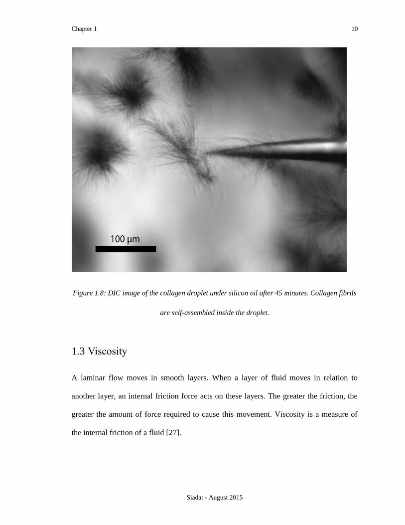
Figure 1.8: DIC image of the collagen droplet under silicon oil after 45 minutes. Collagen fibrils
are self-assembled inside the droplet.
1.3 Viscosity
A laminar flow moves in smooth layers. When a layer of fluid moves in relation to
another layer, an internal friction force acts on these layers. The greater the friction, the
greater the amount of force required to cause this movement. Viscosity is a measure of
the internal friction of a fluid [27].

Chapter 1 11
Siadat - August 2015
The laminar flow in Plane Couette flow (Figure 1.9) is a simple flow that shows the
concept of viscosity. Couette flow is a fluid between two rigid plates where the lower
plate is fixed and the top plate moves with a constant velocity u0 in its own plane.
Assuming a fixed driving force, the velocity of the moving plate can be determined by
the viscosity of the fluid. The more viscous the fluid the slower the top plate moves.
According to Newton’s law of viscosity for laminar flows,
𝜏 = 𝜂𝑑𝑢
𝑑𝑦 , 𝜏 =
𝐹
𝐴 (1.1)
dynamic or absolute viscosity (η) is defined as the ratio of shear stress (τ) to the velocity
gradient (du/dy) between two plates. Fluids that follow Newton’s law are called
Newtonian fluids [27]. Newtonian fluids like water are homogeneous. In a non-
Newtonian flow, viscosity is dependent on shear stress, shear strain rate, and time. Some
biological samples like whole blood behave as non-Newtonian fluids.
Figure 1.9: Couette flow induced by relative motion of two plates
𝑉𝑒𝑙𝑜𝑐𝑖𝑡𝑦 𝑢0
X direction
Y Direction
U (y)

Chapter 1 12
Siadat - August 2015
The viscosity of a fluid is highly dependent on thermodynamic factors such as
temperature and pressure. Liquid viscosity decreases with temperature:
𝑙𝑛𝜂
𝜂0≈ 𝑎 + 𝑏 (
𝑇0𝑇) + 𝑐 (
𝑇0𝑇)2
(1.2)
where T is absolute temperature, η0 is known viscosity at known temperature T0, and a, b,
and c are constants. On the other hand, gas viscosity increases with temperature:
𝜂
𝜂0≈
{
(
𝑇
𝑇0)𝑛
𝑃𝑜𝑤𝑒𝑟 𝑙𝑎𝑤
(𝑇𝑇0)
32(𝑇0 + 𝑆)
𝑇 + 𝑆 𝑆𝑢𝑡ℎ𝑒𝑟𝑙𝑎𝑛𝑑 𝑙𝑎𝑤
(1.3)
where n and S are constants [28].
1.4 Viscosity Measurement
Measurement of viscosity is essential in many fields therefore several methods and
devises have been developed suitable for specific circumstances and materials. Sample
size, working conditions, time consumption, cost, continuous measurement, and fluid
phase are some of the important factors in selecting the appropriate viscosity
measurement method.
The SI (International System of Units) unit of dynamic viscosity is Pa.s or kg/(s.m) which
sometimes refer to as Poiseuille (symbol PI) Named after the French physician Jean
Louis Marie Poiseuille (1797 - 1869). The CGS (centimetre–gram–second system of
units) unit of dynamic viscosity is poise (symbol P) which is equivalent to 0.1 Pa.s. In

Chapter 1 13
Siadat - August 2015
most everyday applications, centipoise (symbol cP) which is 0.1 Pa.s is used as the
dynamic viscosity unit. Most of fluids have viscosities between 0.5 to 1000 cP [29].
Many viscometers measure kinematic viscosity υ which is define as
𝜐 =𝜂
𝜌 (1.4)
Therefore, the density of fluid must be known to measure the dynamic viscosity. The
CGS unit of kinematic viscosity is square centimetres per second or stokes (symbol St).
One stokes is equal to the dynamic viscosity in poise divided by the density of the fluid in
gram per cubic centimetres [27, 29].
A viscometer is a device used to measure the viscosity of a Newtonian fluid and a
rheometer usually used for fluids with viscosities varying with flow conditions. There are
two basic methods to measure the resistance of a fluid to flow. Either an object moves
through a stationary fluid, or the fluid flows through a stationary object. Here some types
of standard laboratory viscometers and rheometers are introduced.
1.4.1 Capillary Viscometers
The kinematic viscosity of Newtonian fluids can be determined using capillary
viscometers which is one of the earliest widely used methods due to their simple design
and process [29]. They cover the range from 0.2 to 300,000 cSt. Figure 1.10 shows a
schematic of a capillary viscometer. Kinematic viscosity can be determined by measuring
the flow rate of a known volume of a fluid through the capillary tube with a known
diameter and known length. The dynamic viscosity is equal to

Chapter 1 14
Siadat - August 2015
𝜐 =𝜋𝑎4𝛥𝑃
8𝑄(𝐿 + 𝑛𝑎)+
𝑚𝜌𝑄
8𝜋(𝐿 + 𝑛𝑎) (1.5)
where Q is the flow rate, a is the radius of the capillary tube, L is the length of the tube,
∆P is pressure drop along the tube, ρ is the fluid density, n and m are correction factors
[29-31]. The correction factors (viscometer constants) depend on the local gravity, fluid
density, surface tension [32], temperature, fluid volume, expansion coefficient of fluid
and glass [27].
Figure 1.10: Schematic of a capillary viscometer
Viscosity measurement using capillary viscometers is simple and cheap, though it has
some weaknesses. This method is time consuming and requires a large volume of fluid.
P2 P1

Chapter 1 15
Siadat - August 2015
Being limited to the Newtonian fluids is the biggest disadvantage of capillary viscometers
[27].
1.4.2 Falling-Body Viscometer
A falling-body viscometer can be used to measure the fluid viscosity by measuring the
elapsed time of a sphere or cylinder shaped body travelling inside a viscous fluid. The
more viscous the fluid the more time the body takes to travel a fixed distance [27]. A
simple schematic illustration is shown is Figure 1.11.
Figure 1.11: Schematic of a falling-body viscometer design. A spherical body is released and
accelerated to the terminal velocity (VT). The time the sphere takes to travel a length L is
measured.

Chapter 1 16
Siadat - August 2015
Based on Stokes’ law the force that slows down a sphere travelling through a viscous
fluid is related to the fluid viscosity and the velocity and radius of the sphere. This drag
force can be measured by
𝐹𝑑 = 6𝜋𝜂𝑅𝑢 (1.6)
where Fd is the drag force, R is the radius, and u is the velocity of the sphere [27, 33, 34].
The terminal velocity can be measured by the force balance between the Stokes drag
force and the force caused by gravity Fg (Figure 1.12):
𝐹𝑔 =4
3𝜋𝑅3(𝜌𝑝 − 𝜌𝑓)𝑔 (1.7)
Figure 1.12: Falling sphere through a liquid. The drag force, Fd, acts on the opposite direction of
the gravity force, Fg.
Fd
Fg

Chapter 1 17
Siadat - August 2015
where ρp and ρf are respectively the density of sphere and fluid and g is the gravitational
acceleration. Therefore, the resulting terminal velocity is given by
𝑉𝑇 =2
9
(𝜌𝑝 − 𝜌𝑓)
𝜂𝑔𝑅2 (1.8)
In this method, fluid viscosity can be measured only in a laminar and fully developed
flow with small Reynolds number [27].
1.4.3 Rotational Viscometer
Rotational viscometers measure the resistance of a fluid to torque. In these viscometers, a
rotor is immersed in a fluid and is rotated at a constant speed. The fluid viscosity is
proportional to the torque on the surface of viscometer. The working equation that relates
the torque to the viscosity is defined by the viscometer geometry [27, 33].
An example of these viscometers is the concentric cylinder viscometer. This viscometer
is made of two concentric cylinders containing a fluid between them. One or both of the
cylinders rotate (usually one cylinder is stationary and the other rotates with constant
velocity) and the torque on the stationary cylinder is measured. Figure 1.13 represents a
schematic of a concentric cylinder. The fluid viscosity can be calculated by equation
(1.9):
𝜂 = 2𝜋𝑅2𝜏 4𝜋 [(𝛼2𝑅2
𝛼2) (𝜔𝑜 − 𝜔𝑖)]⁄ (1.9)
where R is the radius of the inner cylinder, τ is the shear stress per unit length of the inner
cylinder, α is the ratio of the radius of the outer cylinder to the radius of the inner

Chapter 1 18
Siadat - August 2015
cylinder, ωo and ωi are respectively the angular velocity of the outer and inner cylinders
[35].
Figure 1.13: Schematic of a concentric cylinder viscometer. The inside cylinder rotates at a
constant angular velocity, 𝜔, and the torque, M, of the fluid is measured by a strain gauge on the
fixed cylinder
Another example of rotational viscometer is the cone-plate. In the cone-plate viscometer,
the test fluid is contained in a small gap between a flat cone (with reference angle less
than 3°) and a flat plate. The apex of the cone just touches the plate surface. The cone (or
the plate) rotates in a constant speed and the induced torque on the other surface is
measured. The main advantage of this design is the existence of a constant shear rate at
all locations between the cone and the plate. The reason is that as the distance between

Chapter 1 19
Siadat - August 2015
the cone and the plate increases, the linear velocity also increases. Figure 1.14 shows a
schematic of a cone-plate viscometer.
Figure 1.14: Schematic of a cone-plate viscometer. The fluid viscosity can be calculated by
measuring the applied torque to rotate the cone at a constant velocity.
The fluid viscosity can be calculated by equation (1.10):
𝜂 = 3𝐺𝜓 2𝜋𝑅3𝜔⁄ (1.10)
where G is the torque on the cone, ψ is the cone angle in radians, R is the radius of the
cone base, and ω is the angular velocity [36].
1.4.4 Oscillating-Body Viscometer
Oscillating-body viscometers contains a thermally controlled chamber and a magnetically
influenced piston (or blade). An electromagnetic field causes the piston to move back and
forth inside the chamber. The fluid viscosity can be determined according to Newton’s
Plate
Cone Liquid

Chapter 1 20
Siadat - August 2015
law of viscosity, and the piston oscillation time and distance. Figure 1.15 shows a
schematic of an oscillating-piston viscometer [27].
Figure 1.15: Schematic of an oscillating-piston viscometer. The absolute viscosity is obtained by
measuring the time required for the piston to move the travel distance.
The oscillating piston viscometers are widely used for small sample viscosity
measurement. It can be used with different size of pistons to cover a vast range of
viscosity from 0.1 to 2000 cP.
1.4.5 Vibrating Viscometer
Vibrating viscometers can determine the fluid viscosity by measuring the damping of an
oscillating electromechanical resonator [37]. Oscillating sphere and tuning fork are two
types of vibrating viscometers. The measurement principle of these viscometers is that
Piston
Chamber
Travel Distance
Electromagnets

Chapter 1 21
Siadat - August 2015
the product of the fluid viscosity and density is proportional to the viscous damping of
the oscillation amplitude.
The damping of the resonator can be usually measured by the required power to maintain
the oscillator vibration at constant amplitude. Another method is the measurement of the
decay time. The higher the viscosity, the shorter the decay time [29].
In the oscillating sphere viscometers, a stainless steel sphere oscillates with constant
amplitude and the viscosity is calculated based on the required power to maintain the
oscillation. In the tuning fork viscometers fluid viscosity and density can be measured
separately from the bandwidth and the frequency of the vibrating fork resonance [29].
Figure 1.16 and Figure 1.17 show schematics of these vibrational viscometers [38].
Figure 1.16: Schematic of oscillating sphere viscometer.
Transducer
Flow

Chapter 1 22
Siadat - August 2015
Figure 1.17: Schematic of a tuning fork viscometer
1.5 Surface Viscometry
The interpretation of surface viscometry is complicated due to the unbalance of attracting
forces by the nearby molecules [39]. Contribution of the airflow above the surface and
the three-dimensional solution subphase is not completely determined in the surface drag
forces [40]. The usual method for surface viscometry are based on two broad categories:
torque measurement [41] or particle traction [42].
Petkov et al. [42] measured the viscosity of a monolayer between sodium dodecyl sulfate
and hexadecyltrimethylammonium bromide. They used an external capillary force to
Temperature Sensor
Electromagnetic Unit
Direction of
Vibration
Oscillator
Sample

Chapter 1 23
Siadat - August 2015
move a submillimetre-size sphere. The equation of motion of the sphere was solved and
the viscosity was calculated based on the sphere drag coefficient.
Waugh [43, 44] used a continuum mechanical approach to measure the surface viscosity.
A fluid moved through a vesicle containing 20 - 65 µm tethers and the magnitude of the
force acting on the tether was measured using Stokes drag force. The surface viscosity
was calculated by knowing the rate of tether growth, and the force on the vesicle.
Ziemann et al. [45] used a magnetically driven bead micro-rheometer to measure the
local viscoelastic moduli of entangled actin networks. They used the viscosity of the fluid
and Stokes force to calibrate the driving force. Bausch et al. [46] used this micro-
rheometer to measure the viscoelastic parameters of the surface of adhering fibroblasts.
Particle tracking techniques used to track 4.5 µm paramagnetic microspheres. The
viscosity was determined using the viscoelastic response of the cells. A theory of
diffusion of proteins in a membrane coupled to a solid surface [47] was used to estimate
the viscosity of the cytoplasm.
1.6 Molecular Rotors
Molecular rotors are fluorescent molecules with the capability to go through twisted
intramolecular charge transfer (TICT). The TICT molecules consist of three parts: an
electron donor, an electron acceptor, and an electron-rich spacer unit which brings the
donor and the acceptor units together. The donor and the acceptor units rotate relative to
each other, and consequently the fluorescence emission changes with this rotation [48-
50].

Chapter 1 24
Siadat - August 2015
The emission intensity of the TICT molecules depends on the viscosity and polarity of
their solvent while it has been shown that the emission intensities of molecular rotors are
more sensitive to the solvent viscosity than polarity [51]. Molecular rotors come to be
fluorescent only when their rotation is inhibited and therefore they can be used in
microscopic scale for viscosity measurement of biological samples in vitro and vivo
when the commercial viscosity measurement instruments are not applicable [49, 52-56].
The dynamic viscosity of a solvent is related to its fluorescence quantum yield, Φ, based
on the Forster-Hoffmann equation:
𝑙𝑜𝑔𝜙 = 𝐴 + 𝐵(𝑙𝑜𝑔 𝜂) (1.11)
where A and B are respectively temperature and dye dependent constants [57-59].
Haidekker et al. [60] used fluorescent molecular rotors to measure blood plasma
viscosity. They successfully measured the viscosity of plasma-pentastarch mixtures in a
range of 1 to 5 cP. Kung et al. [55] used Benzylidene malononitriles (DCVJ) a molecular
rotor to investigate the polymerization of tubulin at concentrations less than 2.5 mg/mL.
They showed the molecular rotors bind to tubulin and their quantum yield increases with
increasing tubulin concentration. Haidekker et al. [51] showed the peak emission
intensity of DCVJ depends on the viscosity of solvent. They used mixtures of ethylene
glycol and glycerol as the solvent covering a vast range of viscosity up to 945 cP.
Fluorescence lifetimes of the molecular rotors are viscosity-dependent. Kuimova et al.
[61] used meso-substituted 4,4′-difluoro-4-bora-3a,4adiaza-s-indacene as a molecular
rotor in mixtures of methanol-glycerol and showed the fluorescence lifetime increases
from 0.7 ± 0.05 to 3.8 ± 0.1 ns with increasing the mixture viscosity from 28 to 950 cP.

Chapter 1 25
Siadat - August 2015
Using fluorescence-lifetime imaging microscopy (FLIM), intracellular viscosity can be
calculated by measuring the fluorescent lifetime of the molecular rotors [61-63].
1.7 Summary
Mechanical viscometers are usually time consuming and unable to measure the viscosity
of biological micro-samples. The new and powerful method based on the molecular
rotors is suitable for some biological samples in vivo and in vitro. However, more studies
are necessary to validate this method for other biological samples. In addition, using
molecular rotors requires accessibility to confocal microscopy for FLIM, which is not
practical for our experimental setup.
Brownian motion is a powerful way to measure fluid viscosity. In chapter 2, the
Brownian motion of microspheres in the collagen droplet is investigated and the
restriction of this viscosity measurement method for the fiber pulling experiment is
discussed.
To measure the viscosity of the micro-layer on top of the collagen droplet, an optical
method was used in the exact experimental situation. In chapter 3 and 4, the viscosity and
collagen concentration within the droplet were estimated from the measured velocity of
magnetic microspheres in the solution when the droplet was positioned in the uniform
region of a magnetic field produced by a permanent magnet. Each magnetic microsphere
travels in the direction of magnetic lines with a constant velocity, which is related to the
viscosity based on Stokes Law.

Chapter 2 26
Siadat - August 2015
2 BROWNIAN MOTION OF
MICROSPHERES
2.1 Introduction
Brownian motion is a classical experiment to measure the viscosity of a solution.
Suspended particles in a fluid randomly collide with the atoms or molecules in the fluid.
These collisions are thought to result in a random walk of particles in the fluid, called
Brownian motion. Robert Brown first reported this phenomenon in 1827 [64].
The measure of the speed of diffusion in these random movements is characterized by the
diffusion coefficient (D). The diffusion coefficient can be measured by the mean square
displacement (MSD) of particles and the lag time. For an isotropic and unrestricted
translational diffusion, the mean square displacement of particles can be expressed as
{
⟨(∆𝑟)2⟩ = 2𝐷. ∆𝑡, 𝑜𝑛𝑒 𝑑𝑖𝑚𝑒𝑛𝑠𝑖𝑜𝑛
⟨(∆𝑟)2⟩ = 4𝐷. ∆𝑡, 𝑡𝑤𝑜 𝑑𝑖𝑚𝑒𝑛𝑠𝑖𝑜𝑛
⟨(∆𝑟)2⟩ = 6𝐷. ∆𝑡, 𝑡ℎ𝑟𝑒𝑒 𝑑𝑖𝑚𝑒𝑛𝑠𝑖𝑜𝑛
(2.1)
where ⟨(∆r)^2⟩ is the mean square displacement, and ∆t is the lag time.

Chapter 2 27
Siadat - August 2015
In 1905, Albert Einstein predicted the diffusion coefficient of a spherical particle based
on the physical properties of the medium and particle
𝐷 =𝑘𝐵𝑇
6𝜋𝜂𝑟 (2.2)
where kB is the Boltzmann constant, T the temperature, η the viscosity of the medium,
and r the radius of particle [65].
2.2 Experimental Method
A back of the envelop calculation reveals that the one dimensional mean free path within
100 milliseconds acquisition time for a one micrometre diameter particle in water at room
temperature is about 300 nanometre while this number for a sample fluid with a viscosity
of 1000 cp is less than 10 nanometre. In order to measure these small motions, a Gaussian
can be fitted to the one dimensional displacement histogram. When the mean
displacement is zero, the variance of the Gaussian is equal to the MSD.
𝑉𝑎𝑟 (∆𝑥) = ⟨∆𝑥2⟩ − ⟨∆𝑥⟩2 (2.3)
In our implementation of the experiment, green-fluorescent beads (Flow Cytometry Sub-
micron Particle Size Reference Kit, LifeTechnologies, ranging in diameter from 0.02 µm
to 2.0 µm, Catalog number: F13839) were suspended in water at room temperature. To
simulate the collagen fiber pulling experimental setup, a 125 µl volume of water
containing one-micrometre green fluorescent beads was pipetted on an 8 mm cover glass
placed on the stage of a microscope (Nikon inverted microscope eclipse TE2000-E). The
Brownian motions of the fluorescent beads were recorded by a CoolSNAP HQ2 CCD

Chapter 2 28
Siadat - August 2015
camera and a Nikon Plan Fluor ELWD 20x/0.45 objective (0.32 µm/pix). Images were
taken at the rate of 4.3 frame per seconds for one minute (230 milliseconds acquisition
time).
2.3 Vibrational Noise
ImageJ (FIJI, TrackMate Plugin) software was used to find and track the suspended
microspheres. Figure 2.1 shows a sample of the trajectory of the microspheres. Because
of the fiber pulling experimental setup, the medium is not completely protected from
vibrational noises. So the microspheres do not move in a random walk and as it is
obvious in Figure 2.1, the mean displacement is not zero.
2.4 Reducing Error
To reduce the error of drift and vibrational noises, the average of one-dimensional
movement in X and Y directions were subtracted from the data. A MATLAB code was
used to post process the tracked beads by ImageJ software, obtain the new mean
displacement, and calculate the viscosity of the medium. Figure 2.2 shows the histogram
bar chart and the probability distribution of one-dimensional displacements.
The post processing of data resulted in a viscosity of 1.17 cp for water at room
temperature (n=3). Therefore, the same method was used to measure the viscosity of
collagen droplets with known concentrations and viscosities. Nutragen (Advanced
BioMatrix, Bovine Collagen Solution, Type I, 6 mg/ml, Catalog #5010-50ML) was
diluted using 0.01M hydrochloric acid to obtain collagen concentration of 0 to 6 mg/ml.

Chapter 2 29
Siadat - August 2015
For each concentration, a 125 µl volume of collagen solution was pipetted on an 8 mm
cover glass on the microscope stage.
Figure 2.1: The trajectory of 1 µm beads inside a water droplet at room temperature. Different
beads are shown with different colors. It can be seen that in this experimental setup the drift
forces are dominant and the beads do not experience a random walk.

Chapter 2 30
Siadat - August 2015
Figure 2.2: Histogram bar chart of one-dimensional displacements. The Brownian motion of one-
micrometre beads in water were recorded with 230 ms acquisition time.
2.5 Results
The Brownian motions of one-micrometre fluorescent beads were tracked on the surface
of the droplet for four minutes for each sample. The viscosity of collagen solution
samples were measured using ImageJ software and the MATLAB code as mentioned
before. The calculated viscosities were compared to provided viscosity-concentration
data by Advanced BioMatrix (Figure 2.3).

Chapter 2 31
Siadat - August 2015
Figure 2.3: Viscosity of known concentration collagen solutions. The blue dots are the viscosity-
concentration data provided by Advanced BioMatrix. The red squares are measured viscosities of
known concentration collagen solutions.
In the viscosities higher than approximately 40 cp, the noise in the system is dominant
and the Brownian motion of beads is not detectable. Therefore, this method of subtracting
the drift of beads does not work in collagen droplets with high concentrations.
0
20
40
60
80
100
120
140
160
180
0.0 1.0 2.0 3.0 4.0 5.0 6.0 7.0
Vis
cosi
ty, c
p
Concentration, mg/ml

Chapter 2 32
Siadat - August 2015
2.6 Discussion
The diffusion of particles can be increased by using nanometre sized quantum dots
instead of microspheres. Even though, the noise in the system also increases due to
smaller size particles. In the other hand, using bigger particles can decrease the noise of
drift motions. Nevertheless, they cannot be used to measure the viscosity of the droplet
surface micro-layer.
Using a magnetic field to move particles can be a solution to this problem. A magnetic
field can be applied near the droplet and force some magnetic microspheres to move in
the direction of magnetic field. If the particles are big enough, the Brownian motion of
particles can be ignored in compared to their movement due to magnetic force. The
magnetic field and the viscosity measurement of collagen droplet are described in the
next chapter.

Chapter 3 33
Siadat - August 2015
3 MAGNETIC MICROSPHERES
MOTION DUE TO AN
APPLIED MAGNETIC FIELD
3.1 Force Balance on Magnetic Microspheres
There are two types of forces acting on a magnetic microsphere in a viscous solution and
in the presence of a magnetic field: the magnetic force in the direction of the magnetic
lines and the drag force in the opposite direction (Figure 3.1).

Chapter 3 34
Siadat - August 2015
Figure 3.1: The magnetic and drag forces acting on a magnetic microsphere.
The drag force on the magnetic microsphere can be calculated by Stokes Law:
𝐹𝑑⃗⃗⃗⃗ = −6𝜋𝜂𝑅�⃗� (3.1)
where η is the dynamic viscosity of the solution, R and u are respectively the radius and
velocity of the magnetic microsphere. The most common relationship used to measure
the magnetic force acting on a magnetic particle is
𝐹𝑀⃗⃗⃗⃗ ⃗ =𝑉∆𝑥
𝜇0(�⃗� . 𝛻)�⃗� (3.2)
where V is the particle’s volume, ∆x is the difference in magnetic susceptibility between
the particle and the solution, μ0 is the permeability of the vacuum which is equal to
𝜇0 = 4𝜋 ∗ 10−7, 𝑇𝑚𝐴−1 (3.3)
and B is the applied magnetic field [54].
Permanent Magnet
Cover
Collagen Droplet
Magnetic
Force Drag
Force

Chapter 3 35
Siadat - August 2015
The collagen droplet was placed close to the magnet and exactly on the centerline of its
surface, which has a uniform magnetic field. Neglecting gravitational and conventional
forces, the force balance for the magnetic microsphere is defined by
∑𝐹 = 𝐹𝑀⃗⃗⃗⃗ ⃗ + 𝐹𝑑⃗⃗⃗⃗ = 𝑚𝑎 (3.4)
where m is the magnetic microsphere mass and vector a is its acceleration.
3.2 Magnetic Field Measurement
The magnetic field was supplied by a permanent magnet (BY0Y08-N52, K&J Magnetics,
Inc.) and its strength and gradient were respectively measured as 593*10-4 T, and 2.9
T/m by a gauss meter at a distance of 53 mm from the center of the magnet (Figure 3.2).
3.3 Terminal Velocity
Considering the force balance on the magnetic microspheres in the direction of magnetic
field lines and neglecting the change of magnetic force throughout the droplet, magnetic
microspheres reach to a terminal velocity toward the center of the magnet. Since the
experiment happens in a short time, the accuracy of the viscosity measurement depends
on the time that takes particles to reach this terminal velocity.
Numerical methods were used to estimate the time before all the particles reach to the
constant terminal velocity. Microspheres velocity at each time point (ui) can be predicted
based on the initial velocity and the rate of change of velocity:

Chapter 3 36
Siadat - August 2015
Figure 3.2: Variation of the magnetic field with distance from the magnet. The slope of the line
fitted on the data point at 53 mm distance is 29 gauss/mm or 2.9 T/m.
𝑢𝑖 = 𝑢𝑖−1 +𝑑𝑢
𝑑𝑡|𝑖−1
𝛥𝑡 (3.5)
Also according to the equation (3.4), the rate of change of velocity can be written as:
𝑑𝑢
𝑑𝑡|𝑖= 𝑎𝑖 =
𝐹𝑚 − 𝛼𝑢𝑖𝑚
(3.6)
where constant α is equal to
𝛼 = 6𝜋𝜂𝑅 (3.7)
The terminal velocity was calculated using MATLAB (The MATLAB code is available
in appendix). The initial velocity was assumed equal to zero. The diameter, magnetic
-1400
-1200
-1000
-800
-600
-400
-200
0
30 40 50 60 70 80
Ma
gn
etic
Fie
ld, g
au
ss
Distance from the Magnet, mm

Chapter 3 37
Siadat - August 2015
susceptibility, and density of the magnetic microsphere where respectively presumed as
2.8 µm, 0.5, and 1600 kg/m3 based on the common magnetic microspheres in the market.
The results are shown in Figure 3.3 for a sample solution with the viscosity of 100 cp (~5
mg/mL collagen) and in Figure 3.4 for ~98% glycerol by volume at 20°C with a viscosity
of 1000 cp. Time steps of 0.1 ns were used in this numerical method. The Runge-Kutta
method was also used to solve the equation (3.5) and the result was the same.
Figure 3.3: Terminal velocity of the microspheres in a solution with the viscosity of 100 cp.
Figure 3.3 and Figure 3.4 demonstrate that the magnetic microspheres reach to their
terminal velocity in a few nanoseconds in our experimental situation. Therefore the
microspheres velocity throughout the experiment can be considered constant and the
equation (3.4) written as
0
50
100
150
200
250
300
350
0 10 20 30 40 50 60
Vel
oci
ty, n
m/s
Time, ns

Chapter 3 38
Siadat - August 2015
Figure 3.4: Terminal velocity of the microspheres in a solution with the viscosity of 1000 cp.
∑𝐹 = 𝐹𝑀⃗⃗⃗⃗ ⃗ + 𝐹𝑑⃗⃗⃗⃗ = 0 (3.8)
So the terminal velocity can be calculated by setting the magnitudes of the magnetic and
the drag forces equal to each other. Equation (3.9) shows the final form of the terminal
velocity,
𝑣 =2
9
𝑅2𝜒
𝜂𝜇0(𝐵𝑥
𝜕𝐵𝑥𝜕𝑥
) (3.9)
where the x-direction is in the same direction as magnetic force and χ is the initial
magnetic susceptibility of the particles (the magnetic susceptibility of the medium is
neglected).
0
5
10
15
20
25
30
35
0 1 2 3 4 5 6 7
Vel
oci
ty, n
m/s
Time, ns

Chapter 3 39
Siadat - August 2015
The resulting velocity for the microspheres from equation (3.9) is 303 nm/s in a solution
with the viscosity of 100 cp and 30 nm/s in a solution with the viscosity of 1000 cp,
which is compatible with the results from the numerical methods. Therefore, in a
potential concentrated droplet surface with a viscosity of 1000 cp, the magnetic
microspheres with the assumed properties and specified magnetic field, travel 1800 nm
per each minute. This travel distance is detectable with a Nikon Plan Fluor ELWD
20x/0.45 objective (0.32 µm/pixel).
3.4 Magnetic Susceptibility
In order to calculate the viscosity of the collagen droplet, the equation (3.9) can be
written in the form of
𝜂 =2
9
𝑅2𝜒
𝑣𝜇0(𝐵𝑥
𝜕𝐵𝑥𝜕𝑥
) (3.10)
In this equation, the terminal velocity can be measured experimentally by tracking the
magnetic microspheres in the collagen droplet. In addition, the magnitude and gradient of
the magnetic field can be measured by a gauss meter as described in section 3.2.
However, the magnetic susceptibility of particles usually alternate between lots.
The magnetic susceptibility is the measure of magnetization of a material inside a
magnetic field. The bigger the susceptibility the faster the magnetic microspheres move.
Therefore to precisely measure the magnetic susceptibility of the particles, a
superconducting quantum interference device (SQUID) was used at room temperature,
300 K, to generate the magnetic response of Dynabeads M-270 Carboxylic Acid, Catalog

Chapter 3 40
Siadat - August 2015
number 14305D. These magnetic microspheres have a uniform diameter of 2.8 µm,
density of 1.6 g/cm3, and initial concentration of 2*109 beads/ml (~30 mg/ml). The
magnetization curve is shown in Figure 3.5.
Figure 3.5: Magnetic response of Dynabeads M-270 in a field ranging from - 5 to 5 Tesla.
Oersted (Oe) is the unit of magnetic field (H) in CGS system of units and is equal to 103/4π A/m.
emu/g is the unit of mass magnetization which is equal to A.m2/kg.
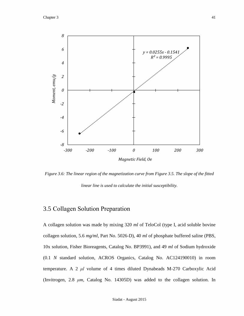
The susceptibility of the magnetic microspheres, χ = 0.512, is measured from the slope of
the line fitted to the initial part of the magnetization curve (weak fields). The slope of the
line is multiplied by 4π*ρ to dimensionless the magnetic susceptibility Figure 3.6.
-15
-10
-5
0
5
10
15
-60000 -40000 -20000 0 20000 40000 60000
Mo
men
t, e
mu
/g
Magnetic Field, Oe
Chapter 3 41
Siadat - August 2015
Figure 3.6: The linear region of the magnetization curve from Figure 3.5. The slope of the fitted
linear line is used to calculate the initial susceptibility.
3.5 Collagen Solution Preparation
A collagen solution was made by mixing 320 ml of TeloCol (type I, acid soluble bovine
collagen solution, 5.6 mg/ml, Part No. 5026-D), 40 ml of phosphate buffered saline (PBS,
10x solution, Fisher Bioreagents, Catalog No. BP3991), and 49 ml of Sodium hydroxide
(0.1 N standard solution, ACROS Organics, Catalog No. AC124190010) in room
temperature. A 2 μl volume of 4 times diluted Dynabeads M-270 Carboxylic Acid
(Invitrogen, 2.8 μm, Catalog No. 14305D) was added to the collagen solution. In
y = 0.0255x - 0.1541R² = 0.9995
-8
-6
-4
-2
0
2
4
6
8
-300 -200 -100 0 100 200 300
Mo
men
t, e
mu
/g
Magnetic Field, Oe

Chapter 3 42
Siadat - August 2015
addition, non-magnetic microspheres were also added to remove the motion of magnetic
microspheres caused by other forces acting on the microspheres in the droplet. The non-
magnetic microspheres were introduced to the solution by adding 2 μl of 1 part Fluoro-
Max green fluorescent polymer microspheres (Thermo Scientific, 1.9 μm, Catalog No.
G0200) to 9 part deionized water to the solution.
A 125 µl volume of the well-mixed collagen solution was transferred on an 8 mm circular
cover glass. The droplet was surrounded by an aluminium cylinder. Using this aluminium
cylinder and a dual valve pressure controller (Alicat Scientific), the humidity of the
chamber decreased to approximately zero percent. The pressure controller was set up on
0.022 psig. In order to not disturb the air inside the cylinder, the collagen droplet was
pipetted on the cover glass through a hole on the cylinder.
In the similar experimental condition as the fiber pulling experiment but with the
presence of the magnetic bar, DIC images of the surface of the droplet were captured at a
rate of 1 frame per second for 30 seconds after 0, 1, 2, and 3 minutes of nitrogen gas
flowing over the droplet. The nitrogen gas was stopped after the mentioned times and
DIC images were taken using a Nikon inverted microscope eclipse TE2000-E with a
CoolSNAP HQ2 CCD camera and a Nikon Plan Fluor ELWD 20x/0.45 objective (0.32
µm/pix). With the purpose of determining the thickness of the viscous layer on the
droplet’s surface, the same experiment was done in 20, 40, 60, and 1000 μm below the
droplet’s surface after 150 seconds of nitrogen gas flowing over the droplet. The
experimental setup is shown in Figure 3.7 and Figure 3.8.

Chapter 3 43
Siadat - August 2015
Figure 3.7: The experimental setup. The inverted microscope, the zero humidity chamber, and the
pressure controller are shown in the image.
The Zero Humidity Chamber
The Pressure Controller

Chapter 3 44
Siadat - August 2015
Figure 3.8: The zero humidity chamber on the microscope stage.
y = 0.0255x - 0.1541R² = 0.9995
-8
-6
-4
-2
0
2
4
6
8
-300 -200 -100 0 100 200 300
Mo
men
t, e
mu
/g
Magnetic Field, Oe
The collagen droplet
Cylinder holes for pipetting
the collagen droplet
The permanent Magnet

Chapter 4 45
Siadat - August 2015
4 IMAGE ANALYSIS AND
RESULTS
The Magnetic and non-magnetic microspheres were distinguished based on their size and
tracked using MATLAB. A MATLAB code was adapted from a method of digital video
microscopy by Crocker and Grier [66] and Gao and Kilfoil [67]. The code finds and
tracks microspheres and produces the trajectory of each microsphere as its output. The
features are identified by finding high intensity regions in each frame. Then the magnetic
and non-magnetic microspheres are recognized based on their shape, size, and intensity.
A feature can be reidentified when it disappears for a few frames.
4.1 Grouped Microspheres
During the experiment, some of the close by magnetic microspheres were aggregated and
form long chains. The corresponding magnetic and drag forces for these grouped
microspheres are different from the single ones. Therefore, a minimum distance of three
micrometre between identified features was set to exclude all of the grouped

Chapter 4 46
Siadat - August 2015
microspheres. An example of the aggregated microspheres in glycerol 50% is shown in
Figure 4.1.
Figure 4.1: Single and grouped microspheres in the presence of the magnetic field.
4.2 Local Forces on the Magnetic Microspheres
In addition to magnetic and drag forces explained in section 3.1, there are other local
forces acting on the magnetic microspheres. For instance, the evaporation of the droplet,
the flow of nitrogen gas, and surface tensions can complicate the understanding of force
balance on each microsphere. Therefore, non-magnetic microspheres were introduced to
the collagen solution to overcome this problem and measure the movement of magnetic
microspheres only due to the magnetic field.

Chapter 4 47
Siadat - August 2015
The non-magnetic microspheres were recognized by their size (1.9 µm). For each frame,
the velocity of individual magnetic microspheres were subtracted by the velocity of the
closest (maximum distance of 100 μm) non-magnetic microspheres. Then, the average of
the relative velocities in the direction of the magnetic field for all magnetic microspheres
was used to calculate the viscosity of the surface of the droplet (equation (3.10)).
Figure 4.2 shows the inverted DIC image of the magnetic and non-magnetic
microspheres inside the collagen droplet after 150 seconds.
Figure 4.2: The 2.8 µm magnetic (M) and 1.9 µm non-magnetic (N) microspheres are
distinguished by their size.
The trajectories of magnetic and non-magnetic microspheres at 1000 µm depth, 20 µm
depth, and on the droplet surface are shown respectively in Figure 4.3, Figure 4.4, and
Chapter 4 48
Siadat - August 2015
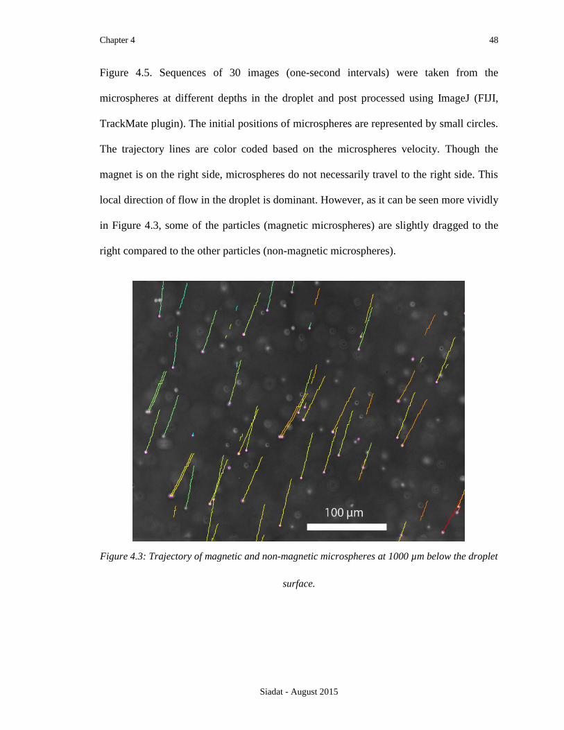
Figure 4.5. Sequences of 30 images (one-second intervals) were taken from the
microspheres at different depths in the droplet and post processed using ImageJ (FIJI,
TrackMate plugin). The initial positions of microspheres are represented by small circles.
The trajectory lines are color coded based on the microspheres velocity. Though the
magnet is on the right side, microspheres do not necessarily travel to the right side. This
local direction of flow in the droplet is dominant. However, as it can be seen more vividly
in Figure 4.3, some of the particles (magnetic microspheres) are slightly dragged to the
right compared to the other particles (non-magnetic microspheres).
Figure 4.3: Trajectory of magnetic and non-magnetic microspheres at 1000 µm below the droplet
surface.

Chapter 4 49
Siadat - August 2015
Figure 4.4: Trajectory of magnetic and non-magnetic microspheres at 20 µm below the droplet
surface.
Figure 4.5: Trajectory of magnetic and non-magnetic microspheres on the droplet surface.

Chapter 4 50
Siadat - August 2015
4.3 Collagen Viscosity
The collagen concentration was predicted based on data provided by Advanced
BioMatrix, Inc. for viscosity and concentration of PureCol (bovine collagen solution,
type I) in the range of 0.88 to 6 mg/mL (Figure 4.6).
Figure 4.6: Viscosity of collagen for concentrations less than 6 mg/ml. The polynomial trend line
fitted on the data is used to predict the viscosity of higher concentrations.
4.4 Concentration of the Droplet Surface
The change of surface concentration was measured over the first three minutes after the
droplet was placed on the cover glass and exposed to the nitrogen gas. Figure 4.7 shows a
y = 0.4988x3 + 1.451x2 + 1.1647x + 0.0256
R² = 0.9995
0
20
40
60
80
100
120
140
160
180
0 1 2 3 4 5 6 7
Vis
cosi
ty, cp
Collagen Concentration, mg/ml

Chapter 4 51
Siadat - August 2015
linear increase of the surface concentration during the fiber pulling experiment. The data
demonstrates a concentration of approximately 14 mg/mL collagen after 150 seconds on
the droplet surface.
Figure 4.7: Concentration of the droplet surface over three minutes (n=5 per time point).
4.5 Thickness of the Dense Layer
Figure 4.8 shows the drastic change of concentration in a micro-layer on the droplet
surface. The concentration decreased to 7.9 mg/ml at only 20 µm below the surface. This
shows the thickness of the thin layer of dense collagen is less than 20 µm and the fiber
can only initiate in this region. The data also shows the concentration of bulk region does
0
5
10
15
20
25
0 50 100 150 200 250
Conce
ntr
ati
on, m
g/m
L
Time, sec

Chapter 4 52
Siadat - August 2015
not change markedly. The initial solution was made at 4.4 mg/ml and it increased to 4.6
after 150 seconds inside the droplet (1000 µm below the surface).
Figure 4.8: Concentration of the droplet after 150 seconds at 0, 20, 40, 60, and 1000 µm below
the surface (n=5 per data point)
4.6 Confirming Fiber Pull Time
Existence of the permanent magnet in the experiment chamber effects on the nitrogen gas
flow. Furthermore, the presence of magnetic microspheres might change the collagen
behavior in the droplet. Validation of the fiber pulling experiment in the new setup of
experiment was investigated by repeating the fiber pulling experiment. The fiber was
0
2
4
6
8
10
12
14
16
18
20
1 10 100 1,000
Conce
ntr
ati
on, m
g/m
L
Depth, µm

Chapter 4 53
Siadat - August 2015
pulled after the same wait time (150 seconds) and with same maximum pull speed (240
µm/s).
The pulled fibers were immersed in a dish of PBS. The DIC images of these fibers were
similar to the previous fibers. The organized structure of these fibers are shown in and
Figure 4.9. Comparing these images to Figure 1.7 which was pulled under silicon oil can
illustrate the organization of collagen fibrils in these fibers.
Figure 4.9: DIC image of collagen fiber in PBS. The collagen fiber was pulled after 150 seconds
in the new experimental setup for viscosity measurement.

Chapter 4 54
Siadat - August 2015
4.7 Control Test
The post processing method and experimental setup of viscosity measurement was
controlled by measuring the viscosity of glycerol 99% v/v. The glycerol 99% v/v was
made by adding a 4 μl volume of the magnetic microspheres (Dynabeads M-270
Carboxylic Acid, Invitrogen, 2.8 μm, Catalog No. 14305D, 1 part to 3 part deionized
water) and a 4 μl of non-magnetic microspheres (Fluoro-Max green fluorescent polymer
microspheres, Thermo Scientific, 1.9 μm, Catalog No. G0200, 1 part to 9 part deionized
water) to a 1040 ml volume of glycerol (Fisher Scientific, 99.8% assay, f.w. 92.09, CAS
56-81-5).
Viscosity of the bulk region of the droplet was measured with the same method that used
for collagen droplet. An average viscosity of 1120 cp was measured for glycerol 99% v/v
at 21°C temperature (n = 9, standard deviation = 121). The viscosity of glycerol 99% v/v
at 21°C temperature is reported as 1086 cp [68]. The approximation error of 3.13% shows
the high accuracy of the experiment.
4.8 Summary
In the present study, the viscosity of a collagen droplet was measured as a function of
time and depth. In the experimental setup, a magnetic field was set up near the collagen
droplet and the movements of some magnetic microspheres were tracked inside the
droplet. Then the viscosity of the droplet was measured using the Stokes drag force on
each magnetic microshere.

Chapter 4 55
Siadat - August 2015
The concentration of collagen was estimated based on the viscosity-concentration data
for the collagen source. The post processing of data showed a concentration of
approximately 14 mg/ml was attained at the top surface of the droplet after 150 seconds.
The thickness of this layer was measured less than 20 µm. The concentration dropped to
8 mg/ml when it measured at 20 µm below the surface.
The suspended particles on the top of the droplet may possibly experience a complicated
movement. For instance, surface tensions and airflow over the droplet can change the
force balance on the microspheres. In addition, the diameter and magnetic susceptibility
of the microspheres are not completely constant. These uncertainties are the most
important source of error in this viscosity measurement method.
The result of this study gave an important information in the critical surface
concentration where collagen fibers can be formed, which can lead to the design of a
more efficient and predictable methodology to produce highly organized collagen fibers.

Chapter 5 56
Siadat - August 2015
5 APPENDICES
APPENDIX 1: BROWNIAN MOTION OF THE MICROSPHERES ................................................ 57
APPENDIX 2: TERMINAL VELOCITY OF THE MICROSPHERES IN A SOLUTION WITH A
VISCOSITY OF 100 CP ................................................................................................. 64
APPENDIX 3: DETERMINING THE TERMINAL VELOCITY OF THE MICROSPHERES USING
RUNGE-KUTTA 4TH ORDER METHOD ......................................................................... 66
APPENDIX 4: RENAMING AND INVERTING OF FRAMES ....................................................... 68
APPENDIX 5: VELOCITY OF THE MAGNETIC MICROSPHERES .............................................. 69
APPENDIX 6: VELOCITY OF THE NON-MAGNETIC MICROSPHERES ...................................... 71
APPENDIX 7: VISCOSITY MEASUREMENT ........................................................................... 73

Chapter 5 57
Siadat - August 2015
APPENDIX 1: BROWNIAN MOTION OF THE MICROSPHERES
1. clear
2. clc
3. close all
4. % The image sequences of the beads on the surface of the collagen droplet was
post processed using ImageJ and FIJI
5. % Threshold = 22
6. % Linking Max Distance = 50 pix
7. % Closing Max Distance = 50 pix
8. % Gap-Closing Max Frame = 10
9. % The result of the beads tracking was extracted to an Excel file, “AllFrames”,
and imported into Matlab as “RawData”
10. filename = 'AllFrames.xlsx';
11. sheet = 1;
12. RawData = xlsread(filename);
13. % Column 1: Bead ID
14. % Column 2: Bead X Position
15. % Column 3: Bead Y Position
16. % Column 4: Frame Number
17. % 20X Objective (0.33 micrometer per pixle)
18. RawData(:,2) = 0.33.*RawData(:,2);
19. RawData(:,3) = 0.33.*RawData(:,3);
20. BeadID = RawData(:,1);
21. % The first column of RawData is Beads ID numbers
22. x = RawData(:,2);
23. % The second column of RawData is the X position of beads in micrometer

Chapter 5 58
Siadat - August 2015
24. y = RawData(:,3);
25. % The third column of RawData is the Y position of beads in micrometer
26. Frame = RawData(:,4);
27. % The fourth column of RawData is the frame number of beads
28. f = max(Frame);
29. [H,~] = size(RawData);
30. % The (delta x / delta frame) of each bead was calculated for all frames
31. for i=1:H-1
32. if BeadID(i) == BeadID(i+1)
33. RawData(i+1,5) = (x(i+1)-x(i))/(Frame(i+1)-Frame(i));
34. RawData(i+1,6) = (y(i+1)-y(i))/(Frame(i+1)-Frame(i));
35. else
36. RawData(i+1,5) = NaN;
37. RawData(i+1,6) = NaN;
38. end
39. end
40. for i=1:H
41. if RawData(i,5) == 0
42. RawData(i,5) = NaN;
43. end
44. if RawData(i,6) == 0
45. RawData(i,6) = NaN;
46. end
47. end
48. % Delta X and Delta Y movement of beads were classified according to the frame
number
49. FrameDataX = NaN;
50. FrameDataY = NaN;

Chapter 5 59
Siadat - August 2015
51. for i=1:f
52. k = 1;
53. for j=1:H
54. if Frame(j) == i
55. FrameDataX(i,k) = RawData(j,5);
56. FrameDataY(i,k) = RawData(j,6);
57. k = k+1;
58. end
59. end
60. end
61. [~,L] = size(FrameDataX);
62. for i=1:f
63. for j=1:L
64. if FrameDataX(i,j) == 0
65. FrameDataX(i,j) = NaN;
66. end
67. if FrameDataY(i,j) == 0
68. FrameDataY(i,j) = NaN;
69. end
70. end
71. end
72. % Average of Delta X and Delta Y movement of beads
73. FrameDataXMean = NaN(f,1);
74. FrameDataYMean = NaN(f,1);
75. for i=1:f
76. FrameDataXMean(i,1) = nanmean(FrameDataX(i,:));
77. FrameDataYMean(i,1) = nanmean(FrameDataY(i,:));
78. end

Chapter 5 60
Siadat - August 2015
79. % To reduce the error of drift or vibrational noise, the average of delta X and Y
were subtracted from original delta X and Y
80. FrameDeltaX = NaN;
81. FrameDeltaY = NaN;
82. for i=1:f
83. for j=1:L
84. if isreal(FrameDataX(i,j))
85. FrameDeltaX(i,j) = FrameDataX(i,j)-FrameDataXMean(i,1);
86. end
87. if isreal(FrameDataY(i,j))
88. FrameDeltaY(i,j) = FrameDataY(i,j)-FrameDataYMean(i,1);
89. end
90. end
91. end
92. for i=1:f
93. for j=1:L
94. if FrameDeltaX(i,j) == 0
95. FrameDeltaX(i,j) = NaN;
96. end
97. if FrameDeltaY(i,j) == 0
98. FrameDeltaY(i,j) = NaN;
99. end
100. end
101. end
102. SumFrameDeltaX = NaN(f,1);
103. SumFrameDeltaY = NaN(f,1);
104. for i=1:f
105. if isnan(FrameDeltaX(i,1))
106. SumFrameDeltaX(i,1) = NaN;

Chapter 5 61
Siadat - August 2015
107. SumFrameDeltaY(i,1) = NaN;
108. else
109. SumFrameDeltaX(i,1) = nansum(FrameDeltaX(i,:));
110. SumFrameDeltaY(i,1) = nansum(FrameDeltaY(i,:));
111. end
112. end
113. % The data have a zero mean displacement
114. figure(1)
115. subplot(2,1,1)
116. nbins = 200;
117. hist(SumFrameDeltaX,nbins);
118. hold on;
119. subplot(2,1,2)
120. hist(SumFrameDeltaY,nbins);
121. hold on;
122. % Seperation of all delta x and y data for each n frame
123. [H,L] = size(FrameDeltaX);
124. X = NaN;
125. k = 1;
126. for i=1:H
127. for j=1:L
128. if isfinite(FrameDeltaX(i,j))
129. X(k,1) = FrameDeltaX(i,j);
130. k = k+1;
131. end
132. end
133. end
134. [H,L] = size(X);

Chapter 5 62
Siadat - August 2015
135. for i=1:H
136. for j=1:L
137. if X(i,j) == 0
138. X(i,j) = NaN;
139. end
140. end
141. end
142. pd = NaN;
143. SD = NaN;
144. MSDX = NaN;
145. D = NaN;
146. Vis = NaN;
147. for i=1:L
148. figure(i+1)
149. nbins = 100;
150. hist(X(:,i),nbins);
151. % Creates a histogram bar chart of one-dimensional displacements (delta x) for
every 10 frames(4.35 fps)
152. pd = fitdist(X(:,i),'normal');
153. % Fit probability distribution object to the histogram bar
154. SD = pd.sigma;
155. % Standard Deviation
156. k = -2:0.01:2;
157. PDF = pdf(pd,k);
158. % Probability density function of the probability distribution object
159. PDF = PDF ./ max(PDF);
160. % Normalised
161. % scale to y axis
162. y=ylim;
163. PDF = PDF*y(2);
164. hold on;

Chapter 5 63
Siadat - August 2015
165. plot(k,PDF,'r-','LineWidth',2);
166. MSDX(i) = SD.^2;
167. % The variance of the Gaussian fit (pd) is equivalent to the one-dimensional
Mean Square Displacement if the mean displacement is zero [um/frame]
168. t = 233.493*10^-3;
169. % The time between data points [s]
170. D(i) = MSDX(i)./(2*t);
171. % Diffusion [um^2/s]
172. a = (1/2)*(10^-6);
173. % Bead radius
174. Vis(i) = (1000)*(1.3806488*(10^-23))*(294)/(6)/(3.14)/a./(D(i).*(10^-12));
175. % Viscosity [cp]
176. end
177. figure(L+2)
178. T = 5:10:10*L-5;
179. plot(T,Vis,'b.');
180. xlabel('Time [s]');
181. ylabel('Viscosity [cp]');

Chapter 5 64
Siadat - August 2015
APPENDIX 2: TERMINAL VELOCITY OF THE MICROSPHERES
IN A SOLUTION WITH A VISCOSITY OF 100 CP
1. clc; 2. clear all; 3. h = 0.1e-9; 4. % Time steps [s] 5. t = 0:h:5e-8; 6. % Time [s] 7. v = zeros(1,length(t)); 8. % Velocity of Microspheres [m/s] 9. v(1) = 0; 10. % Initial velocity 11. n = 100e-3; 12. % Viscosity [kg/(s.m)] 13. R = (2.8e-6)/2; 14. % Radius of Microspheres [m] 15. rho = 1.6e3; 16. % Density of Microspheres [kg/m^3] 17. V = 4/3*pi*R^3; 18. % Volume of Microspheres [m^3] 19. C2 = 6*pi*n*R/rho/V; 20. s = 0.5; 21. % Susceptibility of the Microspheres 22. B = 593e-4; 23. % Magnetic Field [T] 24. dB = 2.953; 25. % Magnetic Field's Gradient [T/m] 26. mu = 4*pi*10^-7; 27. % The Permeability of the vacuum [T.m/A] 28. C1 = s/rho/mu*B*dB;

Chapter 5 65
Siadat - August 2015
29. for i=2:(length(t)-1) 30. v(i) = v(i-1)+(C1-C2*v(i-1))*h; 31. end
32. filename = '100cp.xlsx'; 33. xlswrite(filename,t,'Time'); 34. xlswrite(filename,v,'Velocity');

Chapter 5 66
Siadat - August 2015
APPENDIX 3: DETERMINING THE TERMINAL VELOCITY OF
THE MICROSPHERES USING RUNGE-KUTTA 4TH ORDER
METHOD
1. clc; 2. clear all; 3. h = 0.1e-9; 4. % step size 5. x = 0:h:5e-8; 6. y = zeros(1,length(x)); 7. y(1) = 0; 8. % initial condition 9. n = 100e-3; 10. % Viscosity [cp] 11. R = (2.8e-6)/2; 12. % Magnetic Bead's Radius [m] 13. rho = 1.6e3; 14. % Magnetic Bead's Density [kg/m^3] 15. V = 4/3*pi*R^3; 16. % Magnetic Bead's Volume [m^3] 17. C2 = 6*pi*n*R/rho/V; 18. % Constant Number 19. s = 0.5; 20. % Bead's magnetic susceptibility 21. B = 593e-4; 22. % Magnetic Field [T] 23. dB = 2.953; 24. % Magnetic Field's Gradient [T/m] 25. mu = 4*pi*10^-7; 26. % The permeability of the vacuum [T.m/A] 27. C1 = s/rho/mu*B*dB; 28. % Constant Number 29. F_xy = @(t,r) C1-C2*r;

Chapter 5 67
Siadat - August 2015
30. for i=1:(length(x)-1) 31. % calculation loop 32. k_1 = F_xy(x(i),y(i)); 33. k_2 = F_xy(x(i)+0.5*h,y(i)+0.5*h*k_1); 34. k_3 = F_xy((x(i)+0.5*h),(y(i)+0.5*h*k_2)); 35. k_4 = F_xy((x(i)+h),(y(i)+k_3*h)); 36. y(i+1) = y(i) + (1/6)*(k_1+2*k_2+2*k_3+k_4)*h; 37. % main equation 38. end
39. y' 40. figure(1) 41. plot(x*1e9,y*1e9) 42. title('Prediction of Terminal Velocity by Runge-Kutta 4th Order Method') 43. xlabel('Time [ns]') 44. ylabel('Velocity of Magnet Beads [nm/s]')

Chapter 5 68
Siadat - August 2015
APPENDIX 4: RENAMING AND INVERTING OF FRAMES
1. % Renaming a File in the Current Folder 2. a ='E:\Experiments\...\'; 3. A = dir( fullfile(a, '*.tif') ); 4. fileNames = { A.name }ν; 5. for iFile = 1 : numel( A ) 6. newName = fullfile(a, sprintf( 'fov1_%04d.tif', iFile ) ); 7. movefile( fullfile(a, fileNames{ iFile }), newName ); 8. end
9. % Inverting all the frames
10. clear 11. clc 12. close all 13. fovn = 1;
14. % ID# for the series of images (typically, one field of view) 15. pathin = ' E:\Experiments\...\'; 16. numframes = xlsread('Book1.xlsx','Experiment Data');
17. % The number of images you have in your series 18. for x = 1:numframes 19. strnam=[pathin 'fov' num2str(fovn) '\fov' num2str(fovn) '_' num2str(x,'%04i')
'.tif']; 20. img = imread(strnam); 21. img = abs(4096-img); 22. imwrite(img, strnam); 23. end

Chapter 5 69
Siadat - August 2015
APPENDIX 5: VELOCITY OF THE MAGNETIC MICROSPHERES
1. clear 2. clc 3. close all 4. load res_fovM; 5. A(:,1) = res(:,8); 6. A(:,2) = res(:,1); 7. A(:,3) = res(:,2); 8. A(:,4) = res(:,6); 9. % Column 1: Bead ID 10. % Column 2: Bead X Position 11. % Column 3: Bead Y Position 12. % Column 4: Frame Number
13. T = xlsread('Book1.xlsx','Recorded Data', 'B:B'); % The time at which the image
was recorded (Sorted by frame#) 14. % 20X Objective (0.32 micrometer per pixle) 15. A(:,2) = 0.32.*A(:,2); 16. A(:,3) = 0.32.*A(:,3); 17. [n,~] = size(A); 18. A(:,5) = NaN; 19. A(:,6) = NaN; 20. % The velocity of each bead was calculated for all frames
21. for i=1:n-1 22. if A(i,1) == A(i+1,1) && A(i+1,4)-A(i,4)==1 23. A(i+1,5) = (A(i+1,2)-A(i,2))./(T(A(i+1,4))-T(A(i,4))); 24. A(i+1,6) = (A(i+1,3)-A(i,3))./(T(A(i+1,4))-T(A(i,4))); 25. else 26. A(i+1,5) = NaN; 27. A(i+1,6) = NaN; 28. end

Chapter 5 70
Siadat - August 2015
29. end 30. save Magnet.mat A;

Chapter 5 71
Siadat - August 2015
APPENDIX 6: VELOCITY OF THE NON-MAGNETIC
MICROSPHERES
1. clear 2. clc 3. close all
4. load res_fovF; 5. B(:,1) = res(:,8); 6. B(:,2) = res(:,1); 7. B(:,3) = res(:,2); 8. B(:,4) = res(:,6); 9. % Column 1: Bead ID 10. % Column 2: Bead X Position 11. % Column 3: Bead Y Position 12. % Column 4: Frame Number
13. T = xlsread('Book1.xlsx','Recorded Data', 'B:B');
14. % The time at which the image was recorded (Sorted by frame#) 15. % 20X Objective (0.32 micrometer per pixle) 16. B(:,2) = 0.32.*B(:,2); 17. B(:,3) = 0.32.*B(:,3);
18. [n,~] = size(B); 19. B(:,5) = NaN; 20. B(:,6) = NaN;
21. % The velocity of each bead was calculated for all frames 22. for i=1:n-1 23. if B(i,1) == B(i+1,1) && B(i+1,4)-B(i,4)==1 24. B(i+1,5) = (B(i+1,2)-B(i,2))./(T(B(i+1,4))-T(B(i,4)));

Chapter 5 72
Siadat - August 2015
25. B(i+1,6) = (B(i+1,3)-B(i,3))./(T(B(i+1,4))-T(B(i,4))); 26. else 27. B(i+1,5) = NaN; 28. B(i+1,6) = NaN; 29. end 30. end
31. save Fluor.mat B;

Chapter 5 73
Siadat - August 2015
APPENDIX 7: VISCOSITY MEASUREMENT
1. clear
2. clc
3. close all
4. load Fluor;
5. load Magnet;
6. [n,~] = size(A);
7. [m,~] = size(B);
8. C = NaN(n,4);
9. T = xlsread('Book1.xlsx','Recorded Data', 'B:B');
10. % The time at which the image was recorded (Sorted by frame#)
11. for i=1:n
12. for j=1:m
13. L = sqrt((A(i,2)-B(j,2))^2 + (A(i,3)-B(j,3))^2);
14. if B(j,4)==A(i,4) && L < 3
15. A(i,5)=NaN;
16. A(i,6)=NaN;
17. end
18. end
19. end
20. for i=1:n-1
21. for j=i+1:n
22. L = sqrt((A(i,2)-A(j,2))^2 + (A(i,3)-A(j,3))^2);
23. if A(j,4)==A(i,4) && L < 3
24. A(i,5)=NaN;
25. A(i,6)=NaN;
26. end
27. end
28. end

Chapter 5 74
Siadat - August 2015
29. for i=1:n
30. C(i,1) = A(i,4);
31. C(i,2) = T(A(i,4));
32. L = 100;
33. for j=1:m
34. if B(j,4)==A(i,4)
35. LL = sqrt((A(i,2)-B(j,2))^2 + (A(i,3)-B(j,3))^2);
36. if LL < L
37. L = LL;
38. C(i,3) = A(i,5)-B(j,5);
39. C(i,4) = A(i,6)-B(j,6);
40. end
41. end
42. end
43. end
44. % Measure the velosity in X & Y direction for each bead [um/s]
45. Vx = nanmean(C(:,3));
46. Vy = nanmean(C(:,4));
47. D(:,1) = C(:,1);
48. D(:,2) = C(:,2);
49. Alpha = 0.05;
50. rep = 1;
51. [D(:,3), IDX, OUTLIERSX] = deleteoutliers(C(:,3),Alpha,rep);
52. [D(:,4), IDY, OUTLIERSY] = deleteoutliers(C(:,4),Alpha,rep);
53. Vx_Grubbs = nanmean(D(:,3));
54. Vy_Grubbs = nanmean(D(:,4));
55. STx = nanstd(D(:,3));
56. STy = nanstd(D(:,4));
57. Z = [Vx,Vy;Vx_Grubbs,Vy_Grubbs;STx,STy];
58. Res = 'Result.xlsx';
59. xlswrite(Res,Z,'B2:C4')

Chapter 5 75
Siadat - August 2015
60. R = (2.8/2)*10^-6; % Magnetic Bead's Radius [m]
61. m = 4*pi*10^-7; % The Permibility of the vacuum [T.m/A]
62. x = 0.51; % Bead's magnetic susceptibility
63. b = 593e-4; % Magnetic Field [T]
64. dB = 2.953; % Magnetic Field's Gradient [T/m]
65. vis = 1000*(2/9/(Vx_Grubbs*10^-6)*R^2*x/m*b*dB); % Bead's Velocity cp]
66. xlswrite(Res,vis,'B5:B5')

Chapter 6 76
Siadat - August 2015
6 REFERENCES
1. Kadler, K.E., et al., Collagen fibril formation. Biochem J, 1996. 316 ( Pt 1): p. 1-
11.
2. Canty, E.G. and K.E. Kadler, Procollagen trafficking, processing and
fibrillogenesis. J Cell Sci, 2005. 118(Pt 7): p. 1341-53.
3. Kadler, K.E., et al., Collagens at a glance. Journal of Cell Science, 2007.
120(12): p. 1955-1958.
4. Friess, W., Collagen--biomaterial for drug delivery. Eur J Pharm Biopharm,
1998. 45(2): p. 113-36.
5. Kadler, K.E., A. Hill, and E.G. Canty-Laird, Collagen fibrillogenesis: fibronectin,
integrins, and minor collagens as organizers and nucleators. Curr Opin Cell Biol,
2008. 20(5): p. 495-501.
6. Grinnell, F., Fibroblast biology in three-dimensional collagen matrices. Trends
Cell Biol, 2003. 13(5): p. 264-9.
7. Kannus, P., Structure of the tendon connective tissue. Scand J Med Sci Sports,
2000. 10(6): p. 312-20.
8. Birk, D.E. and R.L. Trelstad, Extracellular compartments in tendon
morphogenesis: collagen fibril, bundle, and macroaggregate formation. J Cell
Biol, 1986. 103(1): p. 231-40.
9. Birk, D.E., et al., Collagen fibril bundles: a branching assembly unit in tendon
morphogenesis. Development, 1989. 107(3): p. 437-43.
10. Birk, D.E., M.V. Nurminskaya, and E.I. Zycband, Collagen fibrillogenesis in situ:
fibril segments undergo post-depositional modifications resulting in linear and
lateral growth during matrix development. Dev Dyn, 1995. 202(3): p. 229-43.
11. Birk, D.E., et al., Collagen fibrillogenesis in situ: fibril segments become long
fibrils as the developing tendon matures. Dev Dyn, 1997. 208(3): p. 291-8.
12. Kadler, K.E., Y. Hojima, and D.J. Prockop, Assembly of collagen fibrils de novo
by cleavage of the type I pC-collagen with procollagen C-proteinase. Assay of
critical concentration demonstrates that collagen self-assembly is a classical
example of an entropy-driven process. J Biol Chem, 1987. 262(32): p. 15696-701.

Chapter 6 77
Siadat - August 2015
13. Nurminskaya, M.V. and D.E. Birk, Differential expression of genes associated
with collagen fibril growth in the chicken tendon: identification of structural and
regulatory genes by subtractive hybridization. Arch Biochem Biophys, 1998.
350(1): p. 1-9.
14. Kadler, K.E., Y. Hojima, and D.J. Prockop, Collagen fibrils in vitro grow from
pointed tips in the C- to N-terminal direction. Biochem J, 1990. 268(2): p. 339-43.
15. Fratzl, P., Collagen : structure and mechanics. 2008, New York: Springer. xviii,
506 p.
16. van der Rest, M. and R. Garrone, Collagen family of proteins. FASEB J, 1991.
5(13): p. 2814-23.
17. Boot-Handford, R.P. and D.S. Tuckwell, Fibrillar collagen: the key to vertebrate
evolution? A tale of molecular incest. Bioessays, 2003. 25(2): p. 142-51.
18. Hendershot, L.M. and N.J. Bulleid, Protein-specific chaperones: the role of hsp47
begins to gel. Curr Biol, 2000. 10(24): p. R912-5.
19. Porter, S., et al., The ADAMTS metalloproteinases. Biochem J, 2005. 386(Pt 1):
p. 15-27.
20. Risteli, J., et al., Radioimmunoassay for the Pyridinoline Cross-Linked Carboxy-
Terminal Telopeptide of Type-I Collagen - a New Serum Marker of Bone-
Collagen Degradation. Clinical Chemistry, 1993. 39(4): p. 635-640.
21. Akeson, W.H., et al., Collagen cross-linking alterations in joint contractures:
changes in the reducible cross-links in periarticular connective tissue collagen
after nine weeks of immobilization. Connect Tissue Res, 1977. 5(1): p. 15-9.
22. Eyre, D.R., M.A. Paz, and P.M. Gallop, Cross-linking in collagen and elastin.
Annu Rev Biochem, 1984. 53: p. 717-48.
23. Reiser, K., R.J. McCormick, and R.B. Rucker, Enzymatic and nonenzymatic cross-
linking of collagen and elastin. FASEB J, 1992. 6(7): p. 2439-49.
24. Kadler, K., Matrix loading: assembly of extracellular matrix collagen fibrils
during embryogenesis. Birth Defects Res C Embryo Today, 2004. 72(1): p. 1-11.
25. Hulmes, D.J.S., Building collagen molecules, fibrils, and suprafibrillar structures.
Journal of Structural Biology, 2002. 137(1-2): p. 2-10.
26. Paten, J., Investigation into the mechano-chemistry of de novo collagen assembly.
2014.
27. Gupta, S.V., Viscometry for liquids : calibration of viscometers. Cham : Springer,
2014. Vol. Springer series in materials science ; v.194. 2014.
28. White, F.M., Fluid mechanics. 6th ed. McGraw-Hill series in mechanical
engineering. 2008, New York: McGraw-Hill. xiii, 864 p. ill.
29. Viswanath, D.S., Viscosity of liquids : theory, estimation, experiment, and data.
2007, Dordrecht: Springer. xiii, 660 p.
30. Daniels, F., Experimental physical chemistry. 5th ed. 1956, New York,: McGraw-
Hill. 482 p.
31. Bingham, E.C., Fluidity and plasticity. 1st ed. 1922, New York etc.: McGraw-Hill
book company, inc. xi, 440 p.
32. Barr, G., Errors in viscometry due to surface tension. National Physical
Laboratory, Teddington, 1946.
33. Dinsdale, A. and F. Moore, Viscosity and its measurement. Monographs for
students. 1962, London,

Chapter 6 78
Siadat - August 2015
New York,: Published on behalf of the Institute of Physics and the Physical Society by
Chapman and Hall;
Reinhold. 67 p.
34. Wakeham, W.A., et al., Measurement of the transport properties of fluids.
Experimental thermodynamics. 1991, Oxford England ; Boston
Boca Raton, Fla.: Blackwell Scientific Publications ;
Distributed in the USA and North America by CRC Press. xx, 459 p.
35. Dontula, P., C.W. Macosko, and L.E. Scriven, Origins of concentric cylinders
viscometry. Journal of Rheology, 2005. 49(4): p. 807-818.
36. McKennell, R., Cone-Plate Viscometer. Analytical Chemistry, 1956. 28(11): p.
1710-1714.
37. Yabuno, H., et al., Self-excited vibrational viscometer for high-viscosity sensing.
Journal of Applied Physics, 2014. 116(12).
38. Akpek, A., C. Youn, and T. Kagawa, Temperature Measurement Control Problem
of Vibrational Viscometers Considering Heat Generation and Heat Transfer
Effect of Oscillators. 2013 9th Asian Control Conference (Ascc), 2013.
39. Osborne, M.F.M., The theory of the measurement of surface viscosity. Kolloid-
Zeitschrift und Zeitschrift für Polymere, 1968. 224(2): p. 150-161.
40. Alonso, C. and J.A. Zasadzinski, Linear dependence of surface drag on surface
viscosity. Physical Review E, 2004. 69(2).
41. Ghaskadvi, R.S., et al., Shear response of Langmuir monolayers of heneicosanoic
(C-21) acid studied using a torsion pendulum. Physical Review E, 1996. 54(2): p.
1770-1773.
42. Petkov, J.T., et al., Precise method for measuring the shear surface viscosity of
surfactant monolayers. Langmuir, 1996. 12(11): p. 2650-2653.
43. Waugh, R.E., Surface Viscosity Measurements from Large Bilayer Vesicle Tether
Formation .1. Analysis. Biophysical Journal, 1982. 38(1): p. 19-27.
44. Waugh, R.E., Surface Viscosity Measurements from Large Bilayer Vesicle Tether
Formation .2. Experiments. Biophysical Journal, 1982. 38(1): p. 29-37.
45. Ziemann, F., J. Radler, and E. Sackmann, Local Measurements of Viscoelastic
Moduli of Entangled Actin Networks Using an Oscillating Magnetic Bead Micro-
Rheometer. Biophysical Journal, 1994. 66(6): p. 2210-2216.
46. Bausch, A.R., et al., Local measurements of viscoelastic parameters of adherent
cell surfaces by magnetic bead microrheometry. Biophysical Journal, 1998.
75(4): p. 2038-2049.
47. Evans, E. and E. Sackmann, Translational and Rotational Drag Coefficients for a
Disk Moving in a Liquid Membrane-Associated with a Rigid Substrate. Journal of
Fluid Mechanics, 1988. 194: p. 553-561.
48. Rotkiewicz, K., K.H. Grellmann, and Z.R. Grabowski, Reinterpretation of the
anomalous fluorescense of p-n,n-dimethylamino-benzonitrile. Chemical Physics
Letters, 1973. 19(3): p. 315-318.
49. Haidekker, M.A. and E.A. Theodorakis, Environment-sensitive behavior of
fluorescent molecular rotors. J Biol Eng, 2010. 4: p. 11.

Chapter 6 79
Siadat - August 2015
50. Goh, W.L., et al., Molecular rotors as conditionally fluorescent labels for rapid
detection of biomolecular interactions. J Am Chem Soc, 2014. 136(17): p. 6159-
62.
51. Haidekker, M.A., et al., Effects of solvent polarity and solvent viscosity on the
fluorescent properties of molecular rotors and related probes. Bioorg Chem,
2005. 33(6): p. 415-25.
52. Gavvala, K., et al., Modulation of excimer formation of 9-(dicyano-
vinyl)julolidine by the macrocyclic hosts. Phys Chem Chem Phys, 2013. 15(1): p.
330-40.
53. Iwaki, T., et al., Antibodies for fluorescent molecular rotors. Biochemistry, 1993.
32(29): p. 7589-92.
54. Sawada, S., et al., Fluorescent rotors and their applications to the study of G-F
transformation of actin. Anal Biochem, 1992. 204(1): p. 110-7.
55. Kung, C.E. and J.K. Reed, Fluorescent molecular rotors: a new class of probes
for tubulin structure and assembly. Biochemistry, 1989. 28(16): p. 6678-86.
56. Vaccaro, G., et al., Direct monitoring of self-assembly of copolymeric micelles by
a luminescent molecular rotor. Chem Commun (Camb), 2013. 49(76): p. 8474-6.
57. Förster, T.H., G., Effect of viscosity on the fluorescence quantum yield of some
dye systems.
. Zeitschrift für Physikalische Chemie, 1971. 75: p. 63–76.
58. Kung, C.E. and J.K. Reed, Microviscosity Measurements of Phospholipid-
Bilayers Using Fluorescent Dyes That Undergo Torsional Relaxation.
Biochemistry, 1986. 25(20): p. 6114-6121.
59. Howell, S., et al., Intrinsic and extrinsic temperature-dependency of viscosity-
sensitive fluorescent molecular rotors. J Fluoresc, 2012. 22(1): p. 457-65.
60. Haidekker, M.A., et al., A novel approach to blood plasma viscosity measurement
using fluorescent molecular rotors. Am J Physiol Heart Circ Physiol, 2002.
282(5): p. H1609-14.
61. Kuimova, M.K., et al., Molecular rotor measures viscosity of live cells via
fluorescence lifetime imaging. J Am Chem Soc, 2008. 130(21): p. 6672-3.
62. Levitt, J.A., et al., Membrane-Bound Molecular Rotors Measure Viscosity in Live
Cells via Fluorescence Lifetime Imaging. Journal of Physical Chemistry C, 2009.
113(27): p. 11634-11642.
63. Hungerford, G., et al., Monitoring sol-to-gel transitions via fluorescence lifetime
determination using viscosity sensitive fluorescent probes. J Phys Chem B, 2009.
113(35): p. 12067-74.
64. Brown, R., A brief account of microscopical observations made in the months of
June, July and August, 1827, on the particles contained in the pollen of plants;
and on the general existence of active molecules in organic and inorganic bodies.
1828. p. 161-173.
65. Einstein, A., Über die von der molekularkinetischen Theorie der Wärme
geforderte Bewegung von in ruhenden Flüssigkeiten suspendierten Teilchen.
Annalen der Physik, 1905. 322(8): p. 549-560.
66. Crocker, J.C. and D.G. Grier, Methods of digital video microscopy for colloidal
studies. Journal of Colloid and Interface Science, 1996. 179(1): p. 298-310.

Chapter 6 80
Siadat - August 2015
67. Gao, Y.X. and M.L. Kilfoil, Accurate detection and complete tracking of large
populations of features in three dimensions. Optics Express, 2009. 17(6): p. 4685-
4704.
68. Cheng, N.S., Formula for the viscosity of a glycerol-water mixture. Industrial &
Engineering Chemistry Research, 2008. 47(9): p. 3285-3288.