drsomesh k mathur - apeaweb.org · drsomesh k mathur, phd (corresponding author) associate...
TRANSCRIPT

1
Does GDP and GDP Growth Rates affect Energy Consumption: A Panel Study of Some Developed, Developing and Transition Economies
By
DrSomesh K Mathur, PhD (Corresponding Author)
Associate Professor of Economics,
M: 09935754731. Email: [email protected]
&
Dr.SohiniSahu (Second Author) Assistant Professor of Economics
Email: [email protected]
and
Ishita Ghoshal SSE,Pune
&
Kanak Aggarwal
HSS,IITK
Abstract The present study is an attempt to test the relationship between energyconsumption, energy
efficiency, CO2 Emissions and economic growth for aset of some developed, transition and
developing counties. For thispurpose, panel data on various factors of GDP growth has been
taken for 18developing, 16 transition and 18 developed countries from 1980-2013.The paper
uses the variant of Solow model to provide the economic justification behind the econometric
estimation of regression model whichincludes energy consumption per capita, CO2 emissions
and energyefficiency as one of the independent variables affecting GDP growth of acountry,
among others.To estimate the regression model, the study uses various panel dataestimation

2
methodologies such as: panel data cointegration, panelcausality (assuming homogeneous and
heterogeneous panels), panel VECM,panel VAR and panel data ARDL and SURE. The results
help us to find out he short run and long-run relationship between the policy variables.The paper
also tests the direction of causality between energy consumptionand GDP and per capita GDP
growth by working on the following hypotheses:(a) Neutrality Hypothesis, which holds that there
is no causality (neither direction) between these two variables; (b) Energy
conservationhypothesis, which holds that there is evidence of unidirectional causalityfrom GDP
growth to energy consumption; (c)Growth hypothesis, energy consumption drives GDP growth;
and (d) Feedback hypothesis, which suggestsa bidirectional causal relationship between energy
consumption and GDPgrowth.S-shaped relationship between energy consumption and per capita
GDP isalso tested by hypothesizing that with high GDP, first energyconsumption increases at an
increasing rate and then increases at adecreasing rate.The overall conclusion emerges from the
analysis is that per capita energy consumption has a negative impact on growth of per capita
GDP in developing countries and transition economies but positive impact in case of developed
countries. This may be due to the fact that in developed nations, the energy consumption
expenditures may be more devoted to technological progress in alternative source of oil like
shell gas or in expenditures related to renewable energy intensive technological products. The
developing and transition countries although trying to put efforts in increasing expenditures in
alternative energy sources like non-renewable, oil consumption still seem to not have many
alternatives sources of energy. Therefore, reducing oil expenditures tend to promote growth
among developing countries. Growth, Energy Conservation and Feedback hypotheses tend to
work for developed, transition and developing countries. Also, the direction of causality may run
from growth per capita to energy consumption depicting aS-shaped relation signifying that as
society matures energy consumption increases but at a decreasing rate.
Keywords: Energy Consumption, Economic Growth, Panel Data, Solow Model.
JEL Classification Codes: O13, O47, C33
1. Introduction
Energy is the engine that drives the economy of any nation. In the absence of reliable
energy supply, efforts at socio-economic and technological development cannot yield any
3
positive result. It is essential to the production of all goods and services and hence vital to the
industrial development of any nation. Energy plays an essential role in an economy on both
demand and supply sides. On the demand side, in the form of electricity, itis one of the products
which consumer decides to buy to maximize his/her utility. On the supply side, energy is a key
factor of production in addition to capital, labor and materials. Being a key factor, it plays a vital
role in increasing country’s economic growth and living standards through industrial and
economic development. However, energy consumption and growth per capita do have an impact
on carbon emissions and possibly is responsible for higher carbon emissions and climate change.
Our paper goes on to understand the two way relationship between energy consumption and
growth per capita, FDI/GDP, Trade/GDP and CO2 emissions, among other variables for set of
developed, developing and transition economies.
There exist various studies that examined the relationship between economic growth and
energy consumption. The results of the studies provide mixed conclusions about the direction of
causality between energy consumption and economic growth. In the earlier studies, Kraft and
Kraft (1978) using the time-series data from 1947-1974 for the USA study the causal relationship
between gross energy consumption and GNP. They found the uni-directional relationship
flowing from GNP to energy. This study was followed by many other studies such as Akarca and
Long II (1980), Abosedra and Baghestani (1991), Masih and Masih (1997) and Soytas and Sari
(2003). These studies employ data for single country/countries and find varied results. In
addition to these, Chiang (2005) uses panel data for developing countries and finds short-run and
long-run uni-directional causality flowing from energy to GDP. His result suggests that energy
conservation may harm economic growth in the short-run and in the long run. However, there
also exist some studies which support bi-directional causality between energy consumption and
GDP growth. Those studies are: Glasure (2002), Erdalet al. (2008), Belloumi (2009) among
others. Further, Squalli (2007), Ozturk (2010) and Magazzino (2011) in their studies club all
directions of causality between energy consumption and economic growth into the following
four categories which can be used as research hypotheses in the research focused on studying the
relationship between these two variables. Those hypotheses are:
• Neutrality Hypothesis: which holds that there is no causality (in either direction)
between these two variables;

4
• Energy Conservation Hypothesis: which holds that there is evidence of unidirectional
causality from GDP growth to energy consumption;
• Growth Hypothesis: which assumes energy consumption drives GDP growth; and
• Feedback Hypothesis: which suggests a bidirectional causal relationship between energy
consumption and GDP growth
Howland, Derek Murrow, Lisa Petraglia and Tyler Comings (2009)show that when energy
efficiency is implemented only at individual state level, it has comparatively weaker impact than
when implemented over all states simultaneously. This happens because efficient use of energy
leads to energy savings, increasing comparative national competitiveness, boosting GDPs and
real household income. Increased spending on efficiency measures and decreased spending on
energy go hand in hand. They also show that energy savings leads to lower energy costs which
takes the economy to a more competitive state leading to a higher per capita GDP growth rate.
A report prepared by the Climate Institute on Energy efficiency and economic growth
(2013) considers energy as a factor of production and shows that given higher real energy prices,
efficiency in use of energy contributes positively to economic growth. They go on to show that
empirical evidence on whether energy consumption leads to growth is mixed (mainly due to
model specification and country). They show that energy productivity has increased over time
(GDP per unit of energy used) and efficient use of energy leads to greater economic growth by
reducing energy requirement per unit of output - hence demand and prices fall - competitive cost
advantage appears in trading scenario. The authors go on to estimate energy efficiency and
define energy productivity being determined by energy efficiency, prices and social and sectoral
factors. The analysis of relation between energy efficiency and growth shows a positive relation.
NarendraNathDalei (2016) establishes a non-linear sigmoid relation between energy
consumption and GDP. The study shows that initially energy consumption increases at an
increasing rate with rise in GDP and after a point in time, it increases at a decreasing rate with
further rise in GDP. The study suggests use of alternative or renewable sources of energy instead
of conventional sources is the main reason for this turn of relation. Taking the clue from the
above study , we also test for S-shaped relationship between energy consumption per capita and
growth per capita GDP, FDI/GDP,Trade/GDP and CO2 emissions. Theempirics of S-shaped
relationship below indicate that as society matures, energy consumption increases at a decreasing
rate across the sample.

5
The authors try to understand the relationship between energy consumption and growth
of an economy, among other growth factors, including CO2 emissions, under the framework of a
growth model. If energy consumption and efficiency of energy consumption may be considered
as proxies for the level of technology used for production, then an econometric analysis may be
conducted based on the model specified by Solow for capturing growth of an economy and
variables affecting it. By testing the model for developed, developing and transition countries,
we may be able to pin down the differences with respect to the growth model relations for the
two sets of economies considered. Such a study may be able to bring to limelight how energy
consumption may promote (or not) GDP growth depending on which phase of development the
economy is enjoying during the time period considered. The economy’s phase of development
would prompt different policy implications. Also, the relationship may work from growth per
capita GDP to energy consumption per capita, in particular, mimicking the S-shape relationship,
signifying that as growth increases, energy consumption increases at an increasing rate and then
after the inflection point has been attained, energy consumption increases at a decreasing rate.
The same relationship is tested in the paper for set of developing, developed and transition
economy. Further, the S-shaped relationship is also tested between energy consumption per
capita with CO2 emissions, FDI/GDP and Trade/GDP variables.
For this purpose, the study is divided into five sections including the present introductory
one. Section 2 presents the objectives and rationale of the study. Section 3 provides the
derivation of the economic model which is used as the base for defining the regression equation
for empirical results, the sources of database and methodology used for the empirical analysis in
detail. It also explains the steps of estimation using panel data analysis. In Section 4, empirical
results pertaining to the estimation of regression models have been presented and discussed.
Section 5 concludes the whole study and provides some noteworthy policy implications obtained
from the results.
2. Objectives and Rationale of the study 2.1Objectives
On the basis of mixed results obtained in the literature, the present study tries to evaluate the
relationship between country’s energy consumption and its economic growth by taking the
sample of 18 developed,18 developing countries and 16 transition economies (see appendix
Table A1 for country names). The main objective of the study is to confirm one of the

6
hypotheses given in the previous section mentioning the direction of relationship between energy
consumption and economic growth. The study also evaluates the type of relationship between
these two variables by specifying an economic model behind this, including other variables
affecting economic growth of a country and energy consumption per capita. The study also tests
for the S-shape relationship running from growth per capita to energy consumption per capita.
The study has utilized panel data estimation approach to evaluate the short run and long run
relationships.
2.2 Rationale A glance through the literature reveals various studies related to the topic at hand
throwing light on various aspects. However, a study of comparative analysis among developing,
transition and developed countries over a time period of thirty three years (1980-2013) has not
been attempted. The authors are curious to understand not only the relationship among the
variables mentioned earlier, but also to examine whether the three groups of countries display
similar behavior or not. The authors believe that this analysis and its peculiar results would help
in carving out more efficient policies for developed, transition and developing nations.
3. Empirical Model, Database and Methodology 3.1 Empirical Model
The study follows the variant of the Solow model with technical progress given in
Mankiwet al. (1992) and Jones (2002). With labor augmenting technological progress (A), the
Cobb-Douglas production function becomes:
( )1 0 1 ...(1)t t t tY K AL αα α−= < <
Where Y is level of output; K is capital; and L is labor which is assumed to grow exogenously at
rate n which is equal to:
LnL
=
0
nt
tL L e =
At grows endogenously at rate g and presented as follows: 5 6 74 ...(1.1)gt
t oA A e T H I Eβ β ββ=
The level of technology in (1.1) above is explained by trade openness (T), human capital (H),
share of industry in GDP of the country (I) and expenditure on energy consumption or energy
7
efficiency (E)1. Further, capital grows at K sY Kδ= − . Assuming that a proportion of income is
saved and invested (s) and the level of output per unit of effective labor and stock of capital per
unit of effective labor as YyAL
= and KkAL
= respectively, then the dynamic equation for k is
given as:
( )t tk sy n g kδ= − + +
( )t tk sk n g kα δ = − + +
Where δ is the constant rate of depreciation and it is evident that k converges to its steady state
value ( )0k = .
11
* skn g
α
δ
− = + +
The steady state output per effective labor is:
1* sy
n g s
αα−
= + +
The steady state output per laboris:
1* ...(2)t
sy An g
αα
δ
− = + +
The formulation in (2) can explain why steady state per capita income levels differ among
countries. They differ because countries have different savings rate, technology levels and rate of
growth of population among others.
3.1.1Dynamism around the Steady State It is possible to utilize a more general framework that examines the predictions of the Solow
model for behavior of per capita income out of steady state. Such a framework allows estimation
of the effect of various explanatory variables on per-capita growth rates as well as the speed at
1 The trade openness and human capital are known to be major vehicles for international knowledge and technology spillovers; technology plays a major role in increasing productivity and growth in the industrial sector; whereas, energy consumption expenditure is linked with increase in investments in technological advances in energy resources and more advancement also lead to invent energy efficient resources.

8
which actual income per capita reaches the steady state level of income per-capita. Assuming
other terms zero, the expansion of log y around log y * using Taylor’s expansion provides: *
*
*log loge
y yy yy−= +
*log **
y yyye y−+
=
**
*
y yy ye
y
− =
Similarly, *
*
*
k kkk e
k
− =
Also, the rate of growth of income per effective labor is α times the rate of growth of capital per effective labor.
y ky k
α•
=
y K L Ay K L A
α
= − −
( )t
t
yy s n gy k
α δ
= − + +
***
***
. ( ).
y yy
tk k
k
e yy s n gy e k
α δ−
−
= − + +
In steady state: * *( )sy n g kδ= + +
So *
*
**
( ) ( )y y
y
k kk
y n g e n gy e
δα δ−
−
+ + = − + +
**
**
( ) 1y y
y
k kk
y en gy e
α δ−
−
= + + −

9
* ** *
**
( )y y k k
y k
k kk
y e en gy e
α δ− −
−
− = + +
Asper the Taylors expansion:
log loge
m nm nn−= +
m nn
men
−
≈
logm n mn n−
Using the above, we get
* *
*
( )
y ky y kn gy k
k
α δ
− = + +
* *( ) log /y y kn g
y y kα δ
= + +
{ }* *( ) log log log logy n g y y k ky
α δ = + + − − +
By using * *log log log logy k and y kα α= =
[ ]*(1 )( ) log logy n g y yy
α δ= − + + −
[ ]*log log ...(3)y y yy
λ = −
Where (1 )( )n gλ α δ= − + + is the speed of convergence.Barro and Martin (1995) defined speed
of convergence as rate at which the level of income per effective worker approaches its steady
state which is given as:
(log )
ydy
d yλ
− =

10
The speed of convergence coefficient (λ) is the proportionate change in growth rate caused by
change in initial income per effective labor. Equation (3) shows that growth rate of income per
effective labor is equal to the speed of convergence multiplied by the gap between steady state
and actual level of incomes. Higher the gap, higher would be the growth rates. If the
countries/regions have the same steady state growth and level of incomes, country/regions which
are far away from its steady state will grow at faster rate and catch up with the relatively rich
partner (absolute convergence).Solving the differential equation (3) we get
( ) *
0log log 1 logt t
ty y e e yλ λ− −= + −
Where 0log y is log of initial level of income per effective labor.
( ) ( ) *
0 0log log 1 log 1 logt t
ty y e y e yλ λ− − − = − − + −
To find growth of income per capital we substitute the value of log At which is equal to:
0 4 5 6 7log log log log logA gt T H I Eβ β β β+ + + + + +
and
YyAL
=
yyA
=
We get
( )( )*
0 0log log 1 log logt
ty y e y yλ−− = − −
( )0 0log log 1 log ...(4)t
t iy y e y cλ− − = − − +
Where
( ) [ ]*
4 5 6 71 log log log log logt t
ic e y e gt T H I Eλ λ β β β β− −= − + + + + +
In Equation (4) average per capita growth is found by dividing by time period t on both sides.
Non-linear least squares can be used to estimate equation (4) using cross sectional data. It is to be
noted that if we assume that all economies here have the same steady state level of per capita
income, which in turn implying same structural parameters of the economy, and steady state
growth, then Constantcibecomes c. Further, equation (4) would then imply absolute convergence,
if the coefficient 0(1 ) log 0te of y isλ β−− = > (implying negative relationship between average
growth rate and initial level of GDP per capita).However, the diversities among the economies

11
are quite apparent,conditional convergence is the likely proposition. For conditional
convergence, we can derive growth rate of per capital income after substituting values of steady
state income from (2). Therefore, we get:
( ) ( )
( )
( )
0 0
4
5 6 7 0
log log 1 log 1 log1
1 log( ) log1
+ log log log 1 log
t t
t
t
t
y y e y e s
e n g gt T
H I E e A
λ λ
λ
λ
αα
α δ βα
β β β
− −
−
−
− = − − + −−
− − + + + +−
+ + + −
For cross-sectional study average growth can be found by dividing by time period t
( ) ( )
( )
00
4
5 6 7
1 1log log log log1
1 log( ) log
1 + log log log ... (5)
t t
t
t
e ey y D y st t t
en g g T
tH I E
λ λ
λ
αα
α δ βα
β β β ε
− −
−
− −− = − +−
−′− + + + +
−′ ′ ′+ + +
Where 0log A D= + ε where D is a constant and ε is the country specific shift or shock term.
Time component captures the rate of growth of technology in a panel setup. If the coefficient of
log y0 is > 0 we have conditional beta convergence.However, for empirical analysis, the
following linear equation is estimated using country-wise data over the years. As per the nature
of the data, the study has used the panel data estimation technique to estimate the following
model to show the impact of energy consumption on economic growth.
1 2 3 4 5
6 7 8 9
10
log( ) log( ) log( ) log( ) log( ) log( ) log( ) log( ) log( ) log(
PCGr PC Ratio Gr Ratio
it i it it it it
Ratio PC Ratio
it it it it
Y a b Intial b Savings b Pop b Trade b LifeExpb Industry b Energy b FDI b COb
= + + + + ++ + + ++ ) ... (6)PC
it it itCO Energy ε× +
1 2 3 4 5
6 7 8
9
log( ) log( ) log( ) log( ) log( ) log( ) log( ) log( ) log( )
PCGr PC Ratio Gr Ratio
it i it it it it
Ratio Energy Ratio
it it it
it
Y a b Intial b Savings b Pop b Trade b LifeExpb Industry b Efficiency b FDIb CO
= + + + + ++ + ++ 10 log( ) ... (6.1)PC
it it itb CO Energy ε+ × +
Where PCGr
itY is annual growth rate of GDP per capita; log( )PC
iIntial is the log of initial level of
GDP per capita; log( )Ratio
itSavings is log of ratio of gross domestic savings to GDP; log( )Gr
itPop is
the log ofthe growth rate of population growth (n) +rate of growth of technology(g)which is
assumed to be constant at 3 percent +rate of depreciation(δ) assumed to be constant at 2 percent;
log( )Ratio
itTrade log of the trade to GDP ratio as a proxy for trade openness; log( )itLifeExp is the
log of life expectancy at birth, a proxy for healthy labor force; log( )Ratio
itIndustry is the log of share

12
of industry value added in GDP; log( )PC
itEnergy is the log of energy consumption per capita;
log( )Energy
itEfficiency is the log of efficiency scores plus one of electricity producing energy
industry by using various renewable and non-renewable resources; and log( )Ratio
itFDI is the log of
share of net FDI inflows in GDP2. We have added CO2 emissions and an interactive term of CO2
emissions and energy consumption per capita(both in log form) in (6) and (6.1) hypothesizing
that CO2 emissions entails use of sophisticated technology to develop renewable, which in turn
increases growth per capita. The interactive term is also hypothesized to have a positive impact
on growth per capita.
3.2 Database
To estimate the regression model given in equation (6), panel data of 18 developed, 16
transition and 18 developing countries on the required variables has been used over the period
1980-2013. Country-wise data on all variables has been culled from World Development
Indicators (WDI) provided by the World Bank.Data on all the variables of the regressions are
easily available in the WDI database except the efficiency scores of energy industry. The
efficiency scores of energy industry is calculated using input-oriented technical efficiency3with
constant returns to scale assumption. Year-wise technical efficiency scores of 18 developed and
18 developing countries have been calculated by using three outputs and one input. Due to the
restriction of data availability, the study has taken one input of energy use per capita and three
outputs as electricity production from nuclear sources, renewable sources, excluding
hydroelectric and electricity production from oil, gas and coal sources. The data on all three
outputs is in percentage terms of total electricity production and data on input is at kilogram of
oil equivalent provided by WDI.
3.3 Methodology
As per the nature of the data, the study has used the panel data estimation methodology to
find the relationship between energy consumption and economic growth. Following sub-sections
2 In the study, two different models have been estimated: One with energy consumption per capita (Model given in equation 6) and other with energy efficiency (Model given in equation 6.1) as a one of the independent variable in place of each other. The study has also included share of FDI in GDP as one of the independent variable which is not present in the equation (5) as derived from the economic model. The last four factors in both of the models determine the level of technology in the model. 3 See Cooper et al. (2007).

13
show the panel data estimation methodology utilized to answer the research questions defined in
section 1.
3.3.1 Panel Data Unit-Root Tests for Two Variable Analysis
The study has employed panel data unit root tests to check whether the variables are stationary or
not. Several statistical methods (Levin, Lin and Chu 2002; Im, Pesaran and Shin, 2003; Choi,
2001; Breitung, 2000; and Hadri, 2000) are constructed to test for unit roots in panel data.
Among those the study has employed Levin-Lin-Chu test and Im-Pesaran-Shin tests to check for
stationarity in the variables.
I) Levin-Lin-Chu (LLC) Test
The model is: , = + , + t = 1, 2, . . . , T; i = 1, 2, . . . , N
It proposes a panel based ADF test which restricts ρi by keeping them identical across cross
sections as follows:
∆ , = ∗ + ∗ , + ∆ , +
The null and alternative hypotheses are defined as:
H0 : = = 0 for all i, against
HA: = = ⋯ = < 0 for all i, with test based on statistics: = ( )⁄
The LLC unit root test suggests that both the variables are stationary at first difference in the
case of developing as well as developed countries.
II) Im-Pesaran-Shin (IPS) Test
The model is: , = + , + , t = 1, 2, . . . , T
The null and alternative hypotheses are defined as:
H0 :ρi = 1, i = 1, 2, . . . , N i.e. each series in the panel contains a unit root for all i
HA :ρi< 1, for at least one i
They use separate unit root tests for the N cross-section units.
The DF regression: , = + , + or
The ADF regression:∆ , = + , + ∑ ∆ , +
is estimated and the t-statistic for testing ρi = 1 is computed. Let ti,T(i = 1, 2, . . . , N)denote the t-
statistic for testing unit roots in individual series i, and let E(ti,T ) = µ and V (ti,T ) = σ2.

14
Then, , = ∑ , and = , ⟹ (0,1) converges in distribution to a standard normal variate sequentially, as T∞ first and then
N∞.The IPS test is a way of combining the evidence on the unit root hypothesis from N unit
root tests performed on N cross-section units. The test assumption is that T is the same for all
cross-section units and hence E(ti,T ) and V(ti,T ) are the same for all i, so the IPS test is applied
only for balanced panel data. In the case of serial correlation, IPS test proposes using the ADF t-
test for individual series.
3.3.2 Panel Cointegration Analysis for Two Variables I) Pedroni’s Residual Cointegration Test
To test the cointegration relationship,Pedroni’s method (1999,2004) which extends the
idea of residual based cointegration, proposed by Engle and Granger (1987) is used. Pedroni’s
formulation allows for the heterogeneity across the cross-sections by permitting individual
specific fixed effect, slopes and deterministic time trend for each cross-section.To test the
cointegration, following bi-variate regression equation is estimated: = + + + +
Under the null hypothesis of no cointegration in heterogeneous panels i.e. eit is non-
stationary,Pedroni develops seven different test statistics based on the estimated error term eit in
equation. These are divided in two groups. The first group, “within dimensions” contains four
test statistics termed as panel-v, panel-p, panel-t non parametric (PP) and panel-t parametric
(ADF). The second group “between dimensions” contains three test statistics termed as group-p,
group-t non parametric (PP) and group-t parametric (ADF).
The estimated statistic will be the average of the individual statistics. The rejection of
null of no cointegration indicated that the cointegration holds at least for one individual. After
the calculation of the panel cointegration test statistics, Pedroni shows that the standardized
statistic is asymptotically normally distributed as follows:
= , − ( )( ) ⇒ (0,1)
He reports the critical values for μ and v for different values of number of regressors in
cointegration relationship.
II) Johansen CointegrationTest for Two Variables (Fischer-type test)

15
Johansen (1988) proposes two different approaches; one of them is the likelihood ratio trace
statistics and the other one is maximum eigenvalue statistics, to determine the presence of
cointegration vectors in non-stationary time series. The trace statistics and maximum eigenvalue
statistics have shown in equation below:
( ) = −Τ ln 1 −
( , + 1) = −Τ ln 1 −
Where, T is the sample size. For the trace test tests the null hypothesis of at most r cointegration
vector against the alternative hypothesis of full rank r=n cointegration vector, the null and
alternative hypothesis of maximum eigenvalue statistics is to check the r cointegrating vectors
against the alternative hypothesis of r+1 cointegratingvectors.UsingJohansens (1988) test for
cointegration, Maddala and Wu (1999) consider Fisher’s (1932) suggestion to combine
individual tests, to propose an alternative for testing for cointegration in the full panel by
combining individual cross‐sections tests for cointegration.
If πi is the p‐value from an individual cointegration test for cross‐section i, then under the null
hypothesis for the whole panel,
−2 ( )
is distributed as χ22N.A big benefit is that the test can handle unbalanced panels.EViews reports
χ2‐value based on MacKinnon‐Haug‐Michelis (1999) p‐values for Johansen’s cointegration trace
test and maximum eigenvalue test.
Further, to estimate the long run relationship between the heterogeneous cointerated panels in
case of developing countries, Panel Fully Modified Least Square (FMOLS) method is used. This
methodology allows consistent and efficient estimation of cointegrating vector and also
addresses the problem of simultaneous bias. The cointegrated regression for estimation is: = + + ; = , +
3.3.3 Panel Causality between GDP Per Capita and Energy Consumption Per Capita Granger causality is checked in both the panels to analyze the causality hypotheses
explained in section 1. In case of long-run relationship, panel Vector Error Correction Model

16
(VECM) is used while panel Vector Auto Regression (VAR) method is used in case of no
cointegration.The conventional Granger causality tests raise two critical issues for a panel data
case, both dealing with the potential heterogeneity of the individual cross sections. The first
source of heterogeneity is cross sectional variation due to the distinctive intercepts; such
heterogeneity may be addressed with a fixed effects model (i.e. it is controlled by introduction of
individual effects in the model). The more crucial case is where heterogeneous slope coefficients
should be considered (i.e. should be controlled by introducing individual dimension for
regression slopes in the model). The second source of heterogeneity affects the causality
relationships. For instance, for some individuals the introduction of past values of may improve
the forecast on, whereas for others there may be no improvement. Therefore, we should
distinguish two subgroups of individuals according to the causality relationships between and. If
this heterogeneity is not considered, the test of causality hypothesis may lead to a fallacious
conclusion concerning the relative size of the two subgroups. In a nutshell, the Granger causality
for panel data sets should consider the different sources of heterogeneity of the data-generating.
A newly suggested theory of Granger Causality in Panel by HurlinandVenet (2001) is used here
to test causality which controls for both sources of heterogeneity. The procedure has three main
steps, which are related to the homogeneous non-causality (HNC), homogeneous causality (HC)
and heterogeneous non-causality (HENC) hypotheses.Following model is estimated:
Δ ln = Δ ln , + Δ ln , + +
Δ ln = Δ ln , + Δ ln , + +
Homogeneous Non Causality hypothesisrefers to the case in which there is no linear causality
between dependent variable and explanatory variable for any cross section (the null hypothesis
states non-existence of causal relationships across all cross sections, N).
H0 : = = 0 ∀ ϵ 1, , ∀ ϵ 1,
H1 : ≠ 0 ∃ 1,
To test these Non-linear restrictions, the following Wald statistic is computed: = −− (1 + ) −⁄

17
Where, RSS1 denotes the sum of squared residuals obtained under the null hypothesis,
RSSudenotes the sum of squared residuals produced by unrestricted model.If the HNC
hypothesis is not accepted, Homogeneous Causality hypothesis is tested which says that there
exists causality between per capita GDP and per capita energy consumption for all cross sections
(the null hypothesis states existence of causal relationships across all cross sections, N).
H0 : = ∀ ϵ 1, , ∀ ϵ 1,
H1 : ≠ ∃ , ,
With the F-statistic being: = − ( − 1)⁄− (1 + ) −⁄
Where RSS2 denotes the sum of squared residuals under the null hypothesis.If the HC hypothesis
is also rejected, Heterogeneous Non Causality hypothesis is tested which means that least one
cross section unit does not indicate a causality relationship between two variables (the null
hypothesis states non-existence of causal relationship for each cross section unit).
H0 : = 0 ∀ ϵ 1, , ∀ ϵ 1,
H1 : ≠ 0 ∀ ϵ 1, , ∀ ϵ 1,
With the F-statistic being: = , − ⁄− (1 + 2 ) −⁄
WhereRSS3,idenotes the sum of residual squares obtained from model when one imposesbki =
0for all k ϵ [1,p], for each i.These N cross-sectional tests allow to us to identify the individuals
for which there are no causality relationships.
3.3.3.1 Panel Vector Error Correction Model (VECM) for a Two VariableModel In case of long-run relationship, panel VEC method is used to get the direction of
causality between the variables. Following are the steps to conduct this analysis:
Step1: Estimate lnEnergyi,t= ai+ bt+ βilngdpit+ eitand obtain residuals;
Step2: Estimate Granger causality model with a dynamic error correction term (residuals
obtained from step 1)

18
∆ ln = + ∆ ln + ∆ ln ++ … … … … … … … … … … … … … … … ( )
∆ ln = + ∆ ln + ∆ ln ++ … … … … … … … … … … … … … … ( )
Where ∆is first difference, m is the lag length, eit-1 is error correction term and b is speed of
convergence parameter for each individual.Sources of causation can be identified by testing for
significance of the coefficients on the lagged variables in Equations (A) and (B). First, by testing
H0: a12ik=0for all iin Equation (A) or H0: a22ik=0 for all iin Equation (B), Granger weak causality
is evaluated. Masih and Masih(1996) and Adjaye (2000) interpreted the weak Granger causality
as ‘short run’ causality in the sense that the dependent variable responds only to short-run shocks
to the stochastic environment. Another possible source of causation is the Error Correction Term
(ECT)in Equations (A) and (B). In other words, through the ECT, an error correction model
offers an alternative test of causality (or weak exogeneity of the dependent variable). The
coefficients on the ECTs represent how fast deviations from the long run equilibrium are
eliminated following changes in each variable. If, for example, b1iis zero, then lngdpdoes not
respond to a deviation from the long run equilibrium in the previous period. It is also desirable to
check whether the two sources of causation are jointly significant, in order to test Granger
causality. This can be done by testing the joint hypotheses H0: a12ik=0 and b1i= 0 for all iin
Equation (A) or H0: a22ik=0 and b2i=0 for all iin Equation (B). This is referred to as a strong
Granger causality test. The joint test indicates which variable(s) bear the burden of short run
adjustment to re-establish long run equilibrium, following a shock to the system (Adjaye, 2000).
If there is no causality in either direction, the ‘neutrality hypothesis’ holds.
3.3.3.2 Panel Vector Auto Regression (VAR) for a Two Variable Model To check for causality in case of no long-run relationship, panel VAR is used. Following fixed
effects model is estimated:
Δ ln = Δ ln , + Δ ln , + +

19
Δ ln = Δ ln , + Δ ln , + +
Where, p= lag length, λi: country fixed effects-controls the potential heterogeneity of cross
sections.
3.3.4 Panel ARDL Approach: Multivariate Analysis To test for panel unit roots in multivariate analysis, the study have used LLC and IPS
tests again to check whether the variables are stationary or not. Let us consider the following
AR(1) processfor panel data: = ( ) + +
Where i=1,2,…N cross-section units or series, that are observed over periods t=1,2,…T.The Xit
represent the exogenous variables in the model, including any fixed effects or individualtrends, ρi
are the autoregressive coefficients, andεit the errors are assumed to bemutually independent
idiosyncratic disturbance. If | ρi| < 1, yiis said to be weakly (trend)stationary. On the other hand,
if| ρi| = 1 then yi contains a unit root.For purposes of testing, there are two assumptions that we
can make about the ρi .First, one can assume that the persistence parameters are common across
cross-sections sothat ρi = ρfor all i. The Levin-Lin-Chu (LLC), Breitung and Hadri tests all
employthis assumption. Alternatively, one can allow рi to vary freely across cross-sections. The
Im-Pesaran-Shin (IPS), and Fisher-ADF and Fisher-PP tests are of this form.
After determining the level of integration of all variables, the study proceeds to the
application of panel ARDL to estimate the long-run and short-run relationships between
regression variables. Autoregressive Distributed Lag (ARDL) models are standard least squares
regressions which include lags of both the dependent variable and independent variables as
regressors (Greene, 2008). Although, ARDL models have been used in econometrics for
decades,they have gained popularity in recent years as a method of examining long-run and
cointegratingrelationships between variables (Pesaran and Shin, 1999).In panel settings with
individual effects, standard regression estimation of ARDL models isproblematic due to bias
caused by correlation between the mean-differenced regressors andthe error term. This bias only
vanishes for large numbers of observations T, and cannot becorrected by increasing the number
of cross-sections, N . To address this problem, a number of small T–large N, dynamic panel data
GMM estimators have been developed (for example, Arellano-Bond, 1991). In large datasets,
these assumptions underlying dynamic GMM are often inappropriate, and the estimator breaks

20
down. In these cases, a popular alternative is the Pooled MeanGroup (PMG) estimator of
Pesaran, Shin and Smith (PSS, 1999). This model takes the cointegrationform of the simple
ARDL model and adapts it for a panel setting by allowing theintercepts, short-run coefficients
and cointegrating terms to differ across cross-sections.The model can be written as:
∆ , = , + ∆ ′, ′ , + , Δ , + ,
Where , = , − , ′
It is assumed that both the dependent variable and the regressors have the same number of lags in
each cross-section. For notational convenience, it is also assumed that theregressors X, have the
same number of lagsq in each cross-section, but this assumption isnot strictly required for
estimation. The following log-likelihood function is then derived:
( ) = − Τ2 log(2 ) − 12 1 (Δ − )′ (Δ − )
Where
Δ = Δ , , Δ , , … … . Δ , ′ = , , , , … … . , ′ = − ( ′ ) ′ = Δ , , Δ , , Δ , Δ , … … . Δ ,
Δ = Δ , , Δ , , … … . Δ , ′
where the jthlags of ∆ and ∆ as ∆ , and ∆ , , respectively.This log-likelihood can be
maximized directly. However, there exists an iterative procedure. Initial least squares estimates
of θ based on the regression Yt = θXt (where Yt and Xtare the stacked forms of yi,t and xi,t) are
used to compute estimates, using the first-derivative relationships, of and . These estimates
are then used to compute new estimates of θ, and the process continues until convergence. Given
the final estimates of θ , and , estimates of β i,,j and , ∗ may be computed.
Panel Causality through Panel Granger Test In the pairwise causality tests with the stationarised data, the bivariate regressions in a
panel data context take the following form:

21
, = + , , + ⋯ + , , + , , + ⋯ + , , + ,
, = + , , + ⋯ + , , + , , + ⋯ + , , + ,
Where t denotes the time period dimension of the panel, and i denotes the cross-
sectionaldimension.The different forms of panel causality test differ on the assumptions made
about the homogeneityof the coefficients across cross-sections.The first is totreat the panel data
as one large stacked set of data, and then perform the Granger Causalitytest in the standard way,
with the exception of not letting data from one cross-section enterthe lagged values of data from
the next cross-section. This method assumes that all coefficientsare same across all cross-
sections, i.e.: , = , , , = , , … … .. , = , ∀ ,
, = , , … … … … , = , ∀ ,
A second approach adopted by Hurlin and Dumitrescu (2012) makes an extreme opposite
assumption, allowing all coefficients to be different across cross-sections: , ≠ , , , ≠ , , … … .. , ≠ , ∀ ,
, ≠ , , … … … … , ≠ , ∀ ,
This test is calculated by simply running standard Granger Causality regressions for eachcross-
section individually. The next step is to take the average of the test statistics, which are termed
the statistic. They show that the standardized version of this statistic, appropriately weighted
in unbalanced panels, follows a standard normal distribution. This istermed the statistic. The
authors have relied on the first version of the test. The p-values of the statistic are reported
below.
4. Analysis
The empirical results have been explained in following two sub-sections. In the first sub-
section, the short-run and long-run relationship between per capita energy consumption and
growth rate of GDP per capita has been presented using appropriate panel data estimation
techniques. In the second sub-section, the regression equation derived from the Solow model of
economic growth (see equation 6 and 6.1) has been estimated and the effect of per capita energy
consumption on growth rate of GDP per capita has been shown by including other variables
effecting growth of per capita income. S shaped regression results are also provided in this
section.

22
4.1 Energy Consumption and Economic Growth: A Two Variables Analysis In the first step, variables have been tested for the presence of unit-roots using LLC and
IPS tests. The results of these two tests are given in Table 1. The results in Table 1 show that
both of the variables are stationary at first difference i.e. both are integrated of order 1. Table 1: Unit-Root Test Results
Variable LLC Test IPS Test Per Capita GDP I(1) I(1)
Per Capita Energy Use I(1) I(1) Notes: I(1): Indicated integrated of order one; Due to lack of space, instead of giving figures, only the decision has been shown on the basis of these tests. Authors’ can provide all the results on demand. Source: Authors’ Elaboration from Unit-Root Results.
As explained in the previous section that if both variables are stationary at first difference,then
there may exist long-run relationship between them. To check for that, cointegration results are
given in Table 2 for developing and developed countries separately.
Table 2: Cointegration Test Results
Name of the Test Developing Countries Developed Countries Test Statistic P-value Test Statistic P-value
Panel 1: Pedroni Residual Cointegration Tests Panel v-Statistic -499.1275 1.0000 45.3818* 0.0000
Panel rho-Statistic 1.0909 0.8623 1.6115 0.9465 Panel PP-Statistic 0.9804 0.8633 1.0632 0.8562
Panel ADF Statistic 1.6361 0.9491 0.9808 0.8367 Group rho–Statistic 0.7852 0.7378 2.4550 0.9930 Group PP Statistic 0.0992 0.5395 1.1799 0.8810
Group ADF-Statistic 0.2990 0.6195 2.0750 0.9810 Panel 2: Kao Residual Cointegration Test
ADF Statistic 2.0573* 0.0198 -0.4018 0.3439 Panel 3: Johansen Fischer Panel Cointegration Test
Fischer Statistics from Trace Test 101.100* 0.0000 24.33 0.9305
Fischer Statistics from Max-Eigen value test 94.30* 0.0000 24.33 0.9305
Notes: * represents the value is significant at 1percent level of significance. Source: Authors’ Calculations.
The results show that per capita GDP and per capita energy use are cointegrated and have a
long-run relationship in case of developing countries’ panel. However, in developed countries’
panel, cointegration does not exist. Further, to estimate the long-run relationship between the
heterogeneous cointegrated panels in case of developing countries, Panel Fully Modified Least
Square (FMOLS) method is used. The long-run relationship using FMOLS is given as:

23
log( ) 0.5369( )PC GrPC
it itEnergy GDP C= +
The above relationship explains that if per capita GDP would increase by 1 percent then it will
lead to increase the energy consumption by 0.54 percent approximately(correlations below show
that negative relationship holds between the two variables, of course assuming homogeneous
panels, unlike FMOLS which assumes heterogeneous panes).
Checking for Causality After establishing that the variables in question arecointegratedin developing countries’ panel
and not cointegrated in developed countries’ panel, Granger causality is checked in both the
panels to analyze the causality hypotheses explained above. In case of the presence of long-run
relationship in developing countries’ panel, the results of panel VECM are reported in Table 3 to
show the causality between two variables. However, to show the causality between non-
cointegrated variables in developed countries’ panel, the results of panel VAR is reported in
Table 4. Table 3: Panel VECM Results for Developing Countries
Short-Run Causality (F-Statistic) Long-Run Causality (F-Statistic)
Hypothesis PC_Energy PC_GDP
PC_GDP PC_GR_Energy
PC_Energy PC_GDP
PC_GDP PC_GR_Energy
Homogeneous Non-Causality
0.22 (0.81)
16.03* (0.00)
3.01** (0.03)
13.73* (0.00)
Heterogeneous Non-Causality -- 2.80**
(0.01) 1.59
(0.20) 6.93* (0.00)
Notes: PC_Energy: Per Capita Energy Use; PC_GDP: Per Capita GDP; * and **: represents the level of significance at 1 and 5 percent respectively; Figures in parenthesis of type ( ) are the p-value of the respective coefficient. Source: Authors’ Calculations.
Table 3 shows that there is no homogeneous causality found from energy consumption to GDP
per capita in developing countries in short-run but it exists in the long-run. Further, the evidence
of causality from GDP per capita to energy consumption exists both in short-run as well as in
long-run. Under heterogeneous causality check, it exists from GDP per capita to energy
consumption both in short-run as well as in long-run. It shows the evidence of energy
conservation hypothesis(we reject the null hypothesis of no causality when p-value is less than
the level of significance). Table 4 shows the panel VAR results for developed countries’ panel in
which case long-run relationship does not exist as per the cointegration test statistics.The results
show that in case of developed countries, no causality exists in both the direction (since the p-
values are greater than level of significance).

24
Table 4: Panel VAR Results for developed Countries’ Panel
Hypothesis PC_Energy PCGDP
PC_GDP PC_GR_Energy
Heterogeneous Non-Causality
2.19 (0.11)
1.54 (0.21)
Notes: PC_Energy: Per Capita Energy Use; PC_GDP: Per Capita GDP;Figures in parenthesis of type ( ) are the p-value of the respective coefficient. Source: Authors’ Calculations.
Checking for Panel Causality We also perform below short run panel causality(assuming homogeneous and heterogeneous
panels) between log of GDP per capita and log of energy consumption per capita and growth per
capita and log of energy consumption per capita for set of developed, developing and transition
economies.The results in Table 5 show that:
In case of Developing Countries,
• Relationship works in one way from growth per capita GDP to log of energy
consumption per capita under homogeneous panel assumption;
• Relationship works both ways under heterogeneous panel assumptions. This gives
justification for understanding the explanatory factors determining log of energy
consumption per capita and also growth per capita GDP;
• Further, the relationship between log of energy consumption per capita and log of GDP
per capita has been evaluated. The relationship works from GDP per capita to energy
consumption per capita based on homogeneous panels but works two way based on
heterogeneous panels;
• The correlation between growth per capita and energy consumption per capita, turned
out be negativebut is positive for log of GDP per capita and log of energy consumption
per capita.
In case of Developed Countries,
• Using similar approach, we perform panel granger causality test on data for developed
nations by following up with correlation exercise. The variables first we take are growth
per capita GDP and log of energy consumption per capita and then log of GDP per capita
and log of energy consumption per capita;

25
• In the first case, the study found both way robust relationships between the variables
assuming homogeneous panels. However, we do find insignificant statistical relationship
between the variables(both ways) assuming heterogeneous variables, indicating neutrality
hypothesis working for developed nations;
• Negative correlation between the variable suggest that higher growth per capita GDP
leads to lower energy consumption per capita. The correlation between, energy
consumption and GDP per capita is also negative.
In case Transition Economies,
• A very strong statistical relationship exists for transition economies between log of
energy consumption per capita and growth per capita GDP based on homogeneous and
heterogeneous panels. Also, the relationship is quiet robust both ways for GDP per capita
and log of energy consumption per capita using panel causality and assuming
heterogeneous panels;
• As in case for developing countries, GDP per capita growth has negative relationship
with energy consumption per capita and for transition economies, log of GDP per capita
pulls up energy consumption per capita.
Table 5: Pair-wise Granger Causality Test
Developing Countries
Hypotheses Homogeneous Panel Heterogeneous Panel
F Value
P Value
W Statistic
Zbar Statistic
P Value
Energy Consumption Per Capita does not Granger Cause
Per Capita GDP Growth 0.7066 0.4938 4.2324 3.6794 0.0002
Per Capita GDP Growth does not Granger Cause Energy Consumption Per Capita 20.1295 0.0000 3.3763 2.1479 0.0317
Energy Consumption Per Capita does not Granger Cause Per Capita GDP 0.2305 0.7942 3.5899 2.5328 0.0113
Per Capita GDP does not Granger Cause Energy Consumption Per Capita 16.7559 0.0000 6.0356 6.9073 0.0000
Developed Countries
Hypotheses Homogeneous Panel Heterogeneous Panel
F Value
P Value
W Statistic
Zbar Statistic
P Value
Energy Consumption Per Capita does not Granger CausePer Capita GDP Growth 10.2021 0.0000 2.8028 1.1631 0.2448
Per Capita GDP Growth does not Granger Cause Energy Consumption Per Capita 7.1666 0.0008 2.9869 1.4967 0.1347
Energy Consumption Per Capita does not Granger 1.5161 0.2205 1.6320 -0.9692 0.3324

26
Cause Per Capita GDP Per Capita GDP does not Granger Cause
Energy Consumption Per Capita 2.3229 0.0990 3.3095 2.0313 0.0422
Transition Economies
Hypotheses Homogeneous Panel Heterogeneous Panel
F Value
P Value
W Statistic
Zbar Statistic
P Value
Energy Consumption Per Capita does not Granger CausePer Capita GDP Growth 24.8476 0.0000 7.5881 9.2777 0.0000
Per Capita GDP Growth does not Granger Cause Energy Consumption Per Capita 4.9492 0.0074 5.7977 5.8757 0.0000
Energy Consumption Per Capita does not Granger Cause Per Capita GDP 2.0963 0.1244 9.9076 11.6157 0.0000
Per Capita GDP does not Granger Cause Energy Consumption Per Capita 21.9035 0.0000 8.5394 9.5339 0.0000
Source: Authors’ Calculation
The above analysis indicates that two type of regression analysis is worth exploring. Growth
regressions explaining growth per capita depending on host of explanatory variables, where in
energy consumption, energy efficiency and CO2 emissions are important explanatory variables,
among other control variables. Also, it would be interesting to understand the S-shaped
relationship between log of energy consumption(dependent variable) and growth per capita GDP
in its reciprocal form, among other explanatory variables(reciprocals).
4.2 Energy Consumption and Economic Growth: A Multi-Variate Analysis
In the present section, the regression model defined in section 2 given by equation (6) and
(6.1), have been estimated using appropriate panel data estimation methodology to find out the
effect of various factors affecting economic growth with special focus on energy variable. To
start with, the results of unit-root tests have been given in the Table 6.The results show that some
variables are I(0)(stationary in level)and some are I(1)(stationary at first difference) implying
that any form of regression would be invalid. Hence, the study employed panel ARDL to
estimate equation (6) and (6.1) in various combinations. The study also quotes the results of
SURE regression in panel which is based on the assumption that there exists autocorrelation in
the error term with cross sectional dependence. Table 6: Unit-Root Test Results
Variable Developing Country Developed Country PCGr
itY I(0) I(0)
log( )Ratio
itSavings I(1) I(0)
log( )Gr
itPop I(0) I(0)
log( )Ratio
itIndustry I(1) I(1)

27
log( )itLifeExp I(0) I(1)
log( )Ratio
itTrade I(1) I(0)
log( )Ratio
itFDI I(1) I(0)
log( )Energy
itEfficiency I(0) I(1)
log( )PC
itEnergy I(1) I(1) Notes: I(0) and I(1): Integrated of Order zero and one respectively. Source: Authors’ Calculations.
4.2.1 Panel ARDL Regression Results
The study has estimated five models to show the relationship between energy
consumption and economic growth for 18 developing and 18 developed countries. Table 7
presents the results of all five models estimated using panel ARDL. Table 7: Results of ARDL
Variable Developing Developed Long-Run Relationships
Model I II III IV V log( )Ratio
itSavings 1.0663*** (0.0634)
0.7432 (0.1862) -- -- --
log( )Gr
itPop -2.5335* (0.0006)
-2.8353* (0.0002)
-0.2637* (0.0053)
-0.1901** (0.0446)
-0.2954* (0.0051)
log( )Ratio
itTrade 0.8075 (0.2051)
0.8182 (0.1845)
2.0417* (0.0035)
-0.2236 (0.4245)
0.2839 (0.4706)
log( )itLifeExp 2.7074 (0.6012)
8.5634*** (0.0773)
4.4048 (0.7704)
-5.4693* (0.0000)
-4.5936* (0.0000)
log( )Ratio
itIndustry 2.6010*** (0.0511)
3.3384** (0.0146)
3.7572* (0.0020)
4.1325* (0.0000)
5.6483* (0.0000)
log( )PC
itEnergy -3.7081* (0.0013) -- 0.9532
(0.2492) 1.4576* (0.0000) --
log( )Energy
itEfficiency -- 4.1842* (0.0000) -- -- 1.8674***
(0.0562)
log( )Ratio
itFDI -0.1299 (0.1946)
-0.1024 (0.2542)
0.2119** (0.0186)
0.0771 (0.3620)
0.0317 (0.7379)
Time Trend 0.0743** (0.0120)
0.0118 (0.6558)
-0.0725*** (0.0904) -- --
Error Correction Term
COINTEQ -0.9076* (0.0000)
-0.8478* (0.0000)
-0.6867* (0.0000)
-0.6300* (0.0000)
-0.5911* (0.0000)
Notes: *, ** and *** represent the coefficient is significant at 1, 5 and 10percent respectively; Figures in parenthesis of type ( ) are the p-value of respective coefficient. Source: Authors’ Calculations.
Model 1: In this model, using the panel of 18 developing countries, growth rate of GDP per
capita is regressed on host of other factors including per capita energy consumption as one of the
independent variables among others. The long-run relationship in model 1 shows that rate of

28
growth of population and per capita energy consumption has a negative and significant impact on
per capita GDP growth and the share of industry to GDP has a positive and significant impact on
per capita GDP growth. In addition to this, the significant time component imply that growth rate
of technologyhas significant impact on growth of per capita GDP in developing countries.
Further, the error correction term (the coefficient cointeq) in the short term equation signifies
that the speed of adjustment of growth of per capita GDP is at the rate 90 percent towards its
long-run equilibrium value.
Model 2: In this model, in place of energy consumption per capita, energy efficiency has been
considered as a one of the independent variables among others. The results from the long-run
equation show that considering all right hand side factors, rate of growth of population is
inversely related to growth and is statistically significant. The share of industry to GDP has a
positive and significant impact on growth of per capita income and energy efficiency pulls up the
growth process (as shown by positive and significant coefficient of energy efficiency variable).
The significant error correction term explains that around 85 percent of the disequilibrium in rate
of growth of per capita income of developing countries is being adjusted annually towards its
final equilibrium.
Model 3: In this model, panel of 18 developed countries has been considered for estimating
equation (6). It depicts from the results that rate of growth of population, share of industry to
GDP, trade to GDP ratio and FDI to GDP ratio are significant factors explaining growth of per
capita GDP. The second short term equation again shows that adjustments take place at the rate
of 68 percent towards the final equilibrium value. The coefficient of savings to GDP is missing
in the specification as we find trade to GDP and Savings to GDP interchange their importance
(seems to be substitutable) in explaining growth process of the developed nations.
Model 4: In this model, time trend has not been included with per capita energy consumption
taken as one of the independent variable among others. It seems from the results that when we
dispense with time trend from the panel ARDL model, energy consumption per capita tend to
have positive impact on growth per capita. This may be due to the fact that in developed nations,
the energy consumption expenditures may be more devoted to technological progress in
alternative source of oil like shell gas or in expenditures related to renewable energy intensive
technological products. For developing countries reduction in energy consumption leads to
higher growth but for developed nations higher energy consumption expenditures lead to higher

29
growth.The developing countries although trying to put efforts in increasing expenditures in
alternative energy sources like non-renewable, oil consumption still seem to not have many
alternatives sources of energy. Therefore, reducing oil expenditures tend to promote growth
among developing countries.
Model 5: In this model, energy efficiency has been taken as one of the independent variables in
place of energy consumption per capita with no time trend. In this estimated model, rate of
growth of population, industry to GDP, life expectancy at birth and energy efficiency
hassignificant impact on the dependent variable. Life expectancy at birth tends to have a negative
impact on growth of per capita GDP. Negative and significant error correction term implies
adjustments towards equilibrium and signifying long term cointegratingrelationship between
variables with short run adjustments and long-run panel causality among the variables.
Panel Causality Through Panel Granger Test Homogenous panel causality results for developing and developed countries are shown in
Table 8 and 9. The null hypothesis for each test is that of no causality. So a p-value less than the
level of significance forces us to reject the null hypothesis and accept the alternative of existence
of causality. The pair-wise causality results for developing countries shows that rate growth of
population and savings to GDP ratio have two way relationships with rate of growth of per capita
GDP. The industry to GDP ratio, life expectancy and Trade to GDP ratio have one way
relationship with rate of growth of per capita GDP while FDI to GDP and energy efficiencies
have no relationship as shown in the Table 8.
Table 8: Panel Causality Test Results for Developing Countries
S.N. Hypothesis Observations F-Statistics P-Value
1. log( )Ratio
itSavings does not Granger Cause PCGr
itY 557
4.9185* 0.0076 PCGr
itY does not Granger Cause log( )Ratio
itSavings 3.1747** 0.0426
2. log( )Gr
itPop does not Granger Cause PCGr
itY 562 3.9560** 0.0197

30
PCGr
itY does not Granger Cause log( )Gr
itPop 4.0663** 0.0177
3. log( )Ratio
itIndustry does not Granger Cause PCGr
itY 555
10.7810* 3.E-05 PCGr
itY does not Granger Cause log( )Ratio
itIndustry 1.1342 0.3224
4. log( )itLifeExp does not Granger Cause PCGr
itY 564
2.5400*** 0.0798 PCGr
itY does not Granger Cause log( )itLifeExp 0.2063 0.8136
5. log( )Ratio
itTrade does not Granger Cause PCGr
itY 564
11.1089* 2.E-05 PCGr
itY does not Granger Cause log( )Ratio
itTrade 2.1560 0.1167
6. log( )Ratio
itFDI does not Granger Cause PCGr
itY 564
1.8165 0.1635 PCGr
itY does not Granger Cause log( )Ratio
itFDI 1.4275 0.2408
7. log( )PC
itEnergy does not Granger Cause PCGr
itY 564
0.0185 0.9816 PCGr
itY does not Granger Cause log( )PC
itEnergy 0.6278 0.5341
8. log( )Energy
itEfficiency does not Granger Cause PCGr
itY 564
2.4075*** 0.0910 PCGr
itY does not Granger Cause log( )Energy
itEfficiency 0.7556 0.4702 Notes: *, ** and *** represent the coefficient is significant at 1, 5 and 10 percent respectively. Source: Authors’ Calculations.
Further, the panel causality results in Table 9 show that rate of growth of per capita GDPimpacts
the savings to GDP ratio, and energy efficiency in one way. Rate of growth of population,
industry to GDP ratio, life expectancy at birth, trade to GDP ratio, FDI to GDP ratio have two
way relationships with rate of growth of per capita GDP. Energy consumption and per capita
GDP don’t have any causality in either direction.
Table 9: Panel Causality Test Results for Developed Countries
S.N. Hypothesis Observations F-Statistics P-Value
1. log( )Ratio
itSavings does not Granger Cause PCGr
itY 535
1.5688 0.2092 PCGr
itY does not Granger Cause log( )Ratio
itSavings 4.3781** 0.0130

31
2. log( )Gr
itPop does not Granger Cause PCGr
itY 572
2.9139*** 0.0551 PCGr
itY does not Granger Cause log( )Gr
itPop 4.5869** 0.0106
3. log( )Ratio
itIndustry does not Granger Cause PCGr
itY 528
2.7550*** 0.0645 PCGr
itY does not Granger Cause log( )Ratio
itIndustry 5.6245* 0.0038
4. log( )itLifeExp does not Granger Cause PCGr
itY 575
10.549* 3.E-05 PCGr
itY does not Granger Cause log( )itLifeExp 3.7109** 0.0250
5. log( )Ratio
itTrade does not Granger Cause PCGr
itY 575
6.4461* 0.0017 PCGr
itY does not Granger Cause log( )Ratio
itTrade 22.693* 3.E-10
6. log( )Ratio
itFDI does not Granger Cause PCGr
itY 465
2.4745*** 0.0853 PCGr
itY does not Granger Cause log( )Ratio
itFDI 11.9632* 9.E-06
7. log( )PC
itEnergy does not Granger Cause PCGr
itY 575
0.0566 0.9449 PCGr
itY does not Granger Cause log( )PC
itEnergy 1.5766 0.2076
8. log( )Energy
itEfficiency does not Granger Cause PCGr
itY 575
0.6662 0.5140 PCGr
itY does not Granger Cause log( )Energy
itEfficiency 9.0974* 0.0001 Notes: *, ** and *** represent the coefficient is significant at 1, 5 and 10 percent respectively. Source: Authors’ Calculations.
4.2.2 GLS Regression:Cross Sectional SURE and AR(1) To get the flavor of our results obtained through panel ARD, we employ SURE
regression after finding cross sectional dependence with auto-corelationof order 1. To present the
results, four models have been estimated and the results are given in Table 10. Model 1 and 2
presents the EGLS results for panel of developing countries’ with per capita energy consumption
and energy efficiency as one of the independent variables in place of each other, respectively.
Further, Model 3 and 4 pertains to the panel of developed countries.
Model 1: The estimated results of model 1 show that all varibles, except trade to GDP ratio and
life expectancy at birth have significant impact on growth of per capita GDP and come up with
the usual sign. Savings to GDP ratio and trade to GDP ratio seem to be substitutable in impacting
growth. Threfore, one may not find two variables to be significant factor taken together in the
model. Energy consumption per capitahas a negative impact on growth of per capita GDP
defying the energy conservation hypothesis for developing countries, a result we got with two
variables anlaysis. Therefore, reducing energy consumption expenditures promotes growth. We
32
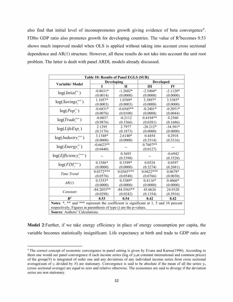
also find that initial level of incomepromotes growth giving evidence of beta convergence4.
FDIto GDP ratio also promotes growth for developing countries. The value of R2becomes 0.53
shows much improved model when OLS is applied without taking into account cross sectional
dependence and AR(1) structure. However, all these results do not take into account the unit root
problem. The latter is dealt with panel ARDL models already discussed.
Table 10: Results of Panel EGLS (SUR)
Variable/ Model Developing Developed I II III IV
log( )PC
iIntial -0.8631* (0.0014)
-1.2602* (0.0000)
-2.5404* (0.0000)
-2.1120* (0.0000)
log( )Ratio
itSavings 1.1057* (0.0003)
1.0769* (0.0003)
3.3897* (0.0000)
3.5385* (0.0000)
log( )Gr
itPop -0.6831* (0.0076)
-0.6545** (0.0100)
-0.2401* (0.0008)
-0.2051* (0.0044)
log( )Ratio
itTrade -0.0037 (0.9876)
-0.2112 (0.3366)
0.4194** (0.0381)
0.2560 (0.1686)
log( )itLifeExp 2.1295 (0.3176)
2.7977 (0.1873)
-28.212* (0.0000)
-34.581* (0.0000)
log( )Ratio
itIndustry 3.1348* (0.0000)
2.6140* (0.0000)
0.4454 (0.3514)
0.2918 (0.5316)
log( )PC
itEnergy -0.6623** (0.0440) -- 0.7607**
(0.0127) --
log( )Energy
itEfficiency -- 0.3693 (0.5398) -- -0.6942
(0.3528)
log( )Ratio
itFDI 0.3386* (0.0000)
0.3399* (0.0000)
0.0524 (0.3274)
0.0597 (0.2681)
Time Trend 0.0372*** (0.0576)
0.0365*** (0.0548)
0.0422*** (0.0766)
0.0678* (0.0030)
AR(1) 0.3353* (0.0000)
0.3389* (0.0000)
0.4116* (0.0000)
0.4066* (0.0000)
Constant -84.2053** (0.0298)
-84.5565** (0.0242)
45.0626 (0.1354)
24.9320 (0.3916)
R2 0.53 0.54 0.42 0.42 Notes: *, ** and *** represent the coefficient is significant at 1, 5 and 10 percent respectively; Figures in parenthesis of type () are the p-values. Source: Authors’ Calculations.
Model 2:Further, if we take energy efficiency in place of energy consumption per capita, the
variable becomes statistically insignificant. Life expectancy at birth and trade to GDP ratio are
4 The correct concept of economic convergence in panel setting is given by Evans and Karras(1996). According to them one would see panel convergence if each income series (log of yitat constant international and common prices) of the group(N) is integrated of order one and any deviations of any individual income series from cross sectional average(sum of yt divided by N) are stationary. Convergence is said to be absolute if the mean of all the series yit (cross sectional average) are equal to zero and relative otherwise. The economies are said to diverge if the deviation series are non stationary.

33
insignificant factors. FDI to GDP ratio, savings to GDP ratio, initial level of GDP per capita, rate
of growth of population and industry to GDP ratio are important factor in explaining the growth
process for developing countries.
Model 3:For developed countries with energy consumption per capita as one of the independent
varaibles, the results of this model show that by assuming cross-sectionaldependence and AR(1)
structure per capita energy consumption expendituretend to have a positive impact on growth of
per capita GDP. Among other variables, life expectancy at birth have negative and significant
impact, rate of growth of population, savings to GDP ratio, trade to GDP ratio and initial level of
per capita incomehave usual signs and are statistically significant. FDI to GDP ratio, industry to
GDP ratio and time component capturing growth rate of technology have insignificant impact at
5% level of significance.
Model 4: Finally, with energy efficiency, the results show that the effect becomes insignificant.
Trade to GDP ratio and FDI to GDP ratio also have insignificant impact while life expectancy at
birth, rate of growth of populationand initial level of per capita incomehave negative and
significant impact on growth.
4.2.3Growth Regressions Including CO2Emissions and an Interactive Term Further, growth regressions have been estimated by adding two additional variables such
as: CO2 emissions and an interaction term of CO2 emmisions and energy consumption per capita.
For this purpose, we consider two models. One, panel SURE model with AR(1) structure and
another being the panel ARDL model. We use the latter as there is unit root problem in almost
all the growth explanatory variables across country groups. Some variables are I(0) and some are
(1).
Table 11: Panel SUR Model Results
Developing Countries Dependent Variable: GDP Growth Per Capita

34
Variable Coefficient P Value Constant -11.2111 0.0524
log( )PC
iIntial -0.7422 0.0000
log( )Ratio
itIndustry 1.3252 0.0052
log( )Ratio
itFDI 0.4029 0.0000
log( )Ratio
itTrade 0.29991 0.1350
log( )Ratio
itSavings 1.8258 0.0000
log( )itLifeExp 3.8591 0.0062
log( )Energy
itEfficiency -0.2821 0.5043
log( )Gr
itPop -0.5354 0.0005 CO2 * Energy Consumption 0.4998 0.0446
log( )PC
itEnergy -1.7556 0.0019 Developed Countries
Constant 67.2571 0.0005 log( )PC
iIntial -2.4423 0.0000
log( )Ratio
itIndustry 0.6492 0.2087
log( )Ratio
itFDI 0.0119 0.8573
log( )Ratio
itTrade 0.8166 0.0001
log( )Ratio
itSavings 3.1606 0.0000
log( )itLifeExp -14.5239 0.0005
log( )Energy
itEfficiency 0.4501 0.4931
log( )Gr
itPop -0.1987 0.0035 CO2 * Energy Consumption 0.5979 0.0011
AR(1) 0.4234 0.0000 Transition Economies
Not Shown due to insignificant results Source: Authors’ Calculations
The results in Table 11 show that:
• In case of developing countries, Initial level of GDP per capita is negative and significant
in explaining growth per capita of developing countries. Log of industry/GDP, Log of
FDI/GDP, Log of Gross Savings/GDP, log of rate of growth of population and log of life
expectancyhave significant impact on growth per capita. Log of energy consumption per
capita tend to have negative and significant impact on growth per capita. Importantly log
of interactive term between energy consumption and co2 emissions tend to have positive
impact on growth per capita. The latter implying that as CO2 emissions increase, also
proxy for development in technologies which limit use of oil consumption and promotes

35
alternative use of energy resources like renewable, leads to decrease in the rate of
increase in energy consumption per capita, which in turn promotes growth per capita in
developing countries.
• In case of developed countries, we apply panel sure with AR(1) structure to data made
available for developed nations. Log of initial level of income, log of Trade/GDP, log of
Gross Savings/GDP, log of life expectancy, log of rate of growth of population and log of
interactive term(Co2 emissions with energy consumption per capita) have significant
impacts on growth per capita.
• In case of Transition economies, we are not presentingthe panel SURE model
results(with AR(1) structure of errors) as almost all variables in the regression model are
insignificant except CO2 emissions which have a negative impact and log of interactive
term which has positive and significant impact on growth per capita. The latter may be
due to the fact that transition economies may not have fully developed technologies that
can take care of limiting CO2 emissions. On the other hand interactive term is positive
may signify that people’s movement may have limited use of energy consumption per
capita in such countries, acknowledging that climate change is more due to anthropogenic
factors.
• We however reported two way random effects model results in case of transition
economies in Table 12. Unit root problem is present in almost all variables used in the
regression. We strangely find that in transition economies log of Gross Savings/GDP, log
of FDI/GDP and log of Trade/GDP have negative and significant impact on growth per
capita. This may be due to unit root and autocorrelation in error term. Also, non-market
forces play significant role for transition economies leading to false impact of such
variables(FDI, Trade and Savings) on growth per capita. Log of Industry/GDP, log of rate
of growth of population,log of energy consumption per capita, log of CO2 emissionsand
log of interactive term have significant impact on growth per capita of transition
economies.
Table 12: Random Effect Model Results
Transition Economies Dependent Variable: GDP Growth Per Capita

36
Variable Coefficient P Value Constant 390.4623 0.5490
log( )PC
iIntial 8.4212 0.7677
log( )Ratio
itSavings -2.4117 0.0000
log( )Gr
itPop -7.5824 0.0000
log( )Ratio
itTrade -91.5996 0.0000
log( )itLifeExp 216.1546 0.1329
log( )Ratio
itIndustry 51.3275 0.0005
log( )PC
itEnergy -171.6387 0.0000
log( )Ratio
itFDI -4.8554 0.0000
CO2 Emission -159.8203 0.0000 CO2 * Energy Consumption 30.0225 0.0000
Source: Authors’ Calculations
Panel ARDL Results The panel ARDL is the appropriate mode for studying long term and short term relationship
between variables when some variables are I(0) and some are I(1). The Table 13 shows long
term cointegrating coefficients along with short term ECM(Error Correction Model) coefficients.
The results show that:
• In case of developing countries, the long term results show that log of industry/GDP, log
of Trade/GDP, log rate of growth of populationand Log of energy consumption per
capitahave significant impact on growth per capita. The interactive coefficient of CO2
emissions and energy consumption per capita is positive but insignificant. The lagged
coefficient term in the ECM model is negative and significant implying that the gap
between actual and the long run value of dependent variable would be met at the speed of
82.7 %. The coefficient also indicates that there exists long term causality between
energy consumption per capita and the explanatory variables.
• In case of developed countries, The panel ardl results below of developed nations indicate
that log of industry value added/GDP, log of Trade/GDP(at 10% level of significance),
log of life expectancy(negative impact and significant) and log of rate of growth of
population(negative) have significant impact on grwoth per capita of developed nations.
Log of Energy consumption per capita and log of energy consumption*CO2 emissions
tend to have positive impact on growth per capita, although both variables are
insignificant factors.

37
• In case of transition economies, it seems that there is long run relationship among growth
and its explanatory factors. In this formulation the cointeq term in the short run equation
shows that the gap between actual and long run equilibrium value of the dependent
variable would be met at the speed of 34.8 %. This term is negative implying long run
causality between growth and its determinants. The long run equation shows Log of
Gross Savings/GDP, log of rate of growth of population, log of Trade/GDP, log of life
expectancy, log of energy consumption per capita, and log of FDI/GDP have significant
impact on growth per capita. Log of CO2 emissions(negative but insignificant) and log of
CO2 emissions * energy consumption per capita have positive impact on growth per
capita.
Table 13: Results of ARDL Developing Developed Transition
Long-Run Relationships Variable Coefficient P-Value Coefficient P-Value Coefficient P-Value
log( )Ratio
itIndustry 2.7897 0.0368 2.2587 0.0032 0.9790 0.6934
log( )Ratio
itFDI 0.6269 0.7597 -0.0967 0.3768 0.1947 0.0016
log( )Ratio
itTrade 1.5558 0.0163 0.6830 0.0930 10.4131 0.0000
log( )itLifeExp 2.1036 0.6550 -5.3469 0.0000 -4.8066 0.0803
log( )Gr
itPop -2.4344 0.0002 -0.3853 0.0000 0.5580 0.0175 CO2 * Energy Consumption 1.0834 0.2523 0.4746 0.3948 0.7317 0.3656
log( )PC
itEnergy -5.8810 0.0154 1.1180 0.2455 -2.9944 0.0795
log( )Ratio
itSavings 0.2867 0.6230 -- -- -0.7274 0.0002 CO2 Emissions -- -- -- -- -3.7745 0.5566
Error Correction Term COINTEQ -0.8277 0.0000 -0.6248 0.0000 -0.3487 0.0036
Source: Authors’ Calculations. 4.2.4 S-Shaped Relationship between Energy Consumption Per-Capita and Host of Explanatory Variables Our panel causality results indicate that the relationship may work the other way. Growth per
capita and its factors may impact log of energy consumption per capita. We hypothesize that the
relationship is S-shaped between energy consumption per capita and growth per capita GDP. The
latter would mean that first energy consumption increases at an increasing rate with an increase
in growth per capita and then after the point of inflextion is reached, energy consumption
increases but at a decreasing rate. The same relation is hypothesized between energy

38
consumption per capita and FDI/GDP, Trade/GDP and CO2 emissions(in metrics per tonne).
Mathematically, to prove for the S-Shape curve, we will assume the following model. Y is
energy consumption per capita while X can be either growth per capita, FDI/GDP or CO2
emissions or Trade/GDP. = exp ( − X )
log ( ) = − X
Taking first order derivative, we would get the following 1 =
=
= exp ( − X )
Taking second order derivative, we would get the following: = − 2
= exp ( − X ) − exp ( − X ) 2
= exp ( − X )( − 2 ) At the point of inflection, second order derivative would be 0, which would give: = 2
Therefore, any value less than X=b2/2 would give positive value for second order derivative ,
while for any value greater than X=b2/2, second derivative would be negative. This would imply
that the curve chnages its curvature from convexity to concavity implying s shaped relationship
between energy consumption per capita and host of its explanatory variables. Therefore, it is
hypothesized from step 2 of the above equation that log y is hypothesized to have negative
relationship with reciprocal of GDP per capita growth, reciprocal of Co2 emissions, reciprocal of
Trade/GDP and reciprocal of FDI/GDP. We first present the results for developing economies,
then transition and then finally of developed nations.We have panel data set for 18 developing
economies and we use data from 1980-2013 on our dependent variable and set of explanatory

39
variables. Panel unit Root tests(Levin,Lin,Chu and Imm Pesaran and Smith) have been
applied(not shown) and there is evidence of the unit root problem across the sample of
developed, transition and developed nations. It is assumed and tested that there is presence of
panel cross sectional contemporaneous correlations which allows us to use Panel SURE model
with error following AR(1) structure. We then finally use Panel ARDL model as all variables are
of I(0) and I(1) form. However, Panel ARDL results for S-shaped relationship between energy
consumption and its determinants are not robust for all three groups-developing economies,
transition economies and developed nations. Therefore, we do not show the panel ardl results.
The other results are shown in Table 14. The results show that:
• In case of developing countries, The results(panel SURE with AR(1) structure) indicate
that S-shaped relationship holds for CO2 emissions only for developing economies.
Energy Consumption per capita have Inverted S-shaped relationship for growth per
capita, FDI/GDP and Trade/GDP for set of developing countries considered in our study.
If one removes AR(1) assumption, all variables except FDI/GDP, have an S-shaped
relation with energy consumption per capita. Growth, Trade and FDI tend to increase
energy consumption at an increasing rate after the point of inflection has reached. Policy
makers need to address the issue by limiting energy consumption by focusing on
promoting usage of renewable energy.
• For developed nations, CO2 emissions and Trade/GDP have an S-shaped relation with
energy consumption per capita. If one removes the AR(1) structure on errors, all the
variables have an S-shaped relation with energy consumption per capita.
• For transition economies S-shaped relation with energy consumption per capita holds
with CO2 emissions only. In case assumption of AR(1) structure is removed we find
robust S-shape relation with growth per capita and CO2 emissions.
Table 14: Results for Looking S-Shaped Relationship
Dependent Variable: Energy Consumption Per Capita Variable Developing Developed Transition

40
Model Coefficient P-Value Coefficient P-Value Coefficient P-Value Constant 47.4158 0.8438 9.3047 0.0000 6.7227 0.0000
1/GDP Growth Per Capita 0.0002 0.2826 0.0001 0.0313 0.0003 0.8321
1/FDI to GDP Ratio 2.47E-05 0.0216 5.16E-06 0.2724 -5.13E-16 0.3771 1/Trade to GDP Ratio 0.4415 0.0244 -1.2369 0.0013 -0.2037 0.0000
1/CO2 Emissions -0.0258 0.0000 -3.8346 0.0000 0.0005 0.0895 AR(1) 0.9996 0.0000 0.9881 0.0000 0.9695 0.0000
Source: Authors’ Calculations.
All the results(based on panel sure and AR(1) error structure) indicate in common that with high
co2 emissions, it seems that there are concerted attempts made by national governments across
the countries and regional groups to develop technologies which can limit or reduce the rate at
which energy consumption grows in nation states. Panel ARDL results do not show any robust s
shape relationship between energy consumption per capita and its determinants.
5. Conclusions The present study is an attempt to evaluate the impact of energy consumption on
economic growth and economic growth on energy consumption for a set of developing,
transition and developed countries in the world. For this purpose, sample of 18 developing,18
developed and 16 transition countries have been considered to analyze the relationship between
variables. To pursue this, the study reports two types of results: one set of results consists of the
study of relationship between energy consumption per capita and rate of growth of GDP per
capita over the years; among others and in other set of results, S-shaped relationship between
energy consumption per capita and its determinants are examined for the set of developing,
developed and transition economies. The variables for growth regression are justified on the
basis of variant of Solow growth model as explained in the section 2.
Both the variables GDP per capita and energy consumption have unit root at level and are
stationary at first difference i.e. are I(1) for developing as well as developed countries panel
(which may have panel unit roots implying that despite all variables being I(1), one may not have
cointegration among variables in the developed nations). Energy consumption and GDP per
capita have a long term relationship in case of developing countries but no cointegrating
relationship in case of developed countries. However, as soon as we bring in some control
factors impacting growth, energy consumption has positive, significant and long term impact on
GDP per capita growth rates of developed nations but negative and significant long term impact
on growth per capita of developing countries.The developing countries, although trying to put

41
efforts in increasing expenditures in alternative energy sources (like non-renewable) oil
consumption still does not seem have many alternative sources of energy. Therefore, reducing oil
expenditure tends to promote growth among developing countries. Conspicuous consumption of
oil in cities (through purchase of multiple numbers of cars in one household) may also hinder
growth of GDP per capita, atleast in Indian cities. Energy efficiency tend to have positive but
insignificant impact on growth of GDP per capita for developed countries but significant impact
on growth of GDP per capita for developing countries. Panel ARDL results for studying
Cointegrating Relationship between growth and with CO2 emissions and interactive term,among
other variables show that with higher CO2 emissions, the rate at which energy consumption
grows declines which in turn promote growth across nations. The study strongly indicates that
CO2 emissions promotes technology for reducing energy consumption per capita by developing
environmentally friendly products which are renewable energy intensive products.
Further, panel VEC model in developing countries suggests that there is no short run
causality from per capita energy consumption to GDP per capita (with two variables only).
Causality from per capita GDP to energy consumption per capita is present in some of the
countries in short run as well as in long run. One possible reason for this result is that since the
countries are at different stage of development, some may be in secondary sector
(manufacturing), some in tertiary sector (services), they require different amount of energy in
their development process and hence growth doesnot really drive energy demand in all the
developing countries. Various phases of production and economic activities call for different
relations between per capita GDP and energy consumption. It may also be noticed that the
relation in question may not be a linear one - the initial phase of a developing country may
reflect an increasing relation between energy consumption and per capita GDP (since economic
activities are at large and use of consumer durables, particularly cooling machines, is on the rise)
but later, as pollution accumulates due to use of non-sophisticated technology, more efficient use
of energy and investment of the country in pollution abatement technology leads to energy
conservation. Same amount of energy may now produce more output leading to a falling apart of
the relation seen in the previous phase.
Moreover, Panel VAR model(based on two variables only) in developed countries
suggests that there is homogeneous non-causality in both the directions. This can be supported
by the argument that, since developed countries outsource their energy(involve themselves in
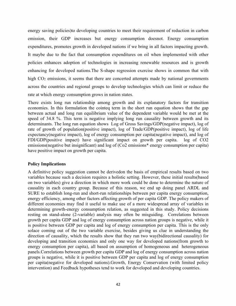
42
energy saving policies)to developing countries to meet their requirement of reduction in carbon
emission, their GDP increases but energy consumption doesnot. Energy consumption
expenditures, promotes growth in developed nations if we bring in all factors impacting growth.
It maybe due to the fact that consumption expenditures on oil when implemented with other
policies enhances adoption of technologies in increasing renewable resources and is growth
enhancing for developed nations.The S-shape regression exercise shows in common that with
high CO2 emissions, it seems that there are concerted attempts made by national governments
across the countries and regional groups to develop technologies which can limit or reduce the
rate at which energy consumption grows in nation states.
There exists long run relationship among growth and its explanatory factors for transition economies. In this formulation the cointeq term in the short run equation shows that the gap between actual and long run equilibrium value of the dependent variable would be met at the speed of 34.8 %. This term is negative implying long run causality between growth and its determinants. The long run equation shows Log of Gross Savings/GDP(negative impact), log of rate of growth of population(positive impact), log of Trade/GDP(positive impact), log of life expectancy(negative impact), log of energy consumption per capita(negative impact), and log of FDI/GDP(positive impact) have significant impact on growth per capita. log of CO2 emissions(negative but insignificant) and log of (Co2 emissions* energy consumption per capita) have positive impact on growth per capita.
Policy Implications A definitive policy suggestion cannot be derivedon the basis of empirical results based on two variables because such a decision requires a holistic setting. However, these initial results(based on two variables) give a direction in which more work could be done to determine the nature of causality in each country group. Because of this reason, we end up doing panel ARDL and SURE to establish long-run and short-run relationships between per capita energy consumption, energy efficiency, among other factors affecting growth of per capita GDP. The policy makers of different economies may find it useful to make use of a more widespread array of variables in determining growth-energy consumption relation, as suggested in this study. Policy decisions resting on stand-alone (2-variable) analysis may often be misguiding. Correlations between growth per capita GDP and log of energy consumption across nation groups is negative, while it is positive between GDP per capita and log of energy consumption per capita. This is the only solace coming out of the two variable exercise, besides giving us clue in understanding the direction of causality, which the results show that they run two way(bidirectional causality) for developing and transition economies and only one way for developed nations(from growth to energy consumption per capita), all based on assumption of homogeneous and heterogeneous panels.Correlations between growth per capita GDP and log of energy consumption across nation groups is negative, while it is positive between GDP per capita and log of energy consumption per capita(negative for developed nations).Growth, Energy Conservation (with limited policy intervention) and Feedback hypotheses tend to work for developed and developing countries.

43
References
1. Abosedra, S. &Baghestani, H. (1991). New Evidence on the Causal Relationship United
States Energy Consumption and Gross National Product. Journal of Energy and
Development. Vol. 14. 285-292.
2. Adjaye, A. J. (2000). The Relationship between Energy Consumption, Energy Prices and
Economic Growth: Time Series Evidence from Asian Developing Countries. Energy
Economics. Vol. 22(6). 615-625.
3. Akarca, A.T. & Long II, T.V. (1980). On the Relationship between Energy and GNP: A
reexamination. Journal of Energy and Development. Vol.5. 326-331.
4. Arellano, M. & Bond, S. (1991). Some Tests of Specification for Panel Data: Monte
Carlo Evidence and an Application to Employment Equations. The Review of Economic
Studies, Vol. 58(2). 277-297.
5. Barro, R.J. & Martin, X. S.I. (1995). Technology Diffusion, Convergence and Growth.
NBER working Paper, No. 5151.
6. Belloumi, M. (2009). Energy consumption and GDP inTunisia: Cointegration and
causality analysis. Energy Policy, Vol. 37 (2009). 2745–2753.
7. Breitung, J. (2000). The Local Power of Some Unit Root Tests for Pane Data. In:
Nonstationary Panels, Panel Cointegration, and Dynamic Panels, Baltagi, B.H. (Ed.),
Elsevier, Amsterdam, pp. 161-177.
8. Chiang, C. L. (2005). Energy consumption and GDP in developing countries: A
cointegrated panel analysis. Energy Economics. Vol. 27 (3). 415-427.
9. Choi, I. (2001). Unit Root Tests for Panel Data. Journal of International Money and
Finance. 20, 249-272.
10. Climate Institute (2013), Energy Efficiency and Economic
Growth,http://www.climateinstitute.org.au/verve/_resources/Vivid_Economics__Energy_
efficiency_and_economic_growth_June_2013.pdf
11. Cooper, W.W., Seiford, L.M. & Tone, K. (2007). Data Envelopment Analysis. A
Comprehensive Text with Models, Applications, References and DEA-Solver Software.
2nd Edition. Springer.

44
12. Dalei, N. N., (2016). Determinants of Energy Consumption in Open Economies.
GhoshDastidar, A., &Gupt, Y. (2016). Contemporary Issues in Trade, Environment and
Policy (pp. 89-104). New Delhi: Ane Books Pvt. Ltd.
13. Ekong, C. N., and E. L. Effiong. "Oil Price Shocks AndNigeriasMacroeconomy:
Disentangling The Dynamics Of Crude Oil Market Shocks". Global Business Review
16.6 (2015): 920-935. Web. 23 Jan. 2016.
14. Engle, R.F. & Granger, C.W.J. (1987). Co-Integration and Error Correction:
Representation, Estimation, and Testing. Econometrica, Vol. 55(2). 251-276.
15. Erdal, Z., Daigger, G. & Forbes, B. (2008). Energy Future: How To Bridge the Gap
between Energy Innovations and Sustainability Using a Whole System Approach. JRB08
- Energy Future Manuscript 122607.
16. Evans, P. &Karras, G. (1996). Convergence Revisited. Journal of Monetary Economics.
Vol. 37. 249-65.
17. Glasure, Y.U.( 2002). Energy and national income in Korea: further evidence on the role
of omitted variables. Energy Economics. Vol. 24. 355-365.
18. Greene, W.H. (2008). Econometric Analysis. Prentice Hall.
19. Hadri, K. (2000). Testing for Stationarity in Heterogeneous Panel Data. Econometrics
Journal. 3, 148-161.
20. Howland & Derek Murrow, ENE Lisa Petraglia& Tyler Comings (2009) ,Energy
Efficiency: Engine of Economic Growth : A Macroeconomic Modelling Assessment,
Economic Development Research Group, Inc,http://acadiacenter.org/wp-
content/uploads/2014/10/ENE_ExecSum_EnergyEfficiencyEngineofEconomicGrowth_F
INAL.pdf
21. Hurlin, C. &Venet, B. (2001). Granger Causality Tests in Panel Data Models with Fixed
Coefficients.http://basepub.dauphine.fr/bitstream/handle/123456789/6159/3F117993d01.
pdf?sequence=1.
22. Hurlin, C., Dumitrescu, E. (2012). Testing for Granger Non-causality in Heterogeneous
Panels.https://halshs.archives-ouvertes.fr/halshs-00224434/document
23. Im, K,S., Pesaran, M.H., Shin, Y. (2003). Testing for Unit Roots in Heterogenous Panels.
Journal of Econometrics 115, 53-74.
45
24. Johansen, S. (1988). Statistical Analysis of Cointegrating Vectors. Journal of Economic
Dynamics and Control. Vol. 12(1988). 231-254.
25. Jones, C.I. (2002). Introduction to Economic Growth. 2nd Edition. Norton & Company,
New York.
26. Kraft, J. & Kraft, A. (1978). On the Relationship between Energy and GNP. Journal of
Energy and Development. Vol. 3. 401-403.
27. Levin, A., Lin, C.F., Chu, C-S.J. (2002). Unit Root Tests in Panel Data: Asymptotic and
Finite Sample Properties. Journal of Applied Econometrics 108, 1-22.
28. MacKinnon, J.G., Haug, A. &Michelis, L. (1999). Numerical Distribution Functions of
Likelihood Ratio Tests for Cointegration. Journal of Applied Econometrics. Vol. 14(5).
563-577.
29. Maddala, G. S., & Wu, S. (1999). A Comparative Study of Unit Root Tests with Panel
Data and a New Simple Test. Oxford Bulletin of Economics and statistics. Vol. 61 (S1).
631-652.
30. Magazzino, C (2011). The relationship between CO2 emissions, energy consumption and
economic growth in Italy. International Journal of Sustainable Energy. 11/2014.
DOI: 10.1080/14786451.2014.953160.
31. Mankiw, N.G., Romer, D. & Weil, D. (1992). A Contribution to the Empirics of
Economic Growth. QJE. Vol.107(May). 407-438.
32. Masih, A. M. M., and Masih, R. (1996). Energy Consumption, Real Income And
Temporal Causality: Results From A Multi-Country Study Based On Cointegration And
Errorcorrection Modeling Techniques. Energy Economics 18 (3): 165-183.
33. Masih, M. M. &Masih, R. (1997). On the Temporal Causal Relationship between Energy
Consumption, Real Income and Prices: Some New Evidence from Asian-energy
Dependent NICs based on Multivariate Cointegration/Vector Error Correction Approach.
Journal of Policy Modeling. Vol. 19. 417-440.
34. Mathur, S.K., Arora, R., Ghoshal, I. and Singh, S. (2015). Domestic Energy Consumption
and Country’s Income Growth: A Quantitative Analysis of Developing and Developed
Countries using Panel Causality, Panel VECM, Panel Cointegration and SURE. Journal
of Quantitative Economics,DOI - 10.1007/s40953-015-0021-4.pp. 1-30.

46
35. Ozturk, I. (2010). A literature Survey on Energy – Growth Nexus. Energy Policy. Vol.
38. 340-349.
36. Pedroni, P. (1999). Critical Values for Cointegration Tests in Heterogeneous Panels with
Multiple Regressors. Oxford Bulletin of Economics and Statistics, Special Issue (1999).
0305-9049.
37. Pedroni, P. (2004). Panel Cointegration: Asymptotic and Finite Sample Properties of
Pooled Time Series Tests with an Application to the PPP Hypothesis. Econometric
Theory. Vol. 20. 597-625.
38. Pesaran, M. H. , Shin, Y. & Smith, R.J. (1999). Bounds Testing Approaches to the
Analysis of Long-run Relationships. Cambridge Working Papers in Economics. No.
9907. University of Cambridge.
39. Soytas, U. & Sari, R. (2003). Energy Consumption and GDP: Causality Relationship in
G-7 Countries and Emerging Markets. Energy Economics. Vol. 25. 33-37.
40. Squalli, J. (2007). Electricity consumption and economic growth: Bounds and causality
analyses of OPEC countries. Energy Economics. Vol. 29(6). 1192–1205.
Appendix Table
Table A1: List of Sampled Countries for the Empirical Analysis Developing Countries Developed Countries Transition Economies
Bangladesh Nigeria Australia Japan Albania Montenegro Chile Pakistan Austria Netherland Armenia Russian Federation
Colombia Peru Belgium New Zealand Azerbaijan Serbia Ghana Philippines Canada Norway Belarus Tajikstan
Hungary Saudi Arabia Finland Spain Bosnia Herzegovina Turkmenistan India Singapore France Sweden Croatia Ukraine
Indonesia Sri Lanka Hong Kong Switzerland Georgia Uzbekistan Kenya Thailand Ireland UK Kazakhstan
Malaysia Venezuela Italy USA Kyrgyz Republic Source: Authors’ Elaboration.