d:\usgs reports\authors\german\et finals\et eps finals\et4217

$: D:\USGS Reports\Authors\German\ET Finals\ET EPS Finals\ET4217$

U.S. GEOLOGICAL SURVEY

Water-Resources Investigations Report

Regional Evaluation of Evapotranspiration in the Everglades

00–4217

By Edward R. German

Tallahassee, Florida2000

U.S. DEPARTMENT OF THE INTERIOR

BRUCE BABBITT, Secretary

U.S. GEOLOGICAL SURVEY

Charles G. Groat, Director

Copies of this report can be purchased from:

U.S. Geological SurveyBranch of Information ServicesBox 25286Denver, CO 80225-0286800-ASK-USGS

The use of firm, trade, and brand names in this report is for identification purposes only and does not constitute endorsement by the U.S. Geological Survey.

For additional informationwrite to:

District ChiefU.S. Geological SurveySuite 3015227 N. Bronough StreetTallahassee, FL 32301

Additional information about water resources in Florida is available on theWorld Wide Web at http://fl.water.usgs.gov

Contents iii

CONTENTS

Abstract..................................................................................................................................................................................1Introduction ...........................................................................................................................................................................2

Purpose and Scope.......................................................................................................................................................2Description of the Study Area .....................................................................................................................................2

Data Collection and Determination of Evapotranspiration ...................................................................................................4Site Location and Instrumentation...............................................................................................................................4Data Processing and Screening....................................................................................................................................7Site Maintenance .........................................................................................................................................................7Calculation of Energy Terms .......................................................................................................................................8Calculation of Evapotranspiration ...............................................................................................................................9

Meteorologic Characteristics of the Everglades ....................................................................................................................11Rainfall ........................................................................................................................................................................11Incoming Solar Radiation............................................................................................................................................13Net Radiation...............................................................................................................................................................14Depth of Water.............................................................................................................................................................14Air and Surface-Water Temperature ............................................................................................................................14Vapor-Pressure and Air-Temperature Vertical Differences .........................................................................................15Evaporative Fraction....................................................................................................................................................15

Site-Specific and Regionalized Models of Evapotranspiration.............................................................................................15Availability of Data for Model Calibration .................................................................................................................15The Modified Priestley-Taylor Model .........................................................................................................................16Regionalization of the Modified Priestley-Taylor Models ..........................................................................................19

Regional Models Based on Measured Available Energy ..................................................................................23Regional Models not Based on Available Energy .............................................................................................23

Model Performance .....................................................................................................................................................25Evapotranspiration and Variation in Evapotranspiration in the Everglades ..........................................................................36Comparison of Turbulent Fluxes by Bowen-Ratio and Eddy-Correlation Methods .............................................................38Summary and Conclusions ....................................................................................................................................................47References .............................................................................................................................................................................48

FIGURES

1. Map showing the Everglades and locations of evapotranspiration (ET) stations ....................................................32. Photograph showing the open-water site in Loxahatchee National Wildlife Refuge ..............................................53. Photograph showing a vegetated site in Everglades National Park .........................................................................64. Diagram showing energy budget during daytime heating .......................................................................................8

5-25. Graphs showing:5. The relation between mean incoming solar radiation and mean net radiation, 1996-97 .................................146. Distribution of dead plant material at site 7, November 1996.........................................................................187. Cumulated measured evapotranspiration and simulated evapotranspiration using models based on

1996 data or 1997 data.....................................................................................................................................208. Simulation of Priestley-Taylor coefficient as a function of water level and incoming solar

energy for two selected levels of incoming solar energy.................................................................................249. Simulated daily evapotranspiration totals from site models and regional models, sites 1 and 2.....................26

10. Simulated daily evapotranspiration totals from site models and regional models, sites 3 and 4.....................2811. Simulated daily evapotranspiration totals from site models and regional models, sites 5 and 6.....................3012. Simulated daily evapotranspiration totals from site models and regional models, sites 7 and 8.....................3213. Simulated daily evapotranspiration totals from site models and regional models, site 9................................34

iv Contents

14. Median standard error for site models and regional models for the nine evapotranspiration sites, January 1996 through December 1997............................................................................................................ 35

15. Annual total measured and simulated evapotranspiration, January 1996 through December 1997 ............... 3616. Relation of mean annual evapotranspiration to water depth, January 1996 through December 1997............ 3617. Relation between mean annual evapotranspiration for 1996-97 and mean normalized difference

vegetation index for 1998................................................................................................................................ 3718. Range in monthly evapotranspiration at the nine sites, January 1996 through December 1997 .................... 3819. Hourly available energy, net radiation, and latent heat, February 4 and April 15, 1996 at sites 7 and 8........ 3920. Comparison of Bowen ratio from air-temperature and humidity differentials with Bowen ratios

from flux measurements from eddy-correlation measurements at site 7, June 22, 1998, through September 28, 1998......................................................................................................................................... 40

21. Comparison of latent heat calculated using Bowen ratios from air-temperature/humidity differentials with latent heat calculated using Bowen ratios from eddy-correlation measurements (site 7, June 22, 1998, through September 28, 1998).................................................................................................. 41

22. Relation of 30-minute turbulent flux to measured available energy, June 22, 1998, through September 29, 1999, at site 7 .......................................................................................................................... 43

23. Relation of daily mean turbulent flux to daily mean measured available energy, June 22, 1998, through September 29, 1999, at site 7 ............................................................................................................. 44

24. Comparison of measured available energy and turbulent flux from eddy correlation at 30-minute intervals, site 7, July 1 through July 14, 1998 ............................................................................... 45

25. Mean wind velocity for 15-minute intervals, site 7, July 1 through July 14, 1998......................................... 46

TABLES

1. Evapotranspiration-monitoring site characteristics ................................................................................................. 42. Site instrumentation................................................................................................................................................. 73. Summary of meteorological data for the evapotranspiration sites .......................................................................... 124. Number of data points used in model development ................................................................................................ 165. Summary of regression coefficients and goodness of fit for Priestley-Taylor site models ..................................... 186. Summary of regression coefficients and goodness of fit for site models of available energy ................................ 257. Model errors ............................................................................................................................................................ 358. Annual total measured and simulated evapotranspiration, January 1996 through December 1997 ....................... 35

Contents v

CONVERSION FACTORS, VERTICAL DATUM, ABBREVIATIONS, AND ACRONYMS

Temperature in degrees Fahrenheit (°F) may be converted to degrees Celsius (°C) as follows:°C = (°F-32)/1.8.

Altitude: In this report, altitude refers to distance above or below sea level.

Acronyms and additional abbreviations used in report:oC/m degree Celsius per meterET evapotranspirationENR Everglades Nutrient RemovalEROS Earth Resources Observation Systemsu* friction velocityg/cm3 grams per cubic centimeterg/m2-s grams per square meter per secondg/m2 grams per square meterin/mi inches per mileJ/oC-cm3 joules per degree Celsius per cubic centimeterJ/oC-kg joules per degree Celsius per kilogramJ/g joules per gramJ/g/oC joules per gram per degree CelsiuskPa/oK kilopascals per degree KelvinkPa/m kilopascal per meterλE latent heat fluxm/s meter per secondNIR near infraredNDVI Normalized Difference Vegetation IndexNOAA National Oceanic and Atmospheric AdministrationREBS, Inc. Radiation and Energy Balance Systems, Inc.SFWMD South Florida Water Management DistrictUSGS U.S. Geological SurveyVIS visible

Multiply By To obtain

Lengthinch (in) 2.54 centimeter (cm)foot (ft) 0.3048 meter (m)

mile (mi) 1.609 kilometer (km)

Areasquare foot (ft2) 0.0929 square meter (m2)

Massounce (oz) 28.349 gram (gr)

Energyjoule (J) 0.2388 calorie (cal)

Energy flux densitywatt per square meter (W/m2) 0.001433 calorie per square centimeter per minute (cal/cm2/min)

Flowinch per year (in/yr) 25.4 millimeter per year (mm/yr)

Pressure inches of mercury (in) 3.386 kilo Pascal (kPa)

pound per square inch (lb/in2) 68.95 millibar (mb)pound per square inch (lb/in2) 10.0 millibar (mb)

Speedmile per hour (mi/hr) 1.609 kilometer per hour (km/hr)

vi Contents

Abstract 1

Regional Evaluation of Evapotranspirationin the Evergladesby Edward R. German

ABSTRACT

Nine sites in the Florida Everglades were selected and instrumented for collection of data necessary for evapotranspiration-determination using the Bowen-ratio energy-budget method. The sites were selected to represent the sawgrass or cattail marshes, wet prairie, and open-water areas that constitute most of the natural Everglades sys-tem. At each site, measurements necessary for evapotranspiration (ET) calculation and modeling were automatically made and stored on-site at 15- or 30-minute intervals. Data collected included air temperature and humidity at two heights, wind speed and direction, incoming solar radiation, net solar radiation, water level and temperature, soil moisture content, soil temperature, soil heat flux, and rainfall. Data summarized in this report were collected from January 1996 through December 1997, and the development of site-specific and regional models of ET for this period is described.

Latent heat flux (λE) is the energy flux den-sity equivalent of the ET rate. Modified Priestley-Taylor models of λE as a function of selected inde-pendent variables were developed at each site. These models were used to fill in periods of miss-ing λE measurement, and to develop regional models of the entire Everglades region. The regional models may be used to estimate ET in wet prairie, sawgrass or cattail marsh, and open-water portions of the natural Everglades system. The models are not applicable to forested areas or to the brackish areas adjacent to Florida Bay.

Two types of regional models were devel-oped. One type of model uses measurements of

available energy at a site, together with incoming solar energy and water depth, to estimate hourly ET. This available-energy model requires site data for net radiation, water heat storage, and soil heat flux, as well as data for incoming solar radiation and water depth. The other type of model requires only incoming solar energy, air temperature, and water depth data to provide estimates of hourly ET. The second model thus uses data that are more readily available than the data required for the available-energy model.

Computed ET mean annual totals for all nine sites for the 1996-97 period ranged from 42.4 inches per year at a site where the water level is below land surface for several months each year to 57.4 inches per year at an open-water site with no emergent vegetation.

Although the density of photosynthetically-active plant leaves has been shown to relate directly to ET in some studies, it does not appear to relate directly to ET in the Everglades, based on comparison of annual ET data with leaf-area index, defined as the Normalized Difference Veg-etation Index (NDVI), data from satellite imagery. NDVI and ET appear to be inversely related in the Everglades. The greatest ET rates occurred at open-water sites where the NDVI data indicated the lowest leaf-area index. Among the remaining vegetated sites, there is no clear relation between ET and NDVI, though the highest ET rate corre-sponded to the lowest NDVI and one of the lowest ET rates corresponded to the highest NDVI value.

The variation in ET follows a seasonal pat-tern, with lowest monthly ET totals occurring in December through February, and highest ET

2 Regional Evaluation of Evapotranspiration in the Everglades

occurring in May through August. The greatest range in monthly ET among all nine sites for the 2-year period occurred at site 3: from 1.81 inches in December 1997 to 6.84 inches in July 1996.

A study to compare the Bowen-ratio/energy balance method of ET measurement with the eddy-correlation method was done at one site from June 22, 1998, through September 28, 1998. This comparison indicated that both methods gave comparable values of the Bowen ratio, but there was a considerable difference in available energy measured by the two methods. The mean of all 30-minute measured turbulent heat fluxes from the eddy-correlation apparatus for June 22 through September 29, 1998, was 137.4 watts per square meter, and the mean of the corresponding mea-sured energy was 163.6 watts per square meter, or about 20 percent greater. The disagreement in mean energy fluxes measured by the two methods is problematical and is not fully understood. Although the difference seems to be related to fric-tion velocity, and is practically non-existent at val-ues of friction velocity greater than 0.3 meter per second, the “correctness” of either method cannot be determined with the data available.

INTRODUCTION

Evapotranspiration is a major part of the hydro-logic cycle in Florida, particularly in the Everglades of South Florida. The water level is at or above land sur-face most of the year in most of the Everglades, and actual evapotranspiration (ET) approaches potential ET as determined by the availability of energy to drive ET. Rainfall is the largest quantity in the hydrologic cycle, but ET in wet areas may be almost as great as rainfall.

Solution of water-quality and quantity problems within the Everglades requires an understanding of the surface and subsurface flow systems. Evapotranspira-tion is a major component of the Everglades water bud-get (generally more than 40 inches per year) (in/yr) and is of crucial importance in developing this understand-ing. However, a regional, process-oriented understand-ing of evapotranspiration in the Everglades is lacking. As stated by Marjory Stoneman Douglas (1947), “it is the subtle ratio between rainfall and evaporation that is the final secret of water in the Glades.”

There is little information available to quantify the importance of ET in the hydrologic cycle. Evapora-tion pan data have been collected at some locations, but the pan data give only a limited understanding of actual ET. Recently, development of field data loggers and sensors have made it possible to determine ET using energy-budget methods (such as the Bowen-ratio method) or using direct measurements of water-vapor flux by methods such as the eddy-correlation method.

Purpose and Scope

This report presents ET values at nine sites within the natural Everglades system, for the period January 1996 through December 1997. These nine sites are in the freshwater non-forested parts of the Ever-glades, and do not include wetland tree islands, cypress heads, areas infested with melaleuca, hardwood ham-mocks, pinelands, mangrove swamps, or agricultural areas. The area represented by this study probably accounts for more than 90 percent of the region known as the natural Everglades.

Vertical differences in air temperature and in vapor-pressure, along with other meteorological data, were measured at 30-second intervals. These data were used in the Bowen-ratio method to determine ET at 30-minute intervals.

A modified Priestley-Taylor model was used to estimate ET during periods when data were unavailable or were judged to be too inaccurate for meaningful results. The models for the individual sites were inte-grated into a regional model, which may be used to esti-mate hourly ET at other locations in the Everglades as a function of incoming solar radiation and water depth.

Summaries of related micro-meteorological data are given in this report. These data show the range in micro-meteorological conditions that exist throughout the natural Everglades system during the period of study.

Description of the Study Area

The study area is within the natural Everglades area, which extends from south of Lake Okeechobee to the southern part of Everglades National Park (fig.1). This area is a wetlands system that is presently about 50 miles wide and about 100 miles long. The Everglades is regarded as unique in the world because it is not pri-marily associated with a natural river system, but is

Introduction 3

Figure 1. The Everglades and locations of evapotranspiration (ET) stations.


itself a wide and shallow “river” that transports water by sheet flow from Lake Okeechobee to the Gulf of Mexico. The slopes within this shallow “river” are gen-erally less than about 2 inches per mile (in/mi).

The Everglades contains several types of envi-ronments, which include freshwater marshes, tree islands, pinelands, mangrove swamps, coastal saline flats, and shallow coastal marine waters. This study is concerned with freshwater marshes, the predominant Everglades ecosystem. These marshes are character-ized by sawgrass stands of varying density and height, ranging from 2 or 3 feet (ft) above land surface to as high as 9 ft in some northern areas. Other common emergent plants in the freshwater marshes include spike rush, muhly grass, and in some areas, cattails. Extensive growths of cattails generally are located where phosphorus-rich waters from canals enter the Everglades, though relatively small stands of cattails occur in areas unaffected by phosphorus enrichment.

The annual rainfall in the Everglades is generally between 50-60 inches (in.), depending on location, with substantially more rainfall along the eastern edge (Lodge, 1994). The rainfall has a distinct seasonal pat-tern, with a wet season from May or June through Sep-tember or October that accounts for about 75 percent of the annual total. Water depths in the freshwater marshes range from 0 to 2 or 3 ft during the wet season. Mini-mum seasonal water levels generally occur in May before onset of the wet season; in particularly dry years, large portions of the Everglades may become dry and subject to wildfires. Heavy rainfall associated with tropical depressions, storms, and hurricanes can have a large impact on water-level conditions. A single such event can increase water levels by a foot or more over

large parts of the Everglades; because of the slow run-off rates, this can effect water levels for months.

DATA COLLECTION AND DETERMINATION OF EVAPOTRANSPIRATION

Nine sites were selected and instrumented for collection of data necessary for ET-determination and modeling. The Bowen-ratio energy budget method (Bowen, 1926) was selected for determining ET because all necessary data could be obtained using automatic equipment that could operate continuously in nearly all weather conditions. This method has been successfully used at other locations in Florida (Bidlake and others, 1993).

Site Location and Instrumentation

Sites were selected to provide a network repre-sentative of the non-forested portion of the Everglades ecosystem in terms of plant communities, duration of water inundation (hydroperiod), and geographic cover-age. Other factors in site selection were security and logistics. Sites in areas that are open to hunting and air boating were located in relatively remote locations and not on major air boat trails. Each site was located at the center of a circle of relatively uniform vegetative cover with a radius of at least 100 times the height of the upper air temperature/humidity sensor. Site locations and characteristics are listed in table 1, and the loca-tions are shown on the map in figure 1.

Table 1. Evapotranspiration-monitoring site characteristics

[Site numbers refer to fig. 1; THP refers to air temperature and humidity sensor]

Site Latitude/longitude Plant community

Height above land surface, in feet

CommentsVege-tation

Lower THP

Wind sensor

1 263910 0802432 Cattails 10 14 18 Considerable flow regulation, nutrient-rich water, abundant duckweed

2 263740 0802612 Open water 0 5 none

3 263120 0802011 Open water 0 4.7 8 Some lily pads at times

4 261855 0802257 Dense sawgrass 6.5 10 19

5 261530 0804417 Medium sawgrass 6 8.2 18 Dry part of some years

6 254443 0803011 Medium sawgrass 6 9 13

7 253659 0804208 Sparse sawgrass 5 7.7 14

8 252111 0803802 Sparse rushes 3 4 12 Dry part of each year

9 252135 0803146 Sparse sawgrass 3.5 5.3 12 Dry part of each year

Data Collection and Determination of Evapotranspiration 5

Stations were instrumented to provide data for: determination of total energy available for ET (latent heat flux, λE) and convection (sensible heat flux, H); determination of the Bowen ratio (the ratio H/λE), so that the amount of the total available energy that was utilized for ET could be determined; and characteriza-tion of meteorological conditions and ET-model devel-opment using ancillary data.

The array and arrangement of data sensors at the sites were dependent on whether the site was in open water or in dense, emergent vegetation. Examples of the two types of sites and their data-collecting equipment are shown in figures 2 (an open-water site) and 3 (a veg-etated site). The major difference between open-water sites and vegetated sites is the method of determining the air-temperature and humidity differential with height, which is necessary for computation of the

Bowen ratio. At the two open-water sites (sites 2 and 3), the air temperature and humidity differentials were measured from the water surface to a point 3-4 feet above the water surface. At the seven vegetated sites (sites 1, 4-9) the differentials were measured between two points in air, 3-5 feet apart.

At each site, sensor measurements (table 2) were made automatically every 30-seconds and these mea-surements were averaged and stored onsite at 15- or 30-minute intervals. These data were then transmitted daily by cellular telephone to computer storage in the office. Data were reviewed on a daily basis to detect equipment breakdown and sensor malfunction. Site visits were made at approximately monthly intervals for routine scheduled maintenance and cleaning, or more fre-quently when malfunctions occurred.

Figure 2. The open-water site in Loxahatchee National Wildlife Refuge.


Figure 3. A vegetated site in Everglades National Park (water-temperature sensors are located at water surface, mid-depth, and in bottom near stilling well). Soil temperature sensors, heat-flux plates, and soil-moisture sensors are located under net radiometers.


Table 2. Site instrumentation

[Sensor type: REBS, Radiation and Energy Balance Systems, Inc. Company names are given for sensor identification purposesonly and do not imply product endorsement by the USGS]

Data Processing and Screening

Data were collected from January 1996 through December 1997 for sites 1-8. Site 9, however, was installed in January 1997 to increase representation of drier parts of the Everglades; site 9 furnished data from January 1997 through December 1997. Only data that passed screening tests for accuracy were used to develop the models of ET. The screening tests were based on range limits, visual inspection of plotted net radiation, temperature and humidity readings to elimi-nate periods when sensors were obviously malfunc-tioning, and on criteria given by Ohmura (1982). Ohmura (1982) specified that flux calculations are inappropriate if the calculated latent heat flux is in the opposite direction from the observed vapor-pressure vertical difference. Such a situation would indicate an error in determination of either the energy budget or the vapor-pressure or temperature vertical differences. Ohmura (1982) also recommended that Bowen-ratio calculations be rejected if temperature or vapor-pres-sure vertical differences are at or less than sensor reso-lution limits. Resolution limits for this study are 0.013 degree Celsius for vertical temperature differ-ences and 0.003 kilopascal (kPa) for vapor-pressure differences. These screening criteria eliminated about

one-half of the available data from model development, mostly because of sensor failure and resolution limits. Most of the data rejected because of resolution limits or flux directions were for night-time hours, when energy inputs, air-temperature vertical differences, and vapor-pressure vertical differences are all relatively low.

Site Maintenance

Sites were visited at 4-6 week intervals for inspection and maintenance. Maintenance generally included the following items:

The net radiometer domes required the most fre-quent maintenance. These domes, made of soft trans-parent polyethylene, shield the sensors from moisture, wind, or debris that could affect sensor performance. Problems encountered included crushing by hail, peck-ing by birds, and gradual deterioration of the polyeth-ylene. Domes were changed at 3-month intervals, or sooner if damage occurred. If the domes were cracked, punctured, or there was evidence of water penetration into the sensor, the entire net radiometer was replaced.

Air temperature and humidity sensors failed fre-quently during the first year of operation, due to corro-sion of electrical contacts. A change in sensor design resulted in much-improved service life of these sensors during the second year of operation. The sensor exchange mechanisms were subject to occasional fail-ure, generally due to mechanical wear or water penetra-tion into the control circuitry.

Type of

measurement

Number of sensors

Sensor typeVege-tated sites

Open-water sites

Air temperature 2 1 Platinum resistance

Humidity 2 1 Resistance

Wind speed/direction 1 1 R.M. Young Model 05305

Incoming solar radia-tion (pyranometer)

1 1 LI-COR, Inc. LI-200

Net solar radiation 2 1 REBS, Inc. Q7.1

Water level 1 1 Float-driven potentiometer

Water temperature 2 2 Chromel-constantan thermocouples

Soil moisture content 3 0 REBS, Inc. SMP-2

Soil temperature 3 0 REBS, Inc. STP-1

Soil heat flux 3 0 REBS, Inc. HFT-1

Rainfall 1 1 Texas Electronic Model 525

Equipment Action

Ventilator fans Clean and replace, if not operating

Net radiometer domes Clean and replace, if damaged. Replace radiometer if water damaged

Radiation shields (air temperature and humidity)

Clean

Air temperature and humidity sensors

Clean, replace sensors, if necessary

Water-level sensor Raise float and check for proper response

Rain gage Check for obstructions, clear if necessary

Water temperature sensors

Check for proper position and reading

Net radiometers and pyranometer

Check for level, adjust if necessary

Sensor exchange mechanism

Check for smooth operation, replace as necessary


Calculation of Energy Terms

The energy budget is illustrated in figure 4 and defined in equation 1. In this equation, each term or product of terms represents an average energy flux over the specified time interval (30 minutes in this study).

, (1)

whereRn is the net solar radiation, in W/m2,G is the amount of energy passing through the

soil or involved with change in temperature

of the surface layer of soil, in W/m2,W is the amount of energy involved with change

in temperature of water standing on the land

surface, in W/m2,H is the sensible heat flux (heat transported by

convection), in W/m2,λ is the latent heat of vaporization of water,

in J/g,

E is the evaporation rate of water in g/m2-s, and the product λE is the latent heat flux, or heat

involved in vaporization or condensation of

water, in W/m2.

In equation 1, each term on the left of the equals sign is measured, and the left side of the equation rep-resents the total amount of energy available for latent heat and sensible heat (available energy). The sum of H and λE is the turbulent flux.

Net radiation (Rn) is measured directly by the net radiometers, but the measured value is affected by wind speed and must be corrected. Wind correction factor was calculated from wind measured at the sites using procedures described by C. Fritchen (REBS, Inc., writ-ten commun., 1995). The effect of wind is to lower the output from the net radiometer from the value that would be recorded in still air under the same radiative conditions. This effect increases with wind speeds up to about 9 miles per hour (mi/hr) and is nearly constant at wind speeds greater than 9 mi/hr. At these higher wind speeds, the effect of wind is to reduce the net radiome-ter reading by about 6 percent.

Soil heat flux (G) was measured at all vegetated sites, but was not measured at the open-water sites because these sites were always covered by water, gen-erally to a depth of more than 1 ft. At the vegetated sites, soil heat flux was determined from the sum of heat-flux measured by a heat-flux plate buried 5 centi-meters (cm) below the land surface and the change in heat stored in the soil profile above the plate. Calcula-

Rn G– W– H λE+=

Figure 4. Energy budget during daytime heating.


tion of the soil heat storage required measurement of average soil temperature in the soil column above the heat-flux plate, and also measurement of the moisture content of the soil in the same column. Average tem-perature was measured at the beginning of each time interval using a thermistor probe. Soil moisture was measured with a resistance-type sensor inserted into the soil profile. The change in soil heat storage for each 30-minute computation interval is given by the follow-ing equation (Campbell Scientific, 1990):

, (2)

where∆S is the change in energy in the soil above the

heat-flux plate, in W/m2,10,000 is a conversion factor between cm-2 and m-2,

∆Ts is the difference in average soil temperature for the 30-minute time interval, in oC,

Cs is the volumetric heat capacity of the soil, in J/oC-cm3,

d is the thickness of the soil layer (5 cm), and∆t is the time interval (1,800), in seconds.

The soil type at all sites was assumed to be a pre-dominately mineral medium sand, and the soil heat capacity was estimated from the relation:

, (3)

whereDb is the dry soil bulk density (assumed to be 1.5),

in g/cm3, Csd is the specific heat of the dry soil (assumed to

be 0.840 J/oC-g),Cw is the specific heat of water (4.190 J/oC-g), andXw is the mass-fraction of water in the soil

(g water/g dry soil).

Assumptions regarding soil properties have little effect on accuracy of the overall energy budget, because the soils are generally covered with water, and energy involved in temperature changes of the soil col-umn above the heat-flux plates is relatively small com-pared to other components of the energy budget. At site 8, which is dry 3-4 months each year, the average soil heat flux (G in eq. 1) was -1.4 watts per square meter (W/m2) for 1996-97, while the average total energy associated with Rn and W was 132 W/m2. At wetter sites, the magnitude of G, relative to the other terms, is

smaller. An estimate of sensitivity of ET calculation to soil properties was made for site 8, which is dry 3-4 months each year. At this site, changing the soil bulk density from 1.5 grams per cubic centimeter (g/cm3) to 1 g/cm3 resulted in a change of less than 0.5 percent in computed annual total ET.

Water heat storage (W) was calculated at all sites whenever water was standing on the land surface. Cal-culation of W required measurement of water depth and mean water temperature at the beginning and end of each calculation interval. The mean water tempera-ture was determined by averaging the surface-water temperature and the bottom-water temperature, deter-mined every 30 seconds, for 30-minute periods. The surface-water temperature was measured using a ther-mocouple mounted on the bottom of a float and was taken about 1 in. below the water surface. The bottom-water temperature was measured using a thermocouple fixed to the submerged land surface. Both thermocou-ples were mounted in the shadow of sun screens so they would not be heated directly by solar radiation. Water temperatures at the beginning of each 30-minute ET computational period were estimated by linear interpo-lation between the average temperatures for the preced-ing 15-minute period and the following 15-minute period. Water heat storage was calculated as:

, (4)

where ∆W is the change in heat storage in water, in

W/m2, 304,800 is the mass of water (g) in a 1 m2 section

1 foot deep,dw is the water depth, in feet,

∆Tw is the change in mean water temperature in the time interval, in oC,

Cw is the heat capacity of water (4.19), in J/g/oC, and

∆t is the time interval (1800), in seconds.

Calculation of Evapotranspiration

Although equation 1 indicates that the sum of λE and H is obtained by summing the components of the available energy, it does not by itself provide a means of distinguishing between the two. The energy sum can be apportioned between λE and H by measuring the Bowen ratio (B), which is defined as the ratio of H to λE.

S∆ 10 000, TsCsd∆ t∆⁄=

Cs Db Csd Cw Xw )+(=

W∆ 304 800 d, w TwCw∆ t∆⁄=


Bowen (1926) showed that B can be approximated as a function of vertical differences of temperature and vapor pressure in the air, or

, (5)

whereγ (known as the psychrometer constant) is

a function of air temperature and baro-metric pressure,

t2 and t1 are air temperatures measured at two points at different heights above the land surface, and

e2 and e1 are vapor pressures measured at the same two points.

Average values of the air-temperature differences (t2 - t1) and vapor-pressure differences (e2 - e1), taken every 30 seconds for a 30-minute period are used to determine Β. The energy budget (eq. 1) can then be solved for λE:

. (6)

Solution of equation 6 is not possible for inter-vals when Β = -1, because this would result in division by zero. Also, values of Β close to -1 will result in extreme values of the computed λE that are greatly affected by even small errors in the measured value of Β. To control this extreme dependency of λE on B when B is near -1, the value of B is constrained to exclude the interval from -0.7 to -1.3. This was done by setting B equal to -0.7 if the calculated B (eq. 5) is less than -0.7 and greater than -1.0, and setting B equal to -1.3 if the calculated B is less than or equal to -1 and greater than -1.3.

Several assumptions are involved in using the Bowen-ratio method. These include assuming one-dimensional heat and vapor flow, in the vertical direc-tion only. The method does not consider any heat or vapor transported to or from the measurement area from adjacent areas. For this reason, site selection requires a circle of uniform vegetative cover having a radius of at least 100 times the height of the midpoint between the two air temperature/humidity measure-ments. Another assumption is that eddy diffusivities for sensible heat (convection) and latent heat (water vapor) are equal and that these two fluxes originate from the same point on the land surface. At most sites, this is usually assured by making the lower air temperature/

humidity measurement at a height of 1.25 times the vegetative canopy height or greater (C. Fritchen, writ-ten commun., 1995). In the Everglades, this assump-tion of identical sources of sensible heat and latent heat probably is violated to some degree because of the presence of emergent vegetation and standing water at most sites. A disproportional amount of latent heat flux comes from the water surface, while a disproportional amount of sensible heat flux comes from vegetative material above the water surface that has been heated by solar radiation. This difference in source of heat fluxes could bias the Bowen-ratio measurement. Because the effective source of sensible heat may be higher than the effective source of latent heat, the mea-sured vertical air-temperature differential may be too large relative to the measured vertical water-vapor dif-ferential, thus biasing the calculated Bowen ratio to numbers greater than the true Bowen ratio. This posi-tive bias in Bowen ratio would result in a negative bias in measured ET. Discussion of an experiment to quan-tify the magnitude of this bias and effects of other assumptions is given in a later section of this report.

At vegetated sites (such as the one shown in fig. 3), the air temperature and vapor-pressure mea-surements necessary for the Bowen-ratio determination are made at two points several feet above the land sur-face and separated vertically by 3 to 5 ft. Because these differences may often be small in relation to sensor cal-ibration bias, it is necessary to use an averaging tech-nique to take into account the unknown sensor bias. The technique consists of determining average differ-entials of air temperature and vapor pressure between the higher and lower sensors for a 15-minute period from data measurements that are taken every 30 seconds, reversing the sensor positions, and deter-mining average differentials for another 15-minute period. By averaging the two differentials for the con-secutive 15-minute periods, an unbiased 30-minute average differential is obtained.

The averaging technique may be demonstrated as follows for two sensors, referred to as the right-hand sensor and the left-hand sensor. For the first 15-minute period, the right-hand sensor is above the left-hand sen-sor, and the unbiased average differential is:

, (7)

B γ t2 t1 )–( e2 e1–( )⁄=

λE Rn( G W )–– 1( B+⁄ )=

∆1 VRa1 VLa1– VRo1 bR– VLo1(– bL )–= =

Meteorologic Characteristics of the Everglades 11

where VRa1 is the actual mean value for the right-hand sen-

sor for the first time period,VLa1 is the actual mean value for the left-hand sen-

sor for the first time period,VRo1 is the observed mean value for the right-hand

sensor for the first time period,VLo1 is the observed mean value for the left-hand

sensor for the first time period,bR is the bias for the right-hand sensor, andbL is the bias for the left-hand sensor.

For the second 15-minute period, the sensors are reversed, so the unbiased average differential is:

, (8)

where the terms have the same meaning as in equation 7 except that they are for the second time period, as designated by the subscript 2.

The 30-minute average value of the two differen-tials ∆1 and ∆2 is given by:

(9)

where the sensor-bias terms bL and bR have dropped out, and ∆30 is expressed only in terms of observed (uncorrected for bias) averages for the two sensors. This technique assumes that the sensor biases are con-stant over the 30-minute period, but does not assume that the sensor biases are the same or are unchanged from one 30-minute time period to the next.

At open-water sites with little or no emergent vegetation (such as the one shown in fig. 2), the air-tem-perature and vapor-pressure differentials necessary for the Bowen-ratio determination are determined from measurements of water temperature at the water surface and air temperature and vapor pressure at a point 3 to 4 ft above the water surface. The water-surface temper-ature is measured by using a float-mounted thermocou-ple, and is assumed to represent the air temperature at the water-air interface. The vapor pressure at that point is assumed to be equivalent to 100 percent relative humidity. Because the differences between water surface and air are much greater than differences in the air over similar distances, the effect of air and vapor pressure sensor bias is negligible. Therefore, the sensor exchange mechanism is not required and only one air temperature/vapor pressure sensor is needed at such sites.

METEOROLOGIC CHARACTERISTICS OF THE EVERGLADES

Meteorological data from the nine sites are sum-marized in table 3 to indicate the range in conditions that occurred in the study area during 1996-97. The table shows the number of days of record during the 2-year period and summary statistics to depict the range in values of 30-minute averages of selected types of data. For rainfall, the summary indicates the number of days of record, maximum daily total rainfall, maxi-mum monthly total rainfall, and the total rainfall for the 2-year period. Site 9 was not operated during 1996, so data summaries for some characteristics that can vary considerably from year to year (such as rainfall and depth of water) may not be representative of the 2-year period summaries at sites 1-8.

Rainfall

Short-term rainfall (hourly or daily) probably is the most variable meteorological characteristic in the study area (table 3). Relatively small convective thun-derstorms can produce large amounts of rain within a small area. For example, on June 2, 1997, 6.0 in. of rainfall were recorded at site 8 before 10:30 a.m. Other sites south of Water Conservation Area 3 and within 20 miles or less of site 8 received much lower amounts during that morning (2.1 in. at site 9, 1.0 in. at site 6, and 0.6 in. at site 7). The maximum daily rainfall recorded during 1996-97 was 11.9 in. at site 8 on June 9, 1997. At that site, the 3-day total for June 8-10 was 15.2 in.

Maximum monthly rainfall totals and average annual totals also were quite variable among the sites. The maximum monthly rainfall ranged from 10.0 in. at site 5 to 26.1 in. at site 8. Average annual totals for the 2-year period ranged from 38.6 in. in 1996 at site 5 to 80.3 in. in 1997 at site 8. These data indicate that rel-atively large variations in annual rainfall can occur from one location to another within a year or two. These short-term variations are likely not related to site location, but rather are probably due to chance occur-rence of localized downpours. In any year, some loca-tions may receive much more or much less rain compared to the 50-60 in. long-term average (Lodge, 1994). All rainfall totals reported during this study probably are lower than actual rainfall, because tip-ping-bucket rain gages tend to under-measure rainfall during high-intensity events because of splashout of rain from the collector.

∆2 VLa2 VRa2 VLo2 bL– VRo2 bR )–(–=–=

∆30 ∆1 ∆2 ) 2⁄V( Ro1 VLo1 )– V( Lo2 VRo2 )–+[ ] 2⁄

=+(=


Table 3. Summary of meteorological data for the evapotranspiration sites

[N is the number of days of record; P5 is the 5th percentile, or value that was not exceeded 5 percent of the days; P95 is the 95th percentile, or value that was not exceeded 95 percent of the days; --, no data available]

Rainfall, in inchesIncoming short-wave radiation,

in watts per square meter

Site NMax daily

Max monthly

Total 1996

Total 1997

Site N P5 Mean Median P95

1 -- -- -- -- -- 1 719 0 192 7.5 806

2 -- -- -- -- -- 2 -- -- -- -- --

3 731 3.1 12.9 54.4 55.9 3 731 0 195 4.9 801

4 730 2.8 14.3 49.7 54.4 4 730 0 206 7.2 825

5 731 2.3 10.0 38.6 44.3 5 716 0 206 1.8 858

6 730 7.9 16.7 62.3 70.3 6 730 0 196 6.5 786

7 731 3.1 13.4 46.1 43.0 7 730 0 201 6.6 811

8 731 11.9 26.1 70.5 80.3 8 731 0 202 9.6 808

9 365 8.0 15.8 -- 46.7 9 349 0 199 8 792

Net radiation, in watts per square meter Depth of water, in feet

Site N P5 Mean Median P95 Site N P5 Mean Median P95

1 715 -48 125 -7.1 607 1 715 0.52 1.12 1.00 1.83

2 348 -71 122 -16 640 2 633 1.92 2.76 2.57 4.05

3 731 -70 121 -17 631 3 731 1.12 1.68 1.63 2.32

4 730 -43 133 -5.3 623 4 730 -.14 .66 .48 1.70

5 698 -43 132 -5.5 612 5 716 .30 .91 .91 1.71

6 730 -51 133 -9 638 6 730 .70 1.37 1.40 1.90

7 731 -51 131 -12 652 7 731 .60 1.34 1.46 1.99

8 731 -42 134 -6 622 8 731 -.85 -.06 .10 0.70

9 349 -50 139 -6 640 9 349 -.70 -.05 .00 0.50

Air temperature, in degrees Celsius Water temperature at surface, in degrees Celsiusa


1 730 12.2 22.7 23.3 31.2 1 730 18.5 25.5 26.1 30.6

2 634 13.0 22.7 23.4 30.1 2 634 16.1 24.4 24.7 32.3

3 731 13.9 23.5 24.3 30.2 3 731 16.7 25.7 26.0 34.0

4 730 12.6 23.0 23.8 31.1 4 640 13.6 23.8 24.9 30.7

5 716 11.5 22.5 23.4 31.3 5 716 14.3 23.1 23.6 30.2

6 730 14.0 23.7 25.0 31.0 6 730 16.3 24.6 25.4 30.8

7 730 14.6 24.0 24.8 30.9 7 730 17.4 25.7 26.0 32.8

8 731 13.5 23.6 24.5 31.3 8 410 15.8 25.9 26.8 34.5

9 349 15 23.7 24.0 31.0 9 161 19.0 27.6 27.9 33.9aSummaries only include days where water is above land surface

Meteorologic Characteristics of the Everglades 13

Incoming Solar Radiation

Incoming solar radiation depends only on atmo-spheric transparency, time of day, day of year, and lati-tude, and thus, is independent of site characteristics such as vegetative cover and water level. The range in lati-tude from the northern-most site (site 1) to the southern-most site (site 8) is about 1.3 degrees, and is not in itself large enough to result in a large difference in solar radi-ation. Latitude variation in mean solar radiation on a horizontal plane at the top of the atmosphere is about 7 W/m2/degree at 25o N latitude in December, and about 2 W/m2/degree in June (interpolated from solar radia-tion data for latitude 30o N and latitude 20o N, Brutsaert, 1991). Over the entire study area, this north-south vari-

ation is about 9 W/m2 in December and about 3 W/m2 in June.

The mean incoming solar radiation for all seven sites at which incoming solar radiation was measured during 1996-97 was 200 W/m2, and ranged from 192 W/m2 (site 1) to 206 W/m2 (site 5) (table 3). This range is within about 3 percent of the mean for all seven sites. The major factor related to incoming solar radia-tion in the study area is cloud cover, and the observed differences in incoming solar radiation are probably related mostly to differences in cloud cover during the 2-year period. Although there could be areal patterns of cloud cover that might be related to latitude, prevailing wind direction, distance from the ocean or other factors, such a pattern is not apparent from this study.

Table 3. Summary of meteorological data for the evapotranspiration sites--Continued

[N is the number of days of record; P5 is the 5th percentile, or value that was not exceeded 5 percent of the days; P95 is the 95th percentile, or value that was not exceeded 95 percent of the days; --, no data available]

Vapor-pressure differences, in kilopascals per meterb Air-temperature differences, in degrees Celsius per meterc


1 488 -0.0385 -0.005 -0.006 0.032 1 521 -0.403 -0.024 -0.021 0.321

2 633 -2.07 -.79 -.64 -.053 2 631 -5.40 -1.74 -1.87 2.23

3 730 -2.48 -.96 -.76 -.12 3 729 -5.480 -2.253 -2.400 1.300

4 468 -.042 -.005 -.008 .045 4 506 -.376 .016 .020 0.492

5 546 -.055 -.012 -.012 .033 5 574 -.387 -.030 -.026 0.323

6 491 -.038 -.010 -.010 .022 6 510 -.264 -.040 -.037 0.201

7 480 -.036 -.012 -.012 .011 7 478 -.209 -.052 -.041 0.089

8 652 -.066 -.010 -.012 .054 8 662 -.58 -.031 -.035 0.547

9 284 -.052 -.010 -.013 .046 9 296 -.544 -.046 -.030 0.447bSummaries do not include differences less than 0.003 kilopascals cSummaries do not include differences less than 0.013 degrees

Evaporative fraction, in percentdAvailable energy,

in watts per square meter

Site N P5 Mean Median P95 Site N Mean Median

1 251 26 66 68 170 1 715 125 49

2 539 64 84 82 109 2 348 117 86

3 728 58 81 79 118 3 731 121 99

4 338 34 69 64 140 4 730 132 42

5 351 44 78 70 152 5 698 133 57

6 316 38 71 70 126 6 730 133 43

7 329 51 79 74 129 7 731 131 88

8 535 32 71 67 138 8 731 132 40

9 244 32 62 63 110 9 349 138 18dEvaporative fraction is the percent of the measured available energy that is accounted for by latent heat. Summaries are for data that have passed screening


Net Radiation

Net radiation is the difference between incoming solar and longwave radiation and outgoing longwave and reflected solar radiation. Although incoming radi-ation is mainly a function of cloud cover, air tempera-ture, and air moisture content and would be nearly constant over the study area on a cloudless day, outgo-ing radiation depends on reflective and thermal proper-ties of the land surface and the vegetative cover. Thus, in contrast to incoming solar radiation, net radiation can vary from site to site.

The mean annual net radiation recorded at all eight sites at which net radiation was recorded during 1996-97 was 129 W/m2, and ranged from 121 W/m2 at site 3 to 134 W/m2 at site 8 (table 3). (At site 9, the mean net radiation for 1997 was 139 W/m2, but the site was not operating in 1996.) This range among the eight sites is within about 5 percent of the mean for all eight sites, and is thus of similar magnitude to the range in incoming solar radiation. A plot of annual incoming solar radiation and mean net radiation for 1996-97 (fig. 5) shows evidence of a weak relation between the two quantities, but the relation is not statistically signif-icant at the 5 percent probability level. This implies that the relation between incoming solar radiation and net radiation is affected to some degree by site charac-teristics, although the effect is not great.

Although incoming solar radiation is near zero at night, net radiation is negative because at night, long-wave radiation from the vegetation, land, and water surface generally exceeds incoming long-wave radiation from the atmosphere. The most negative night-time net radiation values occurred at the open-water sites, as indicated by the 5th percentile (P5) net radiation values in table 3 (-70 at site 3 and -71 at site 2).

Depth of Water

The median water depths above land surface at sites 1-8 operated during 1996-97, ranged from 0.1 ft (site 8) to 2.57 ft (site 2) (table 3). Median water depth at site 9 during 1997 was 0 ft. Water level was some-times below land surface at sites 4, 8, and 9.

Air and Surface-Water Temperature

The mean air temperatures for 1996-97 were all within a range of 1.5 oC, ranging from 22.5 oC at site 5 to 24.0 oC at site 7 (table 3). The higher mean tem-peratures were at the southern-most sites (sites 6-9), although the mean water temperature at site 3 (in the northern part of the study area) was nearly as high as at the southern-most sites. There is more of a north-to-south pattern in lower temperatures (see 5th percentile (P5) of air temperatures in table 3) than in higher tem-peratures, perhaps indicating that warm-season tem-peratures are about the same over the entire area, but that cool-season temperatures are substantially lower in the north part of the area than in the south part. Because the lowest temperatures occur generally at night, this areal difference in P5 air temperatures may result from a difference in night-time cloud cover over the area. Clear skies generally are associated with lower night-time air temperatures than occur during cloudy nights.

Water-surface temperatures were more variable among the sites than were air temperatures. Mean water temperature for 1996-97 ranged from 23.1 oC at site 5 to 25.9 oC at site 8. Mean water temperature for 1997 at site 9 was 27.6 oC. Factors affecting water-surface temperature could include water depth and thickness of vegetative cover, as well as air tempera-ture and solar radiation.

Figure 5. The relation between mean incoming solar radiation and mean net radiation, 1996-97. (Data for site 9 are for 1997.)

Site-Specific and Regionalized Models of Evapotranspiration 15

Vapor-Pressure and Air-Temperature Vertical Differences

Mean vapor-pressure vertical differences at open-water sites (sites 2 and 3) were much larger in magnitude than at the vegetated sites (table 3). The dif-ference in these vertical differences is probably caused by the difference in sensor positioning. At the open-water sites, vertical differences in vapor-pressure (and air temperature) were measured close to the water sur-face (between the water surface and a point about 4 ft above the water surface), rather than between two points in air. Gradients in vapor pressure and air tem-perature are greatest near the water-or-land surface and decrease with height above land surface. Among the vegetated sites, the mean vapor-pressure vertical differ-ences ranged from -0.005 kilopascal per meter (kPa/m) (sites 1 and 4) to -0.012 kPa/m (sites 5 and 7). The neg-ative sign of the mean vertical difference indicates that vapor pressure generally decreased with altitude, a con-dition necessary for evaporation to occur. Reverse dif-ferences (vapor pressure increasing with altitude) occurred at least 5 percent of the time at all vegetated sites, indicating periods of dew formation. At the open-water sites, reverse differences occurred less than 5 percent of the time, and less frequently than at vege-tated sites.

Like vapor-pressure vertical differences, mean air-temperature vertical differences at open-water sites (sites 2 and 3) were much larger in magnitude (-1.74 oC/m and -2.25 oC/m, respectively) than at the vegetated sites (table 3). At the vegetated sites, the mean air-temperature vertical differences ranged from -0.052 oC/m (site 7) to 0.016 oC/m (site 4).

Evaporative Fraction

The evaporative fraction (Ef) is defined as the percent of the measured available energy that is accounted for by latent heat. The mean Ef at the open-water sites (sites 2 and 3) was more than 80 percent, and at the vegetated sites ranged from 62 to 79 percent (table 3). These Ef values indicate that evaporation is generally more important in heat transport than is con-vection. At certain times, however, convection is more important than evaporation, especially at vegetated sites, as indicated by the 5th percentile values (P5) of Ef. The P5 value of Ef ranged from 26 to 51 at the vege-tated sites (sites 1 and 4-9), indicating that at times con-

vective heat transport is more important than latent heat transport.

SITE-SPECIFIC AND REGIONALIZED MODELS OF EVAPOTRANSPIRATION

Models of latent heat as a function of selected independent variables were developed at each site. These models were used to fill in periods of missing latent-heat measurement, and to develop a regional model of the entire Everglades region.

Availability of Data for Model Calibration

The 30-minute means of latent heat calculated from energy budget data and Bowen-ratio determina-tions that met the screening procedures described pre-viously were used to calibrate individual site models relating the available energy to latent heat. The site models express latent heat as a function of water level, incoming solar radiation, and available energy. Table 4 summarizes the quantity of acceptable data available for the model calibration.

Records used for model calibration must include acceptable data for the dependent variable (latent heat) and all of the independent variables (available energy, incoming solar radiation, and water level). At all sites, the quantity of acceptable data used in model calibra-tion is considerably less than the total data collected. For example, at site 1, the 2 years of data collection amounted to 35,088 intervals (30-minute) of data col-lection, but the total number of records used in model calibration was only 12,039, or about 34 percent.

Another criterion used to exclude data from model development was restriction of the range in latent heat values to exclude extreme values. All aver-age latent heat measurements that were greater than 500 W/m2 or less than -100 W/m2 in a 30-minute inter-val were considered to be outliers that are not represen-tative of normal conditions and that could have a disproportionately large effect on model calibration. These outliers could occur during intervals with Bowen ratios near -1, or during intervals when turnover or wind-induced mixing of water causes a relatively large change in water temperature that affects the water heat storage term W in equation 1. Values of latent heat in the excluded range generally accounted for less than 3 percent of the total number of latent heat measure-ments used in model calibration.


Most of the independent-variable data (energy, incoming solar energy, and water level) were suitable for use in model calibration. An exception was site 2, where problems associated with roosting birds caused more than half of the net radiation measurements to be discarded. Birds landing on the sensors often changed sensor orientation from the level position, and often damaged the sensor shields or changed the transpar-ency of the shields. At other sites, the greatest amount of rejected data was for vapor-pressure vertical differ-ence and temperature vertical difference data that are needed to determine the Bowen ratio. These data were often rejected, either because the differences were less than the limits of accurate measurement for the sensors, or because vapor-pressure vertical differences were in the opposite direction from the latent-heat flux. Both of these conditions generally occur at night or on cloudy days when solar energy input is relatively low. Either vapor-pressure difference or temperature-difference data were rejected about 20-40 percent of the time at vegetated sites, but less than 10 percent of the time at open-water sites (sites 2 and 3). Since both of these measurements are necessary for determination of the Bowen ratio, the number of Bowen ratios usable for determination of latent heat were generally about 35 to

60 percent of the total number of measurements at the vegetated sites, and about 75 to 90 percent of the total number of measurements at the open-water sites (sites 2 and 3).

The Modified Priestley-Taylor Model

The Priestley-Taylor model of potential evapora-tion (Priestley and Taylor, 1972) is a relatively simple model that has been successfully applied in many areas. This is a semi-empirical model, in that it is derived from the physics-based Penman-Monteith model (Monteith, 1965) that expresses ET as a function of available energy, vapor-pressure deficit, air temper-ature, pressure, aerodynamic resistance (a function of primarily wind speed, and plant-canopy height and roughness), and canopy resistance (a measure of resis-tance to vapor transport from plants). In the Priestley-Taylor model, the atmosphere is assumed to be satu-rated, in which case the aerodynamic term is zero. In actuality, atmospheric saturation generally does not occur. Therefore, an empirical multiplier is applied (the Priestley-Taylor coefficient) as an empirical correction to account for the fact that the atmosphere does not generally attain saturation.

Table 4. Number of data points used in model development

[N is the total possible number of data points, or the number of 30-minute intervals monitored; available energy is the sum of net radiation, soil heat flux, and change in heat storage in water and soil; Vp gradient is the vertical vapor-pressure differential in air; T gradient is the vertical temperature differential in air]

Site N

Number of “good” data points

Independent variablesData necessary for

determination of latent heatAvail-able

energy

Incom-ing

solar

Waterlevel

Vp gradient

T gradient

Bowenratio

Total in

model

1 35,088 34,315 34,509 34,318 23,417 24,988 12,040 12,039

2 35,088 16,733 34,175 30,393 30,361 30,293 25,879 12,255

3 35,088 35,087 35,087 35,086 35,055 34,980 30,671 30,671

4 35,088 35,038 35,038 35,038 22,485 24,307 15,254 15,254

5 35,088 33,502 34,366 34,366 26,188 27,549 16,819 16,104

6 35,088 35,038 35,038 35,038 23,586 24,480 15,182 15,182

7 35,088 35,037 35,031 35,087 23,047 22,953 15,807 15794

8 35,088 35,086 35,086 35,086 31,277 31,795 21,205 21,205

9 16,800 16,746 16,746 16,746 13,640 14,232 10,323 10,323


The form of the Priestley-Taylor equation is:

, (10)

where λ is the latent heat of vaporation of water, in J/g,

E is the evaporation rate, in g/m2-s,the product λ E is the latent heat flux, or energy

used for evapotranspiration, in W/m2,α is the Priestley-Taylor coefficient (dimension-

less),∆ is the slope of the saturation vapor-pressure

curve, in kPa/oK, A is the available energy (sum of net radiation,

soil heat flux, and change in heat storage in water), in W/m2, and

γ is the psychrometric constant computed from atmospheric pressure and air temperature (Fritschen and Gay, 1979), in kPa/oC.

The range in atmospheric pressure is small, and a con-stant value of 101 kPa was used to calculate γ.

Priestley and Taylor (1972) estimated that the value of α was 1.26 over a free-water surface or a dense, well watered canopy. Other studies have exam-ined use of a modified form of the Priestley-Taylor equation, in which the value of α is varied according to soil-water availability (Davies and Allen, 1973), sensi-ble heat flux (Pereira and Villa Nova, 1992), or solar radiation (De Bruin, 1983). De Bruin (1983) noted that the diurnal variation in α primarily is related to solar radiation. Sumner (1996) studied ET in a ridge area of Central Florida and developed a Priestley-Taylor model in which α was expressed as a function of solar radiation, vapor-pressure deficit, soil moisture, and a sinusodial function of the julian day to take into account seasonal factors such as plant cycles. Use of this model to fit measured ET was as good as the fit obtained using the more rigorous Penman-Monteith model. Knowles (1996), in a study of ET in the Rain-bow Springs and Silver Springs basins in north-central Florida, used a function relating α to net radiation, air temperature, and leaf-area index.

Preliminary work in developing Priestley-Taylor models for the Everglades sites involved trials of vari-ous models of α as a function of independent variables including water level, air temperature, vapor-pressure deficit (the difference between atmospheric moisture content at saturation and actual atmospheric moisture content), wind speed, incoming solar radiation, and a harmonic term with a period of 1 year. The harmonic term was intended to account for any seasonal effects

not included in the other independent variables. With the exception of wind speed, all of the independent variables tried in the α models were significant at a 5-percent level in explaining variation in measured latent heat. Many of the independent variables contrib-uted little to the accuracy of the predicted latent heat. The most significant terms in the model of α were water level and incoming solar radiation, and these terms were selected for formulation of all site models. Inclusion of the other variables caused little gain in pre-diction accuracy, and resulted in a more complex model requiring availability of more independent data.

Priestley-Taylor models of 30-minute ET totals for all of the Everglades sites were developed in which α was expressed as a linear function of incoming solar energy and water level, resulting in the following model:

,(11)

whereλ, E, ∆, A, and γ are the same as in equation 10, C0, C1, C2 and C3 are a unique set of constants for

each site,S is depth of water above land sur-

face (negative if below land surface), and

Rs is incoming solar radiation, in W/m2.

The values for C0, C1, C2 and C3 are determined by expanding equation 11 and using least-squares regres-sion. All available data for 1996-97 were used to deter-mine these values.

Regression statistics and values for the coeffi-cients (table 5) indicate goodness-of-fit characteristics and some common attributes among the nine site mod-els. In all cases except one (site 1), site model coeffi-cients of determination were 0.85 or greater. At site 1, the lower coefficient of determination (0.73) could be related to varying site characteristics, such as presence or absence of duckweed, and variation in amount of dead cattail debris. The model coefficients of variation ranged from 23 percent at site 9 to 52 percent at site 1.

Both water level (S) and incoming solar radia-tion (Rs) were significant at the 95-percent level in explaining variation in latent heat at all sites. The signs of the regression coefficient C1 indicate that for a selected amount of available energy, both α and latent heat increase as S increases. The coefficient C2 and C3 indicate that, at vegetated sites (all sites except 2 and 3), α initially decreases as Rs increases, and then as Rs

λ E α ∆ A ∆ γ )+(⁄=

λ E C0 C1S C2Rs C3Rs2 ) ∆ A ∆ γ )+(⁄+ + +(=


exceeds values ranging from about 800 W/m2 to 2,000 W/m2, α increases as Rs increases. At open-water sites (sites 2 and 3), α initially increases as Rs increases, and then, at site 3, decreases at Rs values greater than 600 W/m2.

Table 5. Summary of regression coefficients and goodness of fit for Priestley-Taylor site models

[N is the number of records used in the regression. C0, C1, C2, and C3 are the regression coefficients in the relation λ E = (C0 + C1 S + C2 Rs + C3 Rs

2) ∆ A/ (∆+γ); S is the water depth in feet; Rs is the incoming solar radiation in watts per square meter; R2 is the coefficient of determination; and C.V. is the coefficient of variation]

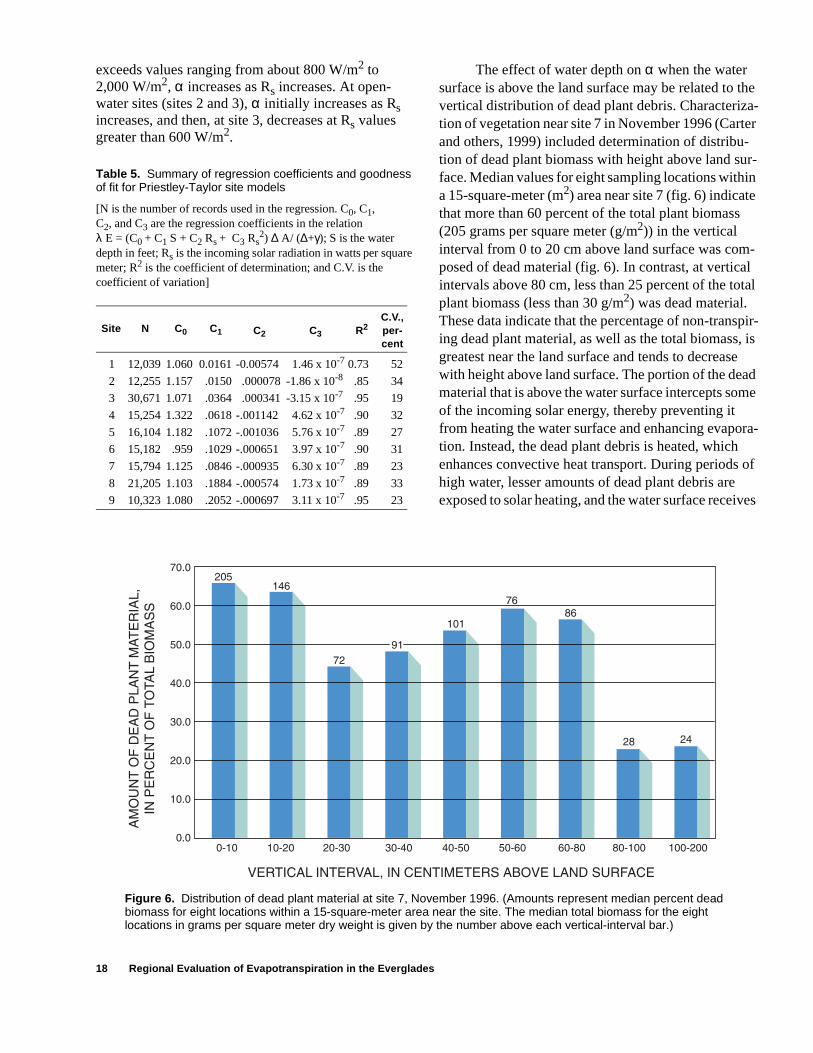
The effect of water depth on α when the water surface is above the land surface may be related to the vertical distribution of dead plant debris. Characteriza-tion of vegetation near site 7 in November 1996 (Carter and others, 1999) included determination of distribu-tion of dead plant biomass with height above land sur-face. Median values for eight sampling locations within a 15-square-meter (m2) area near site 7 (fig. 6) indicate that more than 60 percent of the total plant biomass (205 grams per square meter (g/m2)) in the vertical interval from 0 to 20 cm above land surface was com-posed of dead material (fig. 6). In contrast, at vertical intervals above 80 cm, less than 25 percent of the total plant biomass (less than 30 g/m2) was dead material. These data indicate that the percentage of non-transpir-ing dead plant material, as well as the total biomass, is greatest near the land surface and tends to decrease with height above land surface. The portion of the dead material that is above the water surface intercepts some of the incoming solar energy, thereby preventing it from heating the water surface and enhancing evapora-tion. Instead, the dead plant debris is heated, which enhances convective heat transport. During periods of high water, lesser amounts of dead plant debris are exposed to solar heating, and the water surface receives

Site N C0 C1 C2 C3 R2C.V., per-cent

1 12,039 1.060 0.0161 -0.00574 01.46 x 10-7 0.73 52

2 12,255 1.157 0.0150 0.000078 -1.86 x 10-8 0.85 34

3 30,671 1.071 0.0364 0.000341 -3.15 x 10-7 0.95 19

4 15,254 1.322 0.0618 -.001142 04.62 x 10-7 0.90 32

5 16,104 1.182 0.1072 -.001036 05.76 x 10-7 0.89 27

6 15,182 0.959 0.1029 -.000651 03.97 x 10-7 0.90 31

7 15,794 1.125 0.0846 -.000935 06.30 x 10-7 0.89 23

8 21,205 1.103 0.1884 -.000574 01.73 x 10-7 0.89 33

9 10,323 1.080 0.2052 -.000697 03.11 x 10-7 0.95 23

Figure 6. Distribution of dead plant material at site 7, November 1996. (Amounts represent median percent dead biomass for eight locations within a 15-square-meter area near the site. The median total biomass for the eight locations in grams per square meter dry weight is given by the number above each vertical-interval bar.)


a greater portion of the solar energy than during periods of lower water. As a result, the portion of solar energy that is transformed into latent heat may be directly pro-portional to the water level, as is indicated by the posi-tive value of the stage coefficient (C1 in table 5) at all sites.

When the water level is below land surface, as occurred occasionally at sites 8 and 9, α is still related directly to water level. This is probably because mois-ture availability at the land surface decreases as the water level declines.

The relation of α to Rs is more complex, and at vegetated sites changes from an inverse relation between α and Rs at Rs values of about 800 W/m2 or greater to a direct relation at relatively high values of Rs. At site 3 (an open-water site), the relation between α and Rs is direct for Rs values of about 600 W/m2 and changes to inverse for higher Rs values. This relatively complex nature of the functional relation between α and Rs is because Rs and other variables related to α, such as air temperature and vapor-pressure deficit, are interrelated. As a result of these interrelations, it is not possible to offer a simple explanation for the relation between α and Rs.

Although the final site and regional models are calibrated using all data for January 1996 through December 1997, the sensitivity of the model calibration to time period of the calibrating data was examined by determining the regression coefficients for two sets of data: 1996 data and 1997 data. Then, cumulative sums of measured ET, simulated ET using the model cali-brated with 1996 data, and simulated ET using the model calibrated with 1997 data were plotted for each site (fig. 7). The cumulative sums of measured and sim-ulated ET include only time intervals for which ET measurements were of acceptable accuracy based on the screening techniques described previously.

The plots indicate that the fit of the 1996 and 1997 models to measured ET was within about 2 inches per year (about 8 percent or less). For example, at site 7, the accumulated measured ET (including only peri-ods passing screening criteria) was 31.3 in. in 1996. The corresponding total ET simulated using the 1996 model was 30.9 in., or about 1.3 percent less than the measured value. The total ET for 1996 that was simu-lated using the 1997 model was 30.0 in., or about 4.2 percent less than the measured value.

At other sites, particularly site 1, the model cali-bration was more dependent on the time period. At site 1, the difference between total simulated ET using the

1997 model and total measured ET in 1996 was about 6 in., or about 32 percent. The difference between total measured ET in 1996 and ET simulated using the 1996 model, however, was much less (about 1.79 in. or 9.6 percent less than the measured total), although the difference is still relatively great compared to corre-sponding differences at other sites. The reason for the difference between the 1996 and 1997 models is not known, but may be the result of flow regulation at the site. Water levels and discharge through the site 1 area varied frequently in response to inflow and outflow control that was necessary for maintenance and opera-tion of the Everglades Nutrient Removal (ENR) project of the South Florida Water Management District (SFWMD). This control of flow through the area could have affected the energy balance by introducing an energy source (water that was warmer or cooler than ambient water) that was not considered in the measure-ment of available energy at the site. Thus, the accuracy of the energy budget could have varied because of flow regulation, with the result that model calibration error is greater at site 1 than at other sites.

Regionalization of the Modified Priestley-Taylor Models

The individual site models of ET were combined and used to formulate regional models for estimating ET in wet prairie, sawgrass or cattail marsh, and open-water portions of the natural Everglades system. The models are not applicable to forested areas or to the brackish areas adjacent to Florida Bay.

Two types of models were developed. One type uses measurements of available energy at a site, together with incoming solar energy and water depth, to estimate hourly ET. This available-energy model requires site data for net radiation, water-heat storage, and soil-heat flux, as well as data for incoming solar radiation and water depth. The other type of model requires only incoming solar energy, air temperature, and water depth data to provide estimates of hourly ET. The second model uses data that are more easily obtainable than the data required for the available-energy model, but does not provide as accurate an esti-mate of ET.


Figure 7. Cumulated measured evapotranspiration and simulated evapotranspiration using models based on 1996 data or 1997 data. (Plots include only time intervals for which evapotranspiration measurements passed accuracy-screening tests.)


Figure 7. Cumulated measured evapotranspiration and simulated evapotranspiration using models based on 1996 data or 1997 data. (Plots include only time intervals for which evapotranspiration measurements passed accuracy-screening tests.)--Continued


Regional Models Based on Measured Available Energy

The presence of some common attributes among the individual Priestley-Taylor models (table 5) indi-cates that a generalized form of the model could pro-vide a reasonable estimate of ET at all sites. This would indicate that a generalized (regional) model would be appropriate for estimating ET at areas in the Everglades that had characteristics similar to the sites modeled in this project.

The simulated values of α from the expression (C0 + C1S + C2Rs + C3 Rs

2 ) in equation 11 is plotted for all sites in figure 8, for solar intensities of 200 and 800 W/m2. The range in stage plotted for each site is from the 5th percentile to the 95th percentile (table 3). The plots indicate that, at 200 W/m2, the relations of α to stage are similar but not identical among the sites. For the five vegetated sites (1, 4, 5, 6, and 7) that are never or only occasionally dry and with a mean water depth greater than 0.5 ft, sites 4 and 6 define the upper and lower boundaries of the relation. Sites 4 and 6 are characterized by dense or medium sawgrass, and the reasons for the resultant differences in the α to water-level relation are not obvious. At higher solar-energy levels (800 W/m2), the plots of α as a function of water level define two obvious groups: open-water sites (2 and 3) and vegetated sites (all others). The large sepa-ration between the two site types (open water and veg-etated) at the higher energy level indicates that a substantial portion of the incoming solar energy at veg-etated sites is used in heating plants and plant debris, with a resultant relative increase in sensible heat trans-port compared to latent heat transport.

A generalized relation of α to water level and incoming solar energy was developed for vegetated and open-water sites by using least-squares regression to fit a data set of α generated by the individual site models. The values of α were generated over a range of water levels between the 5th- and 95th-percentile water levels at each site (table 3) in 0.1-ft intervals, and a range of incoming solar radiation values from 0 to 1,200 W/m2 in 100-W/m2 intervals. The functional relation used in the regression was:

, (12)

where S and Rs have been defined previ-

ously, and C0, C1, C2, C3, and C4 are constants determined by

least-squared regression.

The values of the five regression constants in equation 12 are:

These two generalized relations are shown in figure 8 for incoming solar energy levels of 200 and 800 W/m2. The goodness-of-fit of the generalized vegetated-site model to specific sites depends on the incoming energy level. For example, the generalized vegetated-site model underestimates α for site 4 at 200 W/m2, but overestimates α for the same site at 800 W/m2. The generalized open-water site model seems to fit both sites (2 and 3) at all incoming energy levels.

Regional Models not Based on Available Energy

Regional models of ET were developed in which the available energy for a 30-minute period (A in eq. 10) is estimated from solar radiation, air tempera-ture, and water depth, and the Priestley-Taylor coeffi-cient (α) is estimated from equation 12.

The first step in developing the regional model not requiring measurement of available energy was to develop site models of ET in which the available-energy term (A) is replaced by Aest, which is formu-lated as follows:

, (13)

where Aest is the estimated available energy, in W/m2,

Rs has been defined previously, C0, C1, and C2 are constants determined by least-

squares regression, and

, (14)

whereW is a surrogate for heat storage in water, in

W/m2, 709.5 is the quantity 304,800 Cw/∆t for ∆t of 1,800 seconds (see eq. 4),

S has been defined previously,Tair is the mean air temperature for the previous

15 minutes, in oCelsius, andT2.5 is the mean air temperature for the previous

2.5 hours, in oCelsius.

α C0 C1 S C2 S2

C3Rs C4 Rs2

+ + + +=

Site type C0 C1 C2 C3 C4

Vegetated 1.1263 0.1156 -0.0271 -0.000821 03.95 x 10-7

Open water 0.9613 0.1362 -0.0182 0.000177 -1.07 x 10-7

Aest C0 C1Rs C2W+ +=

W 709.5 S Tair T2.5 )–(=


Figure 8. Simulation of Priestley-Taylor coefficient as a function of water level and incoming solar energy for two selected levels of incoming solar energy. (Relations plotted are for mean values of water level and incoming solar radiation in 30-minute intervals.)


The rationale for equation 13 is that the net radi-ation term in the equation for available energy is replaced by a linear function of incoming solar radia-tion, and the water heat-storage term is replaced by a surrogate quantity in which the change in air tempera-ture from a 2.5-hour mean air temperature is used to represent change in water temperature during the 30-minute period. The 2.5-hour time period was selected because it provided the best overall fit for equation 13 compared with other time intervals that were evaluated (0.5, 1, 1.5, 2, 3, 4, 5, and 10 hours).

Regression statistics and values for the regres-sion constants are given in table 6. The coefficient of determination was 0.90 or higher at four of the nine sites, and was lowest at sites 2, 3, and 7. These three sites generally have the deepest water (of the nine sites), and the water heat storage term is thus relatively large. Small fluctuations in water temperature due to wind, rain, and convection can result in a relatively large amount of noise in the water heat storage term, and thus a relatively large error in relations between available energy and predictor variables. The sum of this noise tends to approach zero over a time span of several hours.

Table 6. Summary of regression coefficients and goodness of fit for site models of available energy

[N is the number of records used in the regression. C0, C1, and C2 are the regression coefficients in the relation Aest = C0 + C1 Rs + C2 708.5 S (Tair - T5); where Aest is the estimated available energy in watts per square meter; Rs is the incoming solar radiation in watts per square meter; S is the water depth in feet; Tair is the air temperature, in degrees Celsius; T5 is the mean air temperature for the previous 2.5 hours, in degrees Celsius; R2 is the coefficient of determination; and C.V. is the coefficient of variation]

Generalized relations for Aest were derived by combining the individual site models of Aest, as was done for the generalization of α. This was done using least-squares regression to fit a data set of Aest values generated by the site models given in table 6. The val-ues of Aest were generated over a range of incoming solar radiation values from 0 to 1,200 W/m2, water lev-els from -1 to 4 ft, and air-temperature differences (Tair - T2.5) from -7 to 7 oCelsius. The functional rela-tion used in this generalization was the same as that used for the individual site models of Aest (eq. 13). The values of the three regression constants representing the regionalized version of equation 13 are:

Model Performance

Fit of simulated daily ET from site and regional models is shown for each site in figures 9-13. The site models (top plot in each set of plots for a site) generally produce simulated daily ET totals that are unbiased over the range in daily ET, but at some sites the site models tend to under-predict for days with relatively high ET totals. This bias is most noticeable for site 5 (fig. 11), and probably indicates that the relation of α to environmental factors is more complex than the rela-tion used in equation 11. At site 5, the bias could result in simulated daily ET totals that are 10-15 percent lower than actual ET for some days with relatively high ET rates. Overall, this bias probably will not affect annual total ET values or monthly totals for seasons with relatively low ET rates, because these longer time periods will contain relatively few high-ET days.

The regional site models using measured energy tend to overestimate daily ET at sites 1, 2, 3, and 6 (fig. 9, 10, and 11), and tend to underestimate daily ET at sites 5 and 8 (fig. 11 and 12). The regional site models without measured energy generally have more scatter in the fit of daily ET totals, and in some cases are noticeably biased. The bias is most notable for sites 7 and 8 (fig. 12). For these two sites, daily ET is overes-timated at relatively low ET rates, and is underesti-mated at high ET rates.

Site N C0 C1 C2 R2C.V. per-cent

1 4,290 -20.73 0.7565 0.0776 0.87 50

2 4,386 20.16 .4948 .0613 .54 132

3 2,093 -6.98 .6567 .1176 .79 60

4 4,380 0.7247 .6432 .0293 .94 29

5 4,190 11.39 .5923 .0436 .92 32

6 4,380 -8.66 .7213 .0479 .89 42

7 4,382 41.87 .4459 .0364 .70 49

8 4,385 3.064 .6382 .1546 .96 24

9 2,093 -5.02 .7204 -.0064 .98 19

Site type Co C1 C2

Vegetated 5.171 0.6311 0.0506

Open water 78.26 0.2165 0.0654


Model errors are summarized in table 7, which lists standard errors of residuals (the difference between measured and simulated ET) for 30-minute totals, daily sums, and monthly sums from the site models and regional models. The model errors gener-ally are largest for the 30-minute ET simulation, and

smallest for monthly sums. The smallest standard errors were for site models, and the largest errors were for regional models without available energy. For site models, standard errors were generally in the 20 to 30 percent range for 30-minute ET sums, in the 8 to 14 percent range for daily sums, and within the 3 to

Figure 9. Simulated daily evapotranspiration totals from site models and regional models, sites 1 and 2.


7 percent range for monthly sums. Regional models with available energy performed nearly as well as the site models, with standard errors that were generally within the 20 to 34 percent range for 30-minute ET sums, within 10 to 16 percent range for daily sums, and

within 3 to 11 percent for monthly sums. Standard errors for the regional models without available energy were larger, generally in the 30 to 90 percent range for 30-minute ET sums, within 15 to 30 percent for daily sums, and within about 7 to 12 percent for the monthly sums.

Figure 9. Simulated daily evapotranspiration totals from site models and regional models, sites 1 and 2.--Continued


REGIONAL MODEL WITHOUT

MEASURED ENERGY

REGIONAL MODEL WITH

MEASURED ENERGY

SITE MODEL: SITE 7

SIM

UL

AT

ED

EV

AP

OT

RA

NS

PIR

AT

ION

,IN

INC

HE

S

0

0.3

0.1

0.2

0

0.3

0.1

0.2

0

0.3

0.1

0.2

0 0.30.1 0.2

MEASURED EVAPOTRANSPIRATION, IN INCHES

0 0.30.1 0.2

0.30 0.1 0.2

LINE OF EQUALITY



Figure 13. Simulated daily evapotranspiration totals from site models and regional models, site 9.


Table 7. Model errors

Table 8. Annual total measured and simulated evapotrans-piration (ET), January 1996 through December 1997

[Measured ET includes estimates of ET made using individual site models for periods when a Bowen ratio could not be calculated. The regional model with measured energy simulates ET as a function of available energy (sum of net radiation and water and soil heat storage), water level, and incoming solar radiation. The regional model with simulated energy simulates ET as a function of water level, incoming solar radiation, and air temperature]

Comparison of the median values of the standard errors at the nine stations (fig. 14) indicates that, over-all, the standard error of the regional model with avail-able energy is nearly as low as the error for the individual site models, regardless of the summation period. Simulation of 30-minute ET with the regional model without energy, however, is much less precise than simulation of 30-minute ET with the other models. For monthly summations of ET, all three models pro-duce results with similar precision, though the regional model without energy is the least precise of the models.

Mean annual ET and ET simulated by the models generally agree within about 2 in/yr (table 8 and fig. 15). The greatest differences between measured and modeled ET occurred for site 1, where the mean annual ET simulated by the regional model with measured energy was nearly 3 in. greater than the measured ET, and the ET simulated by the regional model with simu-lated energy was nearly 4 in. greater than measured ET. The relatively large error at site 1 may be related to reg-ulation of flow through the area. This flow regulation could have affected the energy balance by introducing an energy source (water that was warmer or cooler than ambient water) that was not considered in the measure-ment of available energy at the site. Thus, the accuracy of the energy budget could have been variably affected by the flow regulation, with the result that model cali-bration error is greater at site 1 than at other sites.

Site ModelModel error, in percent of mean

30-minute

Daily Monthly

1 Site 52 28 20Regional type 1 56 30 23Regional type 2 66 31 21









Site

Average annual ET, inches

Measured

Regional model with measured

energy

Regional model with simulated

energy

1 42.9 45.7 46.82 57.4 56.5 54.63 53.1 54.0 55.94 46.2 45.4 46.95 49.6 47.9 48.56 46.6 48.5 48.27 51.2 50.4 49.08 43.5 42.1 41.69 42.4 42.5 41.4

Minimum 42.4 42.1 41.4Maximum 57.4 56.5 55.9

Median 46.6 47.9 48.2

Figure 14. Median standard error for site models and regional models for the nine evapotranspiration sites, January 1996 through December 1997.


EVAPOTRANSPIRATION AND VARIA-TION IN EVAPOTRANSPIRATION IN THE EVERGLADES

Computed ET annual totals for all nine sites, over the 2-year period from January 1996 through December 1997, ranged from 42.4 in/yr at site 9 to 57.4 in/yr at site 2 (table 8 and fig. 15). The computed ET was greatest at the open-water sites: site 2 (57.4 in/yr) and site 3 (53.1 in/yr). Among the nearly always-wet vegetated sites (sites 1, 4, 5, 6, and 7), ET was lower, ranging from 42.9 in/yr (site 1) to 51.2 in/yr (site 7), with an average value of approximately 47 in/yr. The ET computed at site 1 is low in compari-son to the ET at other nearly always-wet vegetated sites. This relatively low ET is due in part to a tendency for more cloud cover at site 1 during the study period, as indicated by comparing the average level of incom-

ing solar radiation at site 1 (192 W/m2) with the aver-age for the other sites (201 W/m2). This difference in solar energy input could account for about 5 percent of the difference in ET between site 1 and the other vege-tated sites, or about 2.3 in/yr. Among the other wet-vegetated sites (4, 5, 6, 7), ET ranged from 46.2 to 51.2 in/yr. The ET at the two sites where the water level was below land surface at least several weeks each year was substantially lower than at all other sites and was 42.4 in/yr at site 9 and 43.5 in/yr at site 8.

The variation in annual ET among the nine sites appears to relate at least partially to water depth (fig. 16). At two sites (sites 1 and 6), however, annual ET was lower than at other sites with similar median water depths. The reason for these lower values has not been determined, but at site 1 it may be related to flow regulation and shading of the water surface by dead plant debris and prolific growths of duckweed that sometimes occurred.

To assess the relation of annual ET rate to differ-ences in living plant leaf density among the sites, a set of data from National Oceanic and Atmospheric Administration (NOAA) polar-orbiting satellites was used to characterize annual mean and variation in green-vegetation density at the ET sites. The data used are referred to as NDVI, which is a measure of the “greenness” of reflectance from the earth’s surface.

Figure 15. Annual total measured and simulated evapotranspiration, January 1996 through December 1997.

Figure 16. Relation of mean annual evapotranspiration to water depth, January 1996 through December 1997.

Evapotranspiration and Variation in Evapotranspiratoin in the Everglades 37

Data are available from the Earth Resources Observa-tion Systems (EROS) Data Center of the U.S. Geolog-ical Survey (USGS) as averages of 2-week intervals at a resolution of 1 square kilometer (km2). For this assessment, data available from 1998 were used, though the ET data are for 1996-97. This difference in time period is probably not significant for comparing NDVI characteristics among the sites because the sites change little from year to year, except when the areas of interest are subject to wildfire. No fires were known to have occurred near any of the ET sites during the period 1996-98.

The NDVI is calculated from the difference of near-infrared (NIR) and visible (VIS) reflectance val-ues divided by the sum of NIR and VIS. This normal-ized difference produces values in the range of -1.0 to 1.0, where increasing positive values indicate increas-ing green vegetation and negative values indicate non-green (non-vegetated) surface features such as water, barren land, or clouds. The NDVI index is then com-puted by scaling the normalized difference to the range of 0 to 200, where computed -1.0 equals 0, computed 0 equals 100, and computed 1.0 equals 200. As a result, NDVI values less than 100 represent clouds, water, and other non-vegetative surfaces; values equal to or greater than 100 represent vegetative surfaces.

The resolution of the NDVI data is insufficient to characterize the sites to the same scale as the ET mea-surement fetch, so the correspondence between the NDVI area and the measured ET area is not exact. This problem is especially evident at the open-water sites, where the extent of open water is sufficient to satisfy the fetch requirements for operation of the ET sites, but is only a small percentage of the 1 km2 resolution of the NDVI data. For this reason, the NDVI of the open-water sites was taken from data for Lake Okeechobee in Florida (fig. 1), where an NDVI value could be selected to represent only open water. The NDVI for these open-water sites was generally about 90 NDVI units during each 2-week period of 1998.

Although the density of photosynthetically active plant leaves has been shown to relate directly to ET in some studies (Sumner, 1996; Stannard, 1993), it does not appear to relate directly to ET in the Ever-glades. The NDVI and ET seem to be inversely related in the Everglades. The greatest ET rates occurred at open-water sites (sites 2 and 3) where the NDVI was estimated to be 90 units (fig. 17). Among the vegetated sites, there is no clear relation between ET and NDVI, though the highest ET rate corresponded to the lowest

NDVI (site 7) and the second lowest ET rate corre-sponded to the highest NDVI value. At sites 8 and 9, the low ET rate was probably due to lack of standing water during several months, and not to any relation between ET and NDVI. At vegetated sites with stand-ing water, a denser vegetative cover may inhibit evap-oration from the standing water surface and promote the transport of sensible heat due to heating of dead plant debris, so that ET rates are inversely proportional to NDVI or any other measure of plant cover.

The variation in ET follows a seasonal pattern, with lowest monthly ET totals occurring in December through February, and highest ET occurring in May through August (fig. 18). The monthly total ET among all nine sites for the 2-year period ranged from 1.81 in. at site 1 in December 1997 to 6.84 in. at the open-water site 3 in July 1996. The maximum range within a month among the nine sites was in April 1996, when the monthly total ranged from 2.82 in. at site 8 to 5.78 in. at site 2. The average water level at site 8 was about 0.75 ft below land surface in April 1996. This low water table is probably the principal reason for the low ET at site 8.

Figure 17. Relation between mean annual evapotranspiration for 1996-97 and mean normalized difference vegetation index (NDVI) for 1998. (NDVI is from satellite image data.)


Hourly net radiation, available energy, and latent heat are plotted for sites 7 and 8 (fig.19) for 2 days selected to represent a range in water-level and meteo-rological conditions. On February 4, 1996, the passage of a cold front caused air and water temperatures to fall sharply during the day at both sites. Storage of heat in the standing water provided energy for evapotranspira-tion at relatively high rates, even during pre-dawn and post-dusk periods, especially at site 7. Differences in shape of the latent-heat curves at the two sites on Feb-ruary 4 probably are related to the difference in water depths. The water depth at site 7 was about 1.7 ft, and at site 8 was about 0.2 ft. The presence of deeper water at site 7 tended to buffer solar input of energy and pro-vided a relatively large and constant source of energy. At site 8, with shallower water, the buffering action of the water was less, so that night-time ET rates are rela-tively low and daytime ET rates are relatively high compared to site 7. Also, with more total energy stored in the water column at site 7, which was released as the cold front passed, the average 24-hour latent heat was substantially greater (about 160 W/m2 at site 7 com-pared to about 110 W/m2 at site 8).

The effect of water availability on ET is shown by comparison of latent heat fluxes at the two sites on April 15, 1996 (fig. 19). On that date, the water level at site 8 was about 0.6 ft below land surface, and the water level at site 7 was about 0.7 ft above land surface. The evaporative fraction at site 8 was substantially lower

than at site 7. This difference in energy partitioning is probably because water standing above the land sur-face is more readily available for evaporation than is water below the land surface. The effect of energy storage in water is shown by the continued evapotrans-piration of water at site 7, even after sundown. Evapo-transpiration at site 8 ceased at sundown.

COMPARISON OF TURBULENT FLUXES BY BOWEN-RATIO AND EDDY-CORRELA-TION METHODS

As noted in an earlier section of this report, use of the Bowen-ratio method involves several assump-tions, including identical sources of latent and sensible heat, and insignificant heat storage in the plant canopy. To assess possible effects on ET related to these assumptions, and to assess the accuracy of measure-ments made using the Bowen-ratio stations installed for this study, instruments for measurement of heat flux by the eddy-correlation method were set up and oper-ated together with the Bowen-ratio station at site 7 for the period June 22 through September 28, 1998. The eddy-correlation method does not depend on assump-tions related to heat source or the energy budget, and can be used to measure directly the sensible and latent heat fluxes (Tanner and Greene, 1989). In the absence of horizontal advection, the sum of these fluxes, known as the turbulent heat flux, is equal to the available

Figure 18. Range in monthly evapotranspiration at the nine sites, January 1996 through December 1997.

Comparison of Turbulent Fluxes by Bowen-Ration and Eddy-Correlation Methods 39

energy (left side of eq. 1) that also was determined by measurement of the individual components. These eddy-correlation flux measurements can also be used to determine directly the Bowen ratio (the ratio of sensible heat to latent heat) for comparison with the Bowen ratios determined from vertical temperature and humid-ity differentials using equation 5.

Eddy-correlation flux measurements were made using a three-axis sonic anemometer and a krypton hygrometer mounted 10 ft above the land surface (about 5 ft above the sawgrass canopy) to measure horizontal and ver-tical wind speeds, vapor-density variations, and air temper-ature at 0.125-second intervals. These individual measurements were not retained, but were processed within

the data-acquisition system to produce output at 30-minute intervals of correctable estimates of latent and sensible heat (Campbell Scientific Inc., 1996). Corrections to the esti-mates of latent heat were then made to account for temper-ature-induced fluctuations in air density (Webb and others, 1980) and for the sensitivity of the hygrometer to oxygen (Tanner and Greene, 1989). Corrections to the estimated sensible heat were made to account for affects of water vapor on the measurement of sonic air temperature (Schota-nus, Nieuwstadt, and De Bruin, 1983). Finally, both latent and sensible heat fluxes were corrected to account for devi-ation of the sonic anemometer vertical axis from the true vertical (Tanner and Thurtell, 1969).

Figure 19. Hourly available energy, net radiation, and latent heat, February 4 and April 15, 1996 at sites 7 and 8.


A comparison of Bowen ratios determined from vertical air-temperature/humidity differentials and Bowen ratios determined from eddy-correlation heat flux measurements is shown in figure 20. The data plot-ted are for 30-minute intervals. The comparison indi-cates that both methods tend to yield the same Bowen ratio, with some tendency for the air-differential method to yield higher Bowen ratios, especially in the 0 to 0.3 range. For Bowen ratios less than 0, the relation between the two Bowen ratio methods is difficult to determine from these data. The tendency for Bowen ratios from the air-differential method to be higher than those from the eddy-correlation method (fig. 20) is an

indication that the source of convective heat could be closer to the temperature sensors than the source of water vapor.

The effect of the differences in Bowen ratios determined by the two methods on latent heat calcu-lated from available energy using equation 6 is shown in figure 21. The data plotted are latent heats for 30-minute intervals for which a Bowen ratio could be cal-culated by both methods. Periods where vertical air-temperature or humidity differentials were too low to be accurately determined, or where readings from the eddy-correlation sensors were missing because of moisture from dew or rainfall, are not included.

Figure 20. Comparison of Bowen ratio from air-temperature and humidity differentials with Bowen ratios from flux measurements from eddy-correlation measurements at site 7, June 22, 1998, through September 28, 1998.

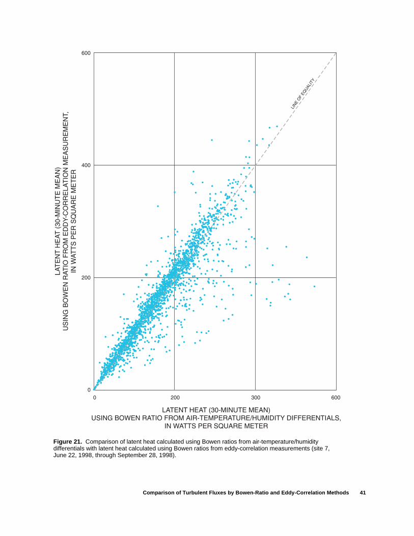
Comparison of Turbulent Fluxes by Bowen-Ratio and Eddy-Correlation Methods 41

Figure 21. Comparison of latent heat calculated using Bowen ratios from air-temperature/humidity differentials with latent heat calculated using Bowen ratios from eddy-correlation measurements (site 7, June 22, 1998, through September 28, 1998).


The data plotted in figure 21 indicate that the 30-minute latent heats calculated from both methods of determining the Bowen ratio tend to be in agreement, although the difference between the two methods is large for some intervals. For the entire period of the comparison, the mean latent heat is 164.4 W/m2 using Bowen ratios from vertical air/humidity differentials, and 162.3W/m2 using Bowen ratios from eddy-correla-tion measurements. A t-test of paired daily data indi-cates that this difference is not statistically significant at the 5 percent probability level. This lack of signifi-cant difference between the two latent-heat means indi-cates that any differences in the two methods of Bowen-ratio calculations are relatively unimportant in the calculation of latent heat.

Although the Bowen ratios determined by the two methods appear to be of similar magnitude, there is a significant difference between turbulent heat flux measured by the eddy-correlation method and the mea-sured available energy (sum of net radiation and soil/water heat flux) used to compute ET in this study. The mean of all 30-minute turbulent heat fluxes during the June 22 through September 29, 1998, period was 137.4 W/m2, and the mean of the corresponding mea-sured energy was 163.6 W/m2, or about 20 percent greater. The reason for this difference has not been determined, but has been reported in other studies (Bid-lake, Woodham, and Lopez, 1993; Goulden and others, 1997). Goulden and others (1997) noted that the energy difference became smaller with increasing friction velocity (u*), which is a function of the wind velocity profile, atmospheric stability, and the surface rough-ness that can be calculated from horizontal and vertical wind-velocity measurement (Campbell Scientific Inc., 1996). A bias in the energy difference that appears to relate to u* was also noted in comparison of turbulent flux with measured available energy at site 7.

At u* less than 0.2 meter per second (m/s), many of the 30-minute eddy-correlation-measured turbulent fluxes are considerably less than the measured avail-able energy (fig. 22). The bias seems to occur for tur-bulent flux measurements of about 50 W/m2 or less; at higher energy levels the difference between the two methods seems to be unbiased but with considerable scatter. For u* between 0.2 and 0.3 m/s, evidence of a difference between the two methods seems less but is still noticeable at low turbulent-flux levels. At higher (greater than 0.3 m/s) u*, there is little evidence of a bias in the differences, though there is considerable scatter around the line of equality.

Daily means of the turbulent fluxes and mea-sured available energy were computed and plotted in figure 23. The means contain much less scatter than the 30-minute data but generally show the same pattern as the 30-minute data plotted in figure 22. At u* values

greater than 0.3, the means from the two methods are well correlated with little or no evidence of bias. A bias is noted at lower values of u*, especially when u* is less than 0.2 m/s.

Comparison of measured energy with turbulent flux at 30-minute intervals indicates that the two energy measurements generally are in relatively good agreement in the morning and early-afternoon hours during the rising portion of the diurnal energy cycle (fig. 24). Agreement between the two measures of energy is substantially poorer in late-afternoon and evening hours, and particularly just before midnight. The reason for this pattern of differences between the two energy determinations is not definitely known, but may relate to the wind velocity effects discussed in the previous paragraph. Night-time hours generally corre-spond with low wind velocities (fig. 25), so if there is a wind effect related to the energy differences, this effect could at least partially explain the relatively large energy differences occurring around midnight.

The diurnal patterns of energy increase and decrease for measured energy and turbulent flux appear to be generally in phase with one another. This is an indication that neglecting the canopy storage in the measurement of available energy is not seriously affecting the energy budget at a 30-minute time-inter-val. If there were a noticeable effect due to canopy stor-age of energy, the measured energy (without inclusion of the canopy storage) would tend to peak earlier in the day than the peak in turbulent flux. The difference in time of peak energy would be related to the time required for the plant canopy to heat to ambient air tem-perature.

From this comparison of eddy-correlation mea-surements and Bowen-ratio station measurements, it can be concluded that the Bowen-ratio measurements using the air-temperature/humidity differential method are comparable with those calculated from eddy-corre-lation fluxes. Therefore, there is no reason to suspect that multiple energy sources or other problems are invalidating the Bowen ratios determined from the air-temperature/humidity differentials. Also, the general correspondence of daily peak energy times of both measured energy and turbulent flux tends to validate the assumption of negligible canopy heat storage in the measurement of available energy as the sum of net radi-ation and soil/water heat flux. The disagreement in total energy fluxes measured by the two methods is more problematic and is not fully understood. Although the difference seems to be related to friction velocity (u*), and is practically non-existent at values of u* greater than 0.3 m/s, the “correctness” of either method cannot be determined with the available data.

Comparison of Turbulent Fluxes by Bowen-Ratio and Eddy-Correlation Methods 43

Figure 22. Relation of 30-minute turbulent flux to measured available energy, June 22, 1998, through September 29, 1999, at site 7.


Figure 23. Relation of daily mean turbulent flux to daily mean measured available energy, June 22, 1998, through September 29, 1999, at site 7. (Daily means include only time intervals where measured available energy and turbulent flux are available. Days with less than 10 pairs of observations within the specified u* range are not plotted; u* is the frictional velocity of wind.)

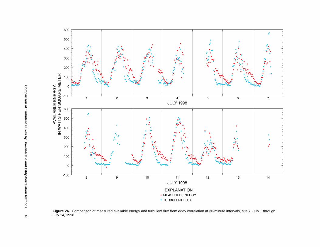
Co

mp

arison

of T

urb

ulen

t Flu

xes by B

ow

en-R

atio an

d E

dd

y-Co

rrelation

Meth

od

s45

Figure 24. Comparison of measured available energy and turbulent flux from eddy correlation at 30-minute intervals, site 7, July 1 through July 14, 1998.

46R

egio

nal E

valuatio

n o

f Evap

otran

spiratio

n in

the E

verglad

es

Figure 25. Mean wind velocity for 15-minute intervals, site 7, July 1 through July 14, 1998.

Summary and Conclusions 47

SUMMARY AND CONCLUSIONS

Nine sites were selected and instrumented for collection of data necessary for ET-determination and modeling. The Bowen-ratio energy-budget method was selected for determining ET (Bowen, 1926) because all necessary data could be obtained using automatic equipment that could operate continuously in nearly all weather conditions.

Modified Priestley-Taylor models of latent heat (ET) as a function of selected independent variables were developed at each site. These models were used to fill in periods of missing latent-heat measurements. The individual site models were combined and used to formulate regional models of ET that may be used to estimate ET in wet prairie, sawgrass or cattail marsh, and open-water portions of the natural Everglades sys-tem. The models are not applicable to forested areas or to the brackish areas adjacent to Florida Bay.

Two types of regional models were developed. One type of model uses measurements of available energy at a site, together with incoming solar energy and water depth, to estimate hourly ET. This available-energy model requires site data for net radiation, water heat storage, and soil heat flux, as well as data for incoming solar radiation and water depth. Another type of model was developed that requires only incoming solar energy, air temperature, and water-depth data to provide estimates of hourly ET. The second model thus uses data that are more readily available than the data required for the available-energy model.

For site models, standard errors were generally in the 20 to 30 percent range for 30-minute ET sums, in the 8 to 14 percent range for daily sums, and within the 3 to 7 percent range for monthly sums. Regional mod-els with available energy performed nearly as well as the site models, with standard errors that were gener-ally within the 20 to 34 percent range for 30-minute ET sums, within 10 to 16 percent range for daily sums, and within 3 to 11 percent range for monthly sums. Stan-dard errors for the regional models without available energy were larger, generally in the 30 to 90 percent range for 30-minute ET sums, within 15 to 30 percent for daily sums, and within 7 to 12 percent for the monthly sums.

Mean annual ET and ET simulated by the models generally agree within about 2 in/yr. The greatest dif-ferences between measured and modeled ET occurred for site 1, where the mean annual ET simulated by the regional model with energy was nearly 3 in. greater than the measured ET, and the ET simulated by the regional model without energy was nearly 4 in. greater than measured ET. The relatively large error at site 1

may be related to regulation of water flow through the area.

Computed ET mean annual totals for all nine sites ranged from 42.4 in/yr at site 9 to 57.4 in/yr at site 2. In general, the computed ET was greatest at the open-water sites: site 2 (57.4 in/yr) and site 3 (53.1 in/yr). Among the nearly-always-wet vegetated sites (sites 1, 4, 5, 6, and 7), ET was lower, ranging from 42.9 in/yr (site 1) to 51.2 in/yr (site 7). Excluding site 1, the range was from 46.2 to 51.2 in/yr. The ET at the two sites where the water level was below land sur-face at least several weeks each year was substantially lower than at all other sites and was 42.4 in/yr at site 9 and 43.5 in/yr at site 8.

Although the density of photosynthetically active plant leaves has been shown to relate directly to ET in some studies, it does not appear to relate directly to ET in the Everglades, based on comparison of annual ET data with leaf-area index (NDVI) data from satellite imagery. In fact, NDVI and ET seem to be inversely related in the Everglades. The greatest ET rates occurred at open-water sites where the NDVI data indi-cated the lowest leaf-area index. Among the remaining vegetated sites, there is no clear relation between ET and NDVI, though the highest ET rate corresponded to the lowest NDVI and one of the lowest ET rates corre-sponded to the highest NDVI value.

The variation in ET follows a seasonal pattern, with lowest monthly ET totals occurring in December through February, and highest ET occurring in May through August. The monthly total ET among all nine sites for the 2-year period ranged from 1.81 in. at site 1 in December 1997 to 6.84 in. at site 3 in July 1996.

Instruments for measuring heat flux by the eddy-correlation method were set up and operated together with the Bowen ratio station at site 7 for the period June 22 through September 28, 1998. Determinations of the Bowen-ratio using the air-temperature/humidity differ-ential method are comparable with those calculated from eddy-correlation fluxes. There was a considerable difference, however, in total energy measured by the two methods. The mean of all 30-minute measured tur-bulent heat fluxes from the eddy-correlation apparatus for June 22 through September 29, 1998, was 137.4 watts/m2, and the mean of the corresponding measured energy was 163.6 watts/m2, or about 20 per-cent greater. The disagreement in mean energy fluxes measured by the two methods is problematic and is not fully understood. Although the difference seems to be related to friction velocity (u*), and is practically non-existent at values of u* greater than 0.3 m/s, the “cor-rectness” of either method cannot be determined with the data available.


REFERENCES

Bidlake, W.R., Woodham, W.M., and Lopez, M.A., 1993, Evapotranspiration from areas of native vegetation in west-central Florida: U.S. Geological Survey Open-File Report 93-415, 35 p.

Bowen, I.S., 1926, The ratio of heat losses by conduction and by evaporation from any water surface: Physical Review, 2nd series, v. 27, no. 6, p. 779-787.

Brutsaert, Wilfried, 1991, Evaporation into the atmosphere: Kluwer Academic Publishers, Netherlands, 299 p.

Campbell Scientific Inc., 1990, TCAV averaging soil ther-mocouple probe instruction manual: Logan, Utah, 2 p.

Campbell Scientific Inc., 1996, CSAT3 three dimensional sonic anemometer instruction manual: Logan, Utah, 57 p.

Carter, V., Reel, J.T., Rybicki, N.B., Ruhl, H.A., Gammon, P.T., and Lee, J.K., 1999, Vegetative resistance to flow in south Florida: Summary of vegetation sampling at sites NESRS3 and P33, Shark River Slough, November, 1996: U.S. Geological Survey Open-File Report 99-218, 90 p.

Davies, J.A., and Allen, C.D., 1973, Equilibrium, potential and actual evaporation from cropped surfaces in south-ern Ontario: Journal of Applied Meteorology, v. 12, p. 649-657.

De Bruin, H.A.R., 1983, A model for the Priestley-Taylor parameter α: Journal of Climate and Applied Meteorol-ogy, v. 22, p. 572-578.

Douglas, M.S., 1947, The Everglades: River of grass: Mockingbird Books, St. Simons Island, Ga., 1974, p. 16.

Fritschen, L.J., and Gay, L.W., 1979, Environmental instru-mentation: Springer-Verlag, New York, 209 p.

Goulden, M.L., Daube, B.C., Fan, Song-Miao, Sutton, D.J., Bazzaz, A., Munger, J.W., and Wofsy, S.C., 1997, Phys-iological responses of a black spruce forest to weather: Journal of Geophysical Research, v. 102, no. D24, p. 28,987-28,996.

Knowles, Leel, Jr., 1996, Estimation of evapotranspiration in the Rainbow Springs and Silver Springs Basins in north-central Florida: U.S. Geological Survey Water-Resources Investigations Report 96-4024, p. 24.

Lodge, T.E., 1994, The Everglades handbook: Understand-ing the ecosystem: St. Lucie Press, Delray Beach, Fla., 228 p.

Monteith, J.L., 1965, Evaporation and environment, in The state and movement of water in living organisms, Sym-posium of the Society of Experimental Biology: San Diego, California (G.E. Fogg, ed.), Academic Press, New York, p. 205-234.

McPherson, B.F., Higer, A.L., Gerould, Sarah, and Kantrow-itz, I.H., 1995, South Florida ecosystem program of the U.S. Geological Survey: Fact Sheet 134-95, 4 p.

Ohmura, Atsumu, 1982, Objective criteria for rejecting data for Bowen ratio flux calculations: Journal of Applied Meteorology, v. 21, p. 595-598.

Pereira, A.R., and Villa Nova, N.A., 1992, Analysis of the Priestley-Taylor parameter: Agricultural and Forest Meteorology, v. 61, p. 1-9.

Priestley, C.H.B., and Taylor, R.J., 1972, On the assessment of surface heat flux and evaporation using large-scale parameters: Monthly Weather Review, v. 100, p. 81-92.

Schotanus, P., Nieuwstadt, F.T.M., and De Bruin, H.A.R., 1983, Temperature measurement with a sonic anemom-eter and its application to heat and moisture fluxes: Boundary-Layer Meteorology, v. 26, p. 81-93.

Stannard, D.I., 1993, Comparison of Penman-Monteith, Shuttleworth-Wallace, and modified Priestley-Taylor evapotranspiration models for wildlife vegetation in semiarid rangeland: Water Resources Research, v. 29, no. 5, p. 1379-1392.

Sumner, D.M., 1996, Evapotranspiration from successional vegetation in a deforested area of the Lake Wales Ridge, Florida: U.S. Geological Survey Water-Resources Investigations Report 96-4244, 38 p.

Tanner, B.D., and Greene, J.P., 1989, Measurement of sensi-ble heat and water vapor fluxes using eddy correlation methods: Final report prepared for U.S. Army Dugway Proving Grounds, Dugway, Utah, 17 p.

Tanner, C.B., and Thurtell, G.W., 1969, Anemoclinometer measurements of Reynolds stress and heat transport in the atmospheric surface layer: Final Report prepared for United States Army Electronics Command, Atmo-spheric Sciences Laboratory, Fort Huachuca, Arizona, 10 p.

Webb, E.K., Pearman, G.I., and Leuning, R., 1980, Correc-tion of flux measurements for density effects due to heat and water vapor transfer: Quarterly Journal of the Royal Meteorological Society, v. 106, p. 85-100.

d:\usgs reports\authors\german\et finals\et eps finals\et4217

Documents