Computational Mechanics manuscript No.(will be inserted by the editor)

Dynamic and fluid–structure interaction simulations of bioprostheticheart valves using parametric design with T-splines and Fung-typematerial models

Ming-Chen Hsu · David Kamensky · Fei Xu · Josef Kiendl ·Chenglong Wang · Michael C.H. Wu · Joshua Mineroff ·Alessandro Reali · Yuri Bazilevs · Michael S. Sacks

The final publication is available at Springer via http://dx.doi.org/10.1007/s00466-015-1166-x

Abstract This paper builds on a recently developed immer-sogeometric fluid–structure interaction (FSI) methodologyfor bioprosthetic heart valve (BHV) modeling and simula-tion. It enhances the proposed framework in the areas ofgeometry design and constitutive modeling. With these en-hancements, BHV FSI simulations may be performed withgreater levels of automation, robustness and physical real-ism. In addition, the paper presents a comparison betweenFSI analysis and standalone structural dynamics simulationdriven by prescribed transvalvular pressure, the latter beinga more common modeling choice for this class of prob-lems. The FSI computation achieved better physiologicalrealism in predicting the valve leaflet deformation than itsstandalone structural dynamics counterpart.

Keywords Fluid–structure interaction · Bioprosthetic heartvalve · Isogeometric analysis · Immersogeometric analysis ·Arbitrary Lagrangian–Eulerian · NURBS and T-splines ·Kirchhoff–Love shell · Fung-type hyperelastic model

M.-C. Hsu (�) · F. Xu · C. Wang ·M. C. H. Wu · J. Mineroff

Department of Mechanical Engineering, Iowa State University, 2025Black Engineering, Ames, IA 50011, USAE-mail: jmchsu@iastate.edu

D. Kamensky ·M. S. SacksCenter for Cardiovascular Simulation, Institute for Computational En-gineering and Sciences, The University of Texas at Austin, 201 East24th St, Stop C0200, Austin, TX 78712, USA

J. Kiendl · A. RealiDepartment of Civil Engineering and Architecture, University of Pavia,via Ferrata 3, 27100 Pavia, Italy

Y. BazilevsDepartment of Structural Engineering, University of California, SanDiego, 9500 Gilman Drive, Mail Code 0085, La Jolla, CA 92093, USA

1 Introduction

Heart valves serve to ensure unidirectional flow of bloodthrough the circulatory systems of humans and many ani-mals. Heart valves consist of thin, flexible leaflets that openand close passively, in response to blood flow and the move-ments of the attached cardiac structures. Primarily in aorticheart valves, the leaflets may become diseased and, in somecases, valves must be replaced by prostheses. Hundreds ofthousands of such devices are implanted in patients everyyear [1, 2].

The most popular class of prostheses are bioprostheticheart valves (BHVs). BHVs imitate the structure of the na-tive valves, consisting of flexible leaflets fabricated fromchemically-treated soft tissues. BHVs do not induce blooddamage that can occur due to prostheses composed of rigidmechanical parts [2–4]. However, BHVs are less durablethan their mechanical counterparts and require replacement,typically after 10–15 years, due to calcification and struc-tural damage [5]. In spite of this long-standing problem,BHV material technologies have not changed since their in-troduction more than 30 years ago.

Improved durability remains an important clinical goaland represents a unique cardiovascular engineering chal-lenge, resulting from the extreme valvular mechanical de-mands. Yet, current BHV assessment relies exclusively ondevice-level evaluations, which are confounded by simulta-neous and highly coupled biomaterial mechanical fatigue,valve design, hemodynamics, and calcification. Thus, de-spite decades of clinical BHV usage and growing pop-ularity, there exists no acceptable method for simulatingBHV durability in any design context. There is thus a pro-found need for the development of novel simulation tech-nologies that combine state-of-the-art fluid–structure inter-action (FSI) analysis with novel constitutive models of BHV

2 Ming-Chen Hsu et al.

biomaterial responses, to simulate long-term cyclic load-ing [6, 7].

Computational modeling of continuum mechanics hasproven tremendously beneficial to the design process ofmany other products, but BHVs present unique challengesfor computational analysis, and cannot yet be convenientlysimulated using “off-the-shelf” software. The effect of hy-drostatic forcing on a closed BHV may be modeled as aprescribed pressure load and simulated using standard FEM(see, e.g., [8–10]), but such models cannot capture the tran-sient response of an opening valve or the so-called “waterhammer effect” in a closing valve. Both of these phenom-ena likely contribute to long-term structural fatigue, but nei-ther can be modeled without accounting for the surroundinghemodynamics. A complete mechanical model of a BHVmust therefore include FSI.

In [11, 12], we developed a new numerical method that,in the tradition of immersed boundary methods [13–16], al-lows the structure discretization to move independently ofthe background fluid mesh. In particular, we focused on di-rectly capturing design geometries in the unfitted analysismesh and identified our technique with the concept of im-mersogeometric analysis. The methods that we developedin [11, 12] made beneficial use of isogeometric analysis(IGA) [17,18] to discretize both the structural and fluid me-chanics subproblems involved in the FSI analysis of BHVs.In this paper, we further advance our immersogeometric FSImethodology for BHVs by focusing on automating the IGAmodel design and improving constitutive modeling of thechemically-treated tissues forming the BHV leaflets.

Despite recent progress, several challenges remain in theeffective use of IGA to improve the engineering design pro-cess. A major difficulty toward this end remains automatic(or semi-automatic) construction of analysis-suitable IGAmodels. In many cases, intimate familiarity with computer-aided design (CAD) technology and advanced programmingskills are required to create high-quality IGA geometries andmeshes. In a recent work [19] the authors introduced an in-teractive geometry modeling and parametric design platformthat streamlines the engineering design process by hidingthe complex CAD functions in the background through gen-erative algorithms, and letting the user control the designthrough key parameters. In the present work, we apply thisdesign-through-analysis framework to BHV analysis.

We further enhance the realism of the BHV FSI by ex-tending the isogeometric rotation-free Kirchhoff–Love thinshell formulation [20, 21] used in the prior work to includethe soft-tissue constitutive modeling framework developedin [22]. An important feature of the framework in [22] isthat it can accommodate arbitrary hyperelastic constitutivemodels, which adds a great deal of flexibility to the BHVFSI methodology developed in this work.

The remainder of this paper is structured as follows.Section 2 describes our BHV FSI modeling framework andmethods. In Section 3, we construct a discrete model of aBHV immersed in the lumen of a flexible artery and applythe methodology of Section 2 to perform a BHV FSI sim-ulation. We compare the FSI results with the results of astandalone structural dynamics BHV simulation driven byprescribed transvalvular pressure, considered to be “state-of-the-art” in the biomechanics community [9]. Section 4draws conclusions.

2 BHV FSI modeling framework and methods

In this section we present the main constituents of the re-cently developed FSI modeling framework for heart valves,focusing on the novel contribution of the present article. Webegin by providing a discussion of the recently developedparametric design-through-analysis platform for IGA [19]and its use in the modeling of heart valve geometry. We thensummarize the shell formulation proposed in [22], whichwe use to incorporate incompressible Fung-type hyperelas-tic material behavior into our BHV simulations. We thenprovide an overview of the immersogeometric FSI [11] pro-cedures employed to simulate this challenging class of prob-lems.

2.1 Parametric modeling of heart valve geometry

In [19], an interactive geometry modeling and parametricdesign platform was proposed to help design engineers andanalysts make effective use of IGA. Several Rhinoceros(Rhino) [23] “plug-ins”, with a user-friendly interface, werecreated to take input design parameters, generate parame-terized surface and/or volumetric models, perform compu-tations, and visualize the solution fields, all within the sameCAD program. An important aspect of the proposed plat-form is the use of generative algorithms for IGA model cre-ation and visualization. In this work, we make use of the de-veloped platform to automate the geometry design of BHVmodels for use in FSI analysis.

The developments in [19] were based on Rhino CADsoftware, which gives designers a variety of functions thatare required to build complex, multi-patch NURBS sur-faces [25]. Recently, additional functionality was added inRhino to create and manipulate T-spline surfaces [24, 26].This is an important enhancement that allows one to moveaway from a fairly restrictive NURBS-patch-based geome-try design to a completely unstructured, watertight surfacedefinition respecting all the constraints imposed by analy-sis [27, 28]. Rhino also features a graphic programming in-terface called Grasshopper [29] suitable for parametric de-sign, and utilizes open-source software development kits

Title Suppressed Due to Excessive Length 3

Fig. 1: The trileaflet T-spline BHV model in Rhino. TheT-spline surfaces were generated using the in-house para-metric modeling platform (see Fig. 2) and the Autodesk T-Splines Plug-in for Rhino [24].

(SDK) [30] for plug-in development. Furthermore, Rhino isrelatively transparent as compared to other CAD software inthat it provides the user with the ability to interact with thesystem through the plug-in commands. All of these featuresare well aligned with the needs of analysis-suitable geome-try design for BHVs, and are employed in the present work.

Fig. 1 shows a snapshot of the Rhino CAD modelingsoftware interface, with the T-spline BHV model used inthe computations of the present paper. This BHV leafletgeometry is based on a 23-mm design by Edwards Life-sciences [8, 31]. The NURBS version of this model was an-alyzed earlier in [11, 12]. In the present case, the leaflets ofthe BHV are modeled using three cubic T-spline surfaces, asshown in Fig. 1. The use of unstructured T-splines enableslocal refinement and coarsening [32] and avoids the small,degenerated NURBS elements near the commissure pointsused in [11, 12]. To improve the realism of the simulation,we include the metal stent in the BHV model. Although thiscomplicates the geometry, it presents no difficulty for thedesign platform employed in this work to generate a singlewatertight surface.

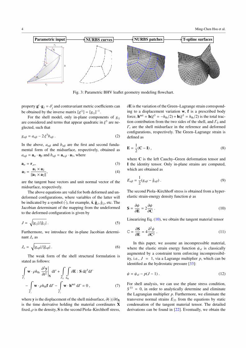
Using Grasshopper as a visual programming tool, theprogram that creates an analysis-suitable geometry design iswritten in terms of “components” with pre-defined or user-defined functionalities, and “wire connections” between thecomponents that serve as conduits of input and outputdata. As a result, using an intuitive arrangement of compo-nents and connections one can rapidly generate an analysismodel and establish parametric control over the design. AGrasshopper program for the geometry design of the BHVleaflet employed in this work is shown in Fig. 2. The vi-sual program executes the following geometry construction

Fig. 2: The Grasshopper program for parametric BHV leafletgeometry modeling. (This figure is intended for zoomedviewing.) The major geometry construction steps are shownin Fig. 3.

steps (see Fig. 3 for a visual illustration): Parametric inputis used to construct NURBS curves, which are the bound-ing curves for the NURBS surface patches that define thevalve leaflet geometry. The resulting multi-patch NURBSgeometry is then re-parameterized to create a single T-splinesurface geometry. Following this workflow, new analysis-suitable geometries can be easily and efficiently generatedusing different sets of input design parameters.

Remark 1 Note that the stent can be generated using thesame parametric geometry modeling approach. It is not in-cluded in Figs. 2 and 3 for the sake of clarity and simplicityof presentation.

2.2 Shell structural formulation

The leaflet structure is modeled as a hyperelastic thin shellwith isogeometric discretization as presented in Kiendl etal. [22]. Due to the Kirchhoff–Love hypothesis of normalcross sections, a point x in the shell continuum can be de-scribed by a point r on the midsurface and a normal vectora3 to the midsurface as

x(ξ1, ξ2, ξ3) = r(ξ1, ξ2) + ξ3 a3(ξ1, ξ2) , (1)

where ξ1, ξ2 are the surface coordinates, ξ3 ∈ [−hth/2, hth/2]is the thickness coordinate, and hth is the shell thickness.Covariant base vectors and metric coefficients are definedby gi = x,i and gi j = gi · g j, respectively, where the no-tation (·),i = ∂(·)/∂ξi is used for partial derivatives. Further-more, we adopt the convention that Latin indices take on val-ues {1, 2, 3} while Greek indices take on values {1, 2}. Con-travariant base vectors gi are defined by the Kronecker delta

4 Ming-Chen Hsu et al.

Parametric input NURBS curves NURBS patches T-spline surfaces

h

r1

r2

θ1

θ2

θ3

Fig. 3: Parametric BHV leaflet geometry modeling flowchart.

property gi ·g j = δij and contravariant metric coefficients can

be obtained by the inverse matrix [gi j] = [gi j]−1.For the shell model, only in-plane components of gi j

are considered and terms that appear quadratic in ξ3 are ne-glected, such that

gαβ = aαβ − 2 ξ3bαβ . (2)

In the above, aαβ and bαβ are the first and second funda-mental form of the midsurface, respectively, obtained asaαβ = aα · aβ and bαβ = aα,β · a3, where

aα = r,α, (3)

a3 =a1 × a2

||a1 × a2||, (4)

are the tangent base vectors and unit normal vector of themidsurface, respectively.

The above equations are valid for both deformed and un-deformed configurations, where variables of the latter willbe indicated by a symbol ˚(·), for example, x, g,i, gi j, etc. TheJacobian determinant of the mapping from the undeformedto the deformed configuration is given by

J =

√|gi j|/|gi j| . (5)

Furthermore, we introduce the in-plane Jacobian determi-nant Jo as

Jo =

√|gαβ|/|gαβ| . (6)

The weak form of the shell structural formulation isstated as follows:∫Γt

w · ρhth∂2y∂t2

∣∣∣∣∣∣X

dΓ +

∫Γ0

∫hth

δE : S dξ3dΓ

−

∫Γt

w · ρhthf dΓ −∫Γt

w · hnet dΓ = 0 , (7)

where y is the displacement of the shell midsurface, ∂(·)/∂t|Xis the time derivative holding the material coordinates Xfixed, ρ is the density, S is the second Piola–Kirchhoff stress,

δE is the variation of the Green–Lagrange strain correspond-ing to a displacement variation w, f is a prescribed bodyforce, hnet = h(ξ3 = −hth/2) + h(ξ3 = hth/2) is the total trac-tion contribution from the two sides of the shell, and Γ0 andΓt are the shell midsurface in the reference and deformedconfigurations, respectively. The Green–Lagrange strain isdefined as

E =12

(C − I) , (8)

where C is the left Cauchy–Green deformation tensor andI the identity tensor. Only in-plane strains are computed,which are obtained as

Eαβ =12

(gαβ − gαβ) . (9)

The second Piola–Kirchhoff stress is obtained from a hyper-elastic strain-energy density function ψ as

S =∂ψ

∂E= 2

∂ψ

∂C. (10)

Linearizing Eq. (10), we obtain the tangent material tensor

C =∂S∂E

= 4∂2ψ

∂C2 . (11)

In this paper, we assume an incompressible material,where the elastic strain energy function ψel is classicallyaugmented by a constraint term enforcing incompressibil-ity, i.e., J = 1, via a Lagrange multiplier p, which can beidentified as the hydrostatic pressure [33]:

ψ = ψel − p(J − 1) . (12)

For shell analysis, we can use the plane stress condition,S 33 = 0, in order to analytically determine and eliminatethe Lagrangian multiplier p. Furthermore, we eliminate thetransverse normal strains E33 from the equations by staticcondensation of the tangent material tensor. The detailedderivations can be found in [22]. Eventually, we obtain the

Title Suppressed Due to Excessive Length 5

following equations for the shell’s stress and material tan-gent tensors:

S αβ = 2∂ψel

∂Cαβ− 2

∂ψel

∂C33J−2

o gαβ , (13)

Cαβγδ = 4∂2ψel

∂Cαβ∂Cγδ+ 4

∂2ψel

∂C233

J−4o gαβgγδ

− 4∂2ψel

∂C33∂CαβJ−2

o gγδ − 4∂2ψel

∂C33∂CγδJ−2

o gαβ

+ 2∂ψel

∂C33J−2

o (2gαβgγδ + gαγgβδ + gαδgβγ) . (14)

With Eqs. (13) and (14), arbitrary 3D constitutive mod-els can be used for shell analysis directly. Given the firstand second derivatives of the elastic strain energy function,the incompressibility and plane stress constraints, as wellas static condensation of the thickness stretch, are all in-cluded by the additional terms in Eqs. (13) and (14). Re-calling Eq. (2), it can be seen that the whole formulationcan be completely described in terms of the first and secondfundamental forms of the shell midsurface, and using onlydisplacement degrees of freedom.

To discretize the shell equations we use IGA based on T-splines, which have the necessary continuity properties. Thedetails of constructing smooth T-spline basis functions canbe hidden from the analysis code through the use of Bezierextraction [34]. The extraction operators specifying the re-lationship between the T-spline basis functions and Bern-stein polynomial basis on each Bezier element can be gen-erated automatically by the Autodesk T-Splines Plug-in forRhino [24,26]. The mesh of Bezier elements for our T-splineBHV model is shown in Fig. 4.

2.3 Immersogeometric FSI

In this section we summarize the main constituents of ourframework for immersogeometric FSI, as it applies to thesimulation of BHVs. For mathematical and implementationdetails the reader is referred to [11, 12, 35]. Our immerso-geometric approach to BHV FSI analysis combines the fol-lowing computational technologies into a single framework:

• The blood flow in a deforming artery is governed by theNavier–Stokes equations of incompressible flows posedon a moving domain. The domain motion is handled us-ing the Arbitrary Lagrangian–Eulerian (ALE) formula-tion [36, 37], which is a widely used approach for vas-cular blood flow applications [38–44]. For an overviewof the ALE method in cardiovascular fluid mechan-ics, see [45, 46]. These two references also include anoverview of the space–time approach to moving do-mains [47–51], which has also been applied to a goodnumber of cardiovascular fluid mechanics computations,with the most recent ones reported in [52–55].

Fig. 4: The Bezier elements defining the T-spline surfaceused in the shell analysis. The clamped boundary conditionis applied to the leaflet attachment edge by fixing two rowsof T-spline control points highlighted in the figure. (Thepoints in the second row away from the edge are also calledtangency handles.)

• The blood flow domain follows the motion of the de-formable artery wall, which is governed by equationsof large-deformation elastodynamics written in the La-grangian frame [56]. In the present work, the discretiza-tion between blood flow and artery wall is assumed tobe conforming, and is handled using a monolithic FSIformulation described in detail in [57].

• The discretization of the Navier–Stokes equations makesuse of a combination of NURBS-based IGA and ALE–VMS [58–60]. The ALE–VMS formulation may be in-terpreted both as a stabilized method [47, 61, 62] andas a large-eddy simulation (LES) turbulence model [47,61–67]. The discretization of the solid arterial wall alsomakes use of trivariate NURBS-based IGA.

• BHV leaflets are modeled as rotation-free hyperelasticKirchhoff–Love shell structures (see [22] and the previ-ous section) and discretized using T-splines. In the FSIframework, they are immersed into a moving blood-flowdomain. The immersed FSI problem is formulated usingan augmented Lagrangian approach for FSI, which wasoriginally proposed in [68] to handle boundary-fittedmesh computations with nonmatching fluid–structure in-terface discretizations. It was found in [11] that the aug-mented Lagrangian framework naturally extends to non-boundary-fitted (i.e., immersed) FSI problems, but withthe following modifications. The tangential componentof the Lagrange multiplier λλλ is formally eliminated from

6 Ming-Chen Hsu et al.

the formulation, resulting in weak enforcement of no-slip conditions at the fluid–structure interface [68]. Thenormal component of the Lagrange multiplier λ = λλλ · nis retained in the formulation in order to achieve bettersatisfaction of no-penetration boundary conditions at thefluid–structure interface.

• The Lagrange multiplier field is discretized by collocat-ing the normal-direction kinematic constraint at quadra-ture points of the fluid–structure interface and involvesadding a scalar unknown at each one of these quadra-ture points. In the evaluations of integrals involved inthe augmented Lagrangian formulation these multiplierunknowns are treated as point values of a function de-fined at the fluid–structure interface. In the computa-tions, λ is treated in a semi-implicit fashion. Namely, thepenalty terms in the augmented Lagrangian formulationare treated implicitly, while the resulting penalty force isused to update λ explicitly in each time step.

• Contact between BHV leaflets is an essential featureof a functioning heart valve. During the closing stage,the BHV leaflets contact one another to prevent leak-age of blood back into the left ventricle. In the contextof immersed FSI approaches, pre-existing contact meth-ods and algorithms (see, e.g., [69, 70]) may be incorpo-rated directly into the framework without any modifi-cation or concern for fluid-mechanics mesh quality. Inthe present work, we adopt a penalty-based approach forsliding contact and impose contact conditions at quadra-ture points of the shell structure. The use of smooth basisfunctions improves the performance of contact betweenvalve leaflets (see, e.g., [71]).

• BHV simulations involve flow reversal at outflowboundaries, which, unless handled appropriately, oftenleads to divergence in the simulations. In order to pre-clude this backflow divergence, an outflow stabilizationmethod originally proposed in [72] and further studiedin [73] is incorporated into the FSI framework.

• We use a novel semi-implicit time integration procedure:1. Solve implicitly for the fluid, solid structure, mesh

displacement, and shell structure unknowns, holdingthe Lagrange multiplier λ fixed at its current value.Note that the fluid and shell structure are coupled inthis subproblem due to the presence of penalty termsin the augmented Lagrangian framework. The im-plicit system is formulated based on the Generalized-α technique [57, 74, 75].

2. Update the Lagrange multiplier λ by adding thenormal component of penalty forces coming fromthe fluid and structure solutions from Stage 1. Inthis work, we stabilize this update following refer-ence [35], scaling the updated multiplier by 1/(1+r),where r is a nonnegative, dimensionless constant.

As detailed in [11], the above semi-implicit solutionprocedure is algorithmically equivalent to fully implicitintegration of a “stiff” differential-equation system ap-proximating the constrained differential–algebraic sys-tem. The stiffness increases as the time step shrinks, butthe conditioning of Stage 1 remains unaffected. A recentreference [35] showed that a stiff differential equationsystem is energetically stable in a simplified model prob-lem, even when r = 0. To solve the nonlinear coupledproblem in Stage 1, a combination of the quasi-directand block-iterative FSI coupling strategies is adopted(see [76–79]). The complete algorithm is given in [12].

Remark 2 Our framework falls under the umbrella of theFluid–Solid Interface-Tracking/Interface-Capturing Tech-nique (FSITICT) [80]. The FSITICT targets FSI problemswhere interfaces that are possible to track are tracked, andthose too challenging to track are captured. The FSITICTwas introduced as an FSI version of the Mixed Interface-Tracking/Interface-Capturing Technique (MITICT) [81].The MITICT was successfully tested in 2D computationswith solid circles and free surfaces [82, 83], and in 3D com-putation of ship hydrodynamics [84]. The FSITICT was re-cently employed in [85] to compute several 2D FSI bench-mark problems.

Remark 3 On the fluid mechanics domain interior, the meshmotion is obtained by solving a sequence of linear elasto-static problems subject to the displacement boundary con-ditions coming from the artery wall. In the formulationof the elastostatics problems, the Jacobian stiffening tech-nique is employed to protect the boundary-layer mesh qual-ity [86–89].

Remark 4 It was shown in [90–93] that imposing Dirich-let boundary conditions weakly allows the flow to slip onthe solid surface, which, in turn, relaxes the boundary-layer resolution requirements to achieve the desired so-lution accuracy. In the non-boundary-fitted FSI, the fluidmesh is arbitrarily cut by the structural boundary, leavinga boundary-layer discretization of inferior quality comparedto the boundary-fitted case. As a result, weakly enforced no-slip conditions, which naturally arise in the augmented La-grangian framework, simultaneously lead to imposition ofthe physical kinematic constraints at the fluid–structure in-terface, and, as an added benefit, enhance the accuracy ofthe fluid mechanics solution near the interface.

Remark 5 During the closing stage, the BHV leaflets con-tact one another to block reversed flow to the left ventricle.As a result, the contact formulation employed must be suchthat no gap is allowed between the leaflets. This, in turn,leads to a topology change in the problem, and presentsone of the main reasons in the literature for developing

Title Suppressed Due to Excessive Length 7

non-boundary-fitted FSI techniques for the present applica-tion. Reference [53] recently demonstrated how space–timeFEM, in combination with appropriately defined master–slave relationships between the mesh nodes in the fluid me-chanics domain, can deliver solutions for cases with topol-ogy change without resorting to immersed techniques. Thespace–time with topology change (ST-TC) technique wassuccessfully applied in the CFD simulation of an artificialheart valve with prescribed leaflet motion in [55].

3 BHV simulations

We compute pressure-driven structural dynamics and FSIof the BHV shown in Fig. 4. In particular, we consider aBHV replacing an aortic heart valve, which regulates flowbetween the left ventricle of the heart and the aorta. Duringsystole, when the heart contracts, the valve permits ejectionof oxygenated blood from the left ventricle into the aorta,and, during diastole, as the heart relaxes, a correctly func-tioning aortic valve prohibits regurgitation of blood backinto the expanding ventricle. Sections 3.1 and 3.2 describethe modeling of the BHV and the surrounding artery andlumen, while Section 3.3 focuses on the comparison of thestructural dynamics and FSI simulation results.

3.1 BHV constitutive model and boundary conditions

Biological tissues are favored in the construction of BHVsdue to their unique mechanical properties. The most impor-tant of these is that they remain compliant at low strainsbut stiffen dramatically when stretched, allowing for ease ofmotion without sacrificing durability. The underlying struc-tural mechanism is the presence of collagen fibers whichare highly undulated in unloaded tissue. These fibers pro-vide only small bending stiffnesses in unloaded tissue, buttheir relatively larger tensile stiffness can be recruited whenthey are straightened under strain. One of the earliest andmost widely used models uses an exponential function ofstrain to describe the stiffening of tissues under tensile load-ing [94–96]. It is widely referred to as Fung models. Forsmaller bending strains, such as those in an open aortic BHVduring systole, the dominant contribution to material stiff-ness is the extracellular matrix (ECM), which supports thenetwork of collagen fibers. Reference [97] advocates model-ing ECM as an incompressible neo-Hookean contribution tothe strain-energy density functional. In this work, we com-bine an isotropic Fung model of collagen fiber stiffness witha neo-Hookean model of cross-linked ground matrix stiff-ness to obtain the following strain-energy density functional:

ψel =c0

2(I1 − 3) +

c1

2

(ec2(I1−3)2

− 1)

, (15)

where c0, c1, and c2 are material parameters. This modelis combined with the incompressibility constraint as inEq. (12). Note that while Eq. (15) is a simplified isotropicapproximation to true anisotropic leaflet behaviors, it cap-tures the important exponential nature of the BHV soft tis-sue behavior.

The mass density of the leaflets is set to 1.0 g/cm3. Thematerial parameters are set to c0 = 1.0 × 106 dyn/cm2,c1 = 2.0 × 105 dyn/cm2, and c2 = 100. The values of c1 andc2 provide tensile stiffnesses that are generally comparableto those of the more complicated pericardial BHV leafletmodel considered in [8]. The ECM modulus c0 is selectedto provide a small-strain bending stiffness similar to that ofglutaraldehyde-treated bovine pericardium, as measured bythe three-point bending tests reported in [98]. The hypere-lastic thin shell analysis framework of Section 2.2 requiresthe following derivatives of the strain energy functional inEqs. (13) and (14):

∂ψel

∂Ci j=

12

(c0 + 2c1c2(I1 − 3)ec2(I1−3)2)

gi j , (16)

∂2ψel

∂Ci j∂Ckl= c1c2ec2(I1−3)2 (

1 + 2c2(I1 − 3)2)

gi jgkl . (17)

The BHV model employs the T-spline geometry con-structed in Section 2.1. The T-spline mesh comprises 484and 882 Bezier elements for each leaflet and the stent, re-spectively, and a total of 2,301 T-spline control points. Thestent is assumed rigid, and leaflet control points highlightedin Fig. 4 are restrained from moving. This clamps the at-tached edges of the leaflets to the rigid stent. (The stent is,for all practical purposes, rigid since it is supported by ametal frame, which is orders of magnitude stiffer than thesoft tissue of the BHV leaflets.) The leaflet thickness is setto a uniform value of 0.0386 cm.

Remark 6 The use of pinned rather than clamped boundaryconditions is common in the structural analysis of BHVsreported previously [9, 31, 99–101]. However, the leafletsare, in fact, physically clamped at the attachment edge inmost stented BHVs (see, e.g., [102, 103]). As shown laterin the paper, using clamped boundary conditions, the com-puted fully-open configuration of the leaflets is closer to theexperimental measurements of pericardial BHV deforma-tions [104–106] than results computed using pinned bound-ary conditions in [11, 12].

To elucidate the physical significance of the Fung-typematerial model given by Eq. (15) in the context of BHV de-sign, we compare its behavior to that of the classical St.Venant–Kirchhoff material, which assumes a linear stress–strain relationship and can not capture the exponential stiff-ening behavior of soft tissues. Fig. 5 compares MIPE1 in

1 Maximum in-plane principal Green-Lagrange strain, the largesteigenvalue of E.

8 Ming-Chen Hsu et al.

Fig. 5: Comparison between different isotropic materialmodels. The valve is loaded with a spatially-uniform pres-sure of 100 mmHg. The maximum values of MIPE are 0.490and 0.319 for St. Venant–Kirchhoff and Fung-type cases, re-spectively.

pressure-loaded, fully-closed configurations of a valve mod-eled using the Fung-type material described above and avalve of the same geometry modeled using an isotropicSt. Venant–Kirchhoff material with Young’s modulus E =

1.1 × 107 dyn/cm2 and Poisson’s ratio ν = 0.495. The valueof E is chosen such that the overall deformations are visu-ally similar. The results show that the peak strain in the St.Venant–Kirchhoff material is much larger. The exponentialterm in the Fung-type energy functional ensures that regionsof concentrated strain are energetically unfavorable, whichhas the effect of distributing strains more evenly through theleaflets.

3.2 Model of the artery and lumen

We model the artery as a 16 cm long elastic cylindrical tubewith a three-lobed dilation near the BHV, as shown in Fig. 6.This dilation corresponds to the aortic sinus, which is knownto play an important role in heart valve dynamics [107]. Thecylindrical portion of the artery has an inside diameter of 2.6cm and a wall thickness of 0.15 cm. The outflow boundaryis 11 cm downstream of the valve, located at the right end ofthe channel, based on the orientation of Fig. 6. The inflowis located 5 cm upstream, at the left end of the channel. Thedesignations of inflow and outflow are based on the prevail-ing flow direction during systole. In general, fluid may movein both directions and there is typically some regurgitationduring diastole.

The arterial geometry is constructed using trivariatequadratic NURBS, allowing us to represent the circular por-tions exactly. We use a multi-patch design to avoid havinga singularity at the center of the cylindrical sections (seeFig. 7). Basis functions are made C0-continuous by repeatedknot insertion at the fluid–solid interface, to capture the con-tinuous but non-smooth velocity field across this jump inmaterial type. The solid subdomain corresponds to the elas-

tic aortic wall, while the fluid subdomain is the enclosedlumen. The mesh of the lumen and aortic wall consists of102,960 and 12,480 elements, respectively. Mesh refinementis focused near the valve and sinus, as shown in Fig. 6. Fig. 7shows that the mesh is clustered toward the wall to bettercapture the boundary layer solution in those regions.

The arterial wall is modeled as a neo-Hookean mate-rial with dilatational penalty (see, e.g. [57, 108]), where theshear and bulk modulii of the model are selected to producea Young’s modulus of 1.0 × 107 dyn/cm2 and Poisson’s ra-tio of 0.45 in the small-strain limit. The density of the arte-rial wall is 1.0 g/cm3. Mass-proportional damping is addedto model the interaction of the artery with surrounding tis-sue and interstitial fluid, with the damping coefficient set to1.0 × 104 s−1. The fluid density and viscosity in the lumenare set to ρ1 = 1.0 g/cm3 and µ = 3.0 × 10−2 g/(cm s), re-spectively, which model the physical properties of humanblood [109, 110].

The inlet and outlet of the artery are free to slide in theircut planes, but constrained not to move in the orthogonaldirection (see [42] for details). The outer wall of the arteryhas a zero-traction boundary condition. The BHV stent issurgically sutured to the aortic annulus at the suture ring.Since the stent is assumed not to move in this work, we applyhomogeneous Dirichlet conditions to any control point ofthe solid portion of the artery mesh whose correspondingbasis function’s support intersects the stationary stent. Fig. 8shows geometrically how the base ring intersects with thesolid wall. The size of the ring can influence the potentialspace for blood flow and thus is important to be included inthe FSI simulation. The stent also properly seals the gap inthe fluid domain between the attached edges of the leafletsand the aortic wall.

3.3 Computations and results

This section sets up and compares the results of simulationsof BHV function that are based on standalone structural dy-namics and FSI.

3.3.1 Details of the structural dynamics simulation

In the structural dynamics computation, we model thetransvalvular pressure (i.e., pressure difference between leftventricle and aorta) with the traction −P(t)n, where P(t) isthe pressure difference at time t shown in Fig. 9, and n isthe surface normal pointing from the aortic to the ventricularside of each leaflet. The transvalvular pressure signal is peri-odic with a period 0.86 s. As in the computations of [11,31],we use damping to model the viscous and inertial resistanceof the surrounding fluid. We apply this damping as a trac-tion −cdu, where u is the velocity of the shell midsurfaceand cd = 80 g/(cm2 s). This value of cd ensures that the

Title Suppressed Due to Excessive Length 9

Fig. 6: A view of the arterial wall and lumen into which the valve is immersed.

Fig. 7: Cross-sections of the fluid and solid meshes, takenfrom the cylindrical portion and the sinus.

Fig. 8: The sinus, magnified and shown in relation to thevalve leaflets and rigid stent. The suture ring of the stentintersects with the arterial wall.

valve opens at a physiologically reasonable time scale whenthe given pressure is applied. The time step size for the dy-namic simulation is ∆t = 1.0 × 10−4 s.

3.3.2 Details of the FSI simulation

In the FSI simulation, we apply the physiologically-realisticleft ventricular pressure time history from [111] (also plot-ted in Fig. 10) as a traction boundary condition at the in-

Time (s)

Tran

sval

vula

r pre

ssur

e (k

Pa)

Tran

sval

vula

r pre

ssur

e (m

mH

g)

0 0.1 0.2 0.3 0.4 0.5 0.6 0.7 0.8

-10

-5

0

-100

-80

-60

-40

-20

0

20

Fig. 9: Transvalvular pressure applied to the leaflets as afunction of time. The profile is reproduced based on thatreported in Kim et al. [31]. The original data has a cardiaccycle of 0.76 s. It is scaled to 0.86 s in our study to matchthe single cardiac cycle duration of our FSI simulation.

Time (s)

LV p

ress

ure

(mm

Hg)

LV p

ress

ure

(kPa

)

0 0.1 0.2 0.3 0.4 0.5 0.6 0.7 0.8-20

0

20

40

60

80

100

120

140

0

3

6

9

12

15

18

Fig. 10: Physiological left ventricular (LV) pressure profileapplied at the inlet of the fluid domain. The duration of asingle cardiac cycle is 0.86 s. The data is obtained from Yapet al. [111].

flow. The applied pressure signal is periodic with a period0.86 s. The traction −(p0 + RQ)n is applied at the outflow,where p0 is a constant physiological pressure level, n is theoutward-facing normal of the fluid domain, R > 0 is a resis-

10 Ming-Chen Hsu et al.

t = 0.0 (t = 0.86) s t = 0.02 s t = 0.04 s

t = 0.07 s t = 0.225 s t = 0.235 s

t = 0.27 s t = 0.35 s t = 0.85 s

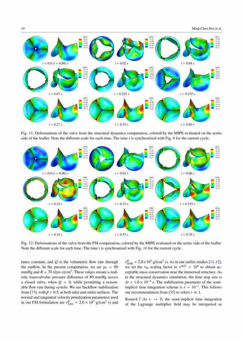
Fig. 11: Deformations of the valve from the structural dynamics computation, colored by the MIPE evaluated on the aorticside of the leaflet. Note the different scale for each time. The time t is synchronized with Fig. 9 for the current cycle.

t = 0.0 (t = 0.86) s t = 0.02 s t = 0.06 s

t = 0.24 s t = 0.33 s t = 0.335 s

t = 0.34 s t = 0.53 s t = 0.78 s

Fig. 12: Deformations of the valve from the FSI computation, colored by the MIPE evaluated on the aortic side of the leaflet.Note the different scale for each time. The time t is synchronized with Fig. 10 for the current cycle.

tance constant, and Q is the volumetric flow rate throughthe outflow. In the present computation, we set p0 = 80mmHg and R = 70 (dyn s)/cm5. These values ensure a real-istic transvalvular pressure difference of 80 mmHg acrossa closed valve, when Q = 0, while permitting a reason-able flow rate during systole. We use backflow stabilizationfrom [73], with β = 0.5, at both inlet and outlet surfaces. Thenormal and tangential velocity penalization parameters usedin our FSI formulation are τB

TAN = 2.0 × 103 g/(cm2 s) and

τBNOR = 2.0×102 g/(cm2 s). As in our earlier studies [11,12],

we set the τM scaling factor to sshell = 106 to obtain ac-ceptable mass conservation near the immersed structure. Asin the structural dynamics simulation, the time step size is∆t = 1.0 × 10−4 s. The stabilization parameter of the semi-implicit time integration scheme is r = 10−5. This followsour recommendation from [35] to select r � 1.

Remark 7 As r → 0, the semi-implicit time integrationof the Lagrange multiplier field may be interpreted as

Title Suppressed Due to Excessive Length 11

t = 0.0 (t = 0.86) s t = 0.02 s t = 0.06 s t = 0.24 s t = 0.33 s

t = 0.335 s t = 0.34 s t = 0.38 s t = 0.53 s t = 0.78 s

Fig. 13: Volume rendering of the velocity field at several points during a cardiac cycle. The time t is synchronized withFig. 10 for the current cycle.

a fully-implicit fluid–structure displacement penalization(cf. [11, Section 4.2.1]), with stiffness τB

NOR/∆t = 2.0 × 107

dyn/cm3. We may roughly estimate the physical signifi-cance of the time step splitting error incurred through semi-implicit integration by considering the fluid displacementthrough the valve in static equilibrium. The fluid wouldpenetrate through the closed valve by a distance of only∆P/(τNOR/∆t) = 0.005 cm for diastolic pressure differenceson the order of ∆P = 105 dyn/cm2. This is effectively withinmodeling error, considering that the penetration is nearly anorder of magnitude smaller than the thickness of the leaflets.

3.3.3 Results and discussion

Fig. 11 illustrates the deformations and strain distributionsof the BHV model throughout a period of the prescribedpressure loading. Fig. 12 shows the deformations and strainsfrom a period of the FSI simulation, while Fig. 13 depictsthe corresponding flow fields in the artery lumen. The volu-metric flow rate through the top of the artery throughout thecardiac cycle is shown in Fig. 14.

Several important qualitative differences between thevalve deformations in the dynamic and FSI computations are

Time (s)

Flow

rate

(mL/

s)

0 0.1 0.2 0.3 0.4 0.5 0.6 0.7 0.8

-100

0

100

200

300

400

500

Fig. 14: Computed volumetric flow rate through the top ofthe fluid domain, during a full cardiac cycle of 0.86 s.

observed. Firstly, the opening process is very different. Wecan see from the snapshots at t = 0.02 s from Figs. 11 and 12that the follower load in the dynamic computation drives thefree edges of the leaflets apart immediately, while, in theFSI computation, the opening deformation initiates near the

12 Ming-Chen Hsu et al.

attached edge, then spreads toward the free edge. The open-ing of the leaflets in the FSI computation closely resemblesthe sequence of pericardial BHV leaflet deformations mea-sured in vitro in [106], while the dynamic simulation ex-hibits unrealistic features. It is clear from the deformationcross-sections in Fig. 15 that a portion of the leaflet nearthe free edge ends up with the top (aortic) side of the leafletfacing downward. The follower load then pushes the freeedge downward, exaggerating this feature. A similar artifactis apparent in the earlier dynamic computations of [31,101].

During the closing phase, the coaptation of the freeedges of the leaflets is significantly delayed in the FSI com-putation; the free edges lean outward throughout the clos-ing process, as is clear in Fig. 15. The follower load of thedynamic simulation drives the leaflets closed in a more uni-form manner. This delayed closing of the free edge occursin some pericardial bioprosthetic valve leaflets, and is evi-dent in the photographic images taken and reported in [104].This deformation is not observed in all valve leaflets, though(cf. [106]), and we therefore suspect that it is highly sensi-tive to valve geometry, leaflet material properties, and flow

0

5

70 203040

225

235

270

Unit: ms

Fullyclosed

Fullyopened

350

Structural dynamics (SD)

015

20

2560240

330

335

340

530

Unit: ms

Fullyclosed

Fullyopened

FSI

Fully closed

240

Fullyopened

530

60

70350

0

Unit: msComparison between SD and FSI

Fig. 15: Cross-sections of the time-dependent leaflet profile.

conditions. It seems unlikely that a uniform pressure fol-lower load would cause this closing behavior, and it is notseen in any of the earlier structural dynamics computationsof [9, 31, 101].

For the fully-closed configuration, the structural dynam-ics and FSI simulation results are quite similar, as can beseen in Fig. 15. Fig. 13 shows that at this configuration, theflow is nearly hydrostatic. The BHV in the FSI computa-tion is under hydrostatic pressure, which is at a similar levelto the prescribed pressure load applied in the structural dy-namics simulation. This result shows the applicability of thecommon modeling practice of approximating the influenceof the fluid on the fully-closed valve as a pressure followerload, even though at other phases clear discrepancies wereobserved between dynamic and FSI computations.

4 Conclusions and further work

In this work we combine the geometry modeling and para-metric design platform introduced in [19], thin shell con-stitutive modeling framework developed in [22], and im-mersogeometric FSI methodology proposed in [11, 12] toperform high-fidelity BHV FSI with a greater level of au-tomation, robustness and realism than achieved previously.We demonstrate the performance of our methods by apply-ing them to a challenging problem of FSI analysis of BHVsat full scale and with full physiological realism. We illus-trate the added value of including realistic material modelsof leaflet tissue and FSI coupling by comparing our resultswith those that omit material nonlinearity, or approximatethe influence of the blood flow on the structure by meansof applying prescribed uniform pressure loads and dampingforces. The present effort represents the first step toward au-tomated optimization of the leaflet design, to increase theuseful life of BHVs.

Acknowledgements M.S. Sacks was supported by NIH/NHLBI grantR01 HL108330. D. Kamensky was partially supported by the CSEMGraduate Fellowship. M.-C. Hsu, C. Wang and Y. Bazilevs were par-tially supported by the ARO grant No. W911NF-14-1-0296. J. Kiendland A. Reali were partially supported by the European Research Coun-cil through the FP7 Ideas Starting Grant No. 259229 ISOBIO. Wethank the Texas Advanced Computing Center (TACC) at the Universityof Texas at Austin for providing HPC resources that have contributedto the research results reported in this paper.

References

1. F. J. Schoen and R. J. Levy. Calcification of tissue heart valvesubstitutes: progress toward understanding and prevention. Ann.Thorac. Surg., 79(3):1072–1080, 2005.

2. P. Pibarot and J. G. Dumesnil. Prosthetic heart valves: selectionof the optimal prosthesis and long-term management. Circula-tion, 119(7):1034–1048, 2009.

Title Suppressed Due to Excessive Length 13

3. C.-P. Li, S.-F. Chen, C.-W. Lo, and P.-C. Lu. Turbulence charac-teristics downstream of a new trileaflet mechanical heart valve.ASAIO Journal, 57(3):188–196, 2011.

4. B. M. Yun, J. Wu, H. A. Simon, S. Arjunon, F. Sotiropoulos,C. K. Aidun, and A. P. Yoganathan. A numerical investigationof blood damage in the hinge area of aortic bileaflet mechani-cal heart valves during the leakage phase. Annals of BiomedicalEngineering, 40(7):1468–1485, 2012.

5. R. F. Siddiqui, J. R. Abraham, and J. Butany. Bioprosthetic heartvalves: modes of failure. Histopathology, 55:135–144, 2009.

6. M. S. Sacks and F. J. Schoen. Collagen fiber disruption occursindependent of calcification in clinically explanted bioprostheticheart valves. J. Biomed. Mater. Res., 62(3):359–371, 2002.

7. M. S. Sacks, A. Mirnajafi, W. Sun, and P. Schmidt. Biopros-thetic heart valve heterograft biomaterials: structure, mechanicalbehavior and computational simulation. Expert Rev Med De-vices, 3(6):817–834, 2006.

8. W. Sun, A. Abad, and M. S. Sacks. Simulated bioprosthetic heartvalve deformation under quasi-static loading. Journal of Biome-chanical Engineering, 127(6):905–914, 2005.

9. A. F. Saleeb, A. Kumar, and V. S. Thomas. The important rolesof tissue anisotropy and tissue-to-tissue contact on the dynamicalbehavior of a symmetric tri-leaflet valve during multiple cardiacpressure cycles. Med Eng Phys, 35(1):23–35, 2013.

10. F. Auricchio, M. Conti, A. Ferrara, S. Morganti, and A. Reali.Patient-specific simulation of a stentless aortic valve implant:the impact of fibres on leaflet performance. Computer Methodsin Biomechanics and Biomedical Engineering, 17(3):277–285,2014.

11. D. Kamensky, M.-C. Hsu, D. Schillinger, J. A. Evans, A. Aggar-wal, Y. Bazilevs, M. S. Sacks, and T. J. R. Hughes. An immerso-geometric variational framework for fluid–structure interaction:Application to bioprosthetic heart valves. Computer Methods inApplied Mechanics and Engineering, 284:1005–1053, 2015.

12. M.-C. Hsu, D. Kamensky, Y. Bazilevs, M. S. Sacks, and T. J. R.Hughes. Fluid–structure interaction analysis of bioprostheticheart valves: significance of arterial wall deformation. Computa-tional Mechanics, 54:1055–1071, 2014.

13. C. S. Peskin. Flow patterns around heart valves: A numeri-cal method. Journal of Computational Physics, 10(2):252–271,1972.

14. C. S. Peskin. The immersed boundary method. Acta Numerica,11:479–517, 2002.

15. R. Mittal and G. Iaccarino. Immersed boundary methods. AnnualReview of Fluid Mechanics, 37:239–261, 2005.

16. F. Sotiropoulos and X. Yang. Immersed boundary methods forsimulating fluid–structure interaction. Progress in AerospaceSciences, 65:1–21, 2014.

17. T. J. R. Hughes, J. A. Cottrell, and Y. Bazilevs. Isogeometricanalysis: CAD, finite elements, NURBS, exact geometry, andmesh refinement. Computer Methods in Applied Mechanics andEngineering, 194:4135–4195, 2005.

18. J. A. Cottrell, T. J. R. Hughes, and Y. Bazilevs. IsogeometricAnalysis: Toward Integration of CAD and FEA. Wiley, Chich-ester, 2009.

19. M.-C. Hsu, C. Wang, A. G. Herrema, D. Schillinger, A. Ghoshal,and Y. Bazilevs. An interactive geometry modeling and para-metric design platform for isogeometric analysis. Computers &Mathematics with Applications, 2015. http://dx.doi.org/10.1016/

j.camwa.2015.04.002.20. J. Kiendl, K.-U. Bletzinger, J. Linhard, and R. Wuchner. Isoge-

ometric shell analysis with Kirchhoff–Love elements. ComputerMethods in Applied Mechanics and Engineering, 198:3902–3914, 2009.

21. J. Kiendl, Y. Bazilevs, M.-C. Hsu, R. Wuchner, and K.-U.Bletzinger. The bending strip method for isogeometric anal-ysis of Kirchhoff–Love shell structures comprised of multiple

patches. Computer Methods in Applied Mechanics and Engi-neering, 199:2403–2416, 2010.

22. J. Kiendl, M.-C. Hsu, M. C. H. Wu, and A. Reali. IsogeometricKirchhoff–Love shell formulations for general hyperelastic mate-rials. Computer Methods in Applied Mechanics and Engineering,2015. http://dx.doi.org/10.1016/j.cma.2015.03.010.

23. Rhinoceros. http://www.rhino3d.com/. 2015.24. Autodesk T-Splines Plug-in for Rhino. http://www.tsplines.com/

products/tsplines-for-rhino.html. 2015.25. L. Piegl and W. Tiller. The NURBS Book (Monographs in Visual

Communication), 2nd ed. Springer-Verlag, New York, 1997.26. M. A. Scott, T. J. R. Hughes, T. W. Sederberg, and M. T. Seder-

berg. An integrated approach to engineering design and analy-sis using the Autodesk T-spline plugin for Rhino3d. ICES RE-PORT 14-33, The Institute for Computational Engineering andSciences, The University of Texas at Austin, September 2014,2014.

27. X. Li, J. Zheng, T. W. Sederberg, T. J. R. Hughes, and M. A.Scott. On linear independence of T-spline blending functions.Computer Aided Geometric Design, 29(1):63–76, 2012.

28. X. Li and M. A. Scott. Analysis-suitable T-splines: Characteriza-tion, refineability, and approximation. Mathematical Models andMethods in Applied Sciences, 24:1141–1164, 2014.

29. Grasshopper. http://www.grasshopper3d.com/. 2015.30. Rhino Developer Tools. http://wiki.mcneel.com/developer/

home. 2015.31. H. Kim, J. Lu, M. S. Sacks, and K. B. Chandran. Dynamic sim-

ulation of bioprosthetic heart valves using a stress resultant shellmodel. Annals of Biomedical Engineering, 36(2):262–275, 2008.

32. T. W. Sederberg, D. L. Cardon, G. T. Finnigan, N. S. North,J. Zheng, and T. Lyche. T-spline simplification and local refine-ment. ACM Transactions on Graphics, 23(3):276–283, 2004.

33. G. A. Holzapfel. Nonlinear Solid Mechanics: A Continuum Ap-proach for Engineering. Wiley, Chichester, 2000.

34. M. A. Scott, M. J. Borden, C. V. Verhoosel, T. W. Sederberg,and T. J. R. Hughes. Isogeometric finite element data structuresbased on Bezier extraction of T-splines. International Journalfor Numerical Methods in Engineering, 88:126–156, 2011.

35. D. Kamensky, J. A. Evans, and M.-C. Hsu. Stability and con-servation properties of collocated constraints in immersogeomet-ric fluid–thin structure interaction analysis. Communications inComputational Physics, 2015. Accepted.

36. T. J. R. Hughes, W. K. Liu, and T. K. Zimmermann. Lagrangian–Eulerian finite element formulation for incompressible viscousflows. Computer Methods in Applied Mechanics and Engineer-ing, 29:329–349, 1981.

37. J. Donea, S. Giuliani, and J. P. Halleux. An arbitrary Lagrangian–Eulerian finite element method for transient dynamic fluid–structure interactions. Computer Methods in Applied Mechanicsand Engineering, 33(1-3):689–723, 1982.

38. L. Formaggia, J. F. Gerbeau, F. Nobile, and A. Quarteroni. On thecoupling of 3D and 1D Navier-Stokes equations for flow prob-lems in compliant vessels. Computer Methods in Applied Me-chanics and Engineering, 191:561–582, 2001.

39. J.-F. Gerbeau, M. Vidrascu, and P. Frey. Fluid–structure inter-action in blood flows on geometries based on medical imaging.Computers and Structures, 83:155–165, 2005.

40. F. Nobile and C. Vergara. An effective fluid–structure interactionformulation for vascular dynamics by generalized Robin condi-tions. SIAM Journal on Scientific Computing, 30:731–763, 2008.

41. Y. Bazilevs, M.-C. Hsu, Y. Zhang, W. Wang, X. Liang, T. Kvams-dal, R. Brekken, and J. Isaksen. A fully-coupled fluid–structureinteraction simulation of cerebral aneurysms. ComputationalMechanics, 46:3–16, 2010.

42. Y. Bazilevs, M.-C. Hsu, Y. Zhang, W. Wang, T. Kvamsdal,S. Hentschel, and J. Isaksen. Computational fluid–structure inter-action: Methods and application to cerebral aneurysms. Biome-chanics and Modeling in Mechanobiology, 9:481–498, 2010.

14 Ming-Chen Hsu et al.

43. M. Perego, A. Veneziani, and C. Vergara. A variational approachfor estimating the compliance of the cardiovascular tissue: An in-verse fluid–structure interaction problem. SIAM Journal on Sci-entific Computing, 33:1181–1211, 2011.

44. M.-C. Hsu and Y. Bazilevs. Blood vessel tissue prestress mod-eling for vascular fluid–structure interaction simulations. FiniteElements in Analysis and Design, 47:593–599, 2011.

45. K. Takizawa, Y. Bazilevs, and T. E. Tezduyar. Space–time andALE–VMS techniques for patient-specific cardiovascular fluid–structure interaction modeling. Archives of Computational Meth-ods in Engineering, 19:171–225, 2012.

46. K. Takizawa, Y. Bazilevs, T. E. Tezduyar, C. C. Long, A. L.Marsden, and K. Schjodt. ST and ALE-VMS methods forpatient-specific cardiovascular fluid mechanics modeling. Math-ematical Models and Methods in Applied Sciences, 24:2437–2486, 2014.

47. T. E. Tezduyar. Stabilized finite element formulations for incom-pressible flow computations. Advances in Applied Mechanics,28:1–44, 1992.

48. T. E. Tezduyar. Computation of moving boundaries and inter-faces and stabilization parameters. International Journal for Nu-merical Methods in Fluids, 43:555–575, 2003.

49. T. E. Tezduyar and S. Sathe. Modelling of fluid–structure inter-actions with the space–time finite elements: Solution techniques.International Journal for Numerical Methods in Fluids, 54(6–8):855–900, 2007.

50. K. Takizawa and T. E. Tezduyar. Multiscale space–time fluid–structure interaction techniques. Computational Mechanics,48:247–267, 2011.

51. K. Takizawa and T. E. Tezduyar. Space-time fluid–structure in-teraction methods. Mathematical Models and Methods in Ap-plied Sciences, 22:1230001, 2012.

52. K. Takizawa, K. Schjodt, A. Puntel, N. Kostov, and T. E. Tezdu-yar. Patient-specific computational analysis of the influence of astent on the unsteady flow in cerebral aneurysms. ComputationalMechanics, 51:1061–1073, 2013.

53. K. Takizawa, T. E. Tezduyar, A. Buscher, and S. Asada. Space–time interface-tracking with topology change (ST-TC). Compu-tational Mechanics, 54:955–971, 2014.

54. K. Takizawa, R. Torii, H. Takagi, T. E. Tezduyar, and X. Y.Xu. Coronary arterial dynamics computation with medical-image-based time-dependent anatomical models and element-based zero-stress state estimates. Computational Mechanics,54:1047–1053, 2014.

55. K. Takizawa, T. E. Tezduyar, A. Buscher, and S. Asada. Space–time fluid mechanics computation of heart valve models. Com-putational Mechanics, 54:973–986, 2014.

56. Y. Bazilevs, V. M. Calo, Y. Zhang, and T. J. R. Hughes. Iso-geometric fluid–structure interaction analysis with applicationsto arterial blood flow. Computational Mechanics, 38:310–322,2006.

57. Y. Bazilevs, V. M. Calo, T. J. R. Hughes, and Y. Zhang. Isoge-ometric fluid–structure interaction: theory, algorithms, and com-putations. Computational Mechanics, 43:3–37, 2008.

58. Y. Bazilevs, M.-C. Hsu, K. Takizawa, and T. E. Tezduyar. ALE–VMS and ST–VMS methods for computer modeling of wind-turbine rotor aerodynamics and fluid–structure interaction. Math-ematical Models and Methods in Applied Sciences, 22:1230002,2012.

59. K. Takizawa, Y. Bazilevs, T. E. Tezduyar, M.-C. Hsu, O. Øiseth,K. M. Mathisen, N. Kostov, and S. McIntyre. Engineeringanalysis and design with ALE–VMS and Space–Time methods.Archives of Computational Methods in Engineering, 21:481–508, 2014.

60. Y. Bazilevs, K. Takizawa, T. E. Tezduyar, M.-C. Hsu, N. Kostov,and S. McIntyre. Aerodynamic and FSI analysis of wind tur-bines with the ALE–VMS and ST–VMS methods. Archives ofComputational Methods in Engineering, 21:359–398, 2014.

61. A. N. Brooks and T. J. R. Hughes. Streamline upwind/Petrov-Galerkin formulations for convection dominated flows with par-ticular emphasis on the incompressible Navier-Stokes equa-tions. Computer Methods in Applied Mechanics and Engineer-ing, 32:199–259, 1982.

62. T. E. Tezduyar and Y. Osawa. Finite element stabilization param-eters computed from element matrices and vectors. ComputerMethods in Applied Mechanics and Engineering, 190:411–430,2000.

63. T. J. R. Hughes, L. Mazzei, and K. E. Jansen. Large eddy sim-ulation and the variational multiscale method. Computing andVisualization in Science, 3:47–59, 2000.

64. T. J. R. Hughes, L. Mazzei, A. A. Oberai, and A. Wray. Themultiscale formulation of large eddy simulation: Decay of ho-mogeneous isotropic turbulence. Physics of Fluids, 13:505–512,2001.

65. T. J. R. Hughes, G. Scovazzi, and L. P. Franca. Multiscale andstabilized methods. In E. Stein, R. de Borst, and T. J. R. Hughes,editors, Encyclopedia of Computational Mechanics, Volume 3:Fluids, chapter 2. John Wiley & Sons, 2004.

66. Y. Bazilevs, V. M. Calo, J. A. Cottrel, T. J. R. Hughes, A. Re-ali, and G. Scovazzi. Variational multiscale residual-based tur-bulence modeling for large eddy simulation of incompressibleflows. Computer Methods in Applied Mechanics and Engineer-ing, 197:173–201, 2007.

67. M.-C. Hsu, Y. Bazilevs, V. M. Calo, T. E. Tezduyar, and T. J. R.Hughes. Improving stability of stabilized and multiscale formu-lations in flow simulations at small time steps. Computer Meth-ods in Applied Mechanics and Engineering, 199:828–840, 2010.

68. Y. Bazilevs, M.-C. Hsu, and M. A. Scott. Isogeometric fluid–structure interaction analysis with emphasis on non-matchingdiscretizations, and with application to wind turbines. ComputerMethods in Applied Mechanics and Engineering, 249–252:28–41, 2012.

69. P. Wriggers. Computational Contact Mechanics, 2nd ed.Springer-Verlag, Berlin Heidelberg, 2006.

70. T. A. Laursen. Computational Contact and Impact Mechanics:Fundamentals of Modeling Interfacial Phenomena in NonlinearFinite Element Analysis. Springer-Verlag, Berlin Heidelberg,2003.

71. S. Morganti, F. Auricchio, D. J. Benson, F. I. Gambarin, S. Hart-mann, T. J. R. Hughes, and A. Reali. Patient-specific isogeomet-ric structural analysis of aortic valve closure. Computer Methodsin Applied Mechanics and Engineering, 284:508–520, 2015.

72. Y. Bazilevs, J. R. Gohean, T. J. R. Hughes, R. D. Moser, andY. Zhang. Patient-specific isogeometric fluid–structure interac-tion analysis of thoracic aortic blood flow due to implantation ofthe Jarvik 2000 left ventricular assist device. Computer Methodsin Applied Mechanics and Engineering, 198:3534–3550, 2009.

73. M. Esmaily-Moghadam, Y. Bazilevs, T.-Y. Hsia, I. E. Vignon-Clementel, A. L. Marsden, and MOCHA. A comparison of outletboundary treatments for prevention of backflow divergence withrelevance to blood flow simulations. Computational Mechanics,48:277–291, 2011.

74. J. Chung and G. M. Hulbert. A time integration algorithm forstructural dynamics with improved numerical dissipation: Thegeneralized-α method. Journal of Applied Mechanics, 60:371–75, 1993.

75. K. E. Jansen, C. H. Whiting, and G. M. Hulbert. A generalized-αmethod for integrating the filtered Navier-Stokes equations witha stabilized finite element method. Computer Methods in AppliedMechanics and Engineering, 190:305–319, 2000.

76. T. E. Tezduyar, S. Sathe, and K. Stein. Solution techniques for thefully-discretized equations in computation of fluid–structure in-teractions with the space–time formulations. Computer Methodsin Applied Mechanics and Engineering, 195:5743–5753, 2006.

Title Suppressed Due to Excessive Length 15

77. T. E. Tezduyar, S. Sathe, R. Keedy, and K. Stein. Space–timefinite element techniques for computation of fluid–structure in-teractions. Computer Methods in Applied Mechanics and Engi-neering, 195:2002–2027, 2006.

78. T. E. Tezduyar and S. Sathe. Modeling of fluid–structure inter-actions with the space–time finite elements: Solution techniques.International Journal for Numerical Methods in Fluids, 54:855–900, 2007.

79. Y. Bazilevs, K. Takizawa, and T. E. Tezduyar. ComputationalFluid–Structure Interaction: Methods and Applications. Wiley,Chichester, 2013.

80. T. E. Tezduyar, K. Takizawa, C. Moorman, S. Wright, andJ. Christopher. Space–time finite element computation of com-plex fluid–structure interactions. International Journal for Nu-merical Methods in Fluids, 64:1201–1218, 2010.

81. T. E. Tezduyar. Finite element methods for flow problems withmoving boundaries and interfaces. Archives of ComputationalMethods in Engineering, 8:83–130, 2001.

82. J. E. Akin, T. E. Tezduyar, and M. Ungor. Computation of flowproblems with the mixed interface-tracking/interface-capturingtechnique (MITICT). Computers & Fluids, 36:2–11, 2007.

83. M. A. Cruchaga, D. J. Celentano, and T. E. Tezduyar. A nu-merical model based on the Mixed Interface-Tracking/Interface-Capturing Technique (MITICT) for flows with fluid–solid andfluid–fluid interfaces. International Journal for Numerical Meth-ods in Fluids, 54:1021–1030, 2007.

84. I. Akkerman, Y. Bazilevs, D. J. Benson, M. W. Farthing, andC. E. Kees. Free-surface flow and fluid–object interaction mod-eling with emphasis on ship hydrodynamics. Journal of AppliedMechanics, accepted for publication, 2011.

85. T. Wick. Flapping and contact FSI computations with the fluid–solid interface-tracking/interface-capturing technique and meshadaptivity. Computational Mechanics, 53(1):29–43, 2014.

86. T. Tezduyar, S. Aliabadi, M. Behr, A. Johnson, and S. Mit-tal. Parallel finite-element computation of 3D flows. Computer,26(10):27–36, 1993.

87. A. A. Johnson and T. E. Tezduyar. Mesh update strategies in par-allel finite element computations of flow problems with movingboundaries and interfaces. Computer Methods in Applied Me-chanics and Engineering, 119:73–94, 1994.

88. K. Stein, T. Tezduyar, and R. Benney. Mesh moving techniquesfor fluid–structure interactions with large displacements. Journalof Applied Mechanics, 70:58–63, 2003.

89. K. Stein, T. E. Tezduyar, and R. Benney. Automatic mesh up-date with the solid-extension mesh moving technique. ComputerMethods in Applied Mechanics and Engineering, 193:2019–2032, 2004.

90. Y. Bazilevs and T. J. R. Hughes. Weak imposition of Dirichletboundary conditions in fluid mechanics. Computers and Fluids,36:12–26, 2007.

91. Y. Bazilevs, C. Michler, V. M. Calo, and T. J. R. Hughes.Weak Dirichlet boundary conditions for wall-bounded turbulentflows. Computer Methods in Applied Mechanics and Engineer-ing, 196:4853–4862, 2007.

92. Y. Bazilevs, C. Michler, V. M. Calo, and T. J. R. Hughes. Isogeo-metric variational multiscale modeling of wall-bounded turbulentflows with weakly enforced boundary conditions on unstretchedmeshes. Computer Methods in Applied Mechanics and Engineer-ing, 199:780–790, 2010.

93. M.-C. Hsu, I. Akkerman, and Y. Bazilevs. Wind turbine aerody-namics using ALE–VMS: Validation and the role of weakly en-forced boundary conditions. Computational Mechanics, 50:499–511, 2012.

94. P. Tong and Y.-C. Fung. The stress-strain relationship for theskin. Journal of Biomechanics, 9(10):649 – 657, 1976.

95. Y. C. Fung. Biomechanics: Mechanical Properties of Living Tis-sues. Springer-Verlag, New York, second edition, 1993.

96. W. Sun, M. S. Sacks, T. L. Sellaro, W. S. Slaughter, and M. J.Scott. Biaxial mechanical response of bioprosthetic heart valvebiomaterials to high in-plane shear. Journal of BiomechanicalEngineering, 125(3):372–380, 2003.

97. R. Fan and M. S. Sacks. Simulation of planar soft tissues using astructural constitutive model: Finite element implementation andvalidation. Journal of Biomechanics, 47(9):2043–2054, 2014.

98. A. Mirnajafi, J. Raymer, M. J. Scott, and M. S. Sacks. The effectsof collagen fiber orientation on the flexural properties of peri-cardial heterograft biomaterials. Biomaterials, 26(7):795–804,2005.

99. H. Kim, K. B. Chandran, M. S. Sacks, and J. Lu. An experimen-tally derived stress resultant shell model for heart valve dynamicsimulations. Annals of Biomedical Engineering, 35(1):30–44,2007.

100. K. Li and W. Sun. Simulated thin pericardial bioprosthetic valveleaflet deformation under static pressure-only loading conditions:implications for percutaneous valves. Annals of Biomedical En-gineering, 38(8):2690–2701, 2010.

101. G. Burriesci, I. C. Howard, and E. A. Patterson. Influence ofanisotropy on the mechanical behaviour of bioprosthetic heartvalves. J Med Eng Technol, 23(6):203–215, 1999.

102. V. L. Huynh, T. Nguyen, H. L. Lam, X. G. Guo, and R. Kafesjian.Cloth-covered stents for tissue heart valves, 2003. US Patent6,585,766.

103. N. Piazza, S. Bleiziffer, G. Brockmann, R. Hendrick, M. A.Deutsch, A. Opitz, D. Mazzitelli, P. Tassani-Prell, C. Schreiber,and R. Lange. Transcatheter aortic valve implantation for fail-ing surgical aortic bioprosthetic valve. JACC: CardiovascularInterventions, 4(7):721–732, 2011.

104. Z. B. Gao, S. Pandya, N. Hosein, M. S. Sacks, and N. H. C.Hwang. Bioprosthetic heart valve leaflet motion monitored bydual camera stereo photogrammetry. Journal of Biomechanics,33(2):199–207, 2000.

105. B. Z. Gao, S. Pandya, C. Arana, and N. H. C. Hwang. Bio-prosthetic heart valve leaflet deformation monitored by double-pulse stereo photogrammetry. Annals of Biomedical Engineer-ing, 30(1):11–18, 2002.

106. A. K. S. Iyengar, H. Sugimoto, D. B. Smith, and M. S. Sacks. Dy-namic in vitro quantification of bioprosthetic heart valve leafletmotion using structured light projection. Annals of BiomedicalEngineering, 29(11):963–973, 2001.

107. B. J. Bellhouse and F. H. Bellhouse. Mechanism of closure ofthe aortic valve. Nature, 217(5123):86–87, 1968.

108. J. C. Simo and T. J. R. Hughes. Computational Inelasticity.Springer-Verlag, New York, 1998.

109. T. Kenner. The measurement of blood density and its meaning.Basic Research in Cardiology, 84(2):111–124, 1989.

110. R. Rosencranz and S. A. Bogen. Clinical laboratory measure-ment of serum, plasma, and blood viscosity. American Journalof Clinical Pathology, 125:S78–S86, 2006.

111. C. H. Yap, N. Saikrishnan, G. Tamilselvan, and A. P. Yoganathan.Experimental technique of measuring dynamic fluid shear stresson the aortic surface of the aortic valve leaflet. Journal of Biome-chanical Engineering, 133(6):061007, 2011.