dynamic effects of total debt and gdp: a time-series...
TRANSCRIPT

Dynamic Effects of Total Debt and GDP: A Time-SeriesAnalysis of the United States
Economics
Master's thesis
Patrizio Lainà
2011
Department of EconomicsAalto UniversitySchool of Economics

ABSTRACT
The purpose of the present thesis is to examine the dynamic interactions between total debt and
GDP. In particular, the growth rates are studied in real terms. Total debt is defined as the sum of
credit market liabilities of household, business, financial, foreign, federal government, state gov-
ernment and local government sectors.
The methodology of this study is based on time-series regression analysis, in which a structural
VAR model is estimated. Then, the dynamic interactions are studied with Granger causality tests,
impulse response functions and forecast error variance decompositions. The data is based on the
United States from 1959 to 2010 and it is organized quarterly.
The main finding of this study is that real total debt growth affects real GDP growth, but there is no
feedback from real GDP growth to real total debt growth. The response of real GDP growth to a
shock in real total debt growth seems to be transitory, but the level effect might be persistent. In
both cases the effect is in the same direction. Thus, a positive shock in the growth rate of real total
debt has a transitory positive effect on real GDP growth rate, but may have a persistent positive ef-
fect on the level of real GDP.
The results of this study imply that economic growth typically requires accumulating total debt. In
other words, economic growth is very difficult to achieve when total debt is reduced. At the time
being, the private sector of the United States is already heavily indebted and, hence, it seems likely
that it is unwilling or unable to accumulate more debt. Consequently, during a recession the public
sector should borrow to stimulate the economy and enhance the repayment ability of the private
sector. Furthermore, the United States can be considered as a financially sovereign country, which
does not face an income constraint, it can also clear all its debt obligations at any given time and,
thus, it cannot drift into insolvency. However, present financial institutions set constraints for public
borrowing especially in Europe. Consequently, there might be a need to redesign European institu-
tions in order to facilitate public borrowing.
Keywords: total debt, GDP, real, growth, money, United States, structural VAR

TIIVISTELMÄ
Tämän pro gradu -tutkielman tarkoituksena on tarkastella kokonaisvelan ja BKT:n välisiä dynaami-
sia vaikutuksia. Kokonaisvelka on määritelty kotitalouksien, yritysten, finanssisektorin, ulkomaan
sektorin, liittovaltion hallinnon, osavaltion hallinnon ja paikallishallinnon yhteenlasketuiksi luotto-
markkinavastuiksi.
Tutkielman metodologiana on aikasarja-analyysi, jossa estimoidaan rakenteellinen VAR-malli. Dy-
naamisia keskinäisvaikutuksia arvioidaan Granger kausaliteetin, impulssivastefunktioiden ja ennus-
tevirheiden varianssien pilkkomisen avulla. Aineisto perustuu Yhdysvaltoihin aikavälillä 1959–
2010 ja se on neljännesvuosittaista.
Tämän tutkielman tärkein havainto on, että reaalinen kokonaisvelan kasvu vaikuttaa reaaliseen
BKT:n kasvuun, mutta reaalinen BKT:n kasvu ei vaikuta reaaliseen kokonaisvelan kasvuun. Reaali-
sen BKT:n kasvun reaktio reaalisessa kokonaisvelan kasvussa tapahtuvaan shokkiin on väliaikai-
nen, mutta tasovaikutus saattaa olla pysyvä. Molemmissa tapauksissa vaikutus on samansuuntainen.
Niinpä positiivinen shokki reaaliseen kokonaisvelan kasvuun vaikuttaa väliaikaisesti positiivisesti
myös reaaliseen BKT:n kasvuun, mutta shokilla voi olla pysyvä positiivinen vaikutus reaaliseen
BKT:n tasoon.
Tutkielman tulokset viittaavat siihen, että tavallisesti talouskasvu vaatii kokonaisvelan kerryttämis-
tä. Talouskasvua on toisin sanoen hyvin vaikeaa saavuttaa kun kokonaisvelkaa vähennetään. Tällä
hetkellä Yhdysvaltojen yksityinen sektori on jo hyvin voimakkaasti velkaantunut, joten on epäto-
dennäköistä että se haluaisi tai pystyisi kerryttämään lisää velkaa. Niinpä taantuman aikana julkisen
sektorin täytyisikin lainata, jotta talous elpyisi ja yksityisen sektorin takaisinmaksukyky paranisi.
Lisäksi Yhdysvaltoja voidaan pitää taloudellisesti suvereenina valtiona, jonka kulutus ei ole tulora-
joitettua ja joka voi selvitä kaikista velkavelvoitteistaan kaikkina ajanhetkinä. Näin ollen Yhdysval-
lat ei voi ajautua maksukyvyttömyyteen. Nykyiset instituutiot kuitenkin asettavat rajoitteita julkisel-
le velkaantumiselle etenkin Euroopassa. Niinpä eurooppalaisia instituutioita täytyisikin uudistaa,
jotta julkinen velkaantuminen helpottuisi ja jotta taloutta voitaisiin näin tukea.
Avainsanat: kokonaisvelka, BKT, reaalinen, kasvu, raha, Yhdysvallat, rakenteellinen VAR

TABLE OF CONTENTS
1 INTRODUCTION ................................................................................................................... 1
1.1 Motivation ........................................................................................................................ 1
1.2 Central definitions ............................................................................................................. 1
1.3 Objectives ......................................................................................................................... 2
1.4 Findings ............................................................................................................................ 3
1.5 Structure ........................................................................................................................... 4
2 BACKGROUND ..................................................................................................................... 5
3 THEORETICAL FRAMEWORK .......................................................................................... 10
3.1 Financial instability hypothesis and debt deflation theory ................................................ 10
3.2 Endogenous money creation theory ................................................................................. 17
3.3 Modern money theory ..................................................................................................... 24
3.4 Monetary circuit theory ................................................................................................... 29
3.5 Related empirical studies ................................................................................................ 34
4 MODEL, DATA AND HYPOTHESES .................................................................................. 38
4.1 Model ............................................................................................................................. 38
4.2 Data description .............................................................................................................. 40
4.3 Hypotheses ..................................................................................................................... 46
5 ECONOMETRIC ANALYSIS ............................................................................................... 48
5.1 Total debt and GDP at a glance ....................................................................................... 48
5.2 Stationarity tests.............................................................................................................. 54
5.3 Cointegration tests .......................................................................................................... 56
5.4 Estimated regressions ...................................................................................................... 57
5.5 Granger causality tests .................................................................................................... 59
5.6 Impulse responses ........................................................................................................... 60
5.7 Variance decompositions ................................................................................................. 64

6 DISCUSSION ........................................................................................................................ 66
7 CONCLUSIONS ................................................................................................................... 74
7.1 Research summary .......................................................................................................... 74
7.2 Practical implications ...................................................................................................... 77
7.3 Limitations of the study .................................................................................................. 79
7.4 Suggestions for further research ...................................................................................... 81
REFERENCES ............................................................................................................................. 83
APPENDIX A: ECONOMETRIC METHODS ............................................................................. 91

LIST OF FIGURES
Figure 2.1 – Debt to GDP ratios in the United States ....................................................................... 6
Figure 2.2 – Growth rates of debt in the United States ..................................................................... 7
Figure 3.1 – Excess reserves in the United States .......................................................................... 19
Figure 3.2 – An extension of the monetary circuit theory ............................................................... 32
Figure 4.1 – Money aggregates and total debt................................................................................ 42
Figure 4.2 – Logarithmic levels of total debt and GDP .................................................................. 46
Figure 4.3 – Growth rates of total debt and GDP ........................................................................... 46
Figure 5.1 – Scatterplots for total debt and GDP ............................................................................ 49
Figure 5.2 – Real growth rates of total debt and GDP .................................................................... 50
Figure 5.3 – Autocorrelations of nominal variables........................................................................ 51
Figure 5.4 – Autocorrelations of real variables .............................................................................. 52
Figure 5.5 – Cross-correlations of total debt and GDP ................................................................... 53
Figure 5.6 – Impulse response functions ........................................................................................ 61
Figure 5.7 – Cumulative impulse response functions ..................................................................... 63
Figure 5.8 – Forecast error variance decompositions ..................................................................... 64
LIST OF TABLES
Table 4.1 – Summary statistics ...................................................................................................... 45
Table 5.1 – Augmented Dickey-Fuller tests ................................................................................... 55
Table 5.2 – Cointegration tests with Engle-Granger method .......................................................... 57
Table 5.3 – Granger causality tests ................................................................................................ 59

1
1 INTRODUCTION
1.1 Motivation
After a long period of accumulating debt the world has surged into a crisis. However, not many
years ago mainstream economists celebrated for solving the main problem causing depressions (see
e.g. Bernanke 2002 and Lucas 2003). This said, it is not surprising that the financial crisis was
unexpected by almost all economists. Nevertheless, some unorthodox economists were able to
predict the upcoming financial crisis using alternative indicators (see e.g. Keen 2001, 254 and
Roubini & Setser 2005). One of the most important indicators they used was debt.
The total debt to GDP (gross domestic product) ratio has been on an exponential trend path in the
United States ever since the 1970s. This development was not seen as alarming by most economists,
although they paid attention to inflation, interest rates, public debt to GDP ratio, money aggregates
and other relatively narrow quantity measures.
Traditionally, the interactions between money and economic activity have been studied (see e.g.
Sims 1972, Moore 1988, Friedman & Kuttner 1992, McCandless & Weber 1995 and Bernanke
2000). According to Minsky (1982 & 1986) and Adrian and Shin (2009 & 2011), however, in a
market-based financial system changes in purchasing power might not reflect to money supply
measures. This thesis holds total debt as a notably more comprehensive measure for aggregate
purchasing power of the economy. In addition, total debt captures also money supply measures as
all money is debt.
1.2 Central definitions
It is important to define and make a distinction between the concepts of money, debt, credit and
purchasing power. Innes (1913) defines money as the intermediate commodity in an exchange of a
commodity. Money is defined by Keen (2009) as a unit of account whose transfer is accepted as
final payment in all commodity and service exchanges. For practical reasons, however, this study
defines money as any money supply measure up to M3.

2
Debt is an obligation owed by one party to another party. In this study the obligation refers to assets
based on economic value and not to, for example, moral obligation. According to Innes (1913), the
words “credit” and “debt” express a legal relationship between two parties, but seen from two
opposite sides. Thus, debt is also credit, but it is called debt from the debtor's point of view, while it
is called credit from the creditor’s point of view. Consequently, in this study debt and credit are used
interchangeably.
Innes (1913) defines purchasing power simply as debt. That is, purchasing power is the flip side of
the legal obligation of debt to pay something back. To summarize, this study refers to purchasing
power, debt and credit interchangeably, while money is defined more narrowly.
In this thesis, however, the most commonly used concepts are total debt, private debt and public
debt. Private debt is defined as the sum of credit market liabilities of household, business, financial
and foreign sectors. Public debt, on the other hand, is defined as the sum of credit market liabilities
of federal government, state government and local government sectors. Total debt is simply the sum
of private debt and public debt.
1.3 Objectives
The purpose of this paper is to study the dynamic effects of total debt and GDP. In particular, the
rates of changes are analyzed in real terms. The methodology is based on econometric time-series
regression analysis, in which a two-variable structural vector autoregressive model is estimated. The
data is organized quarterly and it is from the United States between 1959 and 2010.
The present study is motivated by the following questions. Does total debt affect GDP? Does GDP
affect total debt? If either one does, what are the effects? Can we say anything about the causality?
In order to answer these questions three hypotheses are tested:
Hypothesis 1: Contemporaneous and past total debt affects contemporaneous GDP. In other
words, the hypothesis suggests that GDP is endogenous. This is assumed to be due to
contemporaneous and past total debt might determine production, consumption and public
spending possibilities.

3
Hypothesis 2: Past GDP affects contemporaneous total debt. In other words, the hypothesis
suggests that total debt is endogenous. This is assumed to be due to the possibility that past
GDP might be used as collateral for debt creation.
Hypothesis 3: GDP growth responds differently to a shock in total debt growth depending on
the time horizon. High (low) total debt growth might increase (decrease) GDP in the near
future, but it might decrease (increase) GDP in the distant future. This is supposed to be due
to changes in purchasing power and inflexible prices. Total debt growth might increase
economic activity in the near future as more purchasing power is created than returned. In
contrast, total debt growth might decrease economic activity in the distant future as more
purchasing power is returned than created as debts mature. In addition, hoarding
(precautionary saving) might be more common during high level of debt.
1.4 Findings
The main findings of this study show that contemporaneous and past real total debt growth seems to
affect contemporaneous real GDP growth. The response of real GDP growth to a shock in real total
debt growth seems to be transitory as the impulse response function converges to zero. However,
the level effect seems to be persistent as the cumulative impulse response function converges to a
statistically significant positive value. In both cases the effect is in the same direction. Thus, a
positive shock in the growth rate of real total debt has a transitory positive effect on real GDP
growth rate, but may have a persistent positive effect on the level of real GDP. Nevertheless, there
seems to be no feedback from past real GDP growth to contemporaneous real total debt growth as
impulse responses and variance decompositions are not statistically significant.
The main findings of this study support hypothesis 1, but reject hypothesis 2. The findings imply
that real GDP growth is endogenous, but real total debt growth is exogenous. The dynamic effects
are tested with Granger causality, impulse response functions and forecast error variance
decompositions. The findings of Granger causality tests are somewhat ambiguous. The results
neither support nor reject the possibility for bidirectional causality, unidirectional causality running
to either way or absence of any causal relation. On the other hand, the results of impulse responses
and variance decompositions are quite unambiguous. They all support unidirectional causality
running from real total debt to real GDP.

4
The findings of this study support the first part of hypothesis 3, which states that a shock in real
total debt growth affects real GDP growth in the same direction in the near future. However, the
latter part of the hypothesis does not receive support. Although a shock in real total debt growth
affects real GDP growth slightly in the opposite direction in the distant future, the response is not
statistically significant.
1.5 Structure
This thesis consists of seven chapters. This Chapter 1 gave an introductory to the topic. Chapter 2
gives a brief outlook to the background. Chapter 3 outlines the theoretical framework of this study
and presents some related empirical studies. Chapter 4 presents the model, describes the data and
constructs three hypotheses. Chapter 5 estimates and tests the model carefully. Chapter 6 discusses
and, finally, Chapter 7 draws some conclusions.

5
2 BACKGROUND
Again in the recent years, there has been a growing interest in depression economics due to the
ongoing financial crisis. However, not many years ago mainstream economists boldly declared that
the main problem, which causes depressions, has been solved (see e.g. Bernanke 2002 and Lucas
2003). This said, it is not surprising that the financial crisis was unexpected by almost all
economists. Nevertheless, some unorthodox economists were able to predict the upcoming financial
crisis using alternative indicators (see e.g. Keen 2001, 254 and Roubini & Setser 2005). Before
going through the development from housing and MBS crisis to public debt crisis and presenting
some illustrative figures, it should be pointed out that in this thesis financial crisis refers to all of
these developments described below and not only to the “first steps” of the crisis.
The present financial crisis began already in 2006, when housing prices in the United States began
to decline. This led to foreclosures as subprime borrowers could not service their mortgage debts.
As a consequence, the values of previously AAA-rated mortgage backed securities (MBS) crashed.
This led to defaults and bankruptcies. Also values of other stocks and derivatives declined, which
led to the housing and MBS crisis.
As the repayment ability of the borrowers deteriorated, banks had to write down debts from their
balance sheets. When the assets of the banks were devalued, it caused massive losses also for banks.
This led to the banking crisis. Banks could not proceed with their normal lending practices as the
uncertainty of the future grew and they had also insufficient capital.
The governments had to step in to recapitalize the banks and to take possession of some of the junk
loans. In addition, in economic downturn automatic stabilizers (such as increased spending in
unemployment) increased budget deficits. In order to finance the costs the governments were forced
to run into debt. However, regardless of the governments’ efforts the banks did not increase their
lending as it was perceived too risky. Moreover, debtors prepared to repay rather than accumulate
debt and potential debtors preferred to postpone their borrowing due to increased future uncertainty.
Thus, the real1 economy did not recover and the government had to stimulate that also. All this led
to the public debt crisis.
1 The term real is used in two different contexts. With total debt and GDP it refers to their values deflated by the CPI,
while with economy it refers to the production and consumption of goods and services.

6
To overcome the public debt crisis the governments have adopted austerity measures. However, it is
possible that the austerity measures further decrease economic activity as the private sector cannot
or will not go more into debt as it is already heavily indebted and the future looks gloomy. As debt
seems to be a key factor in all of these developments, next we will examine it in more detail.
In this thesis it is argued that traditionally economists have focused on studying public debt, but
they have not paid enough attention on private or total debt. Public debt (or sometimes referred as
government debt) is defined as total credit market liabilities of federal, state and local governments.
Private debt is defined as total credit market liabilities of household, business, financial and foreign2
sectors. Total debt is defined as the sum of private and public debts. Thus, total debt follows
Friedman’s (1981) definition, except it includes also foreign debt.
Figures 2.1 and 2.2 below show the development of debt in the United States from 1959 to 2010.
The figures examine both the level and the growth rate of debt.
Panel (A): Total debt Panel (B): Total debt decomposed
Figure 2.1 – Debt to GDP ratios in the United States
Sources: Federal Reserve (2010a), EconStats (2010) & U.S. Department of Commerce (2010).
As Figure 2.1 Panel (A) shows, the total debt to GDP ratio has been on exponential growth path
ever since the 1970s. It is worthwhile to point out that the nominal and real level of total debt have
been growing even more exponentially. Usually, it is perceived that the level of public debt to GDP
2 Foreign debt represents amount borrowed by foreign entities in U.S. markets only. All other debt components are
considered domestic and they comprise credit market funds borrowed by U.S. entities from both domestic and foreign
sources. For further details of these definitions see Federal Reserve (2010a). Foreign debt is considered as private
because it is probably mostly private, but also because, similarly as other private debt, it cannot be directly influenced
by the U.S. government. Nevertheless, foreign debt is by far the smallest component of total debt and thus has no
significant impact on the results.

7
should be stable. Actually, as Figure 2.1 Panel (B) shows, the public debt to GDP ratio has been
relatively stable during the last 50 years, while almost all private debt components compared to
GDP have been on a more or less exponential growth path. Clearly, the most notable accumulation
of debt has happened in the financial sector.
Interestingly, mainstream economists have given warnings about the public debt to GDP ratio (see
e.g. Sargent & Wallace 1981), but at the same time they have almost completely neglected the
private debt to GDP ratio. This might be due to Fama's (1965 & 1970) widely used efficient market
hypothesis, which simply implies that private debt does not matter because it is always on the
“right” level and no economic imbalances, such as bubbles3, should occur. This, in turn, indicates
that there is no need to study private or total debt. Keynes (1936) had previously argued that the
underlying assumptions in the efficient market hypothesis do not hold in reality and, instead, had
stressed that the future is essentially unknown. Although also Hahn (1966) and Samuelson (1967)
questioned Fama's efficient market hypothesis by arguing that even rational expectations and
market behavior do not rule out the possibility of bubbles, it seems that Fama's perception has been
more influential.
Panel (A): Total debt Panel (B): Total debt decomposed
Figure 2.2 – Growth rates of debt in the United States
Sources: Federal Reserve (2010a) & EconStats (2010).
Note: All variables have been smoothed with moving-average filter with four lags, one contemporaneous term and four forwards.
Figure 2.2 Panel (A) shows the recent radical deceleration of total debt growth. Figure 2.2 Panel (B)
illustrates that the growth rate of private debt has recently hit negative values for the first time
3 Stiglitz (1990) defines bubble with respect to economic fundaments. Thus, if prices are high today only because they
are expected to be even higher tomorrow, we can conclude that there exists a bubble.
8
between 1959 and 2010. The growth rate of public debt, in turn, has recently reached record levels.
We can clearly observe that private and public debt tend to behave in the opposite directions. Put
differently, when the growth rate of private debt slows down, the growth rate of public debt tends to
accelerate – and vice versa.
As has been described above, the typical solution to overcome a recession has been that the
government borrows as the private demand for and/or supply of debt has plummeted. It is a
standard Keynesian approach to stimulate the aggregate demand4 when there is an economic slump.
However, Figure 2.1 Panel (B) shows that the total public debt is smaller than household, business
or financial debt separately. In other words, as Figure 2.2 verifies, the behavior of private debt
clearly dominates total debt.
As the share of the public debt is only a minor fraction of total debt, the government borrowing –
aggressive as it has recently been – has not had a significant impact on total debt. It has barely kept
up the credit markets from collapsing, and prevented the economy from falling to a more serious
deflationary depression. In other words, the government has not been able to cure the crisis; it has
only succeeded to mitigate its effects.
Unfortunately, even the mitigation cannot be kept up forever as the indebtedness of the government
increases. In other words, public borrowing has its limits – at least within the prevailing financial
institutional framework. For example, the United States government has a debt ceiling, raising of
which needs to be passed in the congress, and the European Union (EU) member states are
constrained by the article 104 of the Maastricht Treaty, which limits their public debt to 60 % of
their GDP. In addition, EU member states are forbidden to borrow from the European Central Bank
(ECB). These measures are, in effect, arbitrary political decisions to restrict the financial
sovereignty of these countries.
Eventually, the indebtedness of the government seems to limit the Keynesian stimulation approach.
In addition, public borrowing might also have some effects on private borrowing. If the government
borrowed more, it could erode the confidence of the private sector on the repayment ability of the
government. Thus, the private sector might decrease borrowing as much or even more than the
government could increase it. This is the Ricardian equivalence theory. As a consequence, many
4 Sometimes it is argued that government borrowing also stimulates the aggregate supply as the government can
provide, for example, cheap credit for the firms in order to support the production process.

9
member states of the EU have already drifted to austerity measures and the United States seems to
follow. As Figure 2.2 Panel (B) illustrates, there is also a sign that the United States government
will limit its borrowing as the growth rate of government debt has already declined.
This perception is well captured in Europe, where a moralistic emphasis has characterized the crisis
debate. Others blame governments for getting too much into debt, while others blame the banks for
irresponsible lending practices. Nevertheless, both perspectives share the same premise that we
should have gotten less into debt. The debate is only about whom to blame: the demand for or the
supply of credit. Section 3.3 will give some revealing examples of public borrowing and
institutional design. Later in Chapter 5, we will scrutinize in more detail some aggregate effects of
“excessive” borrowing. The next chapter, however, will proceed to the theoretical framework of this
study.

10
3 THEORETICAL FRAMEWORK
This chapter presents the theoretical framework of this thesis and some related empirical studies.
First, the financial instability hypothesis and debt deflation theory are presented. Second, the
endogenous money creation theory is described. Third, the modern money theory is presented.
Fourth, the monetary circuit theory is outlined. Finally, some related empirical studies are
presented.
3.1 Financial instability hypothesis and debt deflation theory
The present section covers the basics of the financial instability hypothesis and the debt deflation
theory. These concepts were already touched in the previous chapter, but this section digs deeper
and focuses explicitly on these concepts. Next, the original versions of these theories are presented.
Later, some models and modern reformulations of these theories are presented.
The financial instability hypothesis was first advanced by Minsky (1982 & 1986), and the debt
deflation theory was developed by Fisher (1933) as an explanation for the Great Depression.
Actually, Minsky has incorporated the debt deflation theory as a part of his financial instability
hypothesis. Because of this reason, the financial instability hypothesis is presented first and then the
debt deflation theory is presented.
Minsky's (1982 & 1986) financial instability hypothesis holds that private debt is a key factor
influencing the real economy and the financial markets. Thus, Minsky's approach differs
significantly from Fama's (1965 & 1970) efficient market hypothesis. Minsky (1982 & 1986) argues
that the financial markets have a tendency to drift into a speculative phase, which is characterized
by rapid private debt growth and risky investments. Ultimately, this kind of development leads to a
financial crisis, which will start the process all over again. Minsky (1982 & 1986) believes that
economic crises can be seen as a historical continuum.
Minsky (1982 & 1986) presents the process of financial instability as follows:
1. The process starts from a situation where the real economy is healthy and growing. Firms
and financial institutions are, nevertheless, cautious and try to avoid risky investments due

11
to a crisis in the recent past.
2. However, low-risk investments keep on succeeding and economic growth accelerates.
Positive development of balance sheets inspires the firms and investors to take more risk as
it tends to be clearly profitable. More finance is needed and the banking sector loosens its
lending terms. In this situation both debtors and creditors see a bright future.
3. A self-reinforcing cycle is born as new debt money increases the demand for financial
assets, housing and other investments. Financial institutions loosen their lending terms more
and, for that reason, hedge, speculative and Ponzi borrowers appear on the market. First,
there appear the hedge borrowers. They can make debt repayments, covering interest and
principal, from the cash flows the investment produces. After the hedge borrowers,
speculative borrowers will appear. They can service the debt, that is, make interest
payments, but they must regularly roll over the principal. Finally, the Ponzi borrowers will
appear. They found their investment strategy on the assumption that asset values will keep
on rising. Ponzi borrowers cannot make sufficient payments on interest or principal from the
cash flows the investment provides, but they refinance the debt with the appreciated asset
value.
The increased demand for and supply of credit manifest in different ways depending on the
financial environment. In a regulated environment there will be a growth of non-bank
finances, while in a deregulated environment there will be a rapid increase in the money
supply. Alternatively or additionally, there will be an increase in the velocity of circulation.
4. Finally, the limits of the financial markets are reached as new participants, who would
accelerate the process, run out. Prices stop to rise and the hedge, the speculative and
especially the Ponzi borrowers cannot clear their debt obligations. Therefore, they are forced
to sell some of their assets. As assets are sold on an economy wide scale, prices start to fall.
This amplifies the vicious cycle. The liquidity of the financial markets shrinks rapidly and
the market interest rates rise. Ultimately, also the low-risk investments turn out to be
unprofitable.
5. Now the private debt disturbs also the real economy. Financial institutions tighten their
lending terms and new investments decrease in number. Reduced investments decrease also

12
the aggregate demand and, thus, unemployment increases. Indebted households reduce their
consumption, which also cuts the aggregate demand. Reducing debt becomes even harder
for households and firms.
6. The economy will move to a phase of recession (or slow growth), deflation and rising
unemployment.
7. Ultimately, when the level of private debt has decreased enough, the economy will return to
the growth phase. Now the process is ready to start all over again.
Fisher (1933) called the phase of recession, deflation and rising unemployment aptly as debt
deflation. The phase is characterized by high level of debt and deflation5 appearing together, which
causes a self-reinforcing negative cycle as the real value of debt increases rapidly. According to
Fisher (1933, 344), an attempt to repay debt in the aggregate level can lead to, unless
counterbalanced by government borrowing, a paradox: “[t]he more debtors pay, the more they
owe.”
Fisher (1933) argues that debt and the change in the purchasing power of the monetary unit are the
fundamental causes of disturbances in almost all other economic variables. He argues that
speculation, over-investment and over-confidence have only a minor impact on the economy, unless
they are done with debt money.
Fisher (1933) describes the development of a debt deflation cycle as follows:
1. Over-indebtedness exists. This will, through some alarming event (e.g. an exogenous shock
to future prospects), ignite debt deleveraging instead of continued leveraging.
2. Debt deleveraging leads to distress selling and contraction of the money supply as banks
loans are paid off. Also the velocity of circulation slows down.
3. The price level falls, in other words, deflation prevails.
4. Net worth of businesses fall, bankruptcies occur and profits decline.
5. Output, trade and employment are reduced.
5 Pigou effect is the appreciation of real balances of money and wealth due to deflation. It is assumed to stimulate output
and employment caused by increasing consumption. On the other hand, Keynes (1973, 263) argues that deflation
expectations will probably postpone both consumption and investment. According to Pekkarinen (1995), Pigou effect is
probably dominated by the effect of deflation expectations.

13
6. All of this increases pessimism and the future looks even gloomier. As future seems more
uncertain and pessimistic economic actors hoard money, the velocity of circulation slows
down even more.
7. Rates of interest are disturbed; in particular, nominal interest rate will fall while the real
interest rate rises.
8. All of these feedback on each other and worsen things even further.
Fisher (1933) argues that, finally, after almost universal bankruptcy a recovery and a new boom-
depression cycle will begin. He describes this as a “natural” way out of a depression, but adds that
bankruptcies, unemployment and starvation are needless and cruel. Actually, Fisher (1933, 347)
argues that in a debt deflation crisis “leaving recovery to nature” and trying to vainly balance the
government budget by cutting expenditures and raising taxes will actually lead to insolvency of the
government.
Fisher (1933) argues that economic policy can always stop and prevent such a depression simply by
inflating the price level up by borrowing. In addition, in order to avoid future debt deflation cycles
he points out that the authorities should control the level of private debt and suggests that it could be
maintained unchanged.
According to Fisher (1933), the combination of high level of debt and deflation causes the greatest
havoc. If high inflation would prevail during high level of debt, the economy would stabilize much
faster as it would be relatively easy to repay debt. Alternatively, if deflation would prevail during
low level of debt, the economy would also stabilize relatively fast as rising level of real debt would
only affect a minor fraction of the economy. Ahokas and Kannas (2009) argue that, from this
perspective, high inflation rate during the 1970s was actually beneficial in order to recover from the
high level of debt that was accumulated in the early 1970s.
According to Fisher (1933), the faster the real economy recovers from the shock caused by
excessive debt, the faster private debts can be repaid. As will be described in Section 3.3, the
government of a financially sovereign country, as the issuer of the currency, does not face a similar
debt constraint as the private sector does. Thus, in a debt deflation crisis the public sector can
support the real economy in order to restore the repayment ability of the private sector.
Now, we have gone through the original versions of the financial instability hypothesis and the debt

14
deflation theory. Next, we will look to some attempts to model these developments and describe
some modern reformulations of these approaches. Fundamentally the dynamics are the same in the
modern reformulations, but they are somewhat novel approaches emphasizing alternative aspects.
King (1994) examines the debt deflation theory in the context of 1990s recession and focuses on
distributional shocks and precautionary saving (hoarding). He shows that recessions were more
severe in countries that had previously experienced larger increases in private debt burdens. Thus,
past debt might be negatively correlated to present GDP. He also observers that, in general, in the
1930s recession prices fell, while in the 1990s recession prices rose. He explains this by arguing
that a falling price level is not a necessary condition for debt deflation. Instead, what matters are the
fluctuations of asset values relative to the monetary unit of account in which debts are denominated.
In addition, King (1994) points out that the debt deflation theory is not a complete theory of
business cycle as it does not explain where the initial shock comes from and why aggregate demand
affects output rather than prices.
Keen (1995) models Minsky's financial instability hypothesis. His approach is based on highly
mathematical simulation. As a result of the study, he draws a conclusion that the duration of a debt
crisis depends on the inflation rate during the crisis. High inflation shortens the crisis, while
deflation or low inflation prolongs the crisis. Similar argument is also made by Hannsgen (2005,
472). He concludes that “anti-inflationary policy destabilizes the economy and is therefore
counterproductive.”
Nasica and Raybaut (2005) model Minsky's financial instability hypothesis focusing on institutional
dynamics and the relation between finance, investment and economic fluctuations. In their model
there exist two types of institutional agents: financial institutions (especially commercial banks) and
public authorities. Nasica and Raybaut (2005, 138) argue that “stabilizing economic activity is
essentially the concern of the government, via its fiscal policy, and of the central bank, through its
role as lender of last resort.” Their main conclusion is that the economy is unstable when the budget
policy is not very sensitive to variations in private investment, while it is stable when the counter-
cyclical deficit constraint is flexible enough.
Bernanke (2000, 24), on the other hand, presents a counter-argument to Fisher's (1933) debt
deflation theory. He argues that debt deflation is mere transfer of purchasing power from debtors to
creditors and, thus, pure redistribution should not have significant macroeconomic effects without

15
implausibly large differences in marginal spending propensities among the groups. Tobin (1980), on
the other hand, argues that even small differences in marginal spending propensities have significant
macroeconomic effects. Also Bernanke (2000, 25) admits that debt deflation is not
macroeconomically neutral event from the agency perspective. Bernanke neglects Minsky's (1982
& 1986) financial instability hypothesis for different reason. Bernanke (2000, 43) admits that
Minsky's theory contains many noteworthy observations from reality, but it is inconsistent with the
key assumption of rational expectations.
Also Krugman and Eggertsson (2011, 3) argue that “the overall level of debt makes no difference to
aggregate net worth – one person’s liability is another person’s asset.” It is, undoubtedly, true that a
change in the level of total debt does not affect the aggregate net worth as it must always equal to
zero (assets and liabilities balance each other out). However, there might be a slight misconception
here considering the macroeconomic effects. Even though a change in total debt does not change
the net worth, it can change the aggregate demand (and possibly also aggregate supply) as new
purchasing power is created (or old purchasing power is destroyed). The next section will cover this
topic in more detail.
Auvinen (2010, 199-200) also notes that the aggregate net worth must equal to zero. Due to this
reason, however, he argues that there exists a fallacy of composition in our current monetary system
as it denies the economy as a whole the same financial opportunity structure that is available to each
economic actor individually. That is, any individual can save more than spend and repay all
personal debts and, thus, obtain a positive monetary net worth. The economy as a whole, however,
cannot escape from the fact that the total amount of debt is effectively unrepayable.
Auvinen (2010, 200) argues that an attempt by the economy as a whole to repay its debt would
merely reduce the aggregate purchasing power and cause a severe recession. Therefore, the notion
that debt can be repaid and positive monetary net worth acquired through hard work and thrifty
lifestyle cannot be generalized to the economy as a whole. As the aggregate monetary net worth
must equal to zero, Auvinen (2010, 200) concludes that in our current monetary system the
economy as a whole is, by definition, close to insolvency regardless of the physical wealth and
production possibilities.
Geanakoplos (2010) describes a theory of leverage cycle. He argues that volatile collateral rates
were the proximate cause of the financial crisis. He defines collateral rate as the ratio between

16
collateral and loan. For instance, if one has 20 000 dollars of savings and she also gets a 80 000
dollar loan from the bank to buy a 100 000 dollar house while also placing it as collateral, the
collateral rate is 100 000 / 80 000 = 125 %. Another way of saying the exact same thing is that
leverage is 5: with 20 000 dollars one can buy an asset worth of 100 000.
Geanakoplos (2010) stands in contrast to traditional economic analysis, which states that everybody
has the same view of the “fundamental” value of an asset. Geanakoplos (2010, 90) argues that
“people may have different views about the value of an asset” and they can be arranged on a
vertical continuum, ranked by their appreciating of an asset. Consequently, somewhere must exist a
“marginal buyer”, who is indifferent to buying and selling. According to Geanakoplos (2010), the
price of the asset will correspond to the valuation of the marginal buyer. Also King (1994) argues
that the debt deflation theory cannot be modeled with a representative consumer.
So Geanakoplos (2010) offers a different explanation for rapid asset price fluctuations than blaming
irrational animal spirits, or relying on the traditional rationality assumption. He argues that leverage,
or collateral rate, determines the price level. According to Geanakoplos (2010), there exists an
asymmetry as leverage affects only the optimists but not the pessimists6. Now, when the leverage
goes up, the people on the top of the continuum are able to borrow more, which shifts the marginal
buyer upwards on the continuum. This indicates that the price of an asset increases.
The dynamics described by Geanakoplos (2010) resemble Minsky’s (1982 & 1986) financial
instability hypothesis and Fisher’s (1933) debt deflation theory discussed above. Geanakoplos
(2010) argues that three things happen in every financial crash. First, there is bad news. Second, as
a response to bad news, creditors demand more collateral and thus leverage goes down (and
collateral rate goes up). Third, as a consequence to lower leverage, the optimists make losses. As a
result, prices come down very rapidly because the optimistic buyers on the top can no more hold all
their securities and, thus, the marginal buyer shifts downwards. These three things feedback on each
other, until eventually things settle down and prices stabilize at a lower level. Geanakoplos (2010)
sees this, as does Minsky (1982 & 1986), as a dynamic and cyclical process.
Geanakoplos (2010) argues that during normal times the leverage is too high and therefore the asset
6 According to Geanakoplos (2010), leverage did not significantly affect the pessimists before standardization of credit
default swaps (CDS) in mortgages in 2005. After that the pessimists played an important role by pushing the asset
prices down very rapidly after the turning point was reached.

17
prices are also too high, while during a crisis the leverage is too low and therefore also the asset
prices are too low. In order to stabilize this kind of leverage cycle, Geanakoplos (2010) suggests
that the central bank should not change interest rates but, instead, regulate collateral rates. In his
opinion, collateral rates are more important than interest rates. To strengthen the argument he points
out that the Federal Reserve has a mandate to manage margins and collateral rates as well as interest
rates.
While Geanakoplos (2010) argues that there exists a positive relation between leverage and asset
prices, Adrian and Shin (2010) argue similarly that there exists a linear relation between the growth
rates of leverage and total assets.
Adrian et al. (2010) stress that the balance sheet of a financial institution can grow in two ways.
First, the value of securities (assets) increases, while the equity (liabilities) increases. This simply
implies that the financial institution makes profits from its existing securities by, for example,
receiving interest payments. This is probably the “traditional” perspective, how banks' balance
sheets typically grow. Second, the financial institution can purchase new securities (assets increase)
with new debt (liabilities increase). The second case, contrastively, implies that the financial
institution buys more assets by issuing more liabilities and, thus, exposes itself to a higher risk. This
can be seen as synonymous to Minsky’s (1982 & 1986) or Fisher’s (1933) description of excessive
risk taking and loosening of lending practices.
However, there are some restrictions on how financial institutions can increase their balance sheets.
According to Adrian et al. (2010), the balance sheet conditions of financial institutions provide a
window on the macro risk premium. The tightness of financial institutions balance sheet constraints
determines their “risk appetite”. The “risk appetite”, in turn, determines the real projects, which
receive funding, and hence the supply of credit. The less slack there is in the balance sheet capacity,
the less “risk appetite” are the financial institutions. This, in turn, indicates a high risk premium and
low supply of credit.
3.2 Endogenous money creation theory
There are two approaches to explain the money creation process in the modern economy. The
exogenous money creation theory, which is typically taught in the standard textbooks, understands

18
that actually loans create deposits, but it assumes that loans are restricted by the supply of central
bank money, that is, reserves. On the other hand, the endogenous money creation theory, which is
applied by some advanced researchers, also maintains that loans create deposits, but it differs from
the exogenous money creation theory as it argues that reserves are also determined by loans – and
not vice versa.
In the present section the focus is on the endogenous money creation theory, but also the other and
maybe outdated approach is briefly presented. First, the money multiplier is defined and explained.
Second, the exogenous money creation theory is revisited. Third, the endogenous money creation
theory and some empirical evidence to support it are presented.
Korhonen (2007) argues that banks do not simply lend savings to investors as, otherwise, credit
could not be extended – and as a result the money quantity could not grow. Korhonen (2007)
continues that, in reality, savings are created when banks monetize debt obligations and thus extend
credit. To explain this process, two contesting theories have been put forward: the exogenous and
endogenous money creation theory. Next, we will go through the definition of the money multiplier,
which is the foundation of the exogenous money creation theory.
The money multiplier gives the maximum ratio of money that commercial banks can create (lend
out) given the required reserve ratio. It is measured as
𝑀𝑀 =1
𝑅𝑅 (3.1)
where MM is the money multiplier and RR is the required reserve ratio. Thus, the amount of money
that the commercial banks can create is
𝑀 ≤𝑅
𝑅𝑅 (3.2)
where M is commercial bank money (loans) and R is central bank money (reserves). According to
Krugman and Wells (2009, 395), the money multiplier can be defined either as theoretically or
statistically, in which case it is based on the empirical measures of the money supply. As a formula
and legal quantity, the money multiplier is not controversial – it simply tells the maximum amount
of money that commercial banks are allowed to create given the central bank money they hold.

19
However, it is worthwhile to notice that the money multiplier and the exogenous money creation
theory are two completely different concepts. The former refers to the legal obligation and the
formula above, while the latter, as will be discussed next, refers to a complete theory how money is
created.
The exogenous money creation theory holds that reserves determine the money supply. Samuelson
and Nordhaus (2009, 482-483 & 487) argue that the implications for monetary policy depend on
how much money the commercial banks hold in reserves. If banks maintain low levels of excess
reserves, as they did in the United States from 1959 to August 2008 as can be seen from Figure 3.1
below, then central banks can accurately control commercial bank money supply by controlling
central bank money creation, as the multiplier gives a direct and fixed connection between these.
Figure 3.1 – Excess reserves in the United States
Source: Federal Reserve (2010b).
Samuelson and Nordhaus (2009, 487) argue that if, on the other hand, banks accumulate excess
reserves, as occurs in some financial crises such as the Great Depression and the present financial
crisis (see Figure 3.1), then this relationship breaks down and central banks can force the
commercial bank money supply to shrink, but not force it to grow. According to Federal Reserve
(2010b), the commercial bank money supply (measured with any money aggregate) did not
significantly grow, even though the monetary base (MB) doubled in 2008 as commercial banks
accumulated excess reserves instead of lending.
Hence, the money multiplier plays a key role in monetary policy. According to Samuelson and
Nordhaus (2009, 482-483), the distinction between the multiplier being the maximum amount of
commercial bank money created by a given amount of central bank money and approximately equal

20
to the amount created has important implications for monetary policy. Especially during financial
crises there has been a lot of questioning how well the money multiplier applies, and what are its
implications for monetary policy.
Even though the money multiplier itself is not controversial, the mechanisms of money creation in a
fractional-reserve banking system and the implications for monetary policy differ among various
schools of thought within the economic discipline. There are two suggested mechanisms for how
money creation occurs in a fractional-reserve banking system: either reserves are first injected by
the central bank and then lent on by the commercial banks, or loans are first extended by
commercial banks and then backed by reserves borrowed from the central bank. The "reserves first"
model described above is commonly taught in mainstream economics textbooks (see e.g. Krugman
& Wells 2006, 730-733, Sloman 2006, 496-497 and Samuelson & Nordhaus 2009, 464-465), while
the "loans first" model is supported by econometric data and advanced by endogenous money
theories. For instance, Kydland and Prescott (1990, 12 & 15) showed that the central bank does not
control the business cycle by controlling the monetary base:
“There is no evidence that either the monetary base or M1 leads the cycle, although some
economists still believe this monetary myth. Both the monetary base and M1 series are
generally procyclical and, if anything, the monetary base lags the cycle slightly. […] The
difference M2–M1 leads the cycle by even more than M2, with the lead being about three
quarters.”
In other words, Kydland and Prescott are saying that had the monetary policy the conventional
“reserves first” interpretation, the monetary base should lead the business cycle. In addition, if the
aim of the monetary policy is to smoothen the business cycles, the monetary base should also be
countercyclical, not procyclical. If the monetary base is procyclical, then monetary policy would,
according to the exogenous money creation theory, amplify the fluctuations of the business cycles.
Kydland and Prescott (1990, 15) conclude their paper:
“The fact that the transaction component of real cash balances (M1) moves
contemporaneously with the cycle while the much larger nontransaction component (M2)
leads the cycle suggests that credit arrangements could play a significant role in the future
business cycle theory. Introducing money and credit into growth theory in a way that
accounts for the cyclical behavior of monetary as well as real aggregates is an important

21
open problem in economics.”
The results of Kydland and Prescott (1990) opened research space for alternative explanations
instead of the exogenous money creation theory and also enabled alternative monetary policies. The
traditional “reserves first” perception of money creation, or the exogenous money creation theory,
suggests that commercial banks exogenously create money as a response to an increase in the
monetary base. According to Kydland and Prescott (1990), this, however, does not seem to be in
line with reality.
In addition, logical arguments, which refute the exogenous money creation theory, have been put
forward. One of these focuses on the central bank’s trade-off between controlling money quantity
and setting the interbank interest rate7. According to Moore (1988, 100), in the beginning of the
1970s the money supply became an intermediate target for the Federal Reserve policy, while
interest rate was the operating target. Moore (1988, 101) argues that in October 1979 the Federal
Reserve changed dramatically its operating procedures in an effort to tighten short-run control over
money growth. It adopted non-borrowed reserves as its operating target. Thus, the banking sector
had to accommodate short-run fluctuations in the demand for credit through the discount window in
order to obtain the necessary amount of reserves. Consequently, an exogenous increase in credit
demand automatically creates upward pressure on the federal funds rate.
Wray (2000) argues that if the central bank started to limit the money quantity, would it necessarily
mean that commercial banks that could not get access to reserves through the discount window
would need to acquire them from the interbank markets. This, in turn, would mean that the demand
for central bank money would exceed the supply of it. As a consequence, the interbank interest rate
would start to increase. Wray (2000) argues that in order to keep the interest rate unchanged, which
is its target nowadays, the central bank would be forced to supply more reserves for the commercial
banks. Thus, the central bank would lose its ability to control the money quantity. In other words,
the exogenous money creation theory cannot hold in a world where central banks have an interest
rate target.
According to Moore (1988, 103), the exogenous money creation theory did not hold in practice
even when the central banks set the money quantity as an explicit target. Instead, when the
7 Interbank interest rate is known as the federal funds rate in the United States and Euribor in the EMU.

22
commercial banks had extended credit, the central banks were always willing to supply the
necessary reserves and, hence, the actual growth rates of specified money aggregates continuously
overshot their targeted range.
The main argument for abandoning the exogenous money creation theory is, according to Moore
(1988, 84), that it leads to a misunderstanding of the process how changes in the stock of credit
money occur. Most important, the critical role of changes in the demand for credit is completely
obscured. He continues that public’s asset and debt preferences seem to be irrelevant, except if they
alter their cash to deposit ratios, that is, their liquidity preference changes.
A more plausible explanation is offered by the endogenous money creation theory, or the “loans
first” model. It holds that money is created endogenously by the banking sector, rather than
exogenously by central bank lending. Thus, the endogenous money creation theory rejects the
conventional exogenous money creation theory. It reverts the causality of the exogenous money
creation theory and argues that money comes into existence as it is needed by the real economy and
that banking system reserves are enlarged or drained as needed to accommodate the demand for
lending at the prevailing interest rate. Basically, so long as the banks can find profitable lending
while borrowing at the interest rate set by the central bank, then the creation of banking system
reserves necessary to support the lending will be automatically supplied by the central bank.
Consequently, Moore (1988, xi) argues that the money supply function is horizontal in money-
interest space. In other words, the central bank is always willing to supply the demanded reserves
for the commercial banks at the prevailing interest rate.
The endogenous money creation theory holds that commercial banks can be constrained by
insufficient capital, but not by insufficient reserves. In order to extend credit, commercial banks can
always acquire the needed reserves either directly from the central bank or indirectly from the
interbank markets. According to Disyatat (2008), a common misconception is that reserve
requirements are seen as a constraint set to commercial bank lending. He argues that reserve
requirements should, instead, be seen as a tax.
The endogenous money creation theory was originally developed by Wicksell (1898) and later by
Schumpeter (1911). More recently, Moore (1988) and Lavoie (2003) have emphasized the
endogenous nature of money. Most central bank economists are contemporary proponents of the
endogenous money creation theory including, for example, Bank for International Settlements (BIS)

23
economist Disyatat (2008) and Bank of Finland (BoF) economist Korhonen (2007). Nowadays most
academic economists also admit that money is created endogenously, even though they still
propagate the exogenous money creation theory in the standard textbooks (see e.g. Krugman &
Wells 2006, 730-733, Sloman 2006, 496-497 and Samuelson & Nordhaus 2009, 464-465).
Although nowadays most economists agree that money is created endogenously, there exist
different perspectives on how much control central banks have over the money supply and loans in
general. The two common approaches are accommodationist view and structuralist view. The
accommodationist view maintains that central banks are always willing to fully accommodate the
commercial banks' need for reserves. In addition, it suggests that the money supply is not controlled
through the monetary base, but through the interest rates. Thus, the central bank money supply
function is horizontal in money-interest space. The structuralist view holds that central banks do not
accommodate the needed reserves fully. It also holds that central banks can control the money
supply through the monetary base, if they choose so, but conclude that mostly they do not. Thus, the
central bank money supply function is upward sloping in money-interest space. It is, however,
possible that both views are accurate. The accommodationist view could be an accurate description
of the short-run money supply, while the structuralist view could be a plausible explanation of the
intermediate-run money supply.
We will not go deeper into these different approaches as they are beyond the scope of this study, but
some empirical studies to support or to reject these approaches are briefly presented below. We
already discussed the findings of Kydland and Prescott (1990) that the exogenous money creation
theory does not hold in reality. However, they did not explicitly study endogenous money, although
their results support it. Moore (1989) studies the endogenous money creation theory in the United
States and finds evidence to support the accommodationist view. The findings of Pollins (1991), on
the other hand, support the structuralist view over the accommodationist approach. Shanmugan,
Nair and Li (2003) study and compare the different approaches in Malaysia between 1985 and
2000. The results support the accommodationist view, but not the structuralist view, although it
could neither be rejected. Vera (2001) collects data from Spain from 1987 until 1998. The results
provide some evidence for both views, but not enough in order to discriminate between them.
Tarvonen (2011) finds strongest evidence for the accommodationist view, but no evidence supports
the structuralist view.
Although there still seems to be dispute which approach of the endogenous money creation theory

24
is correct, there seems to be a consensus that money, regardless of the details, is endogenous. The
next two sections will present two branches of the endogenous money creation theory. First, the
modern money theory, which focuses on the role of central bank money, is presented. Then, the
monetary circuit theory, which describes how production takes place from the perspective of money
and debt, is presented.
3.3 Modern money theory
This section explains the modern money theory, or chartalism. It maintains that money mainly
derives its value from the government’s ability to levy taxes denominated in the currency it chooses
and issues. The modern money theory is also sometimes called as the state theory of money because
it emphasizes the role of central bank money over commercial bank money. It stresses that
commercial banks can create money, but the payments between banks always have to be cleared
solely with central bank money. This fact raises a need to scrutinize our payment system and the
role of central bank money in it.
Although modern money theory has not established its position among the mainstream economic
theory, its roots are long. Knapp (1924) is seen as the founder of the modern money theory already
in 1905. Also Innes (1913) is an important early contributor. Later, the approach experienced a
revival under Lerner (1947). The approach influenced also Keynes (1971) as he positively cites
Knapp and chartalism in the opening pages. Contemporaneous proponents include, among others,
Wray (1998 & 2000), who refers to it as neo-chartalism.
The modern money theory starts its analysis by asking the question where money derives its value.
Economic actors within a country could choose any other object to act as a medium of exchange.
However, most current monetary systems are characterized by a monopoly of a central bank.
Typically, the currency is not backed by any precious metals or scarce resources, but only by legal
contract. The central bank is the only economic actor who can provide the economy with a currency
that is legal tender.
According to Wray (2000), money derives – and has always derived – its value from the fact that a
sovereign government can levy taxes and other payments denominated in its own currency and thus
create demand for it. This creates an incentive for every economic actor, who has to make payments
25
for the government, for example, in form of taxes, to acquire government's currency. Wray (2000)
argues that the value depends on the difficulty to obtain the currency. As the monopoly issuer, the
sovereign government can determine what must be done in order to obtain its currency. Other
economic actors will offer goods and services for the government to obtain the currency valid for
paying taxes. Now the government can spend in exchange for the goods and services it desires.
Thus, a currency mainly derives its value not from precious metals or scarce resources that are used
for backing, but from its monopoly for paying taxes. Accordingly, Wray (1998, ix) argues that “[t]he
government does not ‘need’ the ‘public’s money’ in order to spend; rather, the public needs the
‘government money’ in order to pay taxes.”
In addition, Febrero (2009) has put forward a complementary argument. He argues that money is
valuable also due to its legal position to cancel private debt. Thus, money is valuable besides the
fact that the issuing authority can levy taxes denominated in its currency, but also because its ability
to cancel private debt.
Also from the perspective of the modern money theory, government debts are backed by taxes, but
not by the discounted cash flow they generate as the traditional explanation insists. Instead,
government debs are solely backed by government's sovereign power to levy taxes with the threat
of a violence monopoly. Thus, government can generate demand for the currency it issues at will –
and also clear all its debt obligations at any given time.
Nevertheless, a sovereign government cannot impose taxes on other countries' economic actors.
Thus, the argumentation above can explain the valuation of money within a country, but not
between countries. Wray (2000) argues that in international trade currencies have only relative
value and, at least earlier, net clearing took place in terms of a scarce resource, such as gold. Wray
(2000) continues that nowadays, however, net clearing takes place in terms of a currency of a
dominant nation (e.g. the United States). Next, we will examine the examples of Japan and Greece
to highlight the difference between a financially sovereign and not sovereign country.
As the examples of Greece and Japan will demonstrate, the public debt to GDP ratio does not tell
the whole story. According to IMF (2011), Greece's public debt to GDP ratio is going to be
approximately 150 % until the end of 2011. As a consequence, the interest rate of Greece
government 10 year bonds has peaked at 26 % in September 2011, as Bloomberg (2011a) confirms.
Interestingly, IMF (2011) estimates the public debt to GDP ratio in Japan to be over 230 % in the

26
end of 2011. Nevertheless, according to Bloomberg (2011b), Japan pays only 1 % interest on its 10
year government bonds in September 2011. Actually, the interest rate of Japan government bonds
has been dropping for a long time, while the public debt to GDP ratio has been constantly
increasing. Why?
Typically, Japan's low interest rate has been explained by a high domestic saving rate and that Japan
is mainly indebted to its own citizens (see e.g. Reinhart and Rogoff 2010). According to Reinhart
and Rogoff (2010), foreign investors own the majority of Greece's (as well as other PIIGS8-
countries') debt. This is, undoubtedly, true but it does not reflect the fundamental causes. According
to Nersisyan and Wray (2010), it is highly unlikely that Japanese investors would ignore the risk
that the government of Japan might default on its debt obligations. They argue that Japanese
investors have all the chances to buy some other country's government bonds, instead of buying
government bonds of Japan.
According to Nersisyan and Wray (2010), a more fundamental cause for the low interest rate of
Japanese government bonds is that Japan has gotten into debt in its own currency, unlike Greece
and other Europe’s Economic and Monetary Union (EMU) member states. Nersisyan and Wray
(2010) argue that the central bank of a financially sovereign country9 can credit the government's
account without any limit. Thus, the government of a financially sovereign country can manage all
its debt obligations at any given time. In other words, the solvency of a financially sovereign
country can never be threatened.
Nersisyan and Wray (2010) insist that this is the case also with Japan. Government of Japan has its
own central bank, from where it can lend yens as much as it wants – at an interest rate it sets to
itself. Japan has borrowed yens and it is also the issuer of yens. Greece, on the other hand, has
mainly borrowed euros, but it is only the user of euros, not the issuer. Nersisyan and Wray (2010)
argue that, in this sense, Greece should be compared to a state in the United States and not consider
it as a financially sovereign country. Greece has not an own central bank, but shares one with all
EMU member states. In addition, in the EMU member states there exists no central fiscal authority,
who could borrow directly from the ECB, and look after the solvency of every member state.
Neither are there any mechanisms of income redistribution among the EMU member states.
8 Portugal, Ireland, Italy, Greece and Spain. 9 A country that has an independent fiscal and monetary policy with a floating exchange rate. In addition, the country
has not made any promises to exchange the currency to any commodity, for example, gold.

27
Consequently, Nersisyan and Wray (2010) argue that Japan's public spending is not income
constrained as is the case with Greece. Yet, the constraints are less restrictive if the country can run
current account surpluses to accumulate foreign currency – but this is neither the case with Greece.
Investors are aware of these facts that the solvency of the Japanese government can never
deteriorate, as opposed to the solvency of the Greece government. For this reason investors demand
a notably higher interest on Greece government bonds than Japanese government bonds.
The same argument can be taken even further with the United States. The United States is a
financially sovereign country. It could be said that the United States is actually the most sovereign
country in the world, if it would not have set a debt ceiling for itself, as the U.S. dollar is also
globally the most commonly used reserve currency. The United States pays, according to
Bloomberg (2011c), 2 % interest on its 10 year government bonds in September 2011, while IMF
(2011) estimates the public debt to GDP ratio to be 100 % in the end of 2011. Investors do not seem
to question the ability of the United States to clear all of its debt obligations as the interest rate of its
10 year government bonds has been constantly declining, as Bloomberg (2011c) confirms, even
though the debt ceiling was almost not raised on the 2nd
of August 2011 due to political
confrontations in the congress. Not raising the government debt ceiling would have pushed the
United States into insolvency.
As explained above, public debt can only artificially drive a financially sovereign country into
insolvency. The only “genuine” constraint, and which can also drive a country into insolvency, is
external debt. Reinhart and Rogoff (2009, 10) define external debt as debt “issued under another
country's jurisdiction, typically (but not always) denominated in a foreign currency, and typically
held mostly by foreign creditors.” Nersisyan and Wray (2010) define external debt10
as debt
denominated in a foreign currency. Consequently, they argue that it is irrelevant whether the
government bonds are owned by domestic citizens or foreigners. External debt is denominated in a
foreign currency and, thus, cannot be cleared simply by “printing money11
” as the exchange rate
would probably also be affected.
10 Notice that foreign debt defined in Chapter 2 is not comparable to external debt. In addition, all debts of Greece
government can be considered to be “external” in the sense that Greece cannot issue money in order to clear its
maturing debt obligations. 11 According to Kauko (2010), printing notes does not actually monetize outstanding domestic debt as notes are also
issued against debt. Notes, however, do not bear interest and they have an infinite maturity. Thus, printing notes only
changes the structure of debt, but not the amount. Only coins are not issued against debt and can be considered as debt-
free money.

28
Thus, Nersisyan and Wray (2010) admit that external debt can be very problematic. Also if the
currency is pegged into another currency or promised to exchange for some precious metal such as
gold, they argue that it can cause serious problems. However, Nersisyan and Wray (2010) point out
that domestic debt of a financially sovereign country does not set any operational constraints for the
government. They also argue that the need to balance the budget over some time period is a myth.
There are no financial constraints inherent in the fiat system that exist under a gold standard or
fixed exchange rate regime.
Reinhart and Rogoff (2009) make many rigorous remarks on financial crises in their book “This
Time Is Different” and finally ironically conclude that this time is actually not different. However,
Reinhart and Rogoff (2009) also argue that big public debt reduces economic growth due to
dampened confidence towards the country's repayment ability. They rely on Ricardian equivalence
theory as economic actors assume that ultimately taxes need to be raised and thus they spend less
today, which lowers the economic growth rate. This, in turn, forces the public sector to cut
spending, which will ultimately cause even more disturbance to economic growth.
As has been explained above, this conclusion does not seem to be in line with the modern money
theory, where a financially sovereign country does not face an income constraint for public
spending. For this reason, Nersisyan and Wray (2010) criticize Reinhart and Rogoff (2009) for
assuming too simply that correlation implies causality. If one simply takes average growth rates at
different levels of public debt, certainly there will be a negative correlation. Nersisyan and Wray
(2010) insist that causality runs the other way around: the income of the public sector tends to drop
in recessions, and for this reason the public sector ends up rapidly into heavy debt. In other words,
when the economic growth weakens, leads it to rising public debt – and not vice versa. They argue
that the current financial crisis is an excellent example of this link; it is not plausible to argue that
the financial crisis in the United States was due to too much government debt.
In defense for Reinhart and Rogoff (2009) it must be stated that their research covers past eight
centuries. During that period most countries were not financially sovereign as their currencies were
usually pegged to some precious metal or, at least, promised to exchange for another currency with
a fixed exchange rate. Consequently, it is possible that governments were, at least to some extent,
income constrained historically, but it does not imply that they still are in the modern world. Thus,
the conclusion of Reinhart and Rogoff (2009) can be as correct as Nersisyan and Wray’s (2010)
conclusion, but they depict different times in history.

29
3.4 Monetary circuit theory
This section describes the monetary circuit theory, or circuitism. As has been explained above, it is
a branch of the endogenous money creation theory. The monetary circuit theory focuses on how
production takes place from the perspective of money and debt. The first outlines of the monetary
circuit theory were given by Parquez (1984) and Lavoie (1987). However, first detailed analysis of
the theory was given by Graziani (1989). Other modern proponents of the circuitist approach are
Rochon (1999), Febrero (2006) and Keen (2009). This section mainly follows the circuit theory by
Graziani (2003), which is probably one of the most prominent works within the branch. First, a very
simplified version, which heavily relies on some underlying assumptions, is presented. Later, some
extensions are made to the model.
In mainstream economics money functions as a means of trade or as a stock of liquid wealth. In
neither case it is considered fundamental to the production process or the distribution of income.
Graziani (2003) challenges this view in his formulation of the monetary circuit theory.
Graziani (2003, 17) argues that circuitists hold that the role of money is to enable the circulation of
commodities, but it also determines the level of production and consumption. According to Graziani
(2003, 17-18), the term “monetary circuit” draws its origin from the fact that the theory studies the
complete life cycle of money: from its creation by the banking system, via its circulation in the
market, to its destruction at the time of repayment.
In principle, the monetary circuit theory accepts the chartalist view of money and, hence, should be
seen as complementary rather than an alternative. Yet, proponents of the circuit theory build models,
which typically have neither a government sector nor an explicit role for a central bank (see e.g.
Graziani 2003, 26-32). According to Keen (2009), the model does not need a central bank as long as
transfers between private bank accounts are accepted as making final settlement of debts between
buyers and sellers.
The fundamental insight of the circuit theory is that banks create money ex nihilo when granting
credit to creditworthy borrowers to make payments to third agents. Hence, all sales in a monetary
economy involve three parties: a seller, a buyer and a bank. The bank's role is to transfer a necessary

30
number of monetary units from the buyer's account to the seller's account. Next, the most simplified
model of the monetary circuit is presented.
Graziani (2003, 26-31) assumes that production takes time and it occurs in a closed market
economy. The model is as follows:
1. The monetary dynamics begin with a decision by banks to grant credit to firms.
2. This enables the firms to start a production process. With the borrowed money, the firms can
pay workers for producing commodities.
3. When the workers spend their income on the produced commodities, money is returned to
the firms.
4. Now, the firms can use this money to repay their debts to the banks.
As the issuance of debt creates money, similarly the repayment of debt destroys money. Thus,
according to Graziani (2003, 30), when the firms repay their debts to the banks, the circuit is closed.
As a result, the balance sheet of every economic actor is at its initial value, which is zero. However,
the temporary existence of bank credit created real economic transactions thus leaving the economy
better off than without the temporary credit extension.
The demand for and supply of credit is assumed to be mainly affected by future prospects
(including current indebtedness) to service and repay debt. For example, if a firm expects to make
enough profit from a potential investment after servicing and repaying the debt needed to finance
the investment, the firm will most likely demand credit. If also a bank evaluates that the firm is able
to carry out the payments related to the potential debt, the bank will most likely supply credit.
In the simple model described above the circuit closes only if some underlying assumptions are
satisfied. The model requires that the workers spend their incomes entirely on the goods and
services produced by the firms (including on purchases of corporate bonds). If they do not, then
some serious dilemmas arise. Graziani (2003, 30) argues that if the workers choose instead to keep
some portion of their income in the form of liquid balances, such as cash, and not spend it, firms are
unable to repay their debts to the banks. This typical behavior of the workers (and every economic
actor in order to prepare for uncertain future) is called “hoarding”. In order to avoid this dilemma, it
is suggested that the money supply must continuously increase to finance a constant scale of
production. According to Graziani (2003, 31), the money supply in the second circuit must equal the
wage bill of the workers plus the liquid balances put aside by the workers. Alternatively, Febrero

31
(2006) suggests that firms must negotiate with banks a conversion of short-term debt into long-term
debt.
Another dilemma, which many circuitists omit, is interest. Graziani (2003, 31) acknowledges this
and suggests that part of the commodities have to be sold to the bankers. This seems reasonable as
bankers can spend the interest payments back to the economy thus enabling full settling of debt. If
they do not spend the interest payments entirely, it is, in effect, exactly the same dilemma of
hoarding. In this case, the money supply in the second circuit to finance a constant scale of
production must equal the wage bill of the workers plus the liquid balances put aside by the workers
and bankers.
Graziani (2003, 32) identifies a further conundrum in his simple model: the money profits of the
firms are zero in the aggregate. This seems implausible as it can be shown that, in reality, the firms
can indeed make aggregate profits in a given time horizon. Due to this reason the circuitists have
sometimes been criticized for that the real world cannot possibly work in their theory. Keen (2009),
on the other hand, argues that these conundrums are due to applying wrong analytical tools to valid
economic insights. Keen (2009) models the circuit theory with a highly mathematical dynamic
model, which does not include either a government sector or a central bank. In his model of pure
credit economy firms can, besides making monetary profits in the aggregate, also service and repay
debt with a constant scale of production.
Another major shortcoming of the circuit theory is to undermine money creation for other purposes
than investments on production. As you have probably noticed, in the model above the banks do not
issue credit directly to the workers. Instead, workers have to acquire purchasing power indirectly
from the firms, who have exclusive access to credit. In reality, of course, banks grant credit also for
other purposes, such as private consumption and asset acquisition. Also this creates new purchasing
power, which can then circulate in the economy.
According to Febrero (2006), introducing additional economic actors and alternative circuits does
not radically alter the main message of the monetary circuit theory. He argues that it is possible to
add a government, a central bank and international trade into the model and stick to its implications.
He also argues that the implications are not affected even if households are granted access to credit
and if borrowing for speculative purposes is allowed. Febrero (2006) argues that including these
modifications does not alter the main message, although it can enrich the analysis. In the figure

32
below, a more comprehensive picture of the circuit theory is outlined. Notice that the figure is
author’s own view of the circuit theory and it is not necessarily fully in line with the perspectives of
other circuit theorists.
Figure 3.2 – An extension of the monetary circuit theory
Source: Author.
Figure 3.2 above presents a more complex process, where debt is created for a variety of purposes
in the economy. Debt creation is affected – besides other supply and demand factors – by two main
variables: interest rate and collateral rate. The reason why interest rate affects debt creation should
be obvious: it signals the price of acquiring additional purchasing power. The reason why collateral
rate affects debt creation was discussed in the first section of the present chapter.
In Figure 3.2 debt can be created for financing investment, private consumption and government
spending – all of which affect the real economy. This is illustrated by the red-blue arrow directing to
the left. The simple model described earlier captures only debt creation for investment purposes.
The feedback effects are represented by the curvy red-blue arrow. The logic behind this is that a
higher (lower) GDP might increase (decrease) debt creation as it enables more collateral to be used
even if the collateral rate stays unchanged. More collateral probably lowers the banks threshold to
grant credit at a given collateral rate.
In addition, debt creation can also be used for acquiring assets. As was discussed in Section 3.1,
debt creation for asset acquisition typically increases asset prices. Appreciated asset values can also
be used as collateral, which might induce debt creation similarly as a higher GDP. These
mechanisms are illustrated by the two red-violet arrows in Figure 3.2 above. Asset acquisition,

33
however, does not have any direct effects on the real economy. Yet, it can have indirect effects as
the purchasing power created for the asset markets might drift to the real economy. For example, a
firm can issue assets in order to invest in the real economy. Similarly, purchasing power can also
drift from the real economy to the asset markets. These mechanisms are illustrated by the two blue-
violet arrows.
It should be noted that, in Figure 3.2, money creation is already included into debt creation. This is
because of all money is debt12
. However, all debt is not money – at least in terms of typical money
supply measures such as M2 and M3.
Nevertheless, Figure 3.2 above does not capture the effects of hoarding. Hoarding simply implies
that all outstanding debt does not circulate in the real economy or in the asset markets (or in foreign
countries through imports or investments), but some purchasing power is put aside. Similarly,
dishoarding implies that more than observed change in debt affects the real economy or the asset
markets. Hoarding is analogous to Keynes’s liquidity preference, but here “liquid balances” cover
all debt instead of some money supply measure.
The rate of hoarding (or dishoarding) at any given time is affected by the liquidity preference of
economic actors. Typically the liquidity preference is assumed to depend on the distribution of
income and uncertainty of the future, among other factors. Distribution of income has an effect on
the aggregate liquidity preference, while the earners in the low-end tend to have a higher marginal
spending propensity than the earners in the high-end. Thus, hoarding has also macroeconomic
effects.
According to Moore (1988, 330), an increase in hoarding will lead to a decrease in the velocity of
circulation given the amount of debt and the share spend on asset markets. Consequently, if the
velocity of circulation is constant, it must indicate that hoarding by some agents must be offset by
dishoarding by some other agents. Therefore, if the velocity of circulation is constant, the aggregate
demand will remain unchanged.
Hoarding itself is assumed to be caused by the direct utility of money. For instance, money-in-the-
12 According to Kauko (2010), with the exception of coins, which are issued by the government and not by the central
bank, although the central bank typically buys them from the government. This, however, means that the government
does not have a liability in its balance sheet, but only central bank money (or coins in the case not selling them to the
central bank) as an asset.

34
utility-function (MIUF) models maintain that money yields utility not only when spent, but also
when kept idle. For instance, Fisher (1930, 215-216) and Keynes (1936) argue that people tend to
have liquid balances as a protection against uncertain future. According to King (1994), hoarding
increases especially during high level of debt. As economic actors tend to hoard and, consequently,
some other economic actors are unable to repay their debts, there is the risk of a debt deflation cycle
to emerge. Consequently, the aggregate demand is insufficient to satisfy the full production capacity
of the economy.
In order to avoid the problems of hoarding it has been suggested that the government can create
(monetary) net worth for the private sector. Nersisyan and Wray (2010) argue that when an
economic actor in the private sector goes into debt, its liabilities are another's assets. Thus, there is
no net worth creation. But when a financially sovereign country issues debt, it creates an asset for
the private sector without an offsetting private sector liability. According to Nersisyan and Wray
(2010), if the government is not income constrained, it can mitigate the problem of hoarding by
issuing debt through budget deficits. From this perspective, it seems peculiar that many
commentators defending the interests of either firms or tax payers insist that the governments
should cut their deficits in order to overcome the public debt crisis.
As the next chapter will reveal, this study will not try to model the whole complexity of the
monetary circuit. That would be by far too ambitious. Instead, this study will focus on the
relationship between debt creation and economic activity. Before presenting the model, the next
section will present some empirical studies, which are related to the theoretical factors outlined
previously in this chapter.
3.5 Related empirical studies
This final section of this chapter presents some selected empirical studies related to this thesis. The
studies presented here examine the relationship between quantity variables, such as money and debt
aggregates, and economic activity. The studies examine both the long run and the short run.
There has been a long-lasting dispute over (non-)neutrality of money. Neutrality of money indicates
that the level of money does not have any impact on the level of real economic activity,
unemployment or real interest rate, but only on the price level. Similarly, (super-)neutrality of

35
money implies that the growth rate of money does not have any effect on the growth rate of real
economic activity. Typically money is perceived non-neutral in the short run, but neutral in the long
run. First, we will go through studies examining the long-run effects and, then, we will examine the
short-run effects.
McCandless and Weber (1995) plot growth rates of real output and different money aggregates
against each other. The data is based on 1960–1990 and 110 countries. They find that money is
neutral in the whole sample as the slope is zero. However, they also find that in the subsample of
OECD countries there exists a positive correlation between money growth and real output growth.
Although this study has been taken as an evidence for long-run neutrality of money, money seems
to be non-neutral at least in the OECD subsample.
Bernanke (2000, 24), on the other hand, argues that during the Great Depression the effects of
monetary contraction on real economy were persistent and significant. He argues that to economists
it has been challenging to explain this persistent non-neutrality of money as typical models of non-
neutrality (such as those based on menu costs or money illusion) predict the effects to be only
transitory.
Friedman (1981) examines the relationship between nonfinancial domestic debt and economic
activity in the United States. He finds that the relationship has been very stable from 1946 to 1980,
although the public and private components of nonfinancial domestic debt have been unstable.
Friedman (1981) explains this either with crowding out effect or portfolio preferences. Crowding
out effect implies that increased budget deficits of the government crowd out private financing,
while portfolio preferences imply that, instead of crowding out, private sector shifts from debt to
equity financing. Nevertheless, it should be noted that even though the relationship between
nonfinancial domestic debt and economic activity was stable until 1980, according to Federal
Reserve (2010a), EconStats (2010) and U.S. Department of Commerce (2010), thereafter the ratio
has been growing almost constantly. Thus, expanding the sample until nowadays refutes Friedman’s
(1981) findings.
Next, we will go through some empirical studies examining the short-run effects. Conventionally,
fluctuations in money quantity used to contain information about future values of real income and
prices. Nowadays, it is typically perceived that this relation broke down in the late 1970s.

36
Sims (1972) studies the causality of money and income, which is measured with GNP. He uses
Granger causality tests with alternative lag specifications. Sims (1972) finds that money, measured
with the monetary base or M1 aggregate, is exogenous, but income is endogenous. That is,
fluctuations in money cannot be explained with the past fluctuations in income, but fluctuations in
income can be explained with the past fluctuations in money. In addition, he argues that the
temporal order of the variables does not necessarily imply causality, but it most likely does. Thus, it
is probable that changes in money are causing changes in income – and not vice versa.
Moore (1988, 307-308) estimates regressions for the relation between GNP growth and M3 growth
in the United States between 1959 and 1985. He uses both annual and quarterly data. He finds that
in annual data a lagged change in M3 explains about 70 % of the contemporaneous change in GNP,
while in quarterly data it explains approximately one third. Moore (1988, 308-311) also estimates
regressions for international comparison for total bank credit growth and GNP growth, and found
similar results.
Friedman and Kuttner (1992) estimate the following equation:
∆𝑦 = 𝛼 + ∑ 𝛽𝑖∆𝑚𝑡−𝑖4𝑖=1 + ∑ 𝛾𝑖∆𝑔𝑡−𝑖
4𝑖=1 + ∑ 𝛿𝑖∆𝑦𝑡−𝑖
4𝑖=1 + 𝑢𝑡 (3.3)
where y, m and g are all in natural logarithms and are, respectively, nominal or real income (defined
as GNP), financial variable and mid-expansion of federal expenditures. All data is quarterly and
seasonally adjusted. As a financial variable, Friedman and Kuttner (1992) use separately MB, M1,
M2 and credit, which includes the outstanding indebtedness of domestic nonfinancial borrowers.
The main finding of Friedman and Kuttner (1992) is that neither credit nor any of the money
aggregates are useful to predict nominal or real income after 1979, while before that they contained
significant predictive power. In addition, they find that market interest rates – especially the spread
between the interest rate on prime 4–6 month commercial paper and the 90-day Treasury bill –
contain significant information about the future fluctuations in nominal and real income.
Bernanke (2000, 58) estimates the following equation and obtains parameter values:
𝑌𝑡 = 0,623𝑌𝑡−1 − 0,144𝑌𝑡−2 + 0,407(𝑀 −𝑀𝑒)𝑡 + (3.4)
+0,141(𝑀 −𝑀𝑒)𝑡−1 + 0,051(𝑀−𝑀𝑒)𝑡−2 + 0,144(𝑀 −𝑀𝑒)𝑡−3 + 휀𝑡

37
where 𝑌𝑡 is the rate of growth of industrial production relative to exponential trend and (𝑀 −𝑀𝑒)𝑡
is the rate of growth of nominal and seasonally adjusted M1 less predicted rate of growth. The data
is on a monthly level. Bernanke (2000, 58) finds that the first three explanatory terms are
statistically highly significant, but the last three terms before the error term are not significant even
at 10 % level. Thus, a contemporaneous deviation of M1 money aggregate from the expectation has
an effect on the contemporaneous industrial production.
Adrian et al. (2010) argue that there exists an inverse relation between macro risk premium and real
GDP growth. The higher the macro risk premium is the slower is the real GDP growth. As
methodology, they use standard vector autoregressive model and present impulse response
functions. Their study focuses mainly on the United States, but they also conduct an international
comparison including Germany, Japan and the United Kingdom. The results seem to be consistent
also internationally.
The next chapter presents the model and describes the key variables. Furthermore, three hypotheses
based on previous theoretical and empirical considerations are presented.

38
4 MODEL, DATA AND HYPOTHESES
This chapter presents the model, which will be estimated later, and describes the data. In addition,
three hypotheses are presented. The econometric methods applied in estimation can be found in
Appendix A.
4.1 Model
This first section presents a two-variable structural vector autoregressive (SVAR or structural VAR)
model with multiple lags. A two-variable model is presented as the empirical analysis is also
conducted with two variables. This section follows Enders (2004).
We can use matrix algebra to write a primitive bivariate system as:
𝐵𝑥𝑡 = 𝛤0 + 𝛤1𝑥𝑡−1 + 휀𝑡 (4.1)
where 𝐵 = [1 𝑏12𝑏21 1
], 𝑥𝑡 = [𝑦𝑡𝑧𝑡], 𝛤0 = [
𝑏10𝑏20
], 𝛤1 = [𝛾11 𝛾12𝛾21 𝛾22
], 휀𝑡 = [휀𝑦𝑡휀𝑧𝑡
].
Premultiplication by B–1
gives us the vector autoregressive (VAR) model in standard form:
𝑥𝑡 = 𝐴0 + 𝐴1𝑥𝑡−1 + 𝑒𝑡 (4.2)
where 𝐴0 = 𝐵−1𝛤0, 𝐴1 = 𝐵−1𝛤1, 𝑒𝑡 = 𝐵−1휀𝑡.
For notational purposes, we will define ai0 as element i of the vector A0, aij as the element in row i
and column j of matrix A1, and eit as the element i of the vector et. With this new notation, we can
rewrite the previous equation in matrix form:
[𝑦𝑡𝑧𝑡] = [
𝑎10𝑎20
] + [𝑎11 𝑎12𝑎21 𝑎22
] [𝑦𝑡−1𝑧𝑡−1
] + [𝑒1𝑡𝑒2𝑡
] (4.3)
Because of the feedback inherent in a VAR process, primitive systems, such as equation (4.1),
cannot be estimated directly. The reason is that zt is correlated with the error term εyt and that yt is

39
correlated with the error term εzt. Standard estimation methods require that the regressors are
uncorrelated with the error term. There is no such problem in the standard VAR model as the
dependent variables are expressed in terms of lagged variables.
However, some information might be recovered from the primitive system if it can be identified.
The primitive system is underidentified unless we are willing to impose a restriction on at least one
parameter. Imposing zero restrictions, and thus settling for the standard VAR form, may waste
important information.
Choleski decomposition offers one way to restrict a necessary amount of parameters. In Choleski
decomposition the lower triangular of matrix B in equation (4.1) is set to zero. In equation (4.1)
above it implies setting 𝑏21 = 0, which means that zt has a contemporaneous effect on yt, but yt
affects {zt} sequence only with a one-period lag. Thus, the ordering of the variables determines
which variable has also a contemporaneous effect on another variable. Choleski decomposition
results in an exactly identified system.
When we have applied Choleski decomposition, the premultiplication of the primitive equation
(4.1) by B–1
gives:
[𝑦𝑡𝑧𝑡] = [
𝑏10 − 𝑏12𝑏20𝑏20
] + [𝛾11 − 𝑏12𝛾21 𝛾12 − 𝑏12𝛾22
𝛾21 𝛾22] [𝑦𝑡−1𝑧𝑡−1
] + [휀𝑦𝑡 − 𝑏12휀𝑧𝑡
휀𝑧𝑡] (4.4)
When the system is estimated using ordinary least squares (OLS), the parameter estimates are from:
𝑥𝑡 = 𝐴0 + 𝐴1𝑥𝑡−1 + 𝑒𝑡 (4.5)
where 𝐴0 = [𝑎10𝑎20
] = [𝑏10 − 𝑏12𝑏20
𝑏20], 𝐴1 = [
𝑎11 𝑎12𝑎21 𝑎22
] = [𝛾11 − 𝑏12𝛾21 𝛾12 − 𝑏12𝛾22
𝛾21 𝛾22],
𝑒𝑡 = [𝑒1𝑡𝑒2𝑡
] = [휀𝑦𝑡 − 𝑏12휀𝑧𝑡
휀𝑧𝑡].
The variances and covariance are:
𝑉𝑎𝑟(𝑒1) = 𝜎𝑦2 + 𝑏12
2 𝜎𝑧2 (4.6)
𝑉𝑎𝑟(𝑒2) = 𝜎𝑧2 (4.7)

40
𝐶𝑜𝑣(𝑒1, 𝑒2) = −𝑏12𝜎𝑧2 (4.8)
We can generalize the previous structural VAR system in equation (4.5) to multiple lags case:
[𝑦𝑡𝑧𝑡] = [
𝑎10𝑎20
] + [𝑎11(1) 𝑎12(1)
𝑎21(1) 𝑎22(1)] [𝑦𝑡−1𝑧𝑡−1
] + (4.9)
+[𝑎11(2) 𝑎12(2)
𝑎21(2) 𝑎22(2)] [𝑦𝑡−2𝑧𝑡−2
] + ⋯+ [𝑎11(𝑝) 𝑎12(𝑝)
𝑎21(𝑝) 𝑎22(𝑝)] [𝑦𝑡−𝑝𝑧𝑡−𝑝
] + [𝑒1𝑡𝑒2𝑡
]
where aij(L) is the L-th lag of element in row i and column j of matrix AL, and p is the number of
lags.
The previous equation can also be written more compactly as:
𝑥𝑡 = 𝐴0 + ∑ 𝐴𝐿𝑥𝑡−𝐿𝑝𝐿=1 + 𝑒𝑡 (4.10)
Applying Choleski decomposition and including multiple lags we have the necessary tools for
estimating a structural VAR model. The model will be applied in the empirical analysis in the next
chapter.
4.2 Data description
The present section describes the key variables used in estimation and also explains the rationale
behind them. The theoretical framework outlined in Chapter 3 suggests studying the interactions
between money (or debt) aggregates and economic activity. As the monetary circuit theory implies,
monetized debt obligations (money supply measures) are a determinant of contemporaneous and
future economic activity, but they are also an outcome of past economic activity. In this study,
however, total debt and GDP are chosen as the main variables. They were chosen because of variety
of reasons, which are explained below.
Adrian and Shin (2009) argue that traditionally depository banks were the dominant suppliers of
credit, but their role has increasingly been replaced by market-based institutions, in particular those
involved in the securitization process. Consequently, Adrian and Shin (2009) suggest that there are
less reasons to study typical bank-based credit, that is, typical money supply measures such as M2

41
and M3. Adrian and Shin (2011) argue that the traditional money supply measures were valid
instruments before the market-based financial system, but not after that. The reason why they argue
so is probably that the money supply measures are not comprehensive enough to measure the
aggregate purchasing power of the economy and, thus, they do not have any relevant meaning.
In fact, Adrian and Shin (2010) define aggregate liquidity through the aggregate balance sheet of
financial institutions (including, for example, depository banks, investment banks, insurance
companies and pension funds). Adrian and Shin (2011) suggest that balance sheet quantities of
financial institutions, such as total assets or leverage, could be more modern counterparts for
traditional money supply measures. They argue that, ironically, quantity aggregates – although not
traditional money quantity measures – have made a return into monetary policy analysis after a long
period of silence, which Friedman and Kuttner (1992) among others put forward.
Adrian and Shin (2011, 65) argue that the “money stock is a measure of liabilities of deposit-taking
banks, and so may have been useful before the advent of the market-based financial system.” Their
argument supports measuring the aggregate liquidity in the economy with a more comprehensive
measure than only measuring liabilities of deposit-taking banks. This is also in line with Minsky
(1982 & 1986) as he argues that, in a regulated market, increased demand for and supply of debt
manifest themselves through market-based financial institutions, which do not affect the money
supply measures.
But why should we limit our scope to cover only the balance sheets of financial institutions
(including deposit-taking banks)? Any economic actor can issue credit and, in a highly liquid world,
it can be sold in the market. In addition, when any debt is created, very likely a market transaction is
also created at the same time or briefly afterwards. Otherwise, there would be no point to demand
for purchasing power and repay it with interest. Thus, it is argued that the total debt of all (domestic
and foreign) economic actors borrowed from domestic sources is a much better measure of
aggregate purchasing power in the economy. This is the reason why the present study has chosen to
examine total debt instead of the traditional money supply measures or the aggregate balance sheet
of financial institutions. Figure 4.1 below depicts the vast difference between total debt and
traditional money supply measures.

42
Figure 4.1 – Money aggregates and total debt
Sources: Federal Reserve (2010a & 2010b) & EconStats (2010).
Note: Federal Reserve ceased publishing M3 statistics in March 2006.
As Figure 4.1 above illustrates, total debt is notably larger than any of the typical money
aggregates. It is argued in the spirit of Adrian and Shin that total debt can capture credit creation of
market-based institutions, but also other credit creation. Hence, total debt is the comprehensive
measure of the aggregate purchasing power of the economy.
Money supply measures could be included into the analysis as a third endogenous variable.
However, in this case it should be deducted from total debt. Decomposing total debt into monetized
debt and non-monetized debt and studying their different impacts might be interesting. Instead of
money supply measures, aggregate balance sheet of financial institutions could also be used.
Nevertheless, this thesis will focus on different aspects.
All debt, however, does not affect the domestic economic activity. The debt of foreign entities
borrowed from domestic entities should be included into the analysis as it probably mainly affects
exports and, thus, has an influence on the GDP. However, the debt of domestic entities borrowed
from foreign entities should be excluded from the analysis as it is probably used to finance imports,
which are not part of the GDP. For example, the federal debt of the United States borrowed from
China should be excluded from the analysis as it is likely to affect mainly the imports of the United
States. Thus, external debt, defined by Reinhart and Rogoff (2009, 10), should be excluded from the
analysis. Reinhart and Rogoff’s (2009, 10) definition of external debt might be inappropriate for
explaining the modern money theory, but it seems to be appropriate for analyzing the interaction
between debt and economic activity.

43
Unfortunately, Federal Reserve (2010a) and EconStats (2010) register external debt under domestic
debt. That is, they do not provide data on whether domestic debtors have borrowed from domestic
or foreign sources. On the other hand, they provide numbers for foreign debt, which is defined as
debt of foreign entities borrowed from the U.S. credit markets. Therefore, as has been argued above,
foreign debt can have an effect on the GDP of the United States as it probably affects the export
sector and, hence, should be included into the analysis.
The choice of variables can be seen as complementary to Geanakoplos’s (2010) theory of the
leverage cycle. We argue that a change in total debt captures how leverage is actually utilized. It is
possible that even during very low collateral rates debt is, for some reason or another, not issued.
Thus, asset prices do not go up, even if huge leverage would be possible. One factor that might
neutralize the possibility to leverage aggressively could be a high interest rate. High interest rate
might suspend the eagerness to buy with borrowed money. Thus, it is argued that total debt change
is actually the realization of these two factors (interest rate and collateral rate), future prospects and
possibly some other factors too. Therefore, total debt change could be used as a variable to explain
changes in asset prices.
Nevertheless, this study is more interested in the real economy. There is no reason why leverage,
and thus total debt, could not push the demand up also in the real economy. For these reasons, this
thesis replaces asset prices used in Geanakoplos’s (2010) study with economic activity and
collateral rate with total debt. However, it would be pretty straightforward to limit our study to only
nominal variables as it is very probable that an increase in nominal total debt really does push the
nominal GDP up – either by inflation or by increased output. In order to cope this, the variables are
studied also in real terms.
According to Fisher (1933), debt and deflation are the fundamental causes of disturbances in almost
all other economic variables. Treating the variables in real terms removes the price level from the
analysis as an independent factor. In other words, the price level is already included in total debt
and GDP, when they are measured in real terms. For example, deflation can cause a stampede to
repay debt and, therefore, the real value of debt changes causing also a change in real economic
activity. When the variables are in real terms, the price level effects are included in the variables
and, thus, there is no need to include the price level separately into the analysis.
Now the rationale behind the choice of the variables has been explained. Next the data collection

44
process and its modifying procedures are described.
The data is based on the United States macro level statistics and it is a time series organized
quarterly from 1959 first quarter to 2010 first quarter. This time horizon is chosen because it is the
longest possible time horizon, where data on all the variables is available. None of the variables is
originally seasonally adjusted.
The time series is not perfectly balanced. Some variables have missing values in the end due to the
lag in collecting statistics. The consumer price index (CPI), which is obtained from U.S.
Department of Labor (2010), has been converted from monthly to quarterly by taking arithmetic
average from the corresponding months of every quarter. As a base value the CPI uses the average
of 1982–1984 prices. All other data is originally quarterly.
The variables are converted to seasonally adjusted logarithmic differences, which approximates the
annual rate of change. First, nominal GDP is collected from U.S. Department of Commerce (2010)
and nominal total debt is obtained from Federal Reserve (2010a) and EconStats (2010). As has been
explained in Chapter 2, total debt is the sum of household debt, business debt, financial debt,
foreign debt, federal government debt, state government debt and local government debt. Foreign
debt has already been defined in Chapter 2 (for detailed definitions of other debt components see
Federal Reserve 2010a). Thus, both nominal variables are originally reported quarterly. They are
converted into real terms by dividing the nominal variable with the CPI.
The variables in nominal and real terms are then transformed into logarithmic form by taking a
natural logarithm. Logarithmic form is applied in order to even out the variance depending on the
time of origin. Then, seasonally adjusted logarithmic difference is obtained by taking a difference
from the corresponding quarter of the previous year. Seasonal adjustment is used to remove the
seasonal variation, which is typical for quarterly data, from the variables. Otherwise, the estimation
results might not be fully reliable. Finally, the seasonally adjusted logarithmic differences are
converted into percentages by multiplying the variables by 100. In this study growth rate is
commonly used to refer to seasonally adjusted logarithmic difference. A summary of the variables is
presented in Table 4.1 below.
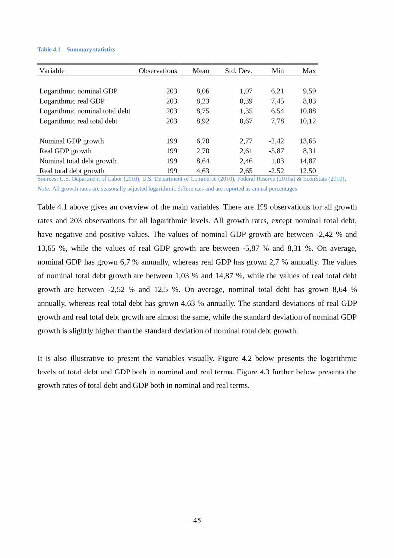
45
Table 4.1 – Summary statistics
Variable Observations Mean Std. Dev. Min Max
Logarithmic nominal GDP 203 8,06 1,07 6,21 9,59
Logarithmic real GDP 203 8,23 0,39 7,45 8,83
Logarithmic nominal total debt 203 8,75 1,35 6,54 10,88
Logarithmic real total debt 203 8,92 0,67 7,78 10,12
Nominal GDP growth 199 6,70 2,77 -2,42 13,65
Real GDP growth 199 2,70 2,61 -5,87 8,31
Nominal total debt growth 199 8,64 2,46 1,03 14,87
Real total debt growth 199 4,63 2,65 -2,52 12,50 Sources: U.S. Department of Labor (2010), U.S. Department of Commerce (2010), Federal Reserve (2010a) & EconStats (2010).
Note: All growth rates are seasonally adjusted logarithmic differences and are reported as annual percentages.
Table 4.1 above gives an overview of the main variables. There are 199 observations for all growth
rates and 203 observations for all logarithmic levels. All growth rates, except nominal total debt,
have negative and positive values. The values of nominal GDP growth are between -2,42 % and
13,65 %, while the values of real GDP growth are between -5,87 % and 8,31 %. On average,
nominal GDP has grown 6,7 % annually, whereas real GDP has grown 2,7 % annually. The values
of nominal total debt growth are between 1,03 % and 14,87 %, while the values of real total debt
growth are between -2,52 % and 12,5 %. On average, nominal total debt has grown 8,64 %
annually, whereas real total debt has grown 4,63 % annually. The standard deviations of real GDP
growth and real total debt growth are almost the same, while the standard deviation of nominal GDP
growth is slightly higher than the standard deviation of nominal total debt growth.
It is also illustrative to present the variables visually. Figure 4.2 below presents the logarithmic
levels of total debt and GDP both in nominal and real terms. Figure 4.3 further below presents the
growth rates of total debt and GDP both in nominal and real terms.

46
Panel (A): Nominal Panel (B): Real
Figure 4.2 – Logarithmic levels of total debt and GDP
Panel (A): Nominal Panel (B): Real
Figure 4.3 – Growth rates of total debt and GDP
Note: All growth rates are seasonally adjusted logarithmic differences.
4.3 Hypotheses
This section presents three hypotheses, which are motivated by the following questions. Does total
debt affect GDP? Does GDP affect total debt? If either one does, what are the effects? Can we say
anything about the causality?
The theoretical framework and related studies discussed in Chapter 3 might provide some answers.
However, these answers should also be tested empirically. According to the theoretical framework,

47
following hypotheses have been constructed:
Hypothesis 1: Contemporaneous and past total debt affects contemporaneous GDP. In other
words, the hypothesis suggests that GDP is endogenous. This is assumed to be due to
contemporaneous and past total debt might determine production, consumption and public
spending possibilities.
Hypothesis 2: Past GDP affects contemporaneous total debt. In other words, the hypothesis
suggests that total debt is endogenous. This is assumed to be due to the possibility that past
GDP might be used as collateral for debt creation.
Hypothesis 3: GDP growth responds differently to a shock in total debt growth depending on
the time horizon. High (low) total debt growth might increase (decrease) GDP in the near
future, but it might decrease (increase) GDP in the distant future. This is supposed to be due
to changes in purchasing power and inflexible prices. Total debt growth might increase
economic activity in the near future as more purchasing power is created than returned. In
contrast, total debt growth might decrease economic activity in the distant future as more
purchasing power is returned than created as debts mature. In addition, hoarding
(precautionary saving) might be more common during high level of debt.
The three hypotheses above will be empirically tested in the next chapter.

48
5 ECONOMETRIC ANALYSIS
This chapter presents the preliminary tests, the estimated regressions and the postestimation results.
First, however, some illustrative figures are presented and interpreted. Second, stationarity is tested.
Third, cointegration is tested. Fourth, the estimated regressions are presented. Fifth, Granger
causality is tested. Sixth, impulse response functions are visually presented. Finally, forecast error
variance decompositions are also visually presented. A detailed description of the applied
econometric methods can be found in Appendix A.
The present chapter examines the dynamic effects of total debt and GDP. The theory discussed in
Chapter 3 suggests studying the relation between debt and GDP. Previous studies, such as Sims
(1972), Moore (1989) and Bernanke (2000), use two-variable systems in order to explain the
interactions between money (or debt) aggregates and economic activity. In addition, Minsky (1982
& 1986) and Adrian and Shin (2009 & 2011) argue that instead of the money supply measures more
comprehensive credit aggregates should be analyzed. Moreover, any debt creation will most likely
be followed by a market transaction due to logical reasons. All these factors support the choice to
use two-variable structural VAR model in order to study the dynamic interactions of total debt and
GDP.
5.1 Total debt and GDP at a glance
This section examines the interrelations between total debt and GDP simply by presenting some
illustrative figures. The figures can also be helpful when determining the correct specification of the
model to be estimated. First, the contemporaneous effects are briefly examined. Then, we will move
to examine the dynamic effects.
A very rough way of examining the existence of a relationship between total debt and GDP is to
plot them against each other. Figure 5.1 shows the growth rates of total debt and GDP against each
other.

49
Panel (A): Nominal growth rates Panel (B): Real growth rates
Figure 5.1 – Scatterplots for total debt and GDP
Note: All variables are seasonally adjusted logarithmic differences.
As Figure 5.1 above depicts, there is a positive relation between the contemporaneous nominal and
real growth rates of total debt and GDP in the United States between 1959 and 2010. However, the
relation does not seem to be completely linear at least with the real growth rates. That is, even
though real total debt would grow faster, real GDP will not grow faster after a certain limit. The
limit seems to be approximately 8 % for both variables. This makes sense since real economy
clearly cannot grow arbitrarily fast and, thus, further real total debt growth would only stimulate
inflation instead of the real economy. On the other hand, negative real total debt growth can imply
deflation. Deflation, as has been discussed in Section 3.1, is known to be harmful for real economic
growth. Figure 5.1 Panel (B) shows that negative growth rates of real total debt are closely
associated with negative growth rates of real GDP.
There seems to be a positive contemporaneous correlation between the growth rates of total debt
and GDP, but it is even more important to study the dynamic effects. Figure 5.2 below presents the
time series of the real growth rates of total debt and GDP in the United States from 1959 to 2010.
As Figure 5.2 below confirms, real total debt and real GDP are clearly positively correlated. In other
words, real total debt is procyclical. As discussed in Chapter 3, creating new debt might increase
(decrease) GDP through new (lost) investment, consumption and public spending. The rate, at
which total debt is created (destroyed), is supposed to increase (decrease) as a consequence when
the central bank lowers (raises) the interest rate. However, an increase (decline) in GDP might also
enable more (less) debt creation as the collateral, against which debt is issued, increases (decreases).

50
Figure 5.2 – Real growth rates of total debt and GDP
Notes: Both variables are seasonally adjusted logarithmic differences and have been smoothed with
moving-average filter with four lags, one contemporaneous term and four forwards. The figure is
otherwise the same as Figure 4.3 Panel (B).
Interestingly, Figure 5.2 above depicts that real total debt has grown almost constantly faster than
real GDP after the year 1979, while before that they both grew approximately at the same rate. This
might be due to the new monetary policy procedures announced by the Federal Reserve in October
1979, which gave a start for an era of deregulation. This might also be deemed as Adrian and Shin’s
(2009 & 2011) turning point from bank-based credit to market-based credit.
The fact that real total debt has grown faster than real GDP might have some interesting
implications. It might imply that new purchasing power created by new total debt has mainly been
channeled to asset markets, instead of the real economy. This view is also supported by the fact that
asset prices, such as stock values, have grown notably faster than the real economy from 1979
onwards. If the new purchasing power would have been channeled solely to the real economy, the
total debt to GDP ratio could not have changed (unless the velocity of circulation changes), that is,
their growth rates should not depart from each other. Why? There are three explanations. First, if
new purchasing power would create real economic growth exactly in the same proportion, the ratio
could not change. Second, if new purchasing power would be only inflationary without any real
economic effects, the ratio could not change either as inflation is removed from the variables. Third,
logically a combination of these two effects should neither have any effects on the ratio. As the total
debt to GDP ratio has changed, as Figure 2.1 Panel (A) illustrated, we can relatively safely conclude
that new purchasing power created by an increase in total debt after 1979 has mainly been
channeled outside the real economy.

51
The structural break in 1979, however, should not go unnoticed in the regression analysis as it could
affect the estimates differently during these two periods. The existence of a structural break implies
two possible adjustments. Either a dummy-variable should be added from 1979Q4 onwards (or until
1979Q3). This might be the point when Adrian and Shin’s (2011, 65) “market-based financial
system” replaced its predecessor. Alternatively, two separate regressions could be estimated for pre-
and post-1979.
These procedures are commonly used in other empirical studies, where interactions between
quantity measures and economic activity are estimated. For instance, Friedman and Kuttner (1992)
use both methods. They adapt the third quarter of 1979 as a threshold for one subsample because
the Federal Reserve introduced its new monetary policy procedures in October 1979.
Next, we will take a brief outlook at the autocorrelations of the variables. Figure 5.3 presents the
autocorrelations of nominal variables, while Figure 5.4 presents the autocorrelations of real
variables.
Panel (A): Nominal GDP growth Panel (B): Nominal total debt growth
Figure 5.3 – Autocorrelations of nominal variables
Notes: Both variables are seasonally adjusted logarithmic differences. Bartlett's formula for MA(q) 95% confidence bands.
As Figure 5.3 above shows, both nominal variables are strongly and positively autocorrelated. The
first eleven lags of nominal GDP and the first nine lags of nominal total debt are statistically
significant. The autocorrelation of nominal GDP decays relatively rapidly to around 0,4 but
thereafter it is very persistent. The autocorrelation of nominal total debt, on the other hand, decays
very slowly and smoothly. Both variables seem to converge very slowly towards zero.

52
Panel (A): Real GDP growth Panel (B): Real total debt growth
Figure 5.4 – Autocorrelations of real variables
Notes: Both variables are seasonally adjusted logarithmic differences. Bartlett's formula for MA(q) 95% confidence bands.
According to Figure 5.4 above, also real variables are autocorrelated. However, only the first three
lags of real GDP and the first six lags of real total debt are statistically significant. Now, the
autocorrelation of real GDP decays notably fast to zero after five lags and then fluctuates around it.
The autocorrelation of real total debt decays more slowly reaching persistent negative values after
the tenth lag. Nevertheless, both variables tend to converge slowly towards zero.
Below in Figure 5.5 are shown cross-correlations between total debt growth and GDP growth. The
variables are both in nominal and real terms. Notice that total debt is on the horizontal axis
including lags and forwards, while GDP is on the vertical axis including only the contemporaneous
effects. Nevertheless, there is no reason to illustrate the variables with inverted axis because the
figure would simply be a mirror image (the cross-correlation of p-th lag of total debt with
contemporaneous GDP would be the same as the cross-correlation of p-th forward of GDP with
contemporaneous total debt).
According to nominal cross-correlations presented in Figure 5.5 Panel (A) below, there seems to be
a positive correlation between the nominal growth rates of GDP and total debt with all lags and
forwards. Correlation of the contemporaneous periods is the strongest correlation. The forwards of
total debt are also strongly correlated with GDP, while the lags are somewhat weaker correlated.

53
Panel (A): Nominal growth rates Panel (B): Real growth rates
Figure 5.5 – Cross-correlations of total debt and GDP
Notes: All variables are seasonally adjusted logarithmic differences. Total debt is on the horizontal axis (lags and forwards) and GDP
is on the vertical axis.
The argument that GDP is used as collateral for debt creation is supported by the fact that forwards
of total debt are strongly correlated with contemporaneous GDP. In addition, future GDP obviously
cannot be used as collateral, which could explain why lagged total debt is correlated weakly with
contemporaneous GDP. On the other hand, lagged total debt being weakly correlated with
contemporaneous GDP could indicate that past debt creation causing present GDP should be
questioned. However, the possibility that only the contemporaneous periods matter cannot be ruled
out. It is possible that contemporaneous total debt could cause contemporaneous GDP, even though
the lags of total debt do not have any effect on contemporaneous GDP.
When examining the real variables, as Figure 5.5 Panel (B) shows, the cross-correlations are
somewhat different. Still, the contemporaneous periods are most strongly and positively correlated.
Surprisingly, however, now the distant (more than 6 quarters) lags and forwards are negatively
correlated. Again the distant lags of real total debt are less correlated with contemporaneous real
GDP than distant forwards, but only slightly. The near (up to 6 quarters) lags and forwards are still
positively correlated. Now, however, the correlations of near lags and forwards are evenly
distributed, that is, the cross-correlations are not skewed. In addition, the cross-correlations of the
most distant lags and forwards tend to converge to zero.
The distant lags and forwards of real total debt being negatively correlated with contemporaneous
GDP raises some interesting questions. Could aggressive debt creation in the distant past affect
present GDP negatively? According to Figure 5.5 Panel (B), it might be possible. This makes sense

54
since, ceteris paribus, when past debts are repaid, more purchasing power is destroyed than created
(total debt is shrinking), which can affect contemporaneous real economic activity negatively if
prices are inflexible. Actually, this is analogous to the debt deflation theory, although the effect is
mitigated if new debt is issued in order to replace the repaid debts. This is also in line with King’s
(1994) observation that previous changes in private debt are negatively correlated with
contemporaneous changes in GDP in the 1990s recession. From this perspective, a higher (lower)
total debt growth rate could provide a higher (lower) GDP growth rate in the short run, but a lower
(higher) GDP growth rate in the intermediate run. The idea is captured by hypothesis 3, which was
already presented in Section 4.3.
What about future expectations? The interpretation of cross-correlations of the real variables is
consistent with the rational expectations theory (meaning that expectations will be realized in the
future). Thus, if a higher debt growth rate is expected in the near future, present real GDP increases.
The present real GDP is financed with increased present borrowing as the debt is easier to repay in
the future if there is going to be more borrowing in the future. In addition, it is reasonable to borrow
for investment or consumption if the interest rate is expected to drop soon (remember that the
central bank interest rate is assumed to influence the growth rate of total debt). However, if a lower
interest rate is expected to take place in the distant future, it is reasonable to wait and borrow later.
Consequently, the present GDP may be negatively affected. Again, it is possible to identify a
positive short-run relation, but a negative intermediate-run relation.
If we examine the most distant lags and forwards, the cross-correlations converge to zero.
Intuitively, it is easy to understand: very distant events in the past or future do not affect current
decision making. In other words, there are no long-run effects. Thus, the time horizon in the model
should be relevant. In the next section we will test the stationarity of the variables.
5.2 Stationarity tests
As Appendix A explains, a time-series analysis should begin with stationarity tests. Thus, this
section presents the results of the augmented Dickey-Fuller (ADF) tests. The tested variables are
logarithmic levels and growth rates (seasonally adjusted logarithmic differences) of total debt and
GDP both in nominal and real terms.

55
The variables were not tested in the level or difference form without first taking a natural logarithm
as they are clearly not stationary. In the level form both variables have an increasing mean and
variance in time and thus cannot be stationary. In the difference form both variables have a
relatively stable mean, but the variance is clearly increasing in time.
Table 5.1 below presents the ADF-tests for logarithmic levels and growth rates. The lag number for
every variable is determined using Akaike (AIC) and Bayesian (BIC) information criterion.
Table 5.1 – Augmented Dickey-Fuller tests
Variable Lags Test statistic Probability Stationary
Logarithmic nominal GDP 2 (BIC) -2,538 0,1064 No
Logarithmic nominal GDP 17 (AIC) -2,756 0,0648 Yes, P>90 %
Logarithmic nominal total debt 3 (BIC) -1,364 0,5992 No
Logarithmic nominal total debt 12 (AIC) -1,526 0,5206 No
Logarithmic real GDP 2 (BIC) -2,021 0,2773 No
Logarithmic real GDP 18 (AIC) -2,021 0,2773 No
Logarithmic real total debt 5 (BIC) -0,363 0,9162 No
Logarithmic real total debt 7 (AIC) -0,196 0,9390 No
Nominal GDP growth 13 (BIC) -1,084 0,7213 No
Nominal GDP growth 30 (AIC) -0,419 0,9069 No
Nominal total debt growth 9 (BIC) -1,349 0,6066 No
Nominal total debt growth 17 (AIC) -1,215 0,6670 No
Real GDP growth 14 (BIC) -3,468 0,0088 Yes, P>99 %
Real GDP growth 14 (AIC) -3,468 0,0088 Yes, P>99 %
Real total debt growth 9 (BIC) -3,412 0,0106 Yes, P>95 %
Real total debt growth 10 (AIC) -3,289 0,0154 Yes, P>95 % Notes: All growth rates are seasonally adjusted logarithmic differences. The information criterion supporting the lag choice is in the
parenthesis after the lag number. The ADF-test is conducted as a pure random walk model and thus does not include a drift term or a
linear time trend.
As Table 5.1 above shows, logarithmic GDP and total debt are nonstationary both in nominal and
real terms. This result should not come as a surprise as Figure 4.2 illustrates that the variables in
logarithmic levels clearly have an increasing mean in time, even though the variance seems
relatively stable. The only exception in logarithmic levels is the nominal GDP, when tested with 17
lags. In this case it is statistically significant at 10 % level, but not if it is tested with 2 lags. Hence,
using barely stationary logarithmic nominal GDP could be a risky and questionable choice.

56
Table 5.1 also shows that the nominal growth rates of the variables are not even remotely stationary.
This result is somewhat surprising as Figure 4.3 Panel (A) depicts that the mean wanders only
slightly across time and the variance is relatively stable. As Table 5.1 displays, the real growth rates
of the variables are, however, statistically significant at least at 5 % level. In other words, the real
growth rates of the variables are difference stationary I(1). Thus, it is reasonably safe to estimate the
model using real growth rates of total debt and GDP.
5.3 Cointegration tests
As concluded in the previous section above, the real growth rates of the variables are stationary.
Consequently, the variables cannot be straightforwardly estimated in the level form. Thus, the long-
run equilibrium13
between the variables cannot be studied, unless they are cointegrated. In the
present section cointegration of total debt and GDP is tested.
The economic logic behind the cointegration analysis is that economic variables do not typically
drift too far away from each other due to market mechanism or government intervention. This,
however, does not seem to be the case with the variables concerned in this study. As Figure 4.2
illustrated, it seems that real and nominal logarithmic levels of total debt and GDP have been
drifting apart practically the whole time period from 1959 to 2010. Thus, it seems unlikely that the
variables are cointegrated – at least in the time horizon examined in this study.
Nevertheless, the variables might be cointegrated in the very long run as, according to Morgan
Stanley (2009), the total debt to GDP ratio grew exponentially and reached 300 % in 1933, and
halved relatively fast in the next 10 odd years. As Figure 2.1 Panel (A) showed, the ratio climbed
again exponentially almost to 400 % until 2009, and thereafter it shows some signs of reaching a
turning point. Thus, it is possible that the total debt to GDP ratio will be dropping in the upcoming
years and, consequently, show some evidence of cointegration. Nevertheless, the potential
adjustment period is so long that it cannot be examined in this study.
As it seems unlikely that the variables would be cointegrated, we will settle to test for cointegration
13 It should be noted that econometricians typically have a different interpretation for the term equilibrium than
economists. These two interpretations should not be confused with each other. Here equilibrium simply refers to any
long-run relationship between non-stationary variables.

57
only with the Engle-Granger method and not apply Johansen method. The cointegration test results
using the Engle-Granger method are presented in Table 5.2 below.
Table 5.2 – Cointegration tests with Engle-Granger method
Variables Observations Lags Test statistic Cointegrated
Logarithmic nominal GDP & Logarithmic nominal total debt 199 3 (BIC) -0,695 No
Logarithmic nominal GDP &
Logarithmic nominal total debt 190 12 (AIC) -1,119 No
Logarithmic real GDP & Logarithmic real total debt 200 2 (BIC) -1,787 No
Logarithmic real GDP &
Logarithmic real total debt 199 3 (AIC) -1,867 No
Logarithmic real GDP & Logarithmic nominal total debt 200 2 (BIC) -2,637 No
Logarithmic real GDP &
Logarithmic nominal total debt 196 6 (AIC) -2,703 No Notes: Critical values for a sample size of 200 are: -3,067 for 10 %; -3,368 for 5 %; and -3,954 for 1 %. The information criterion
supporting the lag choice is in the parenthesis after the lag number.
As Table 5.2 above shows, none of the key variable pairs is cointegrated. The tested pairs are
nominal and real logarithmic levels of GDP and total debt. In addition, logarithmic real GDP is
tested with logarithmic nominal total debt. The finding is also supported by Figure 4.2 as nominal
and real logarithmic levels of total debt and GDP have been drifting apart practically the whole time
period from 1959 to 2010. Furthermore, Figure 2.1 Panel (A) shows that the total debt to GDP ratio
has been on an exponential trend path. When the variables are not cointegrated, the result indicates
that there is no long-run equilibrium. As the variables are not cointegrated but are difference
stationary I(1), the difference form of real variables should be used in estimation.
5.4 Estimated regressions
The estimated model is presented and the rationale behind it is explained in the present section. As
has been observed above, the key variables are difference stationary but not cointegrated. Thus, a

58
structural vector autoregressive (SVAR or structural VAR) model should be estimated in differenced
form for real total debt and real GDP.
In this study a structural VAR model is estimated using OLS. The model is the same as in equation
(4.9), or in a more compact form in equation (4.10). The estimated model presented already in
equation (4.9) is:
[𝑦𝑡𝑧𝑡] = [
𝑎10𝑎20
] + [𝑎11(1) 𝑎12(1)
𝑎21(1) 𝑎22(1)] [𝑦𝑡−1𝑧𝑡−1
] + (5.1)
+ [𝑎11(2) 𝑎12(2)
𝑎21(2) 𝑎22(2)] [𝑦𝑡−2𝑧𝑡−2
] + ⋯+ [𝑎11(𝑝) 𝑎12(𝑝)
𝑎21(𝑝) 𝑎22(𝑝)] [𝑦𝑡−𝑝𝑧𝑡−𝑝
] + [𝑒1𝑡𝑒2𝑡
]
where 𝑦𝑡 is seasonally adjusted logarithmic difference of real GDP, 𝑧𝑡 is seasonally adjusted
logarithmic difference of real total debt, and p is the number of lags. The number of lags is
determined with AIC and BIC, which suggest using 16 and 2 lags respectively.
As has been explained in Chapter 3, the contemporaneous causality runs from total debt to GDP.
The monetary circuit theory argues that debt creation is an important determinant of the production
process and hence must take place first. Thus, the variables have been ordered in this way and not in
the alternative way. In this ordering real total debt growth has a contemporaneous effect on real
GDP growth, but real GDP growth affects real total debt only with delay.
As explained in Section 5.1, due to the structural break in October 1979 the model is estimated
separately for the whole sample and two subsamples. The time horizon of the whole sample is
1959Q1–2010Q1, while the time horizons of the subsamples are 1959Q1–1979Q3 and 1979Q4–
2010Q1. In addition, the whole sample is estimated both with and without a dummy-variable for
1979Q4–2010Q1. These adjustments allow us to conduct also some comparative analysis.
The estimated model should be quite valid. The explanatory value of the whole sample with 16 lags
without the dummy-variable is very good. The R2-value of the real GDP growth equation is 0,90
and of the real total debt growth equation is 0,95. In addition, the error terms do not seem to be
autocorrelated as the Lagrange-multiplier test returns a high probability with almost all lag numbers
for the null hypothesis, which implies that there is no autocorrelation. Furthermore, there is 0,000 %
probability that all coefficients of either equation would be jointly zero.

59
5.5 Granger causality tests
The present section shows the results of Granger causality tests. Table 5.3 below presents the
probabilities of the null hypothesis for different model specifications. Rejecting the null hypothesis
implies that the the exluded variable contains predictive power over the lags of the dependent
variable and, thus, Granger causes the dependent variable.
Table 5.3 – Granger causality tests
Excluded variable Lags 1959Q1–2010Q1
(without dummy)
1959Q1–2010Q1
(with dummy)
1959Q1–1979Q3
1979Q4–2010Q1
Real total debt growth 2 (BIC) 0,087* 0,013** 0,032** 0,109
Real total debt growth 16 (AIC) 0,519 0,404 0,014** 0,004***
Real GDP growth 2 (BIC) 0,680 0,687 0,836 0,946
Real GDP growth 16 (AIC) 0,011** 0,019** 0,003*** 0,039** Notes: All variables are seasonally adjusted logarithmic differences. The dummy-variable is for 1979Q4–2010Q1. One asterisk
stands for 10 %, two asterisks for 5 % and three asterisks for 1 % significance level. The information criterion supporting the lag
choice is in the parenthesis after the lag number.
As Table 5.3 depicts, the results of Granger causality tests are somewhat ambiguous. In the whole
sample real total debt growth Granger causes real GDP growth at 10 % significance level when two
lags are used in estimation, but there is no Granger causality with 16 lags. Including the dummy-
variable for 1979Q4–2010Q1 increases the significance level at 5 % (almost at 1 %) with 2 lags, but
does not change the result of 16 lags.
Similar results are found with real GDP growth. Contrary to real total debt growth, however, real
GDP growth does not Granger cause real total debt growth with 2 lags, but it does Granger cause
real total debt growth with 16 lags at 5 % (almost at 1 %) significance level. Including the dummy-
variable hardly changes the results.
In the 1959Q1–1979Q3 subsample the findings are less ambiguous for real total debt growth. Now,
real total debt growth Granger causes real GDP growth at 5 % significance level with both 2 and 16
lags. The findings for real GDP growth are, however, quite contradictory. When the model is
estimated with 2 lags, real GDP growth does not Granger cause real total debt growth even

60
remotely, but with 16 lags it Granger causes real total debt growth even at 1 % significance level.
In the 1979Q4–2010Q1 subsample real total debt growth does not quite Granger cause real GDP
growth with 2 lags, but with 16 lags it does Granger cause real GDP growth even at 1 %
significance level. Also in this subsample real GDP growth does not Granger cause real total debt
growth even remotely with 2 lags, but with 16 lags it does Granger cause real total debt growth at 5
% significance level.
As has been pointed out above, Granger causality tests did not provide us with any straightforward
results. There is evidence to support but also to reject Granger causality between both variables in
all samples. The only exception is the 1959Q1–1979Q3 subsample, where real total debt growth
seems to Granger cause real GDP growth in both cases. In the next section the dynamic effects of
the variables will be examined in more detail. Finally, Section 5.7 provides us with further analysis
of the predictive power of the variables.
5.6 Impulse responses
This section presents the impulse response functions (IRF). First, impulse responses are visually
presented and analyzed. Then, the cumulative impulse responses are visually presented and
interpreted. Figure 5.6 below illustrates the orthogonalized impulse response functions.
Orthogonalized IRFs indicate that the error term is isolated and it does not keep on “bouncing” from
one IRF to another. In the orthogonalized IRFs the error terms are transformed so that the
covariance matrix of the error terms is an identity matrix. In other words, the errors are uncorrelated
and the variances (and standard deviations) of the error terms are one. Thus, one-unit (annual
percentages in this thesis) shock in the transformed error term is also one standard deviation shock.
Figure 5.6 below presents the impulse response functions to different shocks at 15 quarter forecast
horizon. As explained above, the shock is one annual percentage or one standard deviation. One of
the main findings is that all impulse responses are transitory. Furthermore, real GDP growth
responds positively to a real total debt growth shock. Real total debt growth, however, does not
respond to a real GDP growth shock. In addition, both variables respond positively to their own
shocks.

61
Figure 5.6 – Impulse response functions
Notes: All variables are seasonally adjusted logarithmic differences. The model is estimated using the whole sample with 16 lags and
without the dummy-variable.
The response of real GDP growth to a real total debt growth shock peaks approximately at 0,8 %
after three quarters, and then the response decays slowly to zero. The corresponding impact
multiplier, that is the contemporaneous effect, is approximately 0,4 %. These findings support
hypothesis 1 and the first part of hypothesis 3, but they reject the latter part of hypothesis 3. The
response of real total debt growth to a real GDP growth shock fluctuates around zero, and then the
response converges to slightly negative value, which is, however, not statistically significant. This
finding implies rejecting hypothesis 2. Due to the ordering of the variables, the corresponding
impact multiplier is necessarily zero.
The IRFs in Figure 5.6 are estimated using the whole sample with 16 lags and no dummy-variable.
To check for robustness the impulse responses were estimated also with alternative model
specifications. The alternative model specifications tell roughly the same story. Nevertheless, the
detailed results of IRFs using alternative model specifications are described below.

62
In the whole sample with 16 lags including the dummy-variable for 1979Q4–2010Q1 returns
practically identical results. Estimating the model with 2 lags smoothens the fluctuations, but
otherwise there are no differences. Also including the dummy-variable in the model with 2 lags
preserves the results unchanged.
The IRFs tell approximately the same story also for the two subsamples. The only noteworthy
difference is that the response of real GDP growth to real total debt growth is somewhat stronger,
compared to the whole sample, in the 1959Q1–1979Q3 subsample while the response is somewhat
weaker in the 1979Q4–2010Q1 subsample. Still the response of real total debt growth to a real GDP
growth shock does not depart from zero at any time.
The results are quite robust also with respect to alternative ordering of the variables. When
alternative ordering is adopted, there is a contemporaneous effect from real GDP to real total debt,
but not vice versa. In this case, the response of real GDP growth to a real total debt growth shock
peaks at 0,5 % after five quarters. Thus, the effect is slightly weaker, but it is still significantly
positive. Now, however, the response of real total debt growth to a real GDP growth shock is also
significant peaking at 0,6 % after 3 quarters, and then it decays to negative values although not
statistically significantly.
As has been observed above, all responses to various shocks are transitory. However, they are
transitory only when the growth rates are considered. It is possible that there are persistent level
effects. In order to obtain some view on the level effects we must study the cumulative effects of the
growth rates. Figure 5.7 below illustrates the cumulative orthogonalized IRFs.
Figure 5.7 presents the cumulative impulse response functions, in other words, the long-run
multipliers. The cumulative impulse response of real GDP growth to a real total debt growth shock
tends to converge to around 5 %. Also the cumulative impulse responses of real GDP growth and
real total debt growth to their own shocks converge to statistically significant positive values. The
cumulative impulse response of real total debt growth to a real GDP growth shock, however, does
not statistically significantly depart from zero even when the cumulative effects are examined.
Thus, it might be that the level effects tend to be persistent, although the effects of relative changes
seem to be only transitory.

63
Figure 5.7 – Cumulative impulse response functions
Notes: All variables are seasonally adjusted logarithmic differences. The model is estimated using the whole sample with 16 lags and
without the dummy-variable.
The overall effects of both shocks are as follows. One annual percentage shock to real total debt
growth might permanently increase its own level approximately by 7 % and the level of real GDP
by 5 %. One annual percentage shock to real GDP growth, on the other hand, might permanently
increase its own level approximately by 4 %, but it does not statistically significantly affect the
level of real total debt although it converges to negative values. Thus, the cumulative IRFs reinforce
the previous findings, which support hypothesis 1 and the first part of hypothesis 3 and reject
hypothesis 2 and the latter part of hypothesis 3.
As should be expected, the cumulative IRFs are also approximately similar when the model is
estimated with 2 lags and/or including the dummy-variable for 1979Q4–2010Q1. In the 1959Q1–
1979Q3 subsample the results are otherwise similar except with all four combinations the
cumulative responses tend to converge more strongly towards zero when the model is estimated
with 16 lags. However, such tendencies are not found in the model with 2 lags. In the 1979Q4–
2010Q1 subsample and 16 lags the results are similar than in the whole sample. However, in the

64
model with 2 lags the cumulative response of real GDP growth to real total debt growth shows signs
of deceleration but continuous growth, and the cumulative response of real total debt growth to its
own shock indicates over 10 % cumulative growth and slow deceleration.
5.7 Variance decompositions
This final section visually presents the results of forecast error variance decompositions (FEVD).
Figure 5.8 below presents the fractions of mean squared errors (MSE) due to different shocks.
Figure 5.8 – Forecast error variance decompositions
Notes: All variables are seasonally adjusted logarithmic differences. The model is estimated using the whole sample with 16 lags and
without the dummy-variable.
As Figure 5.8 above depicts, the shock of real total debt growth explains approximately half of the
real GDP growth forecast error variance at 15 quarter forecast horizon. Respectively, the shock of
real GDP growth explains approximately half of its own forecast error variance. This would imply
that real GDP growth is endogenous. The finding supports hypothesis 1. Contrastively, the shock of

65
real total debt growth explains all of its own forecast error variance and, respectively, the shock of
real GDP growth explains none of it. Hence, real total debt growth seems to be exogenous. This
finding suggests rejecting hypothesis 2.
The FEVDs in Figure 5.8 are estimated using the whole sample with 16 lags and no dummy-
variable. To check for robustness the FEVDs were estimated also with alternative model
specifications. The alternative model specifications return similar results. Nevertheless, the detailed
results of the FEVDs using alternative model specifications are described below.
The FEVDs are practically identical when the model is estimated using the whole sample with 2
lags and/or including the dummy-variable. In the 1959Q1–1979Q3 subsample the shock of real total
debt growth explains the forecast error variance of real GDP growth approximately 65 % at 15
quarter forecast horizon and, respectively, the shock of real GDP growth explains its own forecast
error variance only 35 %. When the subsample is estimated with 16 lags, the forecast error variance
of real total debt growth on a real GDP growth shock departs slightly from zero, but it is not
statistically significant. Respectively, the forecast error variance of real total debt growth on its own
shock departs slightly from 100 %, but not significantly. When the model is estimated with 2 lags,
there are no such departures. Thus, in the 1959Q1–1979Q3 subsample real GDP growth tends to be
slightly more endogenous and real total debt growth seems still exogenous.
In the 1979Q4–2010Q1 subsample and 16 lags the shock of real total debt growth explains the
forecast error variance of real GDP growth approximately 40 % at 15 quarter forecast horizon.
Respectively, the shock of real GDP growth explains 60 % of its own forecast error variance. With
only 2 lags the forecast error variances of real GDP growth are similar than in the whole sample.
The forecast error variances of real total debt growth are also very similar than in the whole sample
regardless whether 16 lags or only 2 lags are used in estimation. Hence, in the 1979Q4–2010Q1
subsample it seems that real GDP growth might be slightly less endogenous and real total debt
growth seems still entirely exogenous.

66
6 DISCUSSION
The present chapter discusses on the interpretation of the results and practical implications. First,
causality is discussed. Second, some contradictions between the findings and the theoretical
framework are discussed. Third, some policy suggestions are considered.
The most conservative way to interpret the results of this study is to state that contemporaneous and
past fluctuations in real total debt growth contain predictive power for contemporaneous real GDP
growth. In addition, past fluctuations in real GDP growth do not contain predictive power for
contemporaneous real total debt growth. If the statement is formulated in this fashion, it does not
necessarily refer to any causal relation between the variables. As Sims (1972) argues, it is possible
that there is no correspondence between causal ordering and temporal ordering. However, according
to Sims, few would deny any causal influence of money on economic activity and, on the other
hand, of economic activity on money.
This study, as does Sims (1972), takes a more courageous stance by interpreting the results also as
causal relations. Thus, contemporaneous and past fluctuations in real total debt growth cause
contemporaneous real GDP growth at least to certain extent, but there is no causal feedback from
past real GDP growth to contemporaneous real total debt growth.
On the other hand, endogenous money creation theory maintains that the demand for and supply of
debt are connected with the real economy. However, the causal interpretation does not imply that
the real economy does not have any influence on real total debt, even though only unidirectional
causality is found from real total debt to real GDP. The endogenous money creation theory argues
that the future expectations of economic development and the ability to repay debt dictate credit
arrangements, which influence the present observed economic development. This study argued that
observed real total debt influences observed real GDP. Thus, the causal and also temporal ordering
would be from expectations via debt to real economy.
In addition, expectations seem to be self-fulfilling. If expectations are positive, debt is demanded
and supplied, which causes the real economy to thrive. Following the same logic, thriving real
economy per se cannot be the proximate cause for past changes in debt. Instead, thriving real
economy can be one of the proximate causes for further positive expectations, which positively

67
influence the future demand and supply of debt, which then causes also the future economy to
thrive.
In principle, it is possible that real total debt is only correlated with some other factor, which is the
true cause for changes in real economic activity. Thus, real total debt would not have any true causal
relation to real economic activity. In this case, however, we should be able to hypothetically
manipulate the changes in real total debt and, ceteris paribus, it should not have any effect on real
GDP growth. Unfortunately, this obviously cannot be tested empirically. For instance, if solely
expectations would dictate the development of real GDP and expectations are positively correlated
with changes in real total debt, then manipulating the changes in real total debt while keeping the
expectations unchanged should not have any impact on real GDP. Nevertheless, this study maintains
that it would be quite implausible to argue that this kind of manipulation would not have any effect
on real economic activity as real total debt is most likely the proximate determinant of production,
consumption and public spending possibilities.
The findings of this thesis were mostly in line with the theoretical framework outlined previously.
The financial instability hypothesis and the monetary circuit theory suggested that money and debt
are main determinants of economic activity. The idea was included in hypothesis 1, which received
confirmation. An extension of the monetary circuit theory derived by the author of this thesis
suggested that the products of the real economy could be used as collateral for debt creation and,
thus, should have an effect on debt creation. This was included in hypothesis 2, but it was rejected.
The financial instability hypothesis and the monetary circuit theory also implied that economic
activity should be increased when debt increases. The first part of hypothesis 3 captured this and the
findings supported it. The latter part of hypothesis 3 combined debt deflation theory and monetary
circuit theory. The monetary circuit theory suggested that economic activity should decrease when
debts are repaid (without offsetting the effect with new issuance of debt), while the debt deflation
theory proposed that hoarding should increase during higher level of debt and that should decrease
economic activity. However, the findings did not support the latter part of hypothesis 3.
As has been explained above, hypothesis 2 and the latter part of hypothesis 3 were rejected.
Hypothesis 2 maintained that real GDP growth should have some effect on real total debt growth as
GDP might be used as collateral. It is possible that GDP is only a minor fraction of the available
collateral, while assets constitute the majority. Thus, the rejection of hypothesis 2 might be

68
explained with asset prices. The latter part of hypothesis 3 maintained that high (low) total debt
growth might decrease (increase) GDP in the distant future. Rejecting the latter part of hypothesis 3
might be explained with maturity distribution. As the maturity of debts is most likely not uniformly
distributed but instead scattered through time and it could also vary across time, the impulse
response analysis might not be able to identify a negative response in real GDP after the initial
positive response.
Although the findings were mostly consistent with the theoretical framework and previous
empirical studies outlined in Chapter 3, some differences could be observed. The findings seem to
stand in contrast also with Fisher’s debt deflation theory. Fisher (1933) argued that during the Great
Depression the nominal value of debt decreased, while the real value of debt increased. Thus,
changes in real debt should affect real economic activity in the opposite direction. This study,
however, found that changes in real total debt affect real economic activity in the same direction.
King (1994) might provide an explanation for this apparent discrepancy. He argued that decreasing
consumer prices are not a necessary condition for debt deflation. Instead, he argued that asset price
deflation is more important. Thus, if the definition of real total debt included also asset prices, it is
possible that the development of real total debt would be turned upside down and, hence, the
findings might be in line with Fisher (1933). For this reason it would be highly beneficial to
introduce also asset prices into the analysis. Moreover, in order to make a distinction between
changes in total debt due to price level changes and due to debt volume changes, price level could
be explicitly included into the analysis and total debt could be treated in nominal terms.
The present study found that real total debt is useful to predict real GDP also after 1979, while
Friedman and Kuttner (1992) found that neither money (measured with MB, M1 or M2) nor
domestic nonfinancial debt are useful to predict nominal or real GNP after 1979. The results of
these studies, however, do not necessarily contradict with each other. The different results might be
explained with different choices for the quantity variable. Adrian and Shin (2009 & 2011) as well as
Minsky (1982 & 1986) suggested using more comprehensive measures than money aggregates after
the market-based financial system replaced its predecessor. This replacement might be dated to
October 1979, when the Federal Reserve announced its new monetary policy procedures. As a
quantity variable this study applied total debt, which is notably more comprehensive than any
money supply measure or domestic nonfinancial debt examined by Friedman and Kuttner (1992).
Thus, the different results could be explained with the comprehensiveness of the financial quantity

69
variable: narrow measures have lost their significance, while broader measures have gained
importance.
Geanakoplos (2010), on the other hand, argued that increasing collateral rates were the proximate
cause for the present financial crisis. This study, however, put one piece in between. It is argued in
this thesis that increasing collateral rates decelerated real total debt growth, which was the
proximate cause for decelerating real GDP. Hence, this study tried to enrich Geanakoplos’s (2010)
analysis and should be seen as complementary.
There were also some similar limitations in this study and Geanakoplos’s (2010) approach. For
instance, Geanakoplos did not explicitly consider the level of debt – and neither did this study. If the
central bank pushed the collateral rates down, it might only balloon the real level of debt and, thus,
continue the “double bubble” of the housing market and the mortgage security market, or create a
new one in some other sector. Hence, regulating collateral rates could manage the crisis and have a
stabilizing effect, but it cannot solve the puzzle how the level of debt can be deleveraged if it is
already too high.
This study found that, particularly during a crisis, economic activity could be stimulated by
accumulating more debt. However, also this might only balloon the level of debt and, hence,
continue the “double bubble” or create a new one. Thus, neither the findings of this study can give
an explicit answer how to reduce the real level of debt if it is already too high. It is proposed that
debt-free money might offer one possibility to simultaneously reduce debt and support economic
growth. This proposition will be discussed later. First, however, other measures and their possible
consequences are discussed.
This study showed that achieving economic growth and total debt reduction simultaneously is
almost impossible. In other words, economic growth seems to require total debt growth. In Europe
there are strong demands to reduce public debt and at the same time to achieve economic growth. It
is, however, overly optimistic and unrealistic to imagine that economic growth will be achieved
while public debt is reduced or its growth rate is very slow. It could be possible if the private sector
would accumulate more debt. Yet, it is unlikely that the private sector will or can accumulate more
debt as it is already heavily indebted. In this case the level of total debt will be reduced, but
economic activity is most likely also severely damaged.

70
According to Fisher (1933) and Minsky (1982 & 1986), the “natural” way out of the crisis would be
through debt deflation and severe contraction in economic activity. As economic actors are unable
to service their debts, the aggregate supply will decrease through bankruptcies and other negative
events. Bankruptcies, by definition, decrease the amount of debt, but they might also increase the
price level. This could be deemed as supply-pull inflation or cost inflation. Increasing price level
also decreases the level of real debt. Ultimately, this kind of development will probably lead out of
the crisis, but, as Fisher (1933) argued, with devastating consequences.
Fisher (1933) argued that government intervention can always provide a more feasible way out of
the crisis. Private sector cannot have negative (monetary) net worth growth, at least for long, as it
would imply losses, bankruptcies, foreclosures etc. and it could lead to a debt deflation cycle. If the
public sector runs budget deficits – and consequently its net worth growth is negative – it will
necessarily increase the net worth of the private sector (given a balanced current account) as the
overall net worth is a zero-sum game. This would automatically enhance the repayment ability of
the private sector.
Consequently, it is suggested that measures to ensure real economic activity, while deleveraging
private debt, should be adopted. The public sector could accumulate more debt in order to support
economic growth and create (monetary) net worth for the private sector. In the long run, the
indebtedness of the private sector should be restored to a more reasonable level.
As the modern money theory implies, balancing the government budget is an absurd objective
during an economic recession. However, balancing the budget might be a justified goal within the
present financial institutions in the EMU as the member states are required to acquire funding
directly from the markets instead of the central bank. Within this framework a lower credit rating
could significantly deteriorate the possibilities of a government to acquire credit in the future. Thus,
within present financial institutions reasonable economic policy seems almost impossible, but
contractive economic policy seems also to have devastating consequences. As Wray (2000, 16)
aptly put it: “[b]y divorcing money from fiscal authority, the individual European nations will
probably have to retrench precisely when they should adopt expansionary policy.”
The United States can be seen as a financially sovereign country, which cannot drift into insolvency.
A financially sovereign country can borrow from the central bank and stimulate the economy by
increasing the level of public debt. However, in this situation the level of public debt is completely

71
ad hoc as the government can independently decide the amount of debt, the maturity of debt and the
interest rate of debt. The example of Japan has shown that the public debt to GDP ratio does not
matter as long as the financial sovereignty of the country is preserved. However, in Europe the
Maastricht Treaty – besides denying the member states acquiring funding directly from the ECB –
also limits the public debt of the member states to 60 % of their GDP. Thus, the EU countries are
not financially sovereign countries, but neither is the EU as a whole as it lacks independent fiscal
authority.
As the EU countries face restrictions set to their financial sovereignty, three alternative propositions
are put forward in order to reform the prevailing financial institutions. First, the EU countries could
be allowed to borrow directly from the ECB. This would enable them to stimulate the economy and
enhance the repayment ability of the private sector. Naturally, credit from the ECB should be
regulated as otherwise it could result in prisoner’s dilemma among the member states. Second, a
shared fiscal authority could be formed. The shared fiscal authority should be allowed to borrow
directly from the ECB and thus look after the solvency of all EU member states similarly as the
federal government of the United States looks after its states. Third, the euro could be abandoned
and the member states could return to their own national currencies. In this case the national
governments should be given the right to borrow directly from their national central banks.
Alternatively, a number of economists and economic commentators have suggested inflation as a
solution to the present financial crisis. As Fisher (1933) suggested, inflation would evaporate the
real level of debt and, therefore, it would reduce the total debt to GDP ratio. This seems to be a
reasonable suggestion, but causing demand-pull inflation in the present economic situation is very
difficult if not impossible without accumulating more debt. Demand-pull inflation is typically
observed when aggregate demand exceeds aggregate production capacity. However, as
unemployment rates are high and firms lay off workers it is clear that the aggregate production
capacity is not fully utilized. Thus, causing demand-pull inflation would require excessive
economic stimulus, which is normally achieved by accumulating debt.
If demand-pull inflation could be caused, commercial banks might grant excessive credit for asset
markets. In order to prevent a bubble, one possibility could be to raise the reserve and capital
requirements at least for funding asset acquisition. In addition, the government could grant credit
solely for real economic activities, increase spending and distribute income to low-end earners, who
have a higher marginal spending propensity on the real economy.

72
One more obstacle to cause demand-pull inflation is that, as Figure 2.1 Panel (B) showed, the public
sector has significantly shrunk compared to the private sector (measured with the amount of debt).
Thus, even aggressive economic stimulus by the government will not have a very significant effect
on the whole economy. As Minsky (1982 &1986) proposed, big government is needed in order to
have a significant impact on total debt through public debt and, thus, to stimulate the economy.
However, if the level of public debt or total debt has, for one reason or another, some limits,
alternative ways to stimulate the economy should be considered. One radical alternative could be to
inject debt-free money into the economy in order to simultaneously reduce the level of debt and
support economic growth. Debt-free money or Seignorage could also heal the fiscal deficit
problems and balance the government budget. Currently, Seignorage can be obtained mainly from
coins. Seignorage from coins is the difference between their nominal value and the production
costs. Seignorage from notes is only the avoided interest payments (minus production costs) as
notes are issued interest-free but not debt-free. Thus, as Kauko (2010) argues, printing notes
changes only the structure of debt, but not the amount. Seignorage from digital money would be the
nominal value itself as there would be practically no production costs. However, this kind of
Seignorage is not possible in the present monetary system.
Debt-free money could be created, for instance, via public spending to deleverage the total debt into
a more sustainable level. To give only one example, the long-run objective could be to create
enough debt-free money in order to keep the total debt to GDP ratio constant, as Fisher (1933)
proposed. The means are already available without any institutional changes as coins issued by the
government can be considered as debt-free money. This would simultaneously allow economic
stimulus and debt reduction. This would also enhance the financial position of both private and
public sectors. Inflation would not be a serious problem as it has been shown (e.g. McCandless and
Weber 1995) that inflation rate does not affect the rate of real economic growth with the exception
of hyperinflation and, of course, deflation. Ultimately, when the level of debt would be reduced
enough, the public sector could return to debt-based financing – if it is considered desirable.
According to Daly (1999, 133), one fundamental dilemma in the debt-based monetary system is that
in order to consume today’s production we must promise to produce even more tomorrow. That is,
as all money is debt, we necessarily need to carry some amount of debt in order to buy today’s
production. However, if debt bears positive real interest we must be able to produce even more

73
tomorrow in order to repay debt. Again, to buy tomorrow’s production we must promise to produce
even more the day after tomorrow etc. This is the reason why Daly (1999, 133) argues that the
present economic system creates artificial scarcity and, hence, is a “growth pusher” regardless of
the environmental constraints.
This thesis has only discussed how to stimulate economic growth. However, reducing economic
growth can be justified by, for example, ensuring environmental sustainability. In this case,
nonetheless, it would be reasonable to carefully control and plan the process, instead of
uncontrolled debt deflation, which might foster decisions that are unfavorable to the environment.
Also other and more efficient measures could be used than reducing the funding of welfare services
as they are likely to have only a very minor impact on environmental sustainability. Nevertheless,
economic growth has been a cross-party super ideology for long.
If ensuring environmental sustainability implies accepting negative economic growth, balancing
actions should be undertaken. For instance, income distribution policies should be practiced in order
to avoid social unrest. In addition, aggregate supply could be adjusted by reducing working hours.
This could avoid rising unemployment. Most likely various other actions should also be undertaken.
The measures described here should be taken only as first-step propositions.

74
7 CONCLUSIONS
This final chapter draws some conclusions. First, the research is summarized. Second, some
practical implications are considered. Third, limitations of the present study are discussed. Finally,
some suggestions for further research are given.
The main finding of this thesis was that changes in real total debt have effects on real economic
activity. The response of real GDP growth to a shock in real total debt growth seems to be
transitory, but the level effect might be persistent. In both cases the effect is in the same direction.
Thus, a positive shock in the growth rate of real total debt has a transitory positive effect on real
GDP growth rate, but may have a persistent positive effect on the level of real GDP. However, there
is no feedback from real economic activity to real total debt. The results reinforce some earlier
findings, provide practical advice and raise some new issues for further study.
7.1 Research summary
The purpose of this thesis was to study the dynamic effects of total debt and GDP. Total debt was
chosen because previous literature has mainly focused on money aggregates, public debt and other
less comprehensive quantity measures, while neglecting total debt. In addition, total debt to GDP
ratio has been on an exponential trend path in the United States ever since the 1970s and the ratio
reached record levels in the beginning of the present financial crisis. Furthermore, creation of any
debt will probably be followed by a market transaction due to logical reasons. These facts were
widely ignored by numerous leading economists.
The theoretical framework consisted of four distinct but related approaches. First, Minsky’s (1982
& 1986) financial instability hypothesis and Fisher’s (1933) debt deflation theory held that private
debt is a key factor influencing the real economy and the financial markets. They also maintained
that financial crises can be seen as a historical continuum. Second, the endogenous money creation
theory emphasized that commercial bank loans create deposits and also reserves are determined by
loans. In addition, the theory highlighted that the demand for money (and debt) originates from the
need of the real economy. Third, the modern money theory stressed that commercial banks can
create money, but payments between banks always have to be cleared solely with central bank
money. As currency derives its value from the government’s ability to levy taxes denominated in the

75
currency it issues, the main implication of the theory was that a financially sovereign country can
always clear its debt obligations and, thus, cannot drift into insolvency. Finally, the monetary circuit
theory described how production takes place from the perspective of money and debt. It held that
the role of money is to enable the circulation of commodities, but money and debt also determine
the level of production and consumption.
The method of this study was a time-series regression analysis, in which a two-variable structural
VAR model was estimated. The dynamic interactions between real total debt growth and real GDP
growth were studied with Granger causality tests, impulse response functions and forecast error
variance decompositions. The data was based on the United States from 1959 until 2010 and it was
organized quarterly.
The following hypotheses were formed based on the theoretical framework:
Hypothesis 1: Contemporaneous and past total debt affects contemporaneous GDP. In other
words, the hypothesis suggests that GDP is endogenous. This was assumed to be due to
contemporaneous and past total debt might determine production, consumption and public
spending possibilities.
Hypothesis 2: Past GDP affects contemporaneous total debt. In other words, the hypothesis
suggests that total debt is endogenous. This was assumed to be due to the possibility that
past GDP might be used as collateral for debt creation.
Hypothesis 3: GDP growth responds differently to a shock in total debt growth depending on
the time horizon. High (low) total debt growth might increase (decrease) GDP in the near
future, but it might decrease (increase) GDP in the distant future. This was supposed to be
due to changes in purchasing power and inflexible prices. Total debt growth might increase
economic activity in the near future as more purchasing power is created than returned. In
contrast, total debt growth might decrease economic activity in the distant future as more
purchasing power is returned than created as debts mature. In addition, hoarding
(precautionary saving) might be more common during high level of debt.
The main findings of this study showed that contemporaneous and past real total debt growth seems
to affect contemporaneous real GDP growth. The response of real GDP growth to a shock in real
total debt growth seems to be transitory as the corresponding impulse response function converges
to zero. However, the level effect might be persistent as the corresponding cumulative impulse
response function converges to a statistically significant positive value. In both cases the effect is in

76
the same direction. Thus, a positive shock in the growth rate of real total debt tends to have a
transitory positive effect on real GDP growth rate, but possibly a persistent positive effect on the
level of real GDP. Nevertheless, there seems to be no feedback from past real GDP growth to
contemporaneous real total debt growth as impulse responses and variance decompositions are not
statistically significant.
The main findings of this study supported hypothesis 1, but rejected hypothesis 2. The findings
implied that real GDP growth is endogenous, but real total debt growth is exogenous. The findings
of Granger causality tests were somewhat ambiguous. They were unable to discriminate between
the possibility for bidirectional causality, unidirectional causality running to either way or absence
of any causal relation. On the other hand, the results of impulse responses and variance
decompositions were quite unambiguous. They all supported unidirectional causality running from
real total debt to real GDP.
The findings of this study supported the first part of hypothesis 3, which stated that a shock in real
total debt growth affects real GDP growth in the same direction in the near future. However, the
latter part of hypothesis 3 did not receive significant support. Although a shock in real total debt
growth affects real GDP growth slightly in the opposite direction in the distant future, the response
is not statistically significant.
Although the findings were mostly consistent with the theoretical framework and previous
empirical studies, some differences could be observed. The findings seemed to stand in contrast also
with Fisher’s debt deflation theory. According to Fisher (1933), changes in real debt should affect
real economic activity in the opposite direction. This study, however, found that changes in real
total debt affect real economic activity in the same direction.
King (1994) might provide an explanation for this apparent discrepancy. He argued that decreasing
consumer prices are not a necessary condition for debt deflation, but, instead, asset price deflation is
more important. Thus, if asset prices would be included into the analysis, it is possible that the
findings would be in line with Fisher (1933).
The present study strengthened the previous findings of Sims (1972). He found that in a two-
variable model GNP is endogenous, while money measured with MB or M1 is exogenous. This
thesis found very similar results, although GNP was replaced with real GDP and money was
77
replaced with real total debt. In addition, this study shared the view of Sims that the relation is truly
causal.
On the other hand, Friedman and Kuttner (1992) found that neither money (measured with MB, M1
or M2) nor domestic nonfinancial debt are useful to predict nominal or real GNP after 1979, while
before that they contained significant predictive power. The present study adopted similar
subsampling and found that real total debt is useful to predict real GDP also after 1979.
The results of these studies, however, do not necessarily contradict with each other. The different
results might be explained with different choices for the financial quantity variable. Adrian and Shin
(2009 & 2011) as well as Minsky (1982 & 1986) suggested using more comprehensive measures
than money aggregates. As a quantity variable this study chose real total debt, which is notably
more comprehensive than any money supply measure or domestic nonfinancial debt examined by
Friedman and Kuttner (1992). Thus, the different results could be explained with the
comprehensiveness of the quantity variable: narrow financial measures have lost their significance,
while broader financial measures have become more significant.
7.2 Practical implications
The results of this study indicated that an increase in real total debt might increase permanently
aggregate economic activity measured with real GDP. Similarly, a decrease in real total debt might
imply a permanent decrease in real GDP. Thus, total debt seems to dictate, at least to some extent,
aggregate economic activity.
Hence, economic growth and total debt reduction seems to be almost an impossible combination.
Especially in Europe there are strong demands to reduce public debt, while at the same time
economic activity should be stimulated. If the private sector would be willing to accumulate more
debt, this result might be possible to achieve. Yet, more likely the private sector is unwilling or
unable to accumulate more debt as it is already heavily indebted. In addition, cutting public
expenditures will probably make the future look even more uncertain and it could also weaken the
repayment ability of the private sector. Thus, during public expenditure cuts it is even more
probable that the private sector is going to reduce rather than accumulate debt. In the present
situation, reducing public debt will almost certainly imply reduction in total debt and, hence,

78
reduction in economic activity.
As Fisher (1933) and Minsky (1982 & 1986) argued, the “natural” way out of the crisis would be
through debt deflation and radical decline in output. As economic actors are unable to service their
debts, the aggregate supply will decrease through bankruptcies and other negative events.
Bankruptcies, by definition, decrease the amount of debt, but they might also increase the price
level. This could be deemed as supply-pull inflation or cost inflation. Increasing price level
evaporates the level of real debt. Ultimately, this kind of development will probably lead out of the
crisis, but, as Fisher (1933) argued, with devastating consequences.
According to Fisher (1933), government intervention might provide a more reasonable way out of
the crisis. If the private sector will not or cannot accumulate more debt, the public sector should
take the lead. If public expenditures would increase, some proportion of it would, of course, end up
to the private sector and, thus, increase its (monetary) net worth. Higher net worth automatically
increases the repayment ability of the private sector and might encourage it to accumulate more
debt.
As has been argued previously, a financially sovereign country cannot drift into insolvency. The
United States can be considered as a financially sovereign country, although it has set a debt ceiling
to itself. In Europe, however, the Maastricht Treaty limits the public debt of the EU countries to 60
% of their GDP and denies borrowing directly from the ECB. Thus, the EU countries are not
financially sovereign countries and neither is the EU as a whole as it has no independent fiscal
authority. In the present situation the EU countries should be allowed to borrow directly from the
ECB. This would enable them to stimulate the economy and enhance the repayment ability of the
private sector. Another option for Europe would be to form a shared fiscal authority, which could
borrow directly from the ECB and thus look after the solvency of all EU member states. Third
option would be to abandon the euro and return to national currencies. In this case the national
governments should be given the right to borrow from their national central banks.
Alternatively, the repayment ability of the private sector could be enhanced by demand-pull
inflation in order to decrease the real value of private debt. However, as long as the full production
capacity of the economy is not utilized and unemployment exists (apart from frictional
unemployment), demand-pull inflation is hard to achieve. Hence, causing demand-pull inflation
would probably involve even stronger public stimulus than the measures described above.

79
However, if the level of public debt or total debt has, for one reason or another, some limits,
alternative ways to inject purchasing power into the economy should be considered. One radical
alternative could be to inject debt-free money into the economy, for instance, via public spending to
deleverage the total debt into a more sustainable level. The means are already available without any
institutional changes, namely, coins issued by the government can be considered as debt-free
money. This would allow both economic stimulus and debt reduction. This would also enhance the
financial position of both private and public sectors.
This thesis has only considered how to stimulate economic activity. Ensuring environmental
sustainability, however, could imply accepting negative economic growth. Nevertheless, in this case
it would be reasonable to closely control the process instead of uncontrolled debt deflation, which
might foster decisions that are unfavorable to the environment. If negative economic growth is
necessary, balancing actions should be undertaken. For instance, income distribution policies should
be practiced in order to avoid social unrest. In addition, working hours could be reduced in order to
adjust aggregate supply and avoid rising unemployment. Most likely a number of other actions
should also be undertaken, but the actions described here should be taken as first-step suggestions.
7.3 Limitations of the study
As every study, the present study has also some limitations. First of all, this study examined only
one country – the United States. The dynamic effects of real total debt and real GDP could vary
between countries and, thus, the generalisability of the results might be questioned.
This study considered only the growth rate effects, but not the level effects. Thus, the study focused
on short-run dynamics, but it could not say anything about the long-run equilibrium between the
variables. The level effects cannot be directly studied as the variables are in this form neither
stationary nor cointegrated. Nevertheless, this study examined the level effects indirectly with
cumulative impulse response functions.
The present study did not examine supply and demand factors in detail but only the observed
values. The demand for and supply of debt are probably mainly affected by future prospects
(including current indebtedness) to service and repay debt. This thesis, however, focused on

80
observed debt and its interaction with observed GDP. Further analysis of demand and supply of debt
lay beyond the scope of this paper.
This study did not examine what causes the shocks to total debt and GDP, but only the potential
effects of the shocks on these variables. Shocks to total debt might come from, for instance, changes
in interest rate, collateral rate or future prospects. Shocks to GDP might come from a number of
factors. This study, however, did not focus on different explanations for shocks. Instead, this study
focused on the interactions among the variables caused by the shocks. Thus, explaining the causes
of the shocks was mainly left for other researchers.
It is possible that also other factors influence real GDP and real total debt. This study, however,
considered only these two factors. Asset values were excluded, but they could have a significant
impact on debt creation and debt deflation. One explanation why the results of the regression
analysis might not always apply is that the proportion of total debt channeled to different purposes
has varied also within the subsamples. Thus, high total debt growth before the financial crisis may
have mainly influenced asset values, which indeed have developed quite favorably. Similarly,
during the financial crisis and lower total debt growth asset values have plummeted, while real GDP
has not reacted as strongly, although the direction has been the same to certain extent.
Neither was the price level explicitly included into the analysis. Thus, the study cannot discriminate
whether changes in real total debt are due to changes in the price level or changes in the volume of
debt. It is possible that that real GDP reacts differently to price level changes than to changes in the
nominal amount of total debt.
In this study it was assumed that marginal spending propensity out of total debt on the real economy
has been constant in the whole sample or at least within the subsamples. In other words, the
proportion of new total debt spent between the real economy and other purposes, such as asset
markets and hoarding, was assumed to be constant. However, the proportion may have permanently
changed in 1979. In the present thesis this was taken into account with the dummy-variable and
splitting the whole sample into two subsamples. Nevertheless, the proportion may have changed
also within the subsamples, which might reduce the explanatory power of the results.
As was discussed in Section 4.2, external debt (domestic debt borrowed from foreign entities)
should be excluded from the analysis as it probably mainly affects imports, which are not a part of

81
GDP. This study, however, did not make a distinction whether debt is borrowed from domestic or
foreign entities. Nevertheless, excluding external debt from the analysis might not be necessary if
its share of total debt stayed constant over the whole sample or at least within the subsamples.
Consequently, it would not have any effects on the growth rate of total debt and, therefore, does not
affect the results. Also if external debt is a very minor share of total debt, it should not have any
significant effect on the results.
It is possible that no cointegration vector could be estimated between the variables, even if the
variables were cointegrated. The adjustment period would probably be too long as the last turning
point in the total debt to GDP ratio was reached during the Great Depression. As a clear turning
point is reached very seldom, there is not enough repeatability to forecast it statistically.
In addition, the estimated coefficients could vary depending on the leverage phase. In other words,
the model might have a good predictive power when total debt is accumulated, but does not
necessarily have a very good predictive power when total debt is reduced. Unfortunately, the current
financial crisis is so recent that it is difficult to estimate separate regressions for these two time
periods. Moreover, there is no counterfactual available. Thus, it cannot be observed what would
have happened if the total debt of the United States did not increase as much as it has done.
Finally, this study was not able to precisely identify potential negative shocks to GDP caused by
previous increases in debt. In order to study the effects of debt repayment the maturity of debt
should be rather uniformly distributed. Thus, if a positive debt shock occurred at period 𝑡 = 0, a
corresponding negative shock to GDP should realize when the debt is repaid after period 𝑡 = 0 + 𝑥,
where 𝑥 is a positive constant. This is a problematic assumption as the maturity is more likely to be
scattered across multiple quarters and may even vary over time. This might be one explanation why
the impulse response analysis cannot identify a negative real GDP response after the initial positive
response. Although the subsequent values of real GDP growth are negative, they are not statistically
significant.
7.4 Suggestions for further research
The present study suggests at least seven directions for further research. First, as asset values are an
important factor influencing debt creation and debt deflation, asset prices (e.g. stock price index or

82
housing price index) could be introduced into the model. Thus, a three-variable model could be
estimated for real total debt, real GDP and asset prices. Alternatively, nominal total debt could be
used instead and consumer price level could be explicitly included into the model as a fourth
variable. This could also yield results with more practical significance as nominal debt can be
influenced more straightforwardly. However, nominal total debt seems to be non-stationary and,
hence, it should somehow be converted into a stationary time series.
Second, this study considered only the United States. In order to enhance generalisability and
comparability the same model could be estimated for other countries. Also panel data, that is
including multiple countries in the estimation, could be utilized.
Third, external debt (domestic debt borrowed from foreign entities) could be excluded from the
analysis. The reason behind this is that it probably mainly affects imports, which are not a part of
GDP.
Fourth, total debt could be decomposed into public and private debt in order to analyze their
potential different impacts. Total debt could also be decomposed alternatively, for example, into
public, household, business, financial and foreign debt.
Fifth, if enough data is available, the model could be estimated for pre-crisis (debt leveraged) and
post-crisis (debt deleveraged) periods separately. It is possible that the effects differ depending on
the time period.
Sixth, if the economy adjusts to growth rates of the variables, the model could be estimated for
seasonally adjusted second differences to study the effects of changes in growth rates. Finally,
different methodology could be used to explain the turning points in the total debt to GDP ratio.

83
REFERENCES
Adrian, Tobias & Moench, Emanuel & Shin, Hyun Song 2010. Macro Risk Premium and
Intermediary Balance Sheet Quantities. IMF Economic Review 58, 179-207.
Adrian, Tobias & Shin, Hyun Song 2011. Financial Intermediaries and Monetary Economics.
Published in Friedman, Benjamin & Woodford, Michael (eds.) Handbook of Monetary Economics.
Amsterdam: Elsevier. 601-650.
Adrian, Tobias & Shin, Hyun Song 2010. Liquidity and Leverage. Journal of Financial
Intermediation 19 (3), 418-437.
Adrian, Tobias & Shin, Hyun Song 2009. Money, Liquidity and Monetary Policy. Federal Reserve
Bank of New York Staff Reports No. 360.
Ahokas, Jussi & Holappa, Lauri 2010. Accumulation without Production. Paper presented at the
Coimbra Conference between 21th and 23
th of October.
Ahokas, Jussi & Kannas, Olli 2009. Finanssikriisin taustalla yksityisen velan määrän
räjähdysmäinen kasvu. Kansantaloudellinen aikakauskirja 105 (2), 186-201.
Auvinen, Tero 2010. On Money. University of Lapland, Doctoral Dissertation. Rovaniemi: Lapin
Yliopistokustannus.
Bank of Finland 2011. The Financial System in Brief. Available at:
http://www.suomenpankki.fi/en/rahoitusjarjestelman_vakaus/lyhyesti/Pages/default.aspx
Bernanke, Ben 2002. Deflation: Making Sure ”It” Doesn’t Happen Here. Speech held before the
National Economist Club, Washington D.C at 21.11.2002.
Bernanke, Ben 2000. Essays on the Great Depression. Princeton, New Jersey: Princeton University
Press.

84
Bloomberg 2011a. Greece Govt Bond 10 Year Acting as Benchmark. Available at:
http://www.bloomberg.com/apps/quote?ticker=GGGB10YR:IND
Bloomberg 2011b. Japan Govt Bond Year to Maturity 10 Year Simple Yield. Available at:
http://www.bloomberg.com/apps/quote?ticker=GJGB10:IND
Bloomberg 2011c. US Generic Govt 10 Year Yield. Available at:
http://www.bloomberg.com/apps/quote?ticker=USGG10YR:IND
Daly, Herman 1999. Ecological Economics and the Ecology of Economics: Essays in Criticism.
Cheltenham: Edward Elgar.
Dickey, David & Fuller, Wayne 1979. Distribution of the Estimates for Autoregressive Time Series
with a Unit Root. Journal of the American Real Estate and Urban Economics Association 20 (1),
181-197.
Disyatat, Piti 2008. Monetary Policy Implementation: Misconceptions and their Consequences. BIS
Working Papers No 269.
EconStats 2010. Debt Outstanding by Sector.
Enders, Walter 2004. Applied Econometric Time Series. Second edition. New York, NY: John Wiley
& Sons.
Engle, Robert & Granger, Clive 1987. Cointegration and Error-Correction: Representation,
Estimation, and Testing. Econometrica 55, 251-276.
Fama, Eugene 1970. Efficient Capital Markets: A Review of Theory and Empirical Work. Journal
of Finance 25, 383-417.
Fama, Eugene 1965. The Behavior of Stock Market Prices. Journal of Business 38, 34-105.
Febrero, Eladio 2009. Three Difficulties with Neo-Chartalism. Journal of Post Keynesian
Economics 31 (3), 523-541.

85
Febrero, Eladio 2006. Monetary Theory of Production: A Classical-Circuitist Alternative
Interpretation. Paper presented at X Jornadas de Economía Crítica in Barcelona between 23th
and
25th of May.
Federal Reserve 2010a. Flow of Funds Accounts of the United States.
Federal Reserve 2010b. Money Stock Measures.
Fisher, Irving 1933. The Debt-Deflation Theory of Great Depressions. Econometrica 1, 337-357.
Fisher, Irving 1930. The Theory of Interest. New York, NY: Macmillan.
Friedman, Benjamin 1981. Debt and Economic Activity in the United States. National Bureau of
Economic Research Working Paper No. 704.
Friedman, Benjamin & Kuttner, Kenneth 1992. Money, Income, Prices, and Interest Rates.
American Economic Review 82 (3), 472-492.
Geanakoplos, John 2010. Managing the Leverage Cycle: A Brief Talk in Milan with Questions and
Answers. Cowles Foundation Paper No. 1306.
Granger, Clive & Newbold, Paul 1974. Spurious Regression in Econometrics. Journal of
Econometrics 2, 111-120.
Graziani, Augusto 2003. The Monetary Theory of Production. Cambridge, MA: Cambridge
University Press.
Graziani, Augusto 1989. The Theory of the Monetary Circuit. Thames Papers in Political Economy,
Spring, 1-26.
Hahn, Frank 1966. Equilibrium Dynamics with Heterogeneous Capital Goods. Quarterly Journal of
Economics 80, 633-646.

86
Hannsgen, Greg 2005. Minsky's Acceleration Channel and the Role of Money. Journal of Post
Keynesian Economics 27 (3), 471-489.
IMF 2011. World Economic Outlook Database. Available at:
http://www.imf.org/external/pubs/ft/weo/2011/01/weodata/index.aspx
Innes, Mitchell 1913. What is Money? Banking Law Journal, May, 377-408.
Kauko, Karlo 2010. Velaton raha? Email interview between 20th and 22
th October.
Keen, Steve 2009. The Dynamics of the Monetary Circuit. Published in The Political Economy of
Monetary Circuits: Tradition and Change in Post-Keynesian Economics edited by Ponsot, Jean-
Francois & Rossi, Sergio. Basingstoke, UK: Palgrave. 161-187.
Keen, Steve 2001. Debunking Economics: The Naked Emperor of Social Sciences. London/New
York: Zed Books.
Keen, Steve 1995. Finance and Economic Breakdown: Modeling Minsky's Financial Instability
Hypothesis. Journal of Post Keynesian Economics 17, 607-635.
Keynes, John Maynard 1973. The Collected Writings of John Maynard Keynes VII. London:
Macmillan.
Keynes, John Maynard 1971 [1930]. A Treatise on Money. London: Macmillan.
Keynes, John Maynard 1936. The General Theory of Employment, Interest and Money. London:
Macmillan.
King, Mervyn 1994. Debt Deflation: Theory and Evidence. European Economic Review 38 (3-4),
419-445.
Korhonen, Tapio 2007. Raha ja luotto rahapolitiikassa. BoF Online 3. Available at:
http://www.suomenpankki.fi/fi/julkaisut/selvitykset_ja_raportit/bof_online/Documents/BoF_Online
_3_2007_Korhonen.pdf

87
Knapp, Georg 1924. The State Theory of Money. The first German edition was published in 1905.
London: Macmillan.
Krugman, Paul & Eggertsson, Gauti 2011. Debt, Deleveraging, and the Liquidity Trap: A Fisher-
Minsky-Koo approach. Unpublished second draft.
Krugman, Paul & Wells, Robin 2009. Macroeconomics. Second edition. New York, NY: Worth
Publishers.
Krugman, Paul & Wells, Robin 2006. Economics. New York, NY: Worth Publishers.
Kydland, Finn & Prescott, Edward 1990. Business Cycles: Real Facts and a Monetary Myth.
Federal Reserve Bank of Minneapolis Quarterly Review 14 (2), 3–18.
Lavoie, Marc 2003. A Primer on Endogenous Credit-Money. Published in Studies in the Modern
Theories of Money edited by Rochon, Louis-Philippe & Rossi, Sergio. Cheltenham: Edward Elgar.
506-543.
Lavoie, Marc 1987. Monnaie et production: Une synthèse de la théorie du circuit. Economies et
Sociétés, Série Monnaie et Production 4, 65-102.
Lerner, Abba 1947. Money as a Creature of the State. American Economic Review 37 (2), 312-317.
Lucas, Robert 2003. Macroeconomic Priorities. Speech held at the Presidential Address to the
American Economic Association at 10.1.2003.
McCandless, George & Weber, Warren 1995. Some Monetary Facts. Federal Reserve Bank of
Minneapolis Quarterly Review 19 (3), 2-11.
Minsky, Hyman 1986. Stabilizing an Unstable Economy. New Haven, Connecticut: Yale University
Press.
Minsky, Hyman 1982. Inflation, Recession and Economic Policy. Sussex: Wheatsheaf.
88
Moore, Basil 1989. The Endogeneity of Credit Money. Review of Political Economy 1 (1), 65-94.
Moore, Basil 1988. Horizontalists and Verticalists: The Macroeconomics of Credit Money.
Cambridge, MA: Cambridge University Press.
Morgan Stanley 2009. Economy + Internet Trends. Available at:
http://www.morganstanley.com/institutional/techresearch/pdfs/MS_Economy_Internet_Trends_102
009_FINAL.pdf
Nasica, Eric & Raybaut, Alain 2005. Profits, Confidence and Public Deficits: Modeling Minsky's
Institutional Dynamics. Journal of Post Keynesian Economics 28 (1), 136-154.
Nersisyan, Yeva & Wray, Randall 2010. Does Excessive Sovereign Debt Really Hurt Growth? A
Critique of This Time is Different, by Reinhart and Rogoff. Levy Economics Institute Working
Paper No. 603.
Parquez, Alain 1984. La Dynamique de la Monnaie. Economies et Sociétés, Série Monnaie et
Production 1, 83-118.
Pekkarinen, Jukka 1995. Keynes ja velkadeflaatio. Labour Institute for Economic Research
Discussion Paper No. 124.
Pollins, Robert 1991. Two Theories of Money Supply Endogeneity: Some Empirical Evidence.
Journal of Post Keynesian Economics 13 (3), 366-397.
Reinhart, Carmen & Rogoff, Kenneth 2010. Growth in a Time of Debt. American Economic Review
100 (2), 573-78.
Reinhart, Carmen & Rogoff, Kenneth 2009. This Time Is Different: Eight Centuries of Financial
Folly. Princeton, New Jersey: Princeton University Press.
Rochon, Louis-Philippe 1999. The Creation and Circulation of Endogenous Money: A Circuit
Dynamique Approach. Journal of Economic Issues 33 (1), 1-21.

89
Roubini, Nouriel & Setser, Brad 2005. Will the Bretton Woods 2 Regime Unravel Soon? The Risk
of Hard Landing in 2005-2006. Paper presented at the Symposium on the Revived Bretton Woods
System: A New Paradigm for Asian Development? in San Francisco at 4th of February.
Samuelson, Paul 1967. Indeterminacy of Development in a Heterogeneous Capital Model with
Constant Saving Propensity. Published in Shell, K. (ed.) Essays on the Theory of Optimal Economic
Growth, 219-232. Cambridge, MA: MIT Press.
Samuelson, Paul & Nordhaus, William 2009. Economics. Nineteenth edition. New York, NY:
McGraw-Hill.
Sargent, Thomas & Wallace, Neil 1981. Some Unpleasant Monetarist Arithmetic. Federal Reserve
Bank of Minneapolis Quarterly Review 5, 1-18.
Schumpeter, Joseph 1911. The Theory of Economic Development: An Inquiry into Profits, Capital,
Credit, Interest and the Business Cycle. Translated in 1934. Cambridge, MA: Harvard University
Press.
Shanmugam, Bala & Nair, Mahendhiran & Li, Ong Wee 2003. The Endogenous Money Hypothesis:
Empirical Evidence from Malaysia (1985-2000). Journal of Post Keynesian Economics 25 (4), 599-
611.
Sims, Cristopher 1972. Money, Income, and Causality. American Economic Review 62 (4), 540-
552.
Sloman, John 2006. Economics. Sixth edition. Harlow: FT Prentice Hall.
Stiglitz, Joseph 1990. Symposium on Bubbles. Journal of Economic Perspectives 4 (2), 13-18.
Tarvonen, Mikko 2011. Endogenous Money Creation in the European Monetary Union. University
of the Thai Chamber of Commerce, Master’s Thesis.
Tobin, James 1980. Asset Accumulation and Economic Activity. Oxford: Basil Blackwell.
90
U.S. Department of Labor 2010. Consumer Price Index: All Urban Consumers (CPI-U).
U.S. Department of Commerce 2010. National Economic Accounts.
Vera, Alfonso 2001. The Endogenous Money Hypothesis: Some Evidence from Spain (1987-1998).
Journal of Post Keynesian Economics 23 (3), 509-527.
Wicksell, Knut 1898. Interest and Prices. Translated by Kahn, R. in 1936. New York, NY:
Macmillan.
Wray, Randall 2000. The Neo-Chartalist Approach to Money. University of Missouri-Kansas City,
Center for Full Employment and Price Stability Working Paper No. 10.
Wray, Randall 1998. Understanding Modern Money: The Key to Full Employment and Price
Stability. Cheltenham: Edward Elgar.

91
APPENDIX A: ECONOMETRIC METHODS
This appendix presents the relevant econometric methods applied in this study following Enders
(2004). They are presented in the order of conducting research. First, unit root should be tested.
Then, if no unit root is found, it can be concluded that the time series is stationary and the model
can be estimated using vector autoregressive (VAR) model. However, if unit root is found,
cointegration should be tested for. If the variables cointegrate, then the model can be estimated
using vector error correction (VEC) model. If the variables are neither stationary nor cointegrated,
then they should be differenced. If the first difference is stationary, then the model can be estimated
using VAR model in differenced form.
Stationarity
A time-series analysis should begin with stationarity tests. The time series should not have a unit
root, that is, the time series should be stationary. If the time series has a unit root, Granger and
Newbold (1974) argue that it can cause a high explanatory power R2 and t-statistics that seem
significant, but do not convoy any economic meaning. If a time series is stationary, then the mean,
variance and autocorrelations can usually be approximated by sufficiently long time averages from
a single set of realizations.
A time series is covariance stationary if its mean, variance and all autocovariances are unaffected by
a change of time origin. A stochastic process with finite mean and variance is covariance stationary
if for all t and t-s:
𝐸(𝑦𝑡) = 𝐸(𝑦𝑡−𝑠) = 𝜇 (A.1)
𝐸[(𝑦𝑡 − 𝜇)2] = 𝐸[(𝑦𝑡−𝑠 − 𝜇)2] = 𝜎𝑦2 (A.2)
𝐸[(𝑦𝑡 − 𝜇)(𝑦𝑡−𝑠 − 𝜇)] = 𝐸 [(𝑦𝑡−𝑗 − 𝜇)(𝑦𝑡−𝑗−𝑠 − 𝜇)] = 𝛾𝑠 (A.3)
where 𝜇, 𝜎𝑦2, and 𝛾𝑠 are, respectively, mean, variance and autocovariance and they all are constants.
If a time series is not covariance stationary, it could be differenced in order to obtain a stationary
time series. If the first difference is stationary, the time series is said to be integrated of first order,
or difference stationary, I(1).

92
Unit root can be tested with the Dickey-Fuller (DF) method. Dickey and Fuller (1979) use three
equations to test for unit root:
∆𝑦𝑡 = 𝛾𝑦𝑡−1 + 휀𝑡 (A.4)
∆𝑦𝑡 = 𝑎0 + 𝛾𝑦𝑡−1 + 휀𝑡 (A.5)
∆𝑦𝑡 = 𝑎0 + 𝛾𝑦𝑡−1 + 𝑎2𝑡 + 휀𝑡 (A.6)
The equations above differ only for the deterministic elements 𝑎0 and 𝑎2𝑡. The first equation is a
pure random walk model. The second equation adds an intercept. The third equation adds an
intercept and a linear time trend. Each equation assumes the error term 휀𝑡 to be independently and
identically distributed (IID).
The DF-test involves estimating one or more of the above equations by using ordinary least squares
(OLS) to obtain a value and standard error for the coefficient 𝛾. Then, the t-statistic of 𝛾 can be
compared with the appropriate critical value determined in the DF-tables and, accordingly, either
accept or reject the null hypothesis. The null hypothesis is that the time series has a unit root and the
counter hypothesis is that there is no unit root, that is, the time series is stationary:
𝐻0: 𝛾 = 0
𝐻1: 𝛾 < 0
The DF-test assumes that the variable 𝑦𝑡 is from a first order autoregressive process, that is, only
the first lag 𝑦𝑡−1 is significant in modeling. However, it is possible that the true autoregressive
process is more complicated and has a higher order. This would necessitate including more lags into
the model. Using the standard DF-test would mean that the error terms are autocorrelated and the
critical values in DF-tables are not valid. This might result in rejecting the null hypothesis too often.
To overcome the deficiencies of higher order equations of the standard DF-test, augmented Dickey-
Fuller (ADF) test can be used instead. The ADF-test removes the error term autocorrelation by
adding lagged difference terms into the model. Consider the p-th order autoregressive process:
𝑦𝑡 = 𝑎0 + 𝑎1𝑦𝑡−1 + 𝑎2𝑦𝑡−2 + 𝑎3𝑦𝑡−3 +⋯+ 𝑎𝑝−2𝑦𝑡−𝑝+2 + 𝑎𝑝−1𝑦𝑡−𝑝+1 + 𝑎𝑝𝑦𝑡−𝑝 + 휀𝑡 (A.7)

93
The ADF-test can be derived from standard DF-test by adding and subtracting 𝑎𝑝𝑦𝑡−𝑝+1. Then,
(𝑎𝑝−1 + 𝑎𝑝)𝑦𝑡−𝑝+2 is added and subtracted. Continuing in this fashion yields:
∆𝑦𝑡 = 𝑎0 + 𝛾𝑦𝑡−1 + ∑ 𝛽𝑖𝑝𝑖=2 ∆𝑦𝑡−𝑖+1 + 휀𝑡 (A.8)
where 𝛾 = −(1 − ∑ 𝑎𝑖𝑝𝑖=1 ), and 𝛽𝑖 = −∑ 𝑎𝑗
𝑝𝑗=𝑖 .
Unit root of the coefficient 𝛾 can now be tested using the same DF-tables discussed above. Again,
the appropriate statistic depends on the deterministic components, which can be included into the
model similarly as in the standard DF-test. Most statistical software programs can automatically
determine the appropriate DF-table for the equation being tested. Notice that also the ADF-test
assumes the error term 휀𝑡 to be IID. This assumption can, however, raise some problems. For
example, there might be structural breaks in the data, which can impart an apparent trend to the
data. Another problem is that since the true order of the autoregressive process is unknown, it is
difficult to select the appropriate lag length. When selecting the lag length, Enders (2004, 191-194)
suggests using “from general to specific” approach and information criteria, such as the Akaike
(AIC) and the Bayesian (BIC).
The multivariate generalizations of the AIC and BIC can be written as:
𝐴𝐼𝐶 = 𝑇log|∑| + 2𝑁 (A.9)
𝐵𝐼𝐶 = 𝑇log|∑| + 𝑁log(𝑇) (A.10)
where 𝑇 is the number of usable observations, |∑| is the determinant of the variance/covariance
matrix of the residuals, and 𝑁 is the total number of parameters estimated in all equations. The lag
length returning the lowest AIC or BIC value should be used.
Cointegration
Conventional regression analysis starts from the assumptions that a time series is stationary, the
mean of error terms is zero and the variance is finite. If these assumptions are satisfied, normal

94
regression analysis methods can be used. In conventional regression analysis, if a time series is
found to be non-stationary, it is typical to difference it once in order to obtain a stationary time
series. This, however, results in losing an opportunity to study long-run equilibria in a multivariate
context. To cope this problem, cointegration has become a popular regression analysis method. It
can separate the spurious regression from the true regression.
Formally, two or more non-stationary variables are said to be cointegrated if they are integrated of
the same order (for example, neither variable is differenced) and the error terms of the estimated
regression are stationary. In practice, this indicates that the variables do not drift too far away from
each other and, consequently, appear to move together.
Cointegration can be tested with Engle-Granger method or Johansen method. The Engle-Granger
method tests whether the residuals are stationary, while the Johansen method applies maximum
likelihood to a VAR model. This study tests for cointegration using the Engle-Granger method. If
cointegration is found, the model should be estimated using a vector error correction model.
Engle and Granger (1987) suggest a four-step procedure to test for cointegration and to form an
error correction model. The order of integration of the variables has to be determined first using, for
instance, the ADF-test. The variables need to be integrated of the same order. If this is not the case,
we can conclude that the variables are not cointegrated. If the variables are I(0), it is unnecessary to
proceed as the conventional regression analysis methods can be applied.
If the first step implies that the variables are I(1), the second step includes estimating a long-run
equilibrium relationship for the undifferenced variables. The long-run equilibrium equation can be
written as:
𝑦𝑡 = 𝛽0 + 𝛽1𝑧𝑡 + 𝑒𝑡 (A.11)
To study further the potential cointegration between the variables, the residuals of the estimated
equilibrium relationship {êt} should be analyzed. If the residuals are stationary, the variables are
said to be cointegrated of first order, that is, CI(1,1). Stationarity can be examined, for example, by
using the ADF-test, but in this case the critical values of the DF-table are not valid since the true
error et is unknown and yet we only know the estimated error term êt. Consequently, different
critical values should be used for testing that are provided, for instance, by Enders (2004, 441).

95
If the second step implies that the variables are cointegrated, step three includes estimating an error
correction model using the residuals from equilibrium regression. Finally in step four, it should be
verified that the model is appropriately specified.
Granger causality
Granger causality test can be used to determine whether adding another exogenous variable will
increase model's explanatory power over the autoregressive lags of the dependent variable. Granger
causality actually measures whether current and past values of a variable help to forecast future
values of another variable.
In a bivariate model with p lags, for instance equation (4.9), {yt} does not Granger cause {zt} if and
only if all the coefficients of a21(L) are equal to zero. Thus, rejecting the null hypothesis indicates
that {yt} Granger causes {zt}. If all variables in the VAR model are stationary, Granger causality can
be tested simply by using a standard F-test of the restriction:
a21(1)=a21(2)=a21(3)=...=a21(p)=0 (A.12)
It is worthwhile to notice that Granger causality can imply for real causality but not necessarily if
some other factor, which is correlated with {yt}, is the true cause of {zt}. Also if agents make
decisions based on their expectations about the future state of the world, Granger causality might be
found without any true causality. For example, fluctuations in harvests have been shown to Granger
cause sunspot activity. Clearly, fluctuations in harvests cannot cause sunspot activity. Thus, Granger
causality test mainly reveals the predictive power of a model without necessarily giving any
information about causality. For this reason, when claims are made about causality, it is important to
have a proper and intuitively appealing theory to support the Granger causality test.
Impulse responses
Impulse response functions (IRF) are useful to visually represent the behavior of time series in
response to various shocks. Just as an autoregressive model has a moving average representation, a
VAR model can also be written as a vector moving average (VMA) model.

96
The VMA representation allows to trace out the time path of various shocks on the variables in the
VAR system. The VMA model can be written as:
[𝑦𝑡𝑧𝑡] = [
�̅�𝑧̅] + ∑ [
𝑎11 𝑎12𝑎21 𝑎22
]𝑖
∞𝑖=0 [
𝑒1𝑡−𝑖𝑒2𝑡−𝑖
] (A.13)
where �̅� =𝑎10(1−𝑎22)+𝑎12𝑎20
(1−𝑎11)(1−𝑎22)−𝑎12𝑎21 and 𝑧̅ =
𝑎20(1−𝑎11)+𝑎21𝑎10
(1−𝑎11)(1−𝑎22)−𝑎12𝑎21.
This equation expresses yt and zt in terms of {e1t} and {e2t} sequences. The vector of errors can be
presented as:
[𝑒1𝑡𝑒2𝑡
] =1
1−𝑏12𝑏21[
1 −𝑏12−𝑏21 1
] [휀𝑦𝑡휀𝑧𝑡
] (A.14)
Now, combining the two equations above yields the VMA model in terms of {εyt} and {εzt}
sequences:
[𝑦𝑡𝑧𝑡] = [
�̅�𝑡𝑧�̅�] +
1
1−𝑏12𝑏21∑ [
𝑎11 𝑎12𝑎21 𝑎22
]𝑖
∞𝑖=0 [
1 −𝑏12−𝑏21 1
] [휀𝑦𝑡−𝑖휀𝑧𝑡−𝑖
] (A.15)
We can simplify the equation above by defining the matrix 𝜙𝑖 with elements 𝜙𝑗𝑘(𝑖) as:
𝜙𝑖 =𝐴1𝑖
1−𝑏12𝑏21[
1 −𝑏12−𝑏21 1
] (A.16)
Hence, the equation (A.15) can be written as:
[𝑦𝑡𝑧𝑡] = [
�̅�𝑧̅] + ∑ [
𝜙11(𝑖) 𝜙12(𝑖)𝜙21(𝑖) 𝜙22(𝑖)
]∞𝑖=0 [
휀𝑦𝑡−𝑖휀𝑧𝑡−𝑖
] (A.17)
We can also write the same equation more compactly:
𝑥𝑡 = μ + ∑ 𝜙𝑖∞𝑖=0 휀𝑡−𝑖 (A.18)

97
where μ = [�̅�𝑧̅].
The coefficients of 𝜙𝑖 can be used to generate effects of εyt and εzt shocks on the entire time paths of
the {yt} and {zt} sequences. Elements of 𝜙𝑗𝑘(0) are impact multipliers. For instance, the
coefficients 𝜙11(0) and 𝜙12(0) are the instantaneous impacts of a one-unit change in εyt and εzt on
yt, respectively. Similarly, the elements 𝜙11(1) and 𝜙12(1) are the one-period responses of unit
changes in εyt-1 and εzt-1 on yt. Updating by one period implies that 𝜙11(1) and 𝜙12(1) are also the
one-period responses of unit changes in εyt and εzt on yt+1.
The four sets of coefficients 𝜙11(𝑖), 𝜙12(𝑖), 𝜙21(𝑖) and 𝜙22(𝑖) are the impulse response functions.
Plotting the coefficients of 𝜙𝑗𝑘(𝑖) against i can give a visual presentation of the behavior of the {yt}
and {zt} series in response to various shocks. The accumulated effects of unit impulses can be
obtained by summation of the coefficients of the impulse response functions. Letting the summation
process to approach infinity gives the long-run multiplier.
In principle, it could be possible to trace out the time paths of the effects of pure εyt or εzt shocks.
However, it is not possible as the estimated VAR model is underidentified. Thus, in order to identify
the impulse responses an additional restriction needs to be imposed on the two-variable VAR
system. One possibility is to use Choleski decomposition similarly as in the structural VAR model
described in Section 4.1. In Choleski decomposition yt does not have a contemporaneous effect on
zt. Formally, this identification restriction is achieved by setting b21 = 0 in equation (4.1). Hence,
also the ordering of the variables plays an important role. Using Choleski decomposition allows us
to visually represent the behavior of time series in response to pure εyt and εzt shocks.
Variance decompositions
Forecast error variance decomposition gives the proportion of the movements in a sequence due to
its own shocks versus shocks to the other variable. We can use equation (A.18) and update it by n-
period in order to obtain the n-period forecast error:
𝑥𝑡+𝑛 − 𝐸𝑡𝑥𝑡+𝑛 = ∑ 𝜙𝑖𝑛−1𝑖=0 휀𝑡+𝑛−𝑖 (A.19)

98
where 𝐸𝑡𝑥𝑡+𝑛 is the conditional expectation of 𝑥𝑡+𝑛 with the observed value of 𝑥𝑡.
The proportion of n-step-ahead forecast error variance of yt+n due to shocks in the {εyt} sequence
can be written as:
𝜎𝑦2[𝜙11(0)
2+𝜙11(1)2+⋯+𝜙11(𝑛−1)
2]
𝜎𝑦(𝑛)2 (A.20)
where 𝜎𝑦(𝑛)2 is the n-step-ahead forecast error variance of yt+n.
Similarly, the proportion of n-step-ahead forecast error variance of yt+n due to shocks in the {εzt}
sequence can be written as:
𝜎𝑧2[𝜙12(0)
2+𝜙12(1)2+⋯+𝜙12(𝑛−1)
2]
𝜎𝑦(𝑛)2 (A.21)
If, for example, εzt shocks explain none of the forecast error variance of {yt} sequence at all forecast
horizons, we can conclude that {yt} sequence is exogenous. In other words, {yt} sequence evolves
independently of the εzt shocks and of the {zt} sequence. On the other hand, if εzt shocks explain all
of the forecast error variance of {yt} sequence at all forecast horizons, we can conclude that {yt}
sequence is entirely endogenous.
The variance decomposition, however, contains the same underidentification problem inherent in
the impulse response function analysis. In order to identify the model, we must restrict matrix B in
equation (4.1). Similarly as in impulse response analysis, we can use Choleski decomposition and
set b21 = 0. Consequently, all of the one-period forecast error variance of zt is due to εzt. With the
alternative ordering of the variables all of the one-period forecast error variance of yt would be due
to εyt. These dramatic effects of alternative assumptions are reduced when longer forecasting
horizons are used.
These are the necessary tools to test the model rigorously and apply innovation accounting, that is,
impulse response analysis and variance decompositions.