dynamic models of appraisal networks explaining collective

0018-9286 (c) 2017 IEEE. Personal use is permitted, but republication/redistribution requires IEEE permission. See http://www.ieee.org/publications_standards/publications/rights/index.html for more information.

This article has been accepted for publication in a future issue of this journal, but has not been fully edited. Content may change prior to final publication. Citation information: DOI 10.1109/TAC.2017.2775963, IEEETransactions on Automatic Control

1

Dynamic Models of Appraisal NetworksExplaining Collective Learning

Wenjun Mei Noah E. Friedkin Kyle Lewis Francesco Bullo

Abstract—This paper proposes models of learning pro-cesses in teams of individuals who collectively execute a se-quence of tasks and whose actions are determined by indi-vidual skill levels and networks of interpersonal appraisalsand influence. The closely-related proposed models haveincreasing complexity, starting with a centralized manager-based assignment and learning model, and finishing witha social model of interpersonal appraisal, assignments,learning, and influences. We show how rational optimalbehavior arises along the task sequence for each model,and discuss conditions of suboptimality. Our models aregrounded in replicator dynamics from evolutionary games,influence networks from mathematical sociology, and trans-active memory systems from organization science.

Index Terms—collective learning, transactive memorysystems, appraisal networks, influence networks, evolution-ary games, replicator dynamics, multi-agent systems

I. INTRODUCTION

A. Transactive memory system in applied psychologyResearchers in sociology, psychology, and organiza-

tion science have long studied the inner functioning andperformance of teams with multiple individuals engagedin tasks. Extensive qualitative studies, conceptual modelsand empirical studies in the laboratory and field re-veal some statistical features and various phenomena ofteams [17], [15], [33], [32], but only a few quantitativeand mathematical models are available [20], [1].

Transactive memory system (TMS) is a concep-tual model of team learning and performance well-established in organization science, see the seminal work

This material is based upon work supported by, or in part by, theU. S. Army Research Laboratory and the U. S. Army Research Officeunder grant numbers W911NF-15-1-0577 and W911NF-16-1-0005.The content of the information does not necessarily reflect the positionor the policy of the Government, and no official endorsement shouldbe inferred. A preliminary version [22] has been accepted by the 53rdIEEE Conference on Decision and Control. Compared with [22], thispaper proposes more generalized models, discusses numerous modelvariations, and provides all the mathematical proofs absent in [22].

Wenjun Mei and Francesco Bullo are with the Department ofMechanical Engineering and with Center for Control, DynamicalSystems, and Computation, University of California, Santa Bar-bara, Santa Barbara, CA 93106, USA, [email protected],[email protected] Noah E. Friedkin is with theDepartment of Sociology and with Center for Control, DynamicalSystems, and Computation, University of California, Santa Barbara,Santa Barbara, CA 93106, USA, [email protected] Lewis is with the Technology Management Program, Univer-sity of California, Santa Barbara, Santa Barbara, CA 93106, USA,[email protected]

by Wegner et al. [29] and other highly cited works [30],[17], [15], [4]. A TMS is a collective “memory” systemthat emerges in teams engaged in tasks, as the teammembers develop the collective knowledge on who pos-sesses what expertise. TMS facilitates coordination anddivision of labor. Empirical research across a range ofteam types and settings [17], [16], [34], as well as someearly simulation-based computational models [25], [26],[1], demonstrates a strong positive relationship betweenthe development of a TMS and team performance.However, the mechanisms through which team memberscome to share an understanding of the distribution ofexpertise is typically treated as “black box” processesin TMS research. It remains an open problem how tomathematically characterize the TMS-related social andcognitive processes, such as the division of labor and theevolution of collective knowledge.

B. Problem description

In this paper we propose a class of multi-agent dy-namical systems as mathematical formalizations of someimportant aspects of the TMS theory. We consider a nat-ural social process, in which a team of individuals, withunknown skill levels, is completing a sequence of tasks.Each task is completed by subdividing it into subtaskswith different workloads and assigning one subtask toeach team member. The team performance is maximizedwhen the workload assignments are proportional to theindividuals’ underlying skill levels. We adopt the conceptof appraisal network, or equivalently its correspondingrow-stochastic appraisal matrix, to model the TMS ofthe team. The appraisal network represents how the teammembers evaluate each other’s underlying skill level. Thedynamics of the appraisal matrix is as follows: First, aftercompleting the task, each individual receives a feedbacksignal equal to the deviation of her/his own performancefrom the weighted average performance of a subset ofobserved individuals. Second, based on the feedbacksignal, each individual adjusts her/his own appraisaland the appraisals of other team members. Third, theappraisal network may or may not be updated via aninterpersonal influence process. Fourth, the workloaddivision for the next tasks is computed as a functionof the appraisal matrix. The evolution of the appraisal



2

network corresponds to the development of a team’sTMS. This paper aims to mathematically formalize thisfour-step process and investigate the conditions underwhich (i) the team as an whole achieves asymptoticallythe optimal workload assignment; (ii) each individuallearns asymptotically the true relative skill levels of allthe team members; and (iii) the learning fails to occur.We refer to property (ii) as collective learning.

C. Literature review

To the best of our knowledge, this paper is the first at-tempt to model the development of TMS as a multi-agentsystem and provide rigorous conditions for collectivelearning. To the best of our knowledge, the only relatedprevious works are the computational models proposedby Palazzolo et al [25], Ren et al [26], and Andersonet al [1]. The model in [1] is a 2-dimension ODEand treats the collective knowledge as a scalar variable,while the models in [25] and [26] are multi-agent.Palazzolo et al [25] consider time-varying skill levels.Ren et al [26] consider multi-dimension skills and taskrequirements. Both models take into account numerouscomplicated and realistic individual/group actions, andthe analysis of both models is based on simulation.

In our models, collective learning arises as the result ofthe co-evolution of interpersonal appraisals and influencenetworks. Related previous work includes social com-parison theory [7], averaging-based social learning [10],opinion dynamics [6], [9], [18], reflected appraisalmechanisms [8], [12], and the combined evolution ofinterpersonal appraisals and influence networks [11].

In the modeling and analysis of the evolution ofappraisal and influence networks, we build an insight-ful connection between our model and the well-knownreplicator dynamics in evolutionary game theory; see thetextbook [27], some control and optimization applica-tions [21], [2], and the recent contributions [5], [19].

Our models are also marginally related to distributedoptimization, e.g. [3], [23]. But in this paper we focuson modeling the natural social behavior of individuals.Moreover, the evolution of the decision variable, i.e.,the workload assignment, is not directly modeled, buta byproduct of the dynamics for the appraisal network.

D. Contribution

Firstly, based on a few natural assumptions, wepropose three novel models with increasing complex-ity for the dynamics of teams: the manager dy-namics, the assign/appraise dynamics, and the as-sign/appraise/influence dynamics. Without loosing math-ematical tractability and intuitive insights, our workintegrates several natural processes in a single model:the division of workload, the update of interpersonal

appraisals via observation, and the opinion dynamicsover the influence network. To the best of our knowl-edge, this is the first time that such an integrationhas been proposed and leads to rigorous and intuitiveresults. For the baseline manager dynamics, the workloadassignment is adjusted in a centralized manner: theincrease rate of workload assigned to an individual isequal to the deviation of his/her performance from theaverage. Under this intuitive assumption, the evolutionof the workload assignment obeys the well-establishedreplicator dynamics with novel fitness functions as theindividual performances. The assign/appraise dynamicsprovides an insightful perspective on the connectionbetween team performance and the appraisal network, byassuming that, instead of by the manager, the workloadassignment is determined by the appraisal network ina social and distributed manner. The update of theappraisals is driven by the individuals’ heterogeneousperformance feedback. In the assign/appraise/influencedynamics model, we further incorporate the co-evolutionof appraisal and influence networks.

Secondly, we present comprehensive theoretical analy-sis on the dynamical properties of our models. For the as-sign/appraise dynamics and the assign/appraise/influencedynamics, we relate the models’ asymptotic behaviorwith the connectivity property of the observation net-work, which defines the heterogeneous feedback signalseach individual observes. Our theoretical results on theasymptotic behavior can be interpreted as the explo-ration of the most relaxed conditions for the emergenceof asymptotic optimal workload assignment. Moreover,some theoretical results also reveal insightful interpre-tations that are consistent with the TMS theory studiedin organization science. According to Lee et al. [14], inteams with well-developed TMS, members’ agreementson the distribution of expertise facilitate high levels ofcoordination and division of labor, which a centralizedmanager might otherwise provide. In our paper, weprove that, along the assign/appraise dynamics and theassign/appraise/influence dynamics, the evolution of theworkload assignment determined by the appraisal net-work does indeed satisfy the manager (a.k.a., replica-tor) dynamics in a generalized form. In addition, theassign/appraise/influence dynamics describes an emer-gence process by which team members’ perception of“who knows what” become more similar over time, afundamental feature of TMS [24], [14].

Thirdly, besides the models in which the team even-tually learns the individuals’ true relative skill levels,we propose one variation in each of the three phases ofthe assign/appraise/influence dynamics: the assignmentrule, the update of appraisal network based on feedbacksignal, and the opinion dynamics for the interpersonalappraisals. The variations reflect some sociological and



3

psychological mechanisms known to prevent the teamfrom learning. We investigate by simulation numerouspossible causes of failure to learn.

E. Organization

The rest of this paper is organized as follows: SectionII proposes our problem set-up and centralized man-ager model; Section III introduces the assign/appraisedynamics; Section IV is the assign/appraise/influencemodel; Section V discusses some causes of failure tolearn; Section VI provides some further discussions andconclusion. We put some preliminaries on evolutionarygames and replicator dynamics in Appendix. A.

II. PROBLEM SET-UP AND MANAGER DYNAMICS

In this section, we first mathematically formalize someconcepts related to the social processes we aim to model,and illustrate them by a concrete example. Then weintroduce a baseline centralized model for team learningdynamics. Frequently used notations are listed in Table I.

A. Model assumptions and notations

a) Team, tasks and assignments: The basic assump-tion on the individuals and the tasks are given below.

Assumption 1 (Team, task type and assignment): Con-sider a team of n individuals characterized by a fixed butunknown vector x = (x1, . . . , xn)> satisfying x 0nand x>1n = 1, where each xi denotes the skill level ofindividual i. The tasks being completed by the team areassumed to have the following properties:

(i) The total workload of each task is characterizedby a positive scalar and is fixed as 1 in this paper;

(ii) The task can be arbitrarily decomposed into nsub-tasks according to the workload assignmentw = (w1, . . . , wn)>, where each wi is the sub-task workload assigned to individual i. The work-load assignment satisfies w 0n and w>1n = 1.The sub-tasks are executed simultaneously.

The scalar skill levels can be interpreted in an abstractway as the individuals’ overall abilities of contributingto the tasks, while the workload assignment correspondsto the individuals’ relative responsibilities.

b) Individual performance: The measure of individualperformance is defined below.

Assumption 2 (Individual performance): Given fixedskill levels, each individual i’s performance, with theassignmentw, is measured by pi(w) = f(xi/wi), wheref : [0,+∞)→ [0,+∞) is strictly concave, continuouslydifferentiable and monotonically increasing.The function f is assumed concave since it is widelyadopted that the relation between the performance and

individual ability obeys the power law, i.e., f(x) ∼ xγ ,with γ ∈ (0, 1) [1]. The specific form f( xiwi ) could begeneralized by adopting different measures of xi and wi.

c) Optimal assignment: It is reasonable to claim that,in a well-functioning team, individuals’ relative respon-sibilities, characterized by the workload assignment,should be proportional to their true relative abilities.We thereby refer to w∗ = x as the optimal assign-ment. There are various team performance models forwhich w∗ is the unique optimal solution in ∆n. Forexample, define the measure of the mismatch betweenworkload assignment and individual’s true skill levels asH1(w) =

∑ni=1 |

wixi− 1|. This mismatch is minimized

at w∗. Alternatively, if we define the team performanceas the weighted average individual performance, i.e.,H2(w) =

∑ni=1 wif( xiwi ), then the strict concavity of

f implies that H2(w) is maximized at w∗ = x.

TABLE INOTATIONS FREQUENTLY USED IN THIS PAPER

(≺ resp.) entry-wise greater than (less than resp.). ( resp.) entry-wise no less than (no greater than resp.).

1n (0n resp. ) n-dimension column vector with all entriesequal to 1 (0 resp.)

x vector of individual skill levels, with x =(x1, x2, . . . , xn)> 0n and x>1n = 1.

w workload assignment. w 0n and w>1n = 1f a concave, continuously differentiable and in-

creasing function f : [0,+∞)→ [0,+∞)p(w) vector of individual performances. p(w) =(

p1(w), . . . , pn(w))>, where pi(w) =

f(wi/xi) is the performance of individual i.A appraisal matrix. A = (aij)n×n, where aij is

individual i’s appraisal of j’s skill level.W influence matrix. W = (wij)n×n, where wij

is the weight individual i assigns to j’s opinion.∆n the n-simplex y∈Rn |y>1n = 1, y 0n.

int(∆n) the relative interior of ∆n, i.e., int(∆n) =y ∈ Rn |y>1n = 1, y 0n.

vleft(A) the left dominant eigenvector of the non-negativeand irreducible matrix A, i.e., the normalizedentry-wise positive left eigenvector associatedwith the eigenvalue equal to A’s spectral radius.

G(B) the directed and weighted graph associated withthe adjacency matrix B ∈ Rn×n.

We introduce a simple and concrete example to illus-trate the mathematical formalization introduced above.

Example (intruder detection task): Consider a group ofn individuals monitoring an environment. The environ-ment is divided into numerous non-overlapping regionswith equal areas. Each region is monitored by a CCTVcamera connected to its respective screen. The aim of thegroup is to detect the locations of randomly-appearingintruders via monitoring the screens. The appearance ofthe intruders is uniformly random in space and is ahomogeneous Poisson process. An intruder is success-fully detected if it is observed on a screen by one ofthe individuals within a certain time period since its



4

appearance. The team performance over a given taskperiod is the fraction of successfully detected intruders.The task is conducted in the follows way: each individuali monitors wi number of screens and each screen ismonitored by one and only one individual. Here wiis normalized such that

∑i wi = 1. Each individual

i has an intrinsic but unknown normalized skill levelxi. Denote by pi(w) the probability that an intruder issuccessfully detected by individual i, given the divisionof cameras w ∈ ∆n. This probability pi(w) increaseswith individual i’s intrinsic skill level xi and decreaseswith the number of screens monitored by i, i.e., wi.A natural assumption is that pi(w) = f( xiwi ), wheref is a concave and monotonically increasing function,with f(0) = 0 and f(∞) = 1. One can check thatthe expected team performance is given by

∑i wif( xiwi ),

which is maximized at w∗ = x.

B. Centralized manager dynamics

In this subsection we introduce a continuous-timecentralized model on the evolution of workload assign-ment, referred to as the manager dynamics. The diagramillustration is given by Figure 1(a). Suppose that, at eachtime t, a team is completing a task based on the assign-mentw(t). An outside manager observes the individuals’performance p

(w(t)

). We adopt the intuitive assumption

that the manager increases the workload assigned toindividual i if her/his performance is above the weightedteam average and vice versa. In addition, the sum of allthe individuals’ workloads remains 1. The manager isassumed to adjust the workload assignment accordingto the replicator dynamics below, which is arguably thesimplest model for the process described above.

wi = wi

(pi(w)−

n∑k=1

wkpk(w)), (1)

for any i ∈ 1, . . . , n. Equation (1) takes the same formas the classic replicator dynamics from evolutionarygame theory [27], [5], with the nonlinear fitness functionf(xi/wi). We refer to Appendix A for some preliminar-ies on evolutionary games and replicator dynamics.

Theorem 1 (Manager dynamics): Consider equa-tion (1) for the workload assignment as in Assumption 1with performance as in Assumption 2. Then

(i) the set int(∆n) is invariant;(ii) for anyw(0) ∈ int(∆n), the manager’s assignment

w(t) converges to w∗ = x, as t→∞.

The proof is given in Appendix B. We adopt thesame Lyapunov function used for the asymptotic stabilityanalysis of the replicator dynamics in [27], [5]. Thefitness function in the manager dynamics is novel.

III. THE ASSIGN/APPRAISE DYNAMICS OF THEAPPRAISAL NETWORKS

Despite the desired property on the convergence of theworkload assignment to optimality, the manager dynam-ics does not capture the evolution of the team’s innerstructures. In this section, we introduce a multi-agentsystem, in which workload assignments are determinedby the team members’ interpersonal appraisals, ratherthan any outside authority, and the appraisal network isupdated in a decentralized manner, driven by the teammembers’ heterogeneous feedback signals.

A. Model description and problem statement

Appraisal network: Denote by aij the individual i’sevaluation of j’s skill levels and refer to A = (aij)n×nas the appraisal matrix. Since the evaluations are in therelative sense, we assume A 0n×n and A1n = 1n.The directed and weighted graph G(A), referred toas the appraisal network, reflects the team’s collectiveknowledge on the distribution of its members’ abilities.

Assign/appraise dynamics: This multi-agent model isillustrated by the diagram in Figure 1(b). We model threephases: the workload assignment, the feedback signaland the update of the appraisal network, specified bythe following three assumptions respectively.

Assumption 3 (Assignment rule): At any time t ≥ 0,the task is assigned according to the left dominant eigen-vector of the appraisal matrix, i.e., w(t) = vleft

(A(t)

).

Justification of Assumption 3 is given in Appendix C.For now we assume A(t) is row-stochastic and irre-ducible for all t ≥ 0, so that vleft

(A(t)

)is always well-

defined. This will be proved later in this section.Assumption 4 (Feedback signal): After executing the

workload assignment w, each individual i observes, withno noise, the difference between her own performanceand the quality of some part of the whole task, givenby∑kmikpk(w), in which mik denotes the fraction

of workload individual k contributes to the part of taskobserved by i. The matrix M = (mij)n×n definesa directed and weighted graph G(M), referred to asthe observation network, and satisfies M 0n×n andM1n = 1n by construction.

The topology of the observation network defines theindividuals’ feedback signal structure. Notice that, thefeedback signal for each individual i is only the deviationpi(w(t)

)−∑kmikpk

(w(t)

), while the matrix M is not

necessarily known to the individuals.Assumption 5 (Update of interpersonal appraisals):

With the performance feedback signal defined as in As-sumption 4, each individual i increases her self appraisaland decreases the appraisals of all the other individuals,if pi(w) >

∑kmikpk(w), and vice versa. In addition,

the appraisal matrix A(t) remains row-stochastic.



5

task execution based on skill levels

replicator dynamics individualperformance

assignment

(a) manager

assignment rule

appraise dynamics

assignment

individualperformance


appraisalnetwork

observation networkfeedbacksignal

(b) assign/appraise

assignment rule

appraise / influence dynamics

assignment

individualperformance


appraisalnetwork

observation networkfeedbacksignal

(c) assign/appraise/influence

Fig. 1. Diagram illustrations of manager dynamics, assign/appraise dynamics, and assign/appraise/influence dynamics.

The following dynamical system for the appraisalmatrix, referred to as the appraise dynamics, is arguablythe simplest model satisfying Assumptions 4 and 5:

aii = aii(1− aii)(pi(w)−

n∑k=1

mikpk(w)),

aij = −aiiaij(pi(w)−

n∑k=1

mikpk(w)).

(2)

The matrix form of the appraise dynamics, together withthe assignment rule as in Assumption 3, is given by

A = diag(p(w)−Mp(w)

)Ad(In −A),

w = vleft(A),(3)

and collectively referred to as the assign/appraise dy-namics. Here Ad = diag(a11, . . . , ann).

Problem statement: In Section III.B, we investigatethe asymptotic behavior of dynamics (3), including:

(i) convergence to the optimal assignment, whichmeans that the team as an entirety eventuallylearns all its members’ relative skill levels, i.e.,limt→+∞w(t) = x;

(ii) appraisal consensus, which means that the in-dividuals asymptotically reach consensus on theappraisals of all the team members, i.e., aij(t) −akj(t)→ 0 as t→ +∞, for any i, j, k.

Collective learning is the combination of the convergenceto optimal assignment and appraisal consensus.

B. Dynamical behavior of the assign/appraise dynamics

We start by establishing that the appraisal matrix A(t),as the solution to equation (3), is extensible to all t ∈[0,+∞) and the assignment w(t) is well-defined, in thatA(t) remains row-stochastic and irreducible. Moreover,some finite-time properties are investigated.

Theorem 2 (Finite-time properties of assign/appraisedynamics): Consider the assign/appraise dynamics (3),based on Assumptions 3-5, describing a workload as-signment as in Assumption 1, with performance as inAssumption 2. For any observation network G(M), andany initial appraisal matrix A(0) that is row-stochastic,irreducible and has strictly positive diagonal,

(i) The appraisal matrix A(t), as the solution to (3),is extensible to all t ∈ [0,+∞). Moreover, A(t)

remains row-stochastic, irreducible and has strictlypositive diagonal for all t ≥ 0;

(ii) there exists a row-stochastic irreducible matrixC ∈ Rn×n with zero diagonal such that

A(t) = diag(a(t)

)+(In − diag

(a(t)

))C, (4)

for all t ≥ 0, where a(t) =(a1(t), . . . , an(t)

)>and ai(t) = aii(t), for i ∈ 1, . . . , n;

(iii) Define the reduced assign/appraise dynamics asai = ai(1− ai)

(pi(w)−

n∑k=1

mikpk(w)),

wi =ci

(1− ai)

/ n∑k=1

ck(1− ak)

,

(5)where c = (c1, . . . , cn)> = vleft(C). This dynam-ics is equivalent to system (3) in the followingsense: The matrix A(t)’s each diagonal entry aii(t)satisfies the dynamics (5) for ai(t), and, for anyt ≥ 0, aii(t) = ai(t) for any i, and aij(t) =aij(0)

(1− ai(t)

)/(1− ai(0)

)for any i 6= j;

(iv) The set Ω =a ∈ [0, 1]n

∣∣0 ≤ ai ≤ 1−ζi(a(0)

),

where ζi(a(0)

)= ci

ximink

xkck

(1 − ak(0)

), is a

compact positively invariant set for the reducedassign/appraise dynamics (5);

(v) the assignment w(t) satisfies the generalized repli-cator dynamics with time-varying fitness functionai(t)

(pi(w(t)

)−∑lmilpl

(w(t)

))for each i:

wi = wi

(ai(pi(w)−

n∑l=1

milpl(w))

−n∑k=1

wkak(pk(w)−

n∑l=1

mklpl(w))).

(6)

The proof for Theorem 2 is presented in Appendix D.With the extensibility of A(t) and the finite-time prop-erties, we now present the main theorem of this section.

Theorem 3 (Asymptotic behavior of assign/appraisedynamics): Consider the dynamics (3), based on As-sumptions 3-5, with the workload assignment as inAssumption 1 and the performance as in Assumption 2.



6

xw

A

(a) t = 0

xw

A

(b) t = 2

xw

A

(c) t = 10

xw

A

(d) t = 30

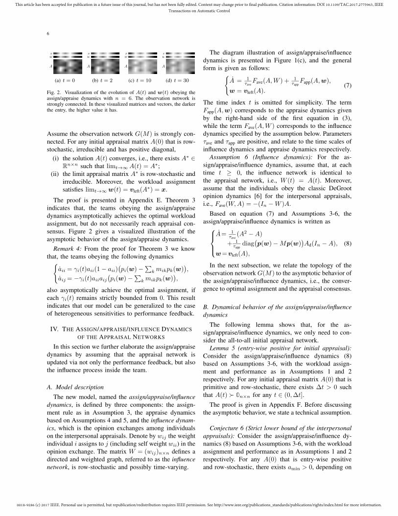
Fig. 2. Visualization of the evolution of A(t) and w(t) obeying theassign/appraise dynamics with n = 6. The observation network isstrongly connected. In these visualized matrices and vectors, the darkerthe entry, the higher value it has.

Assume the observation network G(M) is strongly con-nected. For any initial appraisal matrix A(0) that is row-stochastic, irreducible and has positive diagonal,

(i) the solution A(t) converges, i.e., there exists A∗ ∈Rn×n such that limt→∞A(t) = A∗;

(ii) the limit appraisal matrix A∗ is row-stochastic andirreducible. Moreover, the workload assignmentsatisfies limt→∞w(t) = vleft(A

∗) = x.

The proof is presented in Appendix E. Theorem 3indicates that, the teams obeying the assign/appraisedynamics asymptotically achieves the optimal workloadassignment, but do not necessarily reach appraisal con-sensus. Figure 2 gives a visualized illustration of theasymptotic behavior of the assign/appraise dynamics.

Remark 4: From the proof for Theorem 3 we knowthat, the teams obeying the following dynamics

aii = γi(t)aii(1− aii)(pi(w)−

∑kmikpk(w)

),

aij = −γi(t)aiiaij(pi(w)−

∑kmikpk(w)

),

also asymptotically achieve the optimal assignment, ifeach γi(t) remains strictly bounded from 0. This resultindicates that our model can be generalized to the caseof heterogeneous sensitivities to performance feedback.

IV. THE ASSIGN/APPRAISE/INFLUENCE DYNAMICSOF THE APPRAISAL NETWORKS

In this section we further elaborate the assign/appraisedynamics by assuming that the appraisal network isupdated via not only the performance feedback, but alsothe influence process inside the team.

A. Model description

The new model, named the assign/appraise/influencedynamics, is defined by three components: the assign-ment rule as in Assumption 3, the appraise dynamicsbased on Assumptions 4 and 5, and the influence dynam-ics, which is the opinion exchanges among individualson the interpersonal appraisals. Denote by wij the weightindividual i assigns to j (including self weight wii) in theopinion exchange. The matrix W = (wij)n×n defines adirected and weighted graph, referred to as the influencenetwork, is row-stochastic and possibly time-varying.

The diagram illustration of assign/appraise/influencedynamics is presented in Figure 1(c), and the generalform is given as follows:

A = 1τaveFave(A,W ) + 1

τappFapp(A,w),

w = vleft(A).(7)

The time index t is omitted for simplicity. The termFapp(A,w) corresponds to the appraise dynamics givenby the right-hand side of the first equation in (3),while the term Fave(A,W ) corresponds to the influencedynamics specified by the assumption below. Parametersτave and τapp are positive, and relate to the time scales ofinfluence dynamics and appraise dynamics respectively.

Assumption 6 (Influence dynamics): For the as-sign/appraise/influence dynamics, assume that, at eachtime t ≥ 0, the influence network is identical tothe appraisal network, i.e., W (t) = A(t). Moreover,assume that the individuals obey the classic DeGrootopinion dynamics [6] for the interpersonal appraisals,i.e., Fave(W,A) = −(In −W )A.

Based on equation (7) and Assumptions 3-6, theassign/appraise/influence dynamics is written as

A= 1τave

(A2 −A)

+ 1τapp

diag(p(w)−Mp(w)

)Ad(In −A),

w=vleft(A),

(8)

In the next subsection, we relate the topology of theobservation network G(M) to the asymptotic behavior ofthe assign/appraise/influence dynamics, i.e., the conver-gence to optimal assignment and the appraisal consensus.

B. Dynamical behavior of the assign/appraise/influencedynamics

The following lemma shows that, for the as-sign/appraise/influence dynamics, we only need to con-sider the all-to-all initial appraisal network.

Lemma 5 (entry-wise positive for initial appraisal):Consider the assign/appraise/influence dynamics (8)based on Assumptions 3-6, with the workload assign-ment and performance as in Assumptions 1 and 2respectively. For any initial appraisal matrix A(0) that isprimitive and row-stochastic, there exists ∆t > 0 suchthat A(t) 0n×n for any t ∈ (0,∆t].

The proof is given in Appendix F. Before discussingthe asymptotic behavior, we state a technical assumption.

Conjecture 6 (Strict lower bound of the interpersonalappraisals): Consider the assign/appraise/influence dy-namics (8) based on Assumptions 3-6, with the workloadassignment and performance as in Assumptions 1 and 2respectively. For any A(0) that is entry-wise positiveand row-stochastic, there exists amin > 0, depending on



7

A(0), such that A(t) amin1n1>n for any time t ≥ 0, aslong as A(τ) and w(τ) are well-defined for all τ ∈ [0, t].

Monte Carlo validation and a sufficient condition forConjecture 6 are presented in Appendix G. Now we statethe main results of this section.

Theorem 7 (Assign/appraise/influence dynamical be-havior): Consider the assign/appraise/influence dynam-ics (8) based on Assumptions 3-6, with the task assign-ment and performance as in Assumptions 1 and Assump-tion 2 respectively. Suppose that Conjecture 6 holds.Assume that the observation network G(M) contains aglobally reachable node. For any initial appraisal matrixA(0) that is entry-wise positive and row-stochastic, andany time scales τave > 0 and τapp > 0 in equation (8),

(i) the solution A(t) exists and w(t) = vleft(A(t)

)is well-defined for all t ∈ [0,+∞). Moreover,A(t) 0n×n and A(t)1n = 1n for any t ≥ 0;

(ii) the assignment w(t) obeys the generalized repli-cator dynamics (6), and ξ01n w(t)

(1− (n−

1)ξ0)1n, where

ξ0 =

(1 + (n− 1)

maxk xkminl xl

γ0

)−1, and

γ0 =maxk xk/wk(0)

minl xl/wl(0);

(iii) as t→ +∞, A(t) converges to 1nx> and therebyw(t) converges to x.

The proof is given in Appendix H. As Theorem 7indicates, the team obeying the assign/appraise/influencedynamics achieves collective learning. A visualized illus-tration of the dynamics is given by Figure 3.

Theorem 7 indicates that the asymptotic behaviorof the assign/appraise/influence dynamics is indepen-dent of the time scales τave and τapp. The followingargument adds some intuition to this observation. Theassign/appraise/influence dynamics can be regarded acombination of the assign/appraise dynamics (3) and theinfluence dynamics A = A2. As shown in Section III,for an appraisal matrix A(t) obeying the assign/appraisedynamics (3), the left dominant eigenvector vleft(A(t))converges to the optimal assignment x. Moreover, alongthe dynamics A = A2, the eigenvector vleft(A(t))remains unchanged. Theorem 7 states that the intro-duction of the influence dynamics does not affect theconvergence of the left dominant eigenvector of A(t) tox.

V. MODEL VARIATIONS: CAUSES OFFAILURE TO LEARN

The assign/appraise/influence dynamics (8) consists ofthree phases: the assignment rule, the appraise dynamics,and the influence dynamics. In this section, we proposeone variation in each of the three phases, based on some

xw

A

(a) t = 0

xw

A

(b) t = 2

xw

A

(c) t = 10

xw

A

(d) t = 30

Fig. 3. Visualization of the evolution of A(t) and w(t) obeying theassign/appraise/influence dynamics with n = 6. The observation net-work contains a globally reachable node. In these visualized matricesand vectors, the darker the entry, the higher value it has.

xw

A

(a) no influencedynamics, t = 0

xw

A

(b) no influencedynamics, t = 2

xw

A

(c) no influencedynamics, t =30

xw

A

(d) no influencedynamics, t =50

xw

A

(e) with influ-ence dynamics,t = 0

xw

A

(f) withinfluencedynamics, t = 2

xw

A

(g) with influ-ence dynamics,t = 30

xw

A

(h) with influ-ence dynamics,t = 50

Fig. 4. Examples of the assign/appraise (first row) and the as-sign/appraise/influence (second row) dynamics in which the assignmentis based on the individuals’ in-degree centrality. The assign/appraisedynamics does not achieve the collective learning, while the as-sign/appraise/influence dynamics does.

socio-psychological mechanisms that may cause a failurein team learning. We investigate the behavior of eachmodel variation by numerical simulation.

a) Variation in the assignment rule: workload as-signment based on degree centrality: In Assumption 3,the workload assignment is based on the individuals’eigenvector centrality in the appraisal network. If weassume instead that the assignment is based on the indi-viduals’ normalized in-degree centrality in the appraisalnetwork, i.e., w(t) = A>(t)1n/1>nA(t)1n, then thenumerical simulation, see Figure 4, shows the followingresults: the team obeying the assign/appraise dynamicsdoes not necessarily achieve collective learning, whilethe team obeying the assign/appraise/influence dynamicsstill achieves collective learning.

b) Variation in the appraise dynamics: partial ob-servation of performance feedback: According to As-sumption 4, the observation network G(M) determinesthe feedback signals received by each individual. If theobservation network does not have the desired connec-tivity property, the individuals do not have sufficientinformation to achieve collective learning. Simulationresults in Figure 5 shows that, if G(M) is not stronglyconnected for the assign/appraise dynamics, or if G(M)does not contain a globally reachable node for the



8

xw

A

(a) no influencedynamics, t = 0

xw

A

(b) no influencedynamics, t = 1

xw

A

(c) no influencedynamics, t = 5

xw

A

(d) no influencedynamics, t =10

xw

A

(e) with influ-ence dynamics,t = 0

xw

A

(f) withinfluencedynamics, t = 5

xw

A

(g) with influ-ence dynamics,t = 50

xw

A

(h) with influ-ence dynamics,t = 60

Fig. 5. Examples of failure to learn with partial observation fora six-individual team. The figures in the first row correspond tothe assign/appraise dynamics, in which the observation network isnot strongly connected but contains a globally reachable node. Thefigures in the second row correspond to the assign/appraise/influencedynamics, in which the observation network does not contain a globallyreachable node. In both cases, A(t) converges but lim

t→+∞w(t) 6= x.

xw

A

(a) t = 0

xw

A

(b) t = 1

xw

A

(c) t = 5

xw

A

(d) t = 10

Fig. 6. Example of the evolution of A(t) and w(t) in the prejudicemodel with n = 6. The darker the entry, the higher value it has. Thesimulation result shows that A(t) converges but w(t) = vleft

(A(t)

)does not necessarily converges to x.

assign/appraise/influence dynamics, the team does notnecessarily achieve collective learning.

c) Variation in the influence dynamics: prejudicemodel: In Assumption 6, we assume that the individualsobey the DeGroot opinion dynamics. If we instead adoptthe Friedkin-Johnsen opinion dynamics, given by

Fave(A,W ) = −Λ(In −W )A+ (In − Λ)(A(0)−A),

where Λ = diag(λ1, . . . , λn) and each λi characterizesindividual i’s attachment to her initial appraisals. Numer-ical simulation, see Figure 6, shows that the team doesnot necessarily achieve collective learning. The Friedkin-Johnsen model captures the social-psychological mech-anism in which individuals show an attachment to theirinitial opinions, which causes the failure to learn.

VI. FURTHER DISCUSSION AND CONCLUSION

A. Connections with TMS theory

TMS structure: As discussed in the introduction, oneimportant aspect of TMS is the members’ shared under-standing about who possess what expertise. For the caseof one-dimension skill, TMS structure is approximately

0 5 10 150

0.25

0.5

0.75

1

assign/appraise/influenceassign/appraiserandom assignment

t

eH1(w)

(a) e−H1(w,x)

0 5 10 150

20

40

60

80

assign/appraise/influenceassign/appraiserandom assignment

t

Nnon-transitive triads

(b) Number of non-transitive triads

Fig. 7. Evolution of the measure of mismatch between assignmentand individual skill levels, and the number of non-transitive triadsin the comparative appraisal graph. The solid curves represent theteam obeying the assign/appraise/influence dynamics. The dash curvesrepresent the team obeying the assign/appraise dynamics. The dottedcurves represent the team that randomly assign sub-task workloads.

characterized by the appraisal matrix and thus the devel-opment of TMS corresponds to the collective learningon individuals’ true skill levels. Simulation results inFigure 7 compare the evolution of some features amongthe teams obeying the assign/appraise/influence model,the assign/appraise model, and the team that randomlyassigns the sub-tasks, respectively. Figure 7(a) showsthat, for both the assign/appraise/influence dynamicsand the assign/appraise dynamics, the team performancemeasureH1(w), defined by the mismatch between work-load assignment and individual skill levels, converges to0, which exhibits the advantage of a developing TMS.

Transitive triads: As Palazzolo [24] points out, transi-tive triads are indicative of a well-organized TMS. Theunderlying logic is that inconsistency of interpersonalappraisals lowers the efficiency of locating the expertiseand allocating the incoming information. In order toreveal the evolution of triad transitivity in our models,we define an unweighted and directed graph, referredto as the comparative appraisal graph G(A) = (V,E),with V = 1, . . . , n, as follows: for any i, j ∈ V ,(i, j) ∈ E if aij ≥ aii, i.e., if individual i thinks j hasno lower skill level than i herself. We adopt the standardnotion of triad transitivity and use the number of non-transitive triads as the indicator of inconsistency in ateam. Figure 7(b) shows that, the non-transitive triadsvanish along the assign/appraise/influence dynamics, butpersist along the assign/appraise dynamics or the randomassignments.

B. Observation network structure and learning speed

Simulation results illustrate how the structure of theobservation network affects the convergence speeds ofour models, characterized by the convergence time Tc =min

t ≥ 0

∣∣ e−H1(w(t)) ≥ 0.99

. Tc is a function ofthe skill level x, the initial condition A(0), and theobservation network. We run 100 independent realiza-tions of the assign/appraise dynamics for a team with



9

0.2 0.4 0.6 0.8 10

0.25

0.5

0.75

1

plink

scaled Tc

(a) assign/appraise0.2 0.4 0.6 0.8 10

0.25

0.5

0.75

1

scaled Tc

plink

(b) assign/appraise/influence

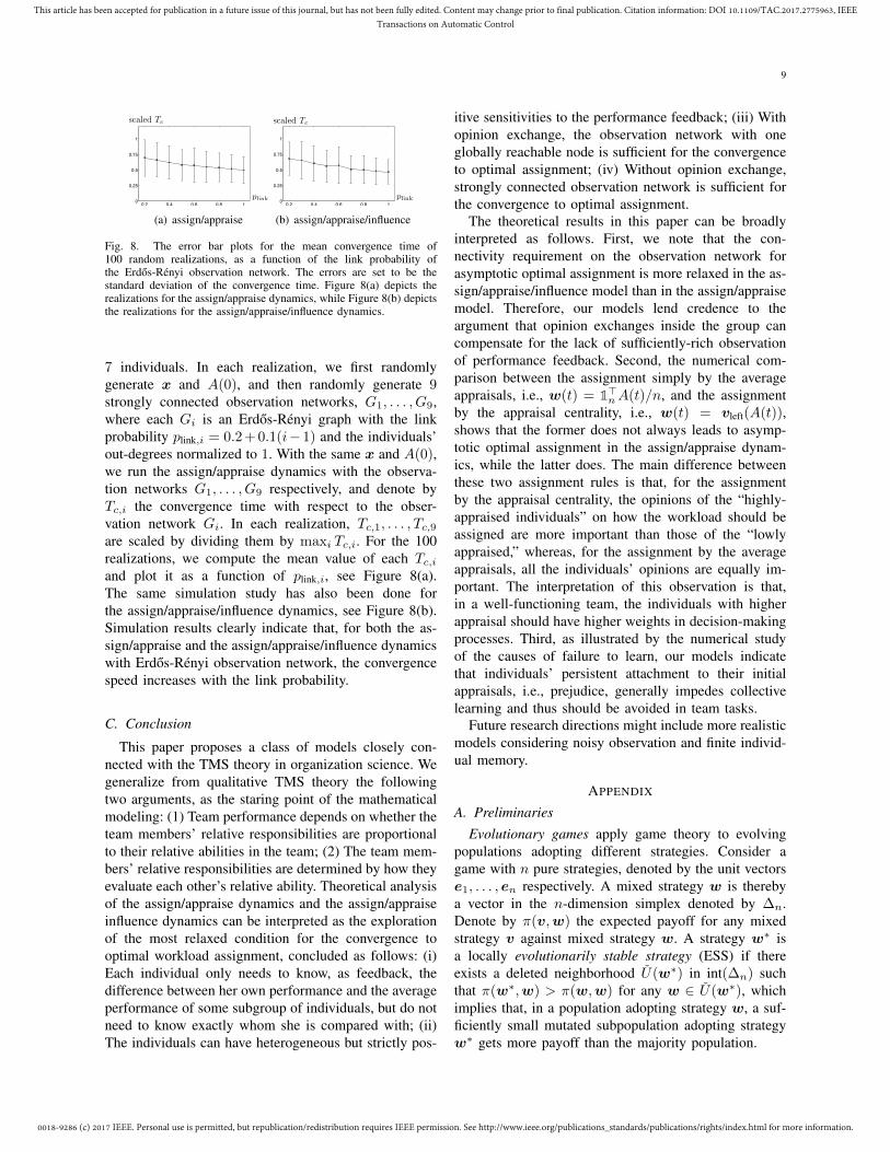
Fig. 8. The error bar plots for the mean convergence time of100 random realizations, as a function of the link probability ofthe Erdos-Renyi observation network. The errors are set to be thestandard deviation of the convergence time. Figure 8(a) depicts therealizations for the assign/appraise dynamics, while Figure 8(b) depictsthe realizations for the assign/appraise/influence dynamics.

7 individuals. In each realization, we first randomlygenerate x and A(0), and then randomly generate 9strongly connected observation networks, G1, . . . , G9,where each Gi is an Erdos-Renyi graph with the linkprobability plink,i = 0.2 + 0.1(i− 1) and the individuals’out-degrees normalized to 1. With the same x and A(0),we run the assign/appraise dynamics with the observa-tion networks G1, . . . , G9 respectively, and denote byTc,i the convergence time with respect to the obser-vation network Gi. In each realization, Tc,1, . . . , Tc,9are scaled by dividing them by maxi Tc,i. For the 100realizations, we compute the mean value of each Tc,iand plot it as a function of plink,i, see Figure 8(a).The same simulation study has also been done forthe assign/appraise/influence dynamics, see Figure 8(b).Simulation results clearly indicate that, for both the as-sign/appraise and the assign/appraise/influence dynamicswith Erdos-Renyi observation network, the convergencespeed increases with the link probability.

C. Conclusion

This paper proposes a class of models closely con-nected with the TMS theory in organization science. Wegeneralize from qualitative TMS theory the followingtwo arguments, as the staring point of the mathematicalmodeling: (1) Team performance depends on whether theteam members’ relative responsibilities are proportionalto their relative abilities in the team; (2) The team mem-bers’ relative responsibilities are determined by how theyevaluate each other’s relative ability. Theoretical analysisof the assign/appraise dynamics and the assign/appraiseinfluence dynamics can be interpreted as the explorationof the most relaxed condition for the convergence tooptimal workload assignment, concluded as follows: (i)Each individual only needs to know, as feedback, thedifference between her own performance and the averageperformance of some subgroup of individuals, but do notneed to know exactly whom she is compared with; (ii)The individuals can have heterogeneous but strictly pos-

itive sensitivities to the performance feedback; (iii) Withopinion exchange, the observation network with oneglobally reachable node is sufficient for the convergenceto optimal assignment; (iv) Without opinion exchange,strongly connected observation network is sufficient forthe convergence to optimal assignment.

The theoretical results in this paper can be broadlyinterpreted as follows. First, we note that the con-nectivity requirement on the observation network forasymptotic optimal assignment is more relaxed in the as-sign/appraise/influence model than in the assign/appraisemodel. Therefore, our models lend credence to theargument that opinion exchanges inside the group cancompensate for the lack of sufficiently-rich observationof performance feedback. Second, the numerical com-parison between the assignment simply by the averageappraisals, i.e., w(t) = 1>nA(t)/n, and the assignmentby the appraisal centrality, i.e., w(t) = vleft(A(t)),shows that the former does not always leads to asymp-totic optimal assignment in the assign/appraise dynam-ics, while the latter does. The main difference betweenthese two assignment rules is that, for the assignmentby the appraisal centrality, the opinions of the “highly-appraised individuals” on how the workload should beassigned are more important than those of the “lowlyappraised,” whereas, for the assignment by the averageappraisals, all the individuals’ opinions are equally im-portant. The interpretation of this observation is that,in a well-functioning team, the individuals with higherappraisal should have higher weights in decision-makingprocesses. Third, as illustrated by the numerical studyof the causes of failure to learn, our models indicatethat individuals’ persistent attachment to their initialappraisals, i.e., prejudice, generally impedes collectivelearning and thus should be avoided in team tasks.

Future research directions might include more realisticmodels considering noisy observation and finite individ-ual memory.

APPENDIX

A. PreliminariesEvolutionary games apply game theory to evolving

populations adopting different strategies. Consider agame with n pure strategies, denoted by the unit vectorse1, . . . , en respectively. A mixed strategy w is therebya vector in the n-dimension simplex denoted by ∆n.Denote by π(v,w) the expected payoff for any mixedstrategy v against mixed strategy w. A strategy w∗ isa locally evolutionarily stable strategy (ESS) if thereexists a deleted neighborhood U(w∗) in int(∆n) suchthat π(w∗,w) > π(w,w) for any w ∈ U(w∗), whichimplies that, in a population adopting strategy w, a suf-ficiently small mutated subpopulation adopting strategyw∗ gets more payoff than the majority population.



10

Replicator dynamics models the evolution of sub-populations adopting different strategies. The total pop-ulation is divided into n sub-populations. Individuals ineach sub-population i adopt the pure strategy ei. Denoteby wi(t) the fraction of sub-population i in the totalpopulation at time t. The fitness of sub-population i,denoted by πi

(w(t)

), depends on the sub-population

distribution w(t) =(w1(t), . . . , wn(t)

)>and is defined

as the expected payoff π(ei,w(t)

). The growth rate of

sub-population i is equal to the deviation of its fitnessfrom the population average. The replicator dynamics isgiven by:

wi = wi

(πi(w)−

n∑k=1

wkπk(w)). (9)

There is a simple connection between the locally ESSand the replicator dynamics [5]: Generally, a locally ESSin int(∆n) is a locally asymptotic equilibrium of thereplicator dynamics; Specifically, if there exists a matrixA such that π(v,w) = v>Aw for any v,w ∈ ∆n, thena locally ESS in int(∆n) is a globally asymptotic stableequilibrium of the replicator dynamics. In addition, thereplicator dynamics is also a mean-field approximationof some stochastic population process, which is out ofthe scope of this paper.

B. Proof for Theorem 1

The vector form of equation (1) is written as

w = diag(w)(p(w)−w>p(w)1n

). (10)

Left multiply both sides by 1>n . We get d(1>nw)/dt =0. Moreover, since wi = 0 whenever wi = 0, the n-dimension simplex ∆n is an positively invariant set.

Since the function f is continuously differentiable,the right-hand side of equation (10) is continuouslydifferentiable and locally Lipschitz in int(∆n). Define

V (w) = −n∑i=1

xi logwixi.

Due to the strict concavity of log function and 1>nw = 1,we have that V (w) ≥ 0 for any w ∈ ∆n and V (w) = 0if and only if w = x. Moreover, since V (w) iscontinuously differentiable in w, the level set w ∈int(∆n) |V (w) = ξ is a compact subset of int(∆n).Since the function f is monotonically increasing, alongthe trajectory,

dV (w)

dt= −

∑i∈θ1(w)

(xi − wi)f(xi/wi)

−∑

i∈θ2(w)

(xi − wi)f(xi/wi) < 0,

where θ1(w) = i |xi ≥ wi and θ2(w) = i |xi <wi. This concludes the proof for the invariant set andthe asymptotic stability of w∗ = x, and one can infer,from the inequality above, that w∗ = x is the ESS forthe evolutionary game with the payoff function πi(w) =f(xi/wi). Moreover, since V (w)→ +∞ as w tends tothe boundary of ∆n, the region of attraction is int(∆n).

C. Justifications of Assumption 3

We provide some justification of Assumption 3 onthe workload assignment rule w = vleft(A). Firstly, theentries of vleft(A) correspond to the individuals’ eigen-vector centrality in the appraisal network and thus reflecthow much each individual is appraised by the team. Sec-ondly, each row i of A(t) can be considered as individuali’s opinion on how to divide the workload for the taskat time t. Suppose the group of individuals exchangetheir opinions over the influence network defined byW = A(t) and eventually reach consensus on the work-load assignment. We have that the consensus workloadassigned to any individual j, denoted by wj(t), satisfieswj(t) = limk→∞W kAj(t) = 1nvleft(A(t))>Aj(t),whereAj(t) denotes the j-th column of A(t). Therefore,w>(t) = vleft(A(t))>A(t), which leads to w(t) =vleft(A(t)). Thirdly, our eigenvector assignment rule isconsistent with the following natural property: in a teamwithout performance feedback, , due to the lack ofinformation inflow, the team’s task assignment does notchange. These arguments justify Assumption 3; recallalso Section V a) with a numerical evaluation of adifferent assignment rule.

D. Proof for Theorem 2

Before the proof, we state a useful lemma summarizedfrom Page 62-67 of [31].

Lemma 8 (Continuity of eigenvalue and eigenvector):Suppose A,B ∈ Rn×n satisfy |aij | < 1 and |bij | < 1for any i, j ∈ 1, . . . , n. For sufficiently small ε > 0,

(i) the eigenvalues λ and λ′

of A and (A + εB),respectively, can be put in one-to-one correspon-dence so that |λ′ − λ| < 2(n+ 1)2(n2ε)

1n ;

(ii) if λ is a simple eigenvalue of A, then the cor-responding eigenvalue λ(ε) of A + εB satisfies|λ(ε)− λ| = O(ε);

(iii) if v is an eigenvector of A associated with a simpleeigenvalue λ, then the eigenvector v(ε) of A+ εBassociated with the corresponding eigenvalue λ(ε)satisfies |vi(ε)−vi| = O(ε) for any i ∈ 1, . . . , n.

Proof of Theorem 2: In this proof, we extend thedefinition of vleft(A) to the normalized entry-wise posi-tive left eigenvector, associated with the eigenvalue of Awith the largest magnitude, if such an eigenvector exists



11

and is unique. According to Perron-Frobenius theoremand Lemma 8, vector vleft(A), as long as well-defined,depends continuously on the entries of A. Therefore,for system (3), there exists a sufficiently small τ > 0such that A(t) and w(t) are well-defined and contin-uously differentiable at any t ∈ [0, τ ], and, moreover,pi(w(t)

)−∑kmikpk

(w(t)

)remains finite. Therefore,

for any t ∈ [0, τ ] and i, j ∈ 1, . . . , n, aij(t) > 0 ifaij(0) > 0; aij(t) = 0 if aij(0) = 0, and thus A(t) isrow-stochastic and primitive for any t ∈ [0, τ ].

For any i ∈ 1, . . . , n, there exists k 6= i such thataik(0) > 0. According to equation (2),

daij(t)

daik(t)=aij(t)

aik(t), ∀t ∈ [0, τ ], ∀j ∈ 1, . . . , n\i, k,

which leads to aij(t)/aik(t) = aij(0)/aik(0). Let C bean n×n matrix with the entries cij defined as: (i) cii = 0for any i ∈ 1, . . . , n; (ii) cij = aij(0)

/(1−aii(0)

)for

any j 6= i. One can check that C is row-stochastic andA(t) is given by equation (4), for any t ∈ [0, τ ], wherea(t) =

(a1(t), . . . , an(t)

)>with ai(t) = aii(t). Since

the digraph, with C as the adjacency matrix, has thesame topology with the digraph associated with A(0),matrix C is irreducible and c = vleft(C) is well-defined.

Since the matrix A(t) has the structure given by (4),according to Lemma 2.2 in [12], for any t ∈ [0, τ ],

wi(t) =ci

1− ai(t)

/∑k

ck1− ak(t)

.

Therefore, for any t ∈ [0, τ ],

pi(w(t)

)= f

(xici

(1− ai(t)

)∑k

wk(t)ck

1− ak(t)

).

According to equation (2), aj(t) ≤ 0 for any j ∈argmink

xkck

(1 − ak(t)

). Therefore, argmink

xkck

(1 −

ak(t))

is increasing, and similarly, argmaxkxkck

(1 −

ak(t))

is decreasing with t, which implies that, the set

ΩA(A(0)

)=A ∈ Rn×n

∣∣∣A = diag(a) + (I − diag(a))C,

0 ≤ ai ≤ 1− cixi

mink

xkck

(1− akk(0)

),∀i

is a compact positive invariant set for system (3), as longas A(0) is row-stochastic, irreducible and has strictlypositive diagonal. Moreover, one can check that, for anyA ∈ ΩA

(A(0)

),w = vleft(A) is well-defined and strictly

lower (upper resp.) bounded from 0 (1 resp.). Therefore,the solution A(t) is extensible to all t ∈ [0,+∞)and equations (4) and (5) hold for any t ∈ [0,+∞).Moreover, since pi

(w(t)

)−∑kmikpk

(w(t)

)remains

bounded, we have aij > 0 if aij(0) > 0 and aij(t) = 0if aij(0) = 0. This concludes the proof for (i) - (iv).

For statement (v), differentiate both sides of the equa-tion w>(t)A(t) = w>(t) and substitute equation (3)into the differentiated equation. We obtain

(w>diag(p(w)−Mp(w))Ad −dw>

dt)(In −A) = 0>n ,

where time index t is omitted for simplicity. Equation (6)in statement (v) is obtained due to w>(t)1n = 1.

E. Proof for Theorem 3

We prove the theorem by analyzing the generalizedreplicator dynamics (6) for w(t), and the reduced as-sign/appraise dynamics (5) for a(t), given any constant,normalized and entry-wise positive vector c. Accordingto equation (5), the assignment w = vleft(A) can beconsidered as a function of the self appraisal vectora, that is, w(t) = w

(a(t)

)for any t ≥ 0. In this

proof, let φ(a) = p(w(a)

)−Mp

(w(a)

)and denote

by D : Rn × Rn → R≥0 the distance induced by the2-norm in Rn. For any x ∈ Rn and subset S of Rn,defined D(x, S) = infy∈S D(x,y).

First of all, for any given a(0) ∈ (0, 1)n, we knowthat the set Ω, as defined in Theorem 2(iv), is a compactpositively invariant set for dynamics (5), and w(t) iswell-defined and entry-wise strictly lower (upper resp.)bounded from 0n (1n resp.), for all t ∈ [0,+∞).

Secondly, for any a ∈ Ω, define a scalar functionV : Rn → R as

V (a) = logmaxk xk/wk(a)

mink xk/wk(a),

and the following index sets

θ(a) =i∣∣∣ ∃ti > 0 s.t.

xi

wi(a(t)

) = maxk

xk

wk(a(t)

)for any t ∈ [0, ti], with a(0) = a

, and

θ(a) =j∣∣∣ ∃tj > 0 s.t.

xj

wj(a(t)

) = mink

xk

wk(a(t)

)for any t ∈ [0, tj ], with a(0) = a

.

Then the right time derivative of V(a(t)

), along the

solution a(t), is given by

d+V(a(t)

)dt

= aj(t)φj(a(t)

)− ai(t)φi

(a(t)

),

for any i ∈ θ(a(t)

)and j ∈ θ

(a(t)

). Define

E =a ∈ Ω

∣∣ ajφj(a)− aiφi(a) = 0

for any i ∈ θ(a), j ∈ θ(a),

E1 =a ∈ E

∣∣φ(a) = 0n,

E2 =a ∈ E

∣∣φ(a) 6= 0n.



12

One can check that E and E1 are compact subsetsof Ω, E = E1 ∪ E2, and E1 ∩ E2 is empty. Denoteby E the largest invariant subset of E. Applying theLaSalle Invariance Principle, see Theorem 3 in [13],we have D

(a(t), E

)→ 0 as t → +∞. Note that,

limt→+∞

D(a(t), E

)= 0 does not necessarily leads to

limt→+∞

w(t) = x. We need to further refine the result.

For set E1, it is straightforward to see that E1 ⊂ Eand w(a) = x for any a ∈ E1. Now we prove bycontradiction that, if E2 ∩ E is not empty, then, forany a ∈ E2 ∩ E, there exists i ∈ θ(a) such thatai = 0. Suppose ai > 0 for any i ∈ θ(a). Since theobservation network G(M) is strongly connected, thereexists a directed path i, k1, . . . , kq, j on G(M), wherei ∈ θ(a) and j ∈ θ(a). We have k1 ∈ θ(a), otherwise,starting with a(0) = a, there exists sufficiently small∆t > 0 such that φi

(a(t)

)> 0 and ai(t) > 0, which

contradicts the fact that a is in the largest invariant setof E. Repeating this argument, we have j ∈ θ(a), whichcontradicts φ(a) 6= 0n. Similarly, we have that, for anya ∈ E2 ∩ E, there exists j ∈ θ(a) with aj = 0.

If the fixed vectors c and x satisfy c = x, then therecan not exist a ∈ E2∩E satisfying all the following threeproperties: i) there exists i ∈ θ(a) such that ai = 0; ii)there exists j ∈ θ(a) such that aj = 0; iii) φ(a) 6= 0n.In this case, E2 ∩ E is an empty set, which implies thata(t)→ E = E1 and thus w(t)→ x as t→ +∞.

Before discussing the case when c 6= x, we presentsome properties of the individual performance measure:

P1: For any k, l ∈ 1, . . . , n, xkck (1−ak) ≤ xlcl

(1−al)leads to pk(a) ≤ pl(a), and xk

ck(1 − ak) > xl

cl(1 − al)

leads to pk(a) > pl(a);P2: If there exists τ ≥ 0 such that i ∈ θ

(a(τ)

)and

ai(τ) = 0, then i ∈ θ(a(t)

)for all t ≥ τ ;

P3: p(a(t)) is finite and strictly bounded from0, satisfying f

(xici

(1 − ζi(a(0))))≤ pi(a(t)) ≤

f(xici

∑k

ckζk(a(0))

), with ζi(a) defined in Theorem 2(iv).

For the case when c 6= x, consider the partitionϕ1, . . . , ϕm of the index set 1, . . . , n, with m ≤ n,satisfying the following two properties:

(i) xk/ck = xl/cl for any k, l in the same subset ϕr;(ii) xk/ck > xl/cl for any k ∈ ϕr, l ∈ ϕs, with r < s.

For any a ∈ E2 ∩ E, since there exists j ∈ θ(a) withaj = 0, we have ϕm ⊂ θ(a). For any i ∈ ∪m−1r=1 ϕr, let

E2,i =a ∈ Ω

∣∣∣ ai = 0, aj = 0 for any j ∈ ϕm,

1− xici

ckxk≤ ak ≤ 1− min

l∈1,...,nxlcl

ckxk,

for any k ∈ ϕ1 ∪ · · · ∪ ϕm−1 \ i.

With properties P1 and P2 of p(a), for any a ∈ E2,i,we have i ∈ θ(a) and ai = 0. Moreover,

(i) E2,i ⊂ Rn is compact for any i ∈ ϕ1∪· · ·∪ϕm−1;(ii) ∪i∈ϕ1

E2,i, . . . ,∪i∈ϕm−1E2,i are disjoint and com-

pact subsets of Rn;(iii) E2 ∩ E ⊂

⋃i∈ϕ1∪···∪ϕm−1

E2,i.

For any a ∈ E2 ∩ E, since there exists i ∈ θ(a) andj ∈ θ(a) such that ai = aj = 0, on the observationnetwork G(M), there must exists a path i, k1, . . . , kqsatisfying: i) i ∈ θ(a) and ai = 0; ii) akq = 0 andxkq/ckq < xi/ci; iii) akl > 0 for any l ∈ 1, . . . , q−1.Consider the trajectory a(t) with a(0) = a, we have

˙akq−1≥ akq−1

(1− akq−1)

·(f(xkq−1

ckq−1

(1− akq−1)n∑l=1

cl1− al

)− f((mkq−1kq

xkqckq

+ (1−mkq−1kq )xici

) n∑l=1

cl1− al

)).

The inequality is due to properties P1-P3 of pi(a) fori ∈ θ(a) with ai = 0, and the concavity of the functionf . Moreover, since akq−1

is strictly bounded from 1 and∑l cl/(1 − al) is strictly lower bounded from 0, there

exists Tkq−1(M,a(0),a) > 0 such that

pkq−1

(a(t)

)<

2−mkq−1kq

2pi(a(t)

)+mkq−1kq

2pkq(a(t)

).

Applying the same argument to kq−2, . . . , k1, wehave that, there exists Tk1(M,a(0),a) > 0 andηik1...kq (M) ∈ (0, 1) such that, for the solution a(t)with a(0) = a,

pk1(a(t)

)<(1− ηik1...kq (M)

)pi(a(t)

)+ ηik1...kq (M)pkq

(a(t)

),

for all t ≥ Tk1(M,a(0),a). This inequality implies that,

φi(a(t)

)≥ mik1ηik1...kq (M)

(pi(a(t)

)− pkq

(a(t)

))≥ mik1ηik1...kq (M)f ′

(xici

)·n∑l=1

cl

1− ζl(a(0)

)(xici−xkqckq

)> 0.

Since the choices of i and the paths i, k1, . . . , kq arefinite, there exists a constant η > 0 such that, for anya ∈ E2 ∩ E, there exists T

(a(0),a

)> 0 such that,

for any t ≥ T(a(0),a

)> 0, the solution a(t), with

a(0) = a, satisfies i ∈ θ(a(t)

)and φi

(a(t)

)≥ η > 0.

For any i ∈ ϕ1 ∪ · · · ∪ ϕm−1, define

E2,i =a ∈ E2,i

∣∣ pi(a)−n∑k=1

mikpk(a) ≥ η.

We have: i) each E2,i is a compact subset of Rn; ii)∪i∈ϕ1

E2,i, . . . ,∪i∈ϕm−1E2,i are disjoint and compact



13

subsets of Rn. Let E2 = ∪m−1r=1

(∪r∈ϕr E2,i

). For

dynamics (5), due to the continuous dependency on theinitial condition, for any a ∈ (E2 ∩ E) \ (E2 ∩ E), thereexists δ > 0 such that, for any a(0) ∈ U(a, δ)∩(E2∩E),where U(a, δ) =

b ∈ Ω

∣∣D(b,a) ≤ δ

, a(t) ∈ E2∩ Efor sufficiently large t. Therefore, a can not be an ω-limit point of a(0). We thus obtain that, the ω-limit setof a(0) is in the set E1 ∪ (E2 ∩ E). Moreover, sinceE1,∪i∈ϕ1

E2,i, . . . ,∪i∈ϕm−1E2,i are disjoints compact

subsets of Rn, and the ω-limit set of a(0) is connectedand compact, a(t) can only converge to one of the setsE1,∪i∈ϕ1

E2,i, . . . ,∪i∈ϕm−1E2,i.

Now we prove limt→+∞D(a(t), E1) = 0 by contra-diction. Suppose ω

(a(0)

)∈ ∪i∈ϕr E2,i for some r ∈

1, . . . ,m− 1. Since each E2,i is a compact set, thereexists ε > 0 and η(ε) > 0 such that φi(a) ≥ η(ε) > 0for any a ∈ U(E2,i, ε). For this given ε > 0, sinceω(a(0)

)∈ ∪i∈ϕr E2,i leads to D

(a(t),∪i∈ϕr E2,i

)→ 0

as t→ +∞, we conclude that, there exists T > 0 suchthat, for any t ≥ T , a(t) ∈ ∪i∈ϕrU(E2,i, ε). DefineVr(a) = mini∈ϕr ai, for any a ∈ ∪i∈ϕrU(E2,i, ε).The function Vr(a) satisfies that, Vr(a) ≥ 0 for anya ∈ ∪i∈ϕrU(E2,i, ε) and Vr(a) = 0 if and only ifa ∈ ∪i∈ϕr E2,i. Therefore, D

(a(t),∪i∈ϕr E2,i

)→ 0

leads to Vr(a(t)

)→ 0 as t → +∞. Moreover, since

a ∈ U(E2,i, ε) for any i ∈ argmink∈ϕr ak, we have

d+Vr(a(t)

)dt

= mini∈argmin

k∈ϕrak(t)

ai(t) ≥ δai(t)(1− ai(t)

).

According to Theorem 2(i), for any given a(0) ∈(0, 1)n, a(t) ∈ (0, 1)n for all t ≥ 0. Therefore,d+Vr(a(t))/dt > 0 for all t ≥ T , which contra-dicts limt→+∞ Vr

(a(t)

)= 0. Therefore, we have

limt→+∞D(a(t), E1) = 0 and limt→+∞w(t) = x.Since A(t) → 0n×n as φ

(a(t)

)→ 0n, there exists

an entry-wise non-negative and irreducible matrix A∗,depending on A(0) and satisfying vleft(A

∗) = x, suchthat A(t)→ A∗ as t→ +∞. This concludes the proof.

F. Proof for Lemma 5Since A(0) is primitive and row-stochastic, following

the same argument in the proof for Theorem 2(i), wehave that, there exists ∆t > 0 such that, for any t ∈[0,∆t]: i) w(t) is well-defined and w(t) 0n; ii) A(t)is bounded, continuously differentiable to t, and satisfiesA(t)1n = 1n; iii) p

(w(t)

)− Mp

(w(t)

)is bounded.

Therefore, for any t ≥ 0, there exists µ, depending on tand A(0), such that A(t) 1

τaveA2(t)− ( 1

τave+ µ)A(t).

Consider the equation B(t) = 1τaveB2(t) − ( 1

τave+

µ)B(t), with B(0) = A(0). According to the compari-son theorem, A(t) B(t) for any t ≥ 0. Let bi(t) bethe i-th column of B(t) and let yk(t) = e(

1τave

+µ)tbk(t).We obtain yk(t) = 1

τaveB(t)yk(t).

Denote by Φ(t, 0) the state transition function for theequation yk(t) = 1

τaveB(t)yk(t), which is written as

Φ(t, 0) = In+∑∞k=1 Φk(t), where Φ1(t) =

∫ t0B(τ1)dτ1

and Φl(t) =∫ t0B(τ1)

∫ τ10. . . B(τl−1)

∫ τl−1

0B(τl)dτl

for l ≥ 2. By computing the MacLaurin expansion foreach Φk(t) and summing them together, we obtain that

Φ(t, 0) = In + h1(t)B(0) + h2(t)B2(0) + . . .

+ hn−1(t)Bn−1(0) +O(tn),

where hk(t) is a polynomial with the form hk(t) =ηk,kt

k + ηk,k+1tk+1 + . . . , and, moreover, ηk,k > 0

for any k ∈ N. Therefore, for t sufficiently small,we have hk(t) > 0 for any k ∈ 1, . . . , n − 1.Moreover, since Bk(0) 0n×n for any k ∈ N andB(0) + · · · + Bn−1(0) 0n×n, there exists ∆t ≤ ∆tsuch that Φ(t, 0) 0n×n for any t ∈ [0,∆t].

G. Discussion on Conjecture 6

The Monte Carlo method [28] is adopted to estimatethe probability that Conjecture 6 holds. For any ran-domly generated A(0) ∈ int(∆n), define the randomvariable Z : int(∆n)→ 0, 1 as

(i) Z(A(0)

)= 1 if there exists amin > 0 such that

A(t) amin1n1>n for all t ∈ [0, 1000];(ii) Z

(A(0)

)= 0 otherwise.

Let p = P[Z(A(0)

)= 1

]. For N independent random

samples Z1, . . . , ZN , in each of which A(0) is randomlygenerated in int(∆n), define pN =

∑Ni=1 Zi/N . For any

accuracy 1 − ε ∈ (0, 1) and confidence level 1 − ξ ∈(0, 1), |pN − p| < ε with probability greater than 1− ξif

N ≥ 1

2ε2log

2

ξ. (11)

For ε = ξ = 0.01, the Chernoff bound (11) is satisfiedby N = 27000. We run 27000 independent MATLABsimulations of the assign.appraise/influence dynamicswith n = 7 and find that pN = 1. Therefore, for anyA(0) ∈ int(∆n), with 99% confidence level, there isat least 0.99 probability that A(t) is entry-wise strictlylower bounded from 0n×n for all t ∈ [0, 10000].

Moreover, we present in the following lemma a suffi-cient condition for Conjecture 6 on the initial appraisalmatrix A(0) and the parameters τave, τapp.

Lemma 9 (Strictly positive lower bound of appraisals):Consider the assign/appraise/influence dynamics (8),based on Assumptions 3-6, with the assignment w(t)and performance p(w) as in Assumptions 1 and 2respectively. For any initial appraisal matrix A(0) thatis entry-wise positive and row-stochastic, as long as

τapp

τave≥ 1− ξ0

ξ0

(f

(xmax

ξ0

)− f

(xmin

1− (n− 1)ξ0

)),



14

where the constant ξ0 is defined as in Theorem 7 (ii),then there exists amin > 0 such that A(t) amin1n1>n .Proof: First of all, by definition we have ws(t) =∑k wk(t)aks(t). The right-hand side of this equation is a

convex combination of a1s(t), . . . , ans(t). Therefore,maxk aks(t) ≥ ws(t) ≥ ξ0 for all t ∈ [0,+∞).

At any time t ≥ 0, for any pair (i, j) such thataij(t) = mink,l akl(t), the dynamics for aij(t) is

aij(t) =1

τave

(∑k

aik(t)akj(t)− aij(t)

)

− 1

τappaii(t)aij(t)

(pi(w(t)

)−

n∑k=1

mikpk(w(t)

)).

For simplicity, in this proof, denote φi = pi(w(t)

)−∑n

k=1mikpk(w(t)

). Suppose amj(t) = maxk akj(t).

We have

aij(t) ≥1

τaveaij(t)amj(t)−

1

τavea2ij(t)

− 1

τappaii(t)aij(t)φi.

Therefore,aijaij≥ 1

τaveξ0 −

1

τapp(1− ξ0)

(f(xmax

ξ0

)− f

( xmin

1− (n− 1)ξ0

)).

The condition on 1τave/ 1τapp

in Lemma 9 guarantees thataij(t)

/aij(t) is positive if aij(t) = mink,l akl(t). This

concludes the proof.

H. Proof for Theorem 7Statement (i) is proved following the same argument

in the proof for Theorem 2 (i). For any given A(0)that is row-stochastic and entry-wise positive, the closedand bounded invariant set Ω for A(t) is given byΩ =

A ∈ Rn×n

∣∣A amin1n1>n , A1n = 1n

, whereamin > 0 is given by Conjecture 6.

Since w>(t)(A2(t) − A(t)

)= 0>n for all t ≥ 0,

we conclude that, w(t) in the assign/appraise/influencedynamics also obeys the generalized replicator dynam-ics (6). Consider w(t) as a function of A(t). Defineφ(A) = p

(w(A)

)−Mp

(w(A)

)and

V (A) = logmaxk xk/wk(A)

mink xk/wk(A).

For any t ∈ [0,+∞), there exists i ∈argmaxk xk/wk

(A(t)

)and j ∈ argmink xk/wk

(A(t)

)such that V

(A(t)

)= log

(xiwj

(A(t)

)/xjwi

(A(t)

)),

and d+V (A)dt = ajjφj(A) − aiiφi(A) ≤ 0. Therefore,

V(A(t)

)is non-increasing with t, which in turn implies

xixj

wj(t)

wi(t)≤ maxk xk/wk(0)

mink xk/wk(0)= γ0,

for any i, j ∈ 1, . . . , n. This inequality, combined withthe fact that

∑k wk(t) = 1 for any t ≥ 0, leads to the

inequalities in statement (ii).Similar to the proof for Theorem 3, define

θ(A) =i∣∣∣∃ ti > 0 s.t.

xi

wi(A(t)

) = maxk

xk

wk(A(t)

)for any t ∈ [0, ti] with A(0) = A

,

θ(A) =j∣∣∣∃ tj > 0 s.t.

xj

wj(A(t)

) = mink

xk

wk(A(t)

)for any t ∈ [0, tj ] with A(0) = A

,

and let E =A ∈ Ω

∣∣ d+V (A)/dt = 0

. For any A ∈E, since A amin1n1>n , we have φi(A) = φj(A) = 0for any i ∈ θ(A) and j ∈ θ(A). Suppose individual sis a globally reachable node in the observation network.There exists a directed path i, k1, . . . , kq, s. Without lossof generality, suppose q ≥ 1. For any A in the largestinvariant subset of E, we have k1 ∈ θ(A) and thereforeφk1(A) = 0. This iteration of argument leads to s ∈θ(A). Following the same line of argument, we haves ∈ θ(A). Therefore, for any given A(0) 0n×n thatis row-stochastic, the solution A(t) converges to E =A ∈ Ω |φ(A) = 0n = A ∈ Ω |vleft(A) = x.

Let A = maxj(

maxk akj − mink akj). One can

check that d+V (A)/dt along the dynamics (8) is acontinuous function of A for any A ∈ Ω. DefineEε/2 =

A ∈ E

∣∣ ‖A − 1nx>‖2 ≥ ε/2

. SinceE is compact, Eε/2 is also a compact set. For anyA ∈ Eε/2, since d+V (A)/dt is strictly negative anddepends continuously on A, there exists a neighborhoodU(A, rA) = A ∈ Ω | ‖A − A‖2 ≤ rA such thatd+V (A)/dt < 0 for any A ∈ U(A, rA). Due tothe compactness of Eε/2 and according to the Heine-Borel finite cover theorem, there exists K ∈ N andAk, rkk∈1,...,K, where Ak ∈ Eε/2 and rk > 0 forany k ∈ 1, . . . ,K, such that Eε/2 ⊂ ∪Kk=1U(Ak, rk).

Define the distance D : Rn × Rn → R≥0 as in theproof for Theorem 3. Let δ = minr1, . . . , rk, ε/2 and

B1 =A ∈ Ω

∣∣D(A, E) ≤ δ,D(A, Eε/2) > δ,

B2 =A ∈ Ω

∣∣D(A, E) ≤ δ,D(A, Eε/2) ≤ δ.

We have B1 ∩ B2 is empty. For any A ∈ B1,since D(A, E) ≤ δ, D(A, Eε/2) > δ, there ex-ists A ∈ Eε/2 such that D(A, A) ≤ δ. SinceD(A,1nx>) < ε/2, we have D(A,1nx>) ≤ D(A, A)+D(A,1nx>) < ε. Therefore, B1 ⊂ U(1nx>, ε). More-over, since B2 is compact, V (A) is lower bounded andd+V (A)/dt is strictly upper bounded from 0 in B2.Since limt→+∞D(A(t), E) = 0, there exists t0 > 0such that A(t) ∈ B1 ∪B2 for any t ≥ 0. Therefore, forany t ≥ t0, there exists t1 ≥ t such that A(t1) ∈ B1.



15

This argument is valid for any ε > 0, which implies that1nx> is an ω-limit point for any given A(0).

Since E is compact, D(A, E) is strictly positive. Sincelimt→+∞D

(A(t), E

)= 0, any A ∈ Ω\E can not be an

ω-limit point of A(0). For any A ∈ E \ 1nx>, sincethe solution passing through A asymptotically convergesto 1nx>, A ∈ E \ 1nx> can not be an ω-limit pointof A(0) either. Therefore, the ω-limit set of A(0) is1nx>. This concludes the proof.

REFERENCES

[1] E. G. Anderson Jr and K. Lewis. A dynamic model of individualand collective learning amid disruption. Organization Science,25(2):356–376, 2013. doi:10.1287/orsc.2013.0854.

[2] J. Barreiro-Gomez, N. Quijano, and C. Ocampo-Martinez. Con-strained distributed optimization: A population dynamics ap-proach. Automatica, 69:101–116, 2016. doi:10.1016/j.automatica.2016.02.004.

[3] S. Boyd, A. Ghosh, B. Prabhakar, and D. Shah. Random-ized gossip algorithms. IEEE Transactions on InformationTheory, 52(6):2508–2530, 2006. doi:10.1109/TIT.2006.874516.

[4] S. Y. Choi, H. Lee, and Y. Yoo. The impact of information tech-nology and transactive memory systems on knowledge sharing,application, and team performance: A field study. ManagementInformation System Quarterly, 34(4):855–870, 2010. URL:http://www.jstor.org/stable/25750708.

[5] R. Cressman and Y. Tao. The replicator equation and othergame dynamics. Proceedings of the National Academy ofSciences, 111:10810–10817, 2014. doi:10.1073/pnas.1400823111.

[6] M. H. DeGroot. Reaching a consensus. Journal of theAmerican Statistical Association, 69(345):118–121, 1974. doi:10.1080/01621459.1974.10480137.

[7] L. Festinger. A theory of social comparison processes.Human Relations, 7(2):117–140, 1954. doi:10.1177/001872675400700202.

[8] N. E. Friedkin. A formal theory of reflected appraisals in theevolution of power. Administrative Science Quarterly, 56(4):501–529, 2011. doi:10.1177/0001839212441349.

[9] N. E. Friedkin and C. E. Johnsen. Attitude change, affect control,and expectation states in the formation of influence networks.Advances in Group Processes, 20:1–29, 2003. doi:10.1016/S0882-6145(03)20001-1.

[10] A. Jadbabaie, A. Sandroni, and A. Tahbaz-Salehi. Non-Bayesiansocial learning. Games and Economic Behavior, 76(1):210–225,2012. doi:10.1016/j.geb.2012.06.001.

[11] P. Jia, N. E. Friedkin, and F. Bullo. The coevolution of appraisaland influence networks leads to structural balance. IEEE Transac-tions on Network Science and Engineering, 3(4):286–298, 2016.doi:10.1109/TNSE.2016.2600058.

[12] P. Jia, A. MirTabatabaei, N. E. Friedkin, and F. Bullo. Opiniondynamics and the evolution of social power in influence net-works. SIAM Review, 57(3):367–397, 2015. doi:10.1137/130913250.

[13] J. P. LaSalle. Stability theory for ordinary differential equations.Journal of Differential Equations, 4:57–65, 1968. doi:10.1016/0022-0396(68)90048-X.

[14] J. Y. Lee, D. G. Bachrach, and K. Lewis. Social network ties,transactive memory, and performance in groups. OrganizationScience, 25(3):951–967, 2014. doi:10.1287/orsc.2013.0884.

[15] K. Lewis. Measuring transactive memory systems in the field:Scale development and validation. Journal of Applied Psychol-ogy, 88(4):587–604, 2003. doi:10.1037/0021-9010.88.4.587.

[16] K. Lewis. Knowledge and performance in knowledge-workerteams: A longitudinal study of transactive memory systems.Management Science, 50:1519–1533, 2004. doi:10.1287/mnsc.1040.0257.

[17] D. W. Liang, R. Moreland, and L. Argote. Group versusindividual training and group performance: The mediating role oftransactive memory. Personality and Social Psychology Bulletin,21:384–393, 1995. doi:10.1177/0146167295214009.

[18] J. Lorenz and D. A. Lorenz. On conditions for convergence toconsensus. IEEE Transactions on Automatic Control, 55:1651–1656, 2010. doi:10.1109/TAC.2010.2046086.

[19] D. Madeo and C. Mocenni. Game interactions and dynamics onnetworked populations. IEEE Transactions on Automatic Control,60:1801–1810, 2015. doi:10.1109/TAC.2014.2384755.

[20] J. G. March. Exploration and exploitation in organizationallearning. Organization Science, 2(1):71–87, 1991. doi:10.1287/orsc.2.1.71.

[21] J. R. Marden, H. P. Young, G. Arslan, and J. S. Shamma. Payoff-based dynamics for multiplayer weakly acyclic games. SIAMJournal on Control and Optimization, 48(1):373–396, 2009.doi:10.1137/070680199.

[22] W. Mei, N. E. Friedkin, K. Lewis, and F. Bullo. Dynamicmodels of appraisal networks explaining collective learning. InIEEE Conf. on Decision and Control, pages 3554–3559, LasVegas, NV, USA, December 2016. doi:10.1109/CDC.2016.7798803.

[23] A. Nedic and A. Ozdaglar. Distributed subgradient methodsfor multi-agent optimization. IEEE Transactions on AutomaticControl, 54(1):48–61, 2009. doi:10.1109/TAC.2008.2009515.

[24] E. T. Palazzolo. Organizing for information retrieval in transac-tive memory systems. Communication Research, 32(6):726–761,2005. doi:10.1177/0093650205281056.

[25] E. T. Palazzolo, D. A. Serb, Y. C. She, C. K. Su, and N. S. Con-tractor. Coevolution of communication and knowledge networksin transactive memory systems: Using computational models fortheoretical development. Communication Theory, 16:223–250,2006. doi:10.1111/j.1468-2885.2006.00269.x.

[26] Y. Ren, K. M. Carley, and L. Argote. The contingent effects oftransactive memory: When is it more beneficial to know whatothers know? Management Science, 52:671–682, 2006. doi:10.1287/mnsc.1050.0496.

[27] W. H. Sandholm. Population Games and Evolutionary Dynamics.MIT Press, 2010.

[28] R. Tempo, G. Calafiore, and F. Dabbene. Randomized Algorithmsfor Analysis and Control of Uncertain Systems. Springer, 2005.

[29] D. M. Wegner. Transactive memory: A contemporary analysisof the group mind. In B. Mullen and G. R. Goethals, editors,Theories of Group Behavior, pages 185–208. Springer, 1987.doi:10.1007/978-1-4612-4634-3_9.

[30] D. M. Wegner, R. Erber, and P. Raymond. Transactive memory inclose relationships. Journal of Personality and Social Psychology,61:923–929, 1991. doi:10.1037/0022-3514.61.6.923.

[31] J. H. Wilkinson. The Algebraic Eigenvalue Problem. OxfordUniversity Press, 1965.

[32] A. W. Woolley, C. F. Chabris, A. Pentland, N. Hasnmi, andT. W. Malone. Evidence for a collective intelligence factor inthe performance of human groups. Science, 330:686–688, 2010.doi:10.1126/science.1193147.

[33] S. Wuchty, B. F. Jones, and B. Uzzi. The increasing dominanceof teams in production of knowledge. Science, 316:1036–1039,2007. doi:10.1126/science.1136099<.

[34] Y. C. Yuan, I. Carboni, and K. Ehrlich. The impact of awarenessand accessibility on expertise retrieval: A multilevel networkperspective. Journal of the American Society for InformationScience and Technology, 61(4):700–714, 2010. doi:10.1002/asi.21287.



16

Wenjun Mei receives his Bachelor of Sci-ence in Theoretical and Applied Mechan-ics from Peking University in 2011. He isnow a PhD candidate in the Department ofMechanical Engineering at the University ofCalifornia, Santa Barbara.

Noah E. Friedkin is with the University ofCalifornia at Santa Barbara, where he is aprofessor of sociology and a faculty mem-ber of the Center for Control, Dynamical-Systems, and Computation. He moved toSanta Barbara after receiving the B.A. andPh.D. from the University of Chicago. Hehas served as chair of the Mathematical Soci-ology Section of the American SociologicalAssociation twice, chair of the SociologyDepartment, and is currently Editor-in-Chief

of the Journal of Mathematical Sociology. Honors include two HarrisonWhite Outstanding Book Awards from the Mathematical SociologySection of the American Sociological Association and election to theSociological Research Association.

Kyle Lewis is a Professor of Technol-ogy Management at UC Santa Barbara. Sheearned degrees in both Computer Science andMathematics at Duke University. Later sheattended Carnegie-Mellon University, whereshe completed her M.S. in Industrial Admin-istration, followed by her Ph.D. in Organiza-tional Behavior and Human Resources Man-agement from the University of Maryland.She has published articles in ManagementScience, Academy of Management Review,

Academy of Management Journal, Organization Science, Journal ofManagement, Organizational Behavior and Human Decision Processes,and Group Dynamics. Recently, Lewis served as a Division Chair in theAcademy of Management and Senior Editor for Organization Science.

Francesco Bullo is a Professor with theMechanical Engineering Department and theCenter for Control, Dynamical Systems andComputation at the University of California,Santa Barbara. He was previously associatedwith the University of Padova, the CaliforniaInstitute of Technology, and the Universityof Illinois. His research interests focus onnetwork systems and distributed control withapplication to robotic coordination, powergrids and social networks. He is the coau-

thor of Geometric Control of Mechanical Systems (Springer, 2004)and Distributed Control of Robotic Networks (Princeton, 2009); hisforthcoming Lectures on Network Systems is available on his website.He received best paper awards for his work in IEEE Control Systems,Automatica, SIAM Journal on Control and Optimization, IEEE Trans-actions on Circuits and Systems, and IEEE Transactions on Control ofNetwork Systems. He is a Fellow of IEEE and IFAC. He has servedon the editorial boards of IEEE, SIAM, and ESAIM journals, and willserve as IEEE CSS President in 2018.

dynamic models of appraisal networks explaining collective

Documents