dynamic optimization challenges in autonomous vehicle...

1

Dynamic Optimization Challenges in Autonomous Vehicle Systems

Fernando Lobo Pereira, João Borges de Sousa

Faculdade de Engenharia da Universidade do Porto (FEUP)

Presented by

Jorge Estrela da Silva (Phd student at FEUP)

OMPC 2013 - Summer School and Workshop on

Optimal and Model Predictive Control

September 9-13, 2013

Bayreuth, Germany

2

Acknowledgment The contents of this presentation builds on the effort of the LSTS researchers

3

Outline

Overview of LSTS - Underwater Systems and

Technologies Laboratory

Overview of Optimization Issues for Autonomous

Systems

Some dynamic optimization developments by LSTS

members

4

Underwater systems and technologies lab

Mission statement

Design, construction and deployment of

innovative vehicle/sensor systems for

oceanographic, environmental, military

and security applications

History

Laboratory established in 1997

Involves students and faculty

from ECE, ME and CS

Primary sponsors: DoD, FCT

Additional sponsors: FP7, NATO,

ADI, FLAD, Gulbenkian, PSP-

UCB

Networked vehicle

5

System of systems

Moored sensors

Autonomous surface vehicle

Surface buoy

Navigation beacon

Oceanographic sensors

Moored sensors

Drifters

AUV

AUV

UAV UAV

AUV

Localization

links

Communication

links

Sensing

links

UAV

Vehicles come

and go

Control station

Control station

Control station

Operators come

and go

Data provisioning

Intervention

AUV

Data mules

DTN

Mixed-initiative

interactions

Persistent dirty, dull and

dangerous operations over

wide areas

Sensor network

6

Emergent engineering systems?

Water cycle

Defense

Environment and oceans

Harbour security and surveillance

Geographically co-located (maximize synergies)

7

Unmanned Vehicles at LSTS (1)

Autonomous Submarine for long range missions

Acoustic Modem, ADCP, Sidescan Sonar, CTD, IMU, GPS

Acoustic modem, Wi-Fi and GSM/GPRS communications

Low cost and small (lightweight)

Modular sensors (altimeter, GPS, CTD, IMU, …)

Acoustic modem, Wi-Fi and GSM/GPRS communications

7 vehicles built since 2008

Light Autonomous Underwater Vehicle (LAUV)

New Autonomous Underwater Vehicle (NAUV)

8


Built completely in FEUP

• IMU, LBL Navigation

• Onboard camera and robotic arm

• Remotely operated using a laptop/joystick

•On board real-time control

• Katamaran frame with two electric thrusters

• Wireless video camera, sonar

• Wi-Fi and GSM/GPRS communications

Swordfish ASV

ROV-KOS

9


Picollo autopilot

Radio, Wi-Fi and GSM/GPRS communications

Wireless video camera

Gas-powered thruster

Frame built by the portuguese air force academy

CPU stack and software developed in FEUP

Wi-Fi + GSM/GPRS communications

Wireless video camera

Antex X02 UAVs

Lusitania UAV

10

Overview of Optimization Issues for Autonomous Systems

11

The Role of Optimization

Moored sensors


Surface buoy

Navigation beacon


Moored sensors

Drifters

AUV

AUV

UAV UAV

AUV

UAV

Control station

Control station

Control station

AUV

Tool in the quest for autonomy

Why Optimization? Control synthesis targeting:

• Performance – min time, min fuel

• Robustness – worst case scenario

• Contraint enforcement – region of operation, actuator saturation, QoS

Contexts :

• Tactical – specific activity

• Strategical - purpose of the system

12

Challenging Requirements

Moored sensors


Surface buoy

Navigation beacon


Moored sensors

Drifters

AUV

AUV

UAV UAV

AUV

UAV

Control station

Control station

Control station

AUV

System complexity

Modelling (e.g., hydrodynamic effects)

Environment rich in interacting processes

high variability

Uncertainty

• Perturbations –randomness, unmodelled phenomena, ...

Limited resources (space, power and time)

limited communications, sensing, computation

partial information available

13

Optimization Contexts

Moored sensors


Surface buoy

Navigation beacon


Moored sensors

Drifters

AUV

AUV

UAV UAV

AUV

UAV

Control station

Control station

Control station

AUV

Control Architecture

Partitions the overall problem into amenable subproblems (time

horizon, level of abstraction):

• Organization layer – planning (off-line optimization)

• Supervision layer – re-planning (“on-line” optimization)

• Coordination layer – pick feasible task with higher added value

• Maneuver layer – control synthesis (feedback optimization)

Structural Arrangement

• Activities logically organized to ensure task/mission completion

Systems Engineering Process

Transformation of objectives, requirements & constraints into a

System-Solution

14

An Application Scenario

Two AUV teams Positioning service (L team)

Finding the minimum of a scalar field (S team)

Teams have to coordinate activities Intra-team control:

provide a service satisfying technological constraints & requirements.

Inter-team control:

implement a model of coordination (L team must “follow” S team)

15

Search team Coordinated gradient following

Invariance problem

16

Some dynamic optimization developments by LSTS members

17

Dynamic optimization developments

Moored sensors


Surface buoy

Navigation beacon


Moored sensors

Drifters

AUV

AUV

UAV UAV

AUV

UAV

Control station

Control station

Control station

AUV

Value Function based coordination

Model Predictive Control

Dynamic Programming based controllers J. Estrela da Silva, J. Borges de Sousa, A dynamic programming based path-following controller for autonomous vehicles, Control and Intelligent Systems, Vol. 39, No. 4, 2011

J. Estrela da Silva, J. Borges de Sousa, Dynamic Programming Techniques for Feedback Control, IFAC18th World Congress, Milano, Italy, August 28 - September 2, 2011.

J. Estrela da Silva, J. Borges de Sousa, F. Lobo Pereira, “Experimental results with value function based control of an AUV”, NGCUV 2012 Workshop, Porto, Portugal, April 10-12, 2012.

F. Lobo Pereira, J. Borges de Sousa, R. Gomes, P. Calado, MPC based coordinated control of Autonomous Underwater Vehicles, ICIAM, Vancouver, July 18-22, 2011

F. Lobo Pereira, “Reach set formulation of a model predictive control scheme”, MTNS 2012, 20th Melbourne, Australia, July 9-13, 2012.

J. Borges de Sousa, F. Lobo Pereira, A set-valued framework for coordinated motion control of networked vehicles, Journal of Computer and Systems Sciences International, 2006

F. Lobo Pereira, J. Borges de Sousa, Coordinated Control of Networked Vehicles: An Autonomous Underwater Systems, Automation and Remote Control, 2004

.

18

Dynamic programming based controllers Jorge Estrela da Silva, João Sousa, Fernando Lobo Pereira

19

Problem formulation

Differential game (upper value solution)

• Subject to:

• Optimal cost to reach a target:

Adversarial (maximizing) input models disturbances and model

uncertainty

Input sequence a(.) is piecewise constant

0

0

non-anticipative

20

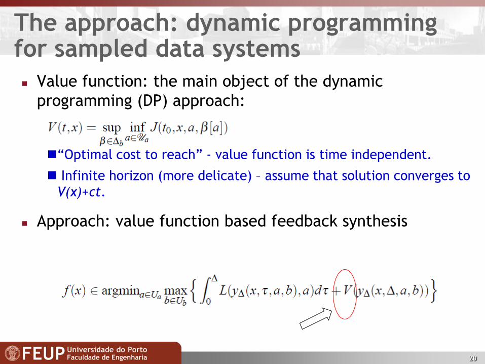
The approach: dynamic programming for sampled data systems

Value function: the main object of the dynamic

programming (DP) approach:

“Optimal cost to reach” - value function is time independent.

Infinite horizon (more delicate) – assume that solution converges to

V(x)+ct.

Approach: value function based feedback synthesis

21

Value function computation

In general, it is not possible to find an analytical expression

for the value function.

• Numerical methods are required.

Numerical computation of the value function is expensive,

but not impossible for systems of low dimension.

• And, for the considered problems, this can be done at the design

stage.

Our solver is based on the semi-Lagrangian (SL) numerical

scheme by Falcone and co-authors, see, e.g.,

22

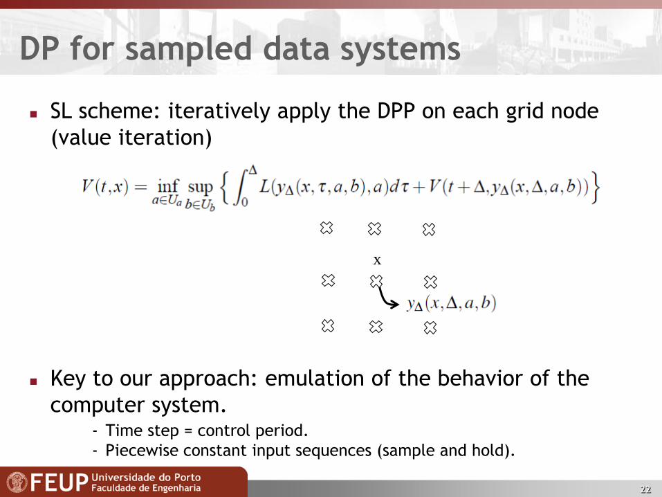
DP for sampled data systems

SL scheme: iteratively apply the DPP on each grid node

(value iteration)

Key to our approach: emulation of the behavior of the

computer system. - Time step = control period.

- Piecewise constant input sequences (sample and hold).

x

23

Implementation of the control law

What to store on the target computer?

• Numerical approximation of the value function

• Constant control on each grid cell

- Requires less computations (local optimization is avoided).

- May require more storage space, depending on the dimension of the

control input.

- In the former approach, the computed control is, in general, closer to

the optimal.

24

Example 1 - Path following model for an AUV

State variables:

• Cross-track error

• Angle relative to path

• Angular velocity

• Fin (angular) position

Input rv defines the path

curvature .

25

Value functions

Specifications

• Maximum cross-track error: 6 m

• Maximum fin angle: 0.26 rad

Inside the MCIS: Infinite horizon problem

• Running cost:

• xmin = -6.000000, -1.570796, -0.400000, -0.260000

• xmax = 6.000000, 1.570796, 0.400000, 0.260000

• nx = 121, 151, 7, 31 (3964807 nodes)

Outside the MCIS: Minimum Time to Reach problem

• xmin = -9.000000, -3.141593, -0.400000

• xmax = 9.000000, 3.141593, 0.400000

• nx = 181, 301, 5 (272405 nodes)

26

Sea trials at Leixões Harbour (2011/07)

28

Final remarks (I)

Further work (not discussed here)

• Refinements/extensions of the numerical solver

- Dealing with the continuous-time nature of the disturbances in the

presence of large sampling steps.

- Input switching costs.

• Aperiodic control

- Next sampling instant decided by the control law.

29

Final remarks (II)

Numerical approximations lead to sub-optimality.

• And also to lack of the robustness: is the adversarial really “doing

its worst”?

• Is this much different from the “approximate dynamic

programming” approaches?

• What “stability” and invariance properties is it possible to assure?

- Verification algorithm based on constrained convex optimization.

- Partition of the state space (e.g., as given by the grid cells).

- Check Lyapunov like decrease condition on each subset, using quadratic

local approximation of the value function.

- Very computationally expensive.

30

Thank you for your attention.

dynamic optimization challenges in autonomous vehicle...

Documents