1

Dynamic Origin-Destination Demand Flow Estimation under Congested Traffic Conditions

Xuesong Zhou

Department of Civil and Environmental Engineering, University of Utah,

Salt Lake City, Utah, 84112, USA. zhou@eng.utah.edu

Chung-Cheng Lu (corresponding author)

Graduate Institute of Information and Logistics Management at National Taipei University of Technology,

Taipei, 106, Taiwan, jasonlu@ntut.edu.tw

Kuilin Zhang

Transportation Research and Analysis Computing Center, Energy Systems Division,

Argonne National Laboratory, Lemont, IL 60439, USA. kzhang@anl.gov

Abstract: This paper presents a single-level nonlinear optimization model to estimate dynamic origin-

destination (OD) demand. A path flow-based optimization model, which incorporates heterogeneous

sources of traffic measurements and does not require explicit dynamic link-path incidences, is developed to

minimize (i) the deviation between observed and estimated traffic states and (ii) the deviation between

aggregated path flows and target OD flows, subject to the dynamic user equilibrium (DUE) constraint

represented by a gap-function-based reformulation. A Lagrangian relaxation modeling framework, which

dualizes the difficult DUE constraint, is proposed and solved by an efficient gradient-projection-based path

flow adjustment algorithm. Additionally, a dynamic network loading (DNL) model, based on Newell’s

simplified kinematic wave theory, is employed in the DUE traffic assignment process to realistically

capture congestion phenomena and shock wave propagation. This study also derives analytical gradient

formulas for the changes in link flow, density and travel time as a function of the unit change of incoming

time-dependent path flow rate in a general network under congestion conditions. Numerical experiments

conducted on three different networks illustrate the effectiveness and shed some light on the properties of

the proposed OD estimation method and the DNL model.

Keywords: OD demand estimation; path flow estimator; Lagrangian relaxation; Newell’s simplified

kinematic wave theory.

2

1. Introduction

Time-dependent origin-destination (OD) demand matrices are fundamental inputs for dynamic traffic

assignment (DTA) models to describe network flow evolution as a result of interactions of individual

travelers. Moreover, many emerging intelligent traffic management applications call for reliable estimates

of dynamic OD demand, in order to generate proactive, coordinated traffic information provision and flow

control strategies based on reliable traffic state estimates. Nevertheless, transportation authorities and

practitioners have long been concerned about the unavailability of high quality time-dependent OD demand

estimates which limits the potential for DTA deployments to analyze and alleviate traffic congestion. In the

past decades, a rich body of literature, to be presented as follows, has been devoted to the methods of

estimating static or time-dependent OD demand tables. However, time-dependent OD demand estimation,

particularly under congested conditions, remains a critical and challenging problem that is attracting

significant attention from transportation researchers to develop theoretically sound and practically

deployable approaches.

1.1 Literature Review

To capture congestion effects in traffic networks, many researchers attempted to integrate equilibrium

assignment into the static OD demand estimation process. Nguyen (1977) and LeBlanc and Farhangian

(1982) incorporated link count observations into a variable demand user equilibrium (UE) assignment

program as equality side-constraints so that the estimated link flows can reproduce observed link counts.

Fisk (1989) combined the maximum entropy model with an UE assignment program to construct a bi-level

mathematical programming problem. Yang et al. (1992) and Florian and Chen (1995) further presented a

more flexible bi-level framework to estimate consistent OD demand, where the upper level is a generalized

least squares (GLS)-based OD estimation model and the lower level is an UE assignment program.

Extending the concepts and solution methodologies of the static OD estimation problem, Cascetta et

al. (1993) proposed a GLS estimator for dynamic OD demand in a general network. A simplified

assignment model was used in their study; that is, path choice fractions are first calculated using a route

choice model and then the resulting path flows are propagated to link flows based on link travel times.

Tavana (2001) proposed a bi-level GLS optimization model and an iterative solution framework to estimate

dynamic OD demand, while seeking to maintain internal consistency between the upper-level demand

estimation problem and the lower-level DTA problem. Along this line, Zhou et al. (2003) and Zhou and

Mahmassani (2006) extended this bi-level dynamic OD estimation approach to utilize multi-day traffic

counts and automated vehicle identification (AVI) data, respectively.

In light of the above review, a typical bi-level dynamic OD demand estimation model needs to solve

iteratively two optimization sub-problems, namely upper-level and lower-level problems. The upper-level

problem is the constrained ordinary/generalized least squares (OLS/GLS) problem, with time-dependent

OD flows as decision variables, which aims to minimize the following two deviation functions: (i) the

deviation between observed and estimated link flows over all time intervals, and (ii) the deviation between

the target or historical demand and estimated demand matrices. The lower-level problem is the UE DTA

problem that determines time-dependent network flow pattern satisfying dynamic user equilibrium (DUE)

conditions. However, it has been widely recognized that, under congested conditions, the mapping between

demand inflow from the origin and link measurements is not a linear relationship as in the static case.

Yang (1995) provided two heuristic solution approaches for solving the general bi-level OD estimation

problem, namely iterative estimation-assignment (IEA) algorithms and sensitivity-analysis based

algorithms (SAB). Tavana (2001) suggested that the IEA algorithm still provides solutions to the Cournot-

Nash game, rather than the Stackelberg game in a bi-level program, because the upper-level optimization

model in IEA does not consider the dependence of link-flow proportions on the OD flows. Based on the

SAB approach, an alternative nonlinear least squares formulation was proposed by Tavana (2001) to

explicitly consider the changes of link flow proportions due to the adjustments in dynamic OD flows, and

numerical derivatives of link flow proportions with respect to OD flows are obtained from a mesoscopic

DTA simulation program (Mahmassani et al. 1994). On the other hand, a standard SAB algorithm needs to

approximate the derivatives through simulation for each OD pair and each time interval in every iteration,

which is computationally intensive, especially for large-scale networks. Recently, Balakrishna et al. (2008)

and Cipriani et al. (2011) introduced gradient approximation methods within a Simultaneous Perturbation

Stochastic Approximation (SPSA) framework, in order to reduce the number of simulation runs for

calculating numerical derivatives or gradients.

Intending to develop an internally consistent approach for the dynamic OD demand estimation

problem, single-level path flow estimators (PFE) have been proposed for the static OD estimation problem,

3

e.g., the linear programming PFE by Sherali et al. (1994) on estimating UE path flows, and the nonlinear

programming PFE by Bell et al. (1997) on estimating stochastic UE path flows. Recently, Nie and Zhang

(2008) formulated a novel single-level formulation based on variational inequalities (VI), which utilizes the

dynamic link-path incidence relationships in a generic projection-based VI solution framework. By

adapting the analytical approach of Ghali and Smith (1995) for evaluating the local link marginal travel

times, Qian and Zhang (2011) further incorporated the travel time gradients into the single-level OD

estimation framework, proposed by Nie and Zhang (2008), in order to utilize travel time measurements,

while linear mappings between OD flow and link flows are still assumed in their upper-level OD estimation

problem. In addition, Nie et al. (2005), Nie and Zhang (2010), and Shen and Wynter (2011) integrated the

integral term in Beckmann’s UE formulation (1956) with the measurement deviations (in terms of the GLS

objective function) to develop alternative single-level path flow formulations for static OD estimation, and

their models can be viewed as a special case of UE assignment with elastic demand.

To fully capture the nonlinear dependency between dynamic OD demand and heterogeneous traffic

measurements, such as link flow, density and travel time, in a general network, it is necessary to

incorporate a reliable dynamic network loading (DNL) component into the OD demand flow estimation

process. The existing DNL methodologies are classified into two major groups: analytic approach and

simulation-based approach. The former includes three types of formulations: mathematical programming,

optimal control and variational inequality, and has the potential for deriving theoretical insights. Earlier

studies (e.g., Merchant and Nemhauser, 1978; Carey, 1987; Friesz et al., 1989) used link/node exit flow

constraints to propagate traffic flows and link performance functions to determine path travel costs. While

using well-defined exit constraints and cost functions makes it possible to establish theoretically the

mathematical properties of solutions (e.g., existence and uniqueness), these analytical models suffer from

several limitations in terms of representing the dynamics and complexity of real-world traffic flow systems,

such as difficulty in ensuring the first-in-first-out (FIFO) queueing discipline and capturing spillback

queues.

In the pioneering works of capturing shock waves and congestion (i.e., queue build-up, spillback and

dissipation), Lighthill and Whitham (1955) and Richards (1956) proposed the kinematic wave (KW) theory,

which rigorously describes traffic flow dynamics by integrating flow conservation constraints, traffic flow

models, and partial differential equations (PDE). Because it is difficult to obtain analytical solutions for

these PDEs, many researchers have presented various finite-difference approximations to solve these

equations numerically. Based on a triangular flow-density relation, Newell proposed a simplified KW

model (1993) to better keep track of shock waves and queue propagation using cumulative flow counts on

links. By discretizing a link into a set of homogeneous unit cells, Daganzo (1994) presented a Cell

Transmission Model (CTM) that adopts a “supply-demand” or “sending-receiving” framework to model

flow dynamics between two successive discretized cells in the link.

1.2 Overview of proposed method

The contributions of this study to the growing body of literature on dynamic OD demand estimation

are as follows.

Instead of working on the commonly-used OD flow variables, this study presents a new path flow-

based optimization model for jointly solving the complex OD demand estimation and UE DTA problems.

Specifically, this model simultaneously minimizes (i) the deviation between measured and estimated traffic

states, and (ii) the deviation between aggregated path flows and target OD flows, subject to a dynamic user

equilibrium (DUE) constraint, which is reformulated using an equivalent gap function. Working in this

path-flow dimension, our formulation can directly aggregate estimated path flows to obtain final OD flow

patterns, and obviate explicit dynamic link-path incidences, as opposed to the majority of previous studies.

By dualizing the difficult DUE constraint into the objective function, this research proposes an

effective Lagrangian relaxation-based solution framework. The relaxed problem can be viewed as a

simultaneous route and departure time user equilibrium (SRDUE) problem with elastic demand, and the

final solution is a set of path flow patterns satisfying “tolled user equilibrium” (Lawphongpanich and Hearn,

2004), where the deviation with respect to traffic measurements can be viewed as an additional penalty for

over-estimated or under-estimated path flows. By incorporating heterogeneous real-world measurements in

the objective function, such as link densities from video surveillance and road side detectors and link travel

times from Bluetooth readings, the proposed estimation model fully utilizes available information to reflect

route choices in a congestion network.

A DNL model that encapsulates Newell’s simplified KW model in a mesoscopic traffic flow

simulation framework is proposed to describe congestion phenomena, such as queues formation, spillback,

4

and dissipation. Explicitly using the cumulative arrival and departure curves, Newell’s traffic flow model

provides a rigorous mathematical formulation to realistically represent traffic dynamics and capture the

impact of shock waves on various macroscopic traffic measures. Compared to standard PDE-based DNL

models that subdivide a long link into segments with a shorter length, Newell’s model can handle

reasonably long links with homogeneous capacity, and its simple form and computational efficiency make

it appealing in developing dynamic OD estimation algorithms.

Based on the proposed DNL model, this research derives analytical, local gradients of different

measurement types, such as link flow, density and travel time, with respect to path flows. This valuable

gradient information not only considers the dependences of link flow/density/travel time changes on the

OD/path flow, but also allows for computing feasible descent directions in an efficient gradient-projection-

based method embedded in the Lagrangian relaxation-based solution framework.

This paper is organized as follows. The single-level path flow estimation framework and the

Lagrangian relaxation-based solution algorithm are delineated in Section 2. Section 3 presents the

underlying mesoscopic DNL model based on Newell’s simplified KW model. Section 4 describes the

derivation of the gradients of typical traffic measurements. Numerical studies on a simple corridor and a

real-world network with time-dependent sensor data are presented in Section 5. Section 6 concludes this

study.

2. Single-level path flow estimation framework

Given sensor data (i.e. observed link flows, densities, and travel times) and target (aggregated

historical) OD demand, the proposed single-level path flow estimation model is a nonlinear optimization

model with path flows as decision variables. Final OD demand estimates can be constructed by summing

up path flows for each OD pair. To construct a tractable single-level nonlinear optimization model, we first

consider the DUE gap function as a side constraint, and then dualize this constraint to the GLS-based

objective function with a Lagrange multiplier. The resulting Lagrangian relaxation model is solved by a

column-generation-based algorithmic framework consisting of a gradient-projection-based descent

direction algorithm for updating path flows, a mesoscopic DNL model for evaluating link and network

performances, and a time-dependent least time path (TDLTP) algorithm for generating paths.

2.1 Notation, assumptions, and problem statement

Variables and notation for the proposed single-level dynamic OD demand estimation framework are

listed as follows.

Set:

A: set of links

S: set of links with sensors, S A

W: set of OD pairs

Hd: set of discretized departure time intervals

Ho: set of discretized observation time intervals

P: set of paths

Index:

t: index of observation time intervals, tHo

τ: index of departure time intervals, τHd

w: index of origin-destination pairs, wW

p: index of paths for each origin-destination pair, pP

a: index of links, aA

m: index of inner loop iterations, m = 1,…, Mmax

n: index of outer loop iterations, n = 1,…, Nmax

Observed measurements:

: observed number of vehicles passing through an upstream detector on link a during observation

interval t

: observed density on link a during observation interval t

: observed travel time of vehicles entering link a during observation interval t

: target demand, which is the total traffic demand for OD pair w over a planning horizon

, , : vectors of observed link flow, density and travel time measurements, respectively

5

: vector of target OD flows for all OD pairs,

Estimated variables and vectors:

q(a, t): estimated number of vehicles passing through an upstream detector on link a during observation

interval t

k(a, t): estimated density on link a during observation interval t

T(a, t): estimated travel time of vehicles entering link a during observation interval t

d(w,): estimated demand for OD pair w during departure time interval τ

r(w,,p): estimated path flow on path p for OD pair w during departure time interval τ

c(w,,p): estimated travel time of vehicles entering the pth

path of OD pair w during departure time interval

τ

(w,): estimated shortest path travel time for OD pair w during departure time interval τ

q, k, T: vectors of estimated link flows, densities and travel times, respectively, for links with sensors

d: vector of OD flows for all OD pairs and departure time intervals, d = {d(w,), w, }

r: vector of estimated path flows for all OD pairs, departure time intervals, and paths, r = {r(w,,p), w, , p}

c: vector of estimated path travel times for all OD pairs, departure time intervals, and paths, c = {c(w,,p),

w, , p}

: vector of estimated least travel times for all OD pairs and departure time intervals, = {(w,), w, }

Functions and thresholds:

,

, : measurement equations for flow, density and link travel time on link a in

time interval t, respectively

f(w,)(r): demand deviation equation between estimated demand and target demand of OD pair w, during

departure time interval

g(r, ): path flow-based gap function

, : convergence thresholds for the gap function and Lagrangian relaxation problems, respectively

Given a transportation network G with a set of nodes and a set of links, the input data include a set of

time-dependent observation data (i.e. flows, densities, and travel times) for a subset of links, S, with sensors

and a set of discretized observation time intervals, Ho, and target OD demand matrices for a set of departure

time intervals, Hd. The time-dependent OD demand estimation problem under consideration aims to find a

vector of path flows r for all OD pairs and departure times such that the resulting estimated network

performance and flow pattern can both match the time-dependent observation data and satisfy DUE

conditions. Thus, the proposed model needs to consider a set of deviation functions for OD demand, link

flows, densities, and travel times, as follows.

(1)

(2)

(3)

(4)

In addition, under the DUE conditions, for each OD pair and departure time interval, no traveler can

improve his/her experienced path travel time by unilaterally changing his/her path, and each traveler is

assigned to a path with the least time-dependent travel time (e.g., Smith, 1993). The DUE conditions are

mathematically formulated as follows.

r(w,, p) [c(w,, p)(w,)] = 0, w, , p, (5)

c(w,, p) (w,) 0, w, , p, (6)

(w,) 0, w, , p, (7)

r(w,, p) 0, w, , p, (8)

pr(w,, p) = d(w,), w, . (9)

Eqs.(5) and (6) are a set of nonlinear complementarity constraints for modeling user equilibrium in the

time-dependent context. For any OD pair w and departure time interval , the travel time for all paths pP,

with positive path flow (i.e. r(w,,p) > 0), is the same and equal to (w,). For any path with zero flow, it has an

6

equal or larger travel time. Eqs.(7) and (8) ensure the non-negativity of both path flow and least travel

times. Eq.(9) maintains the OD demand and path flow balance.

The above DUE conditions can be reformulated as a nonlinear complementarity problem (NCP) by

extending the NCP formulation of the static user equilibrium problem, proposed by Aashtiani and Magnanti

(1981), to the dynamic case. Alternatively, they can also be formulated as a variational inequality problem

(VIP), e.g., Smith (1993). In this study, we reformulate the DUE conditions using an equivalent gap

function as in Eq.(10), which was proposed by Lu et al. (2009) as an extension of a gap function

formulation for static user equilibrium, developed by Lo and Chen (2000).

g(r, ) = wp{r(w,,p)[c(w,,p)(w,)]}. (10)

Note that, by definition, g(r, ) 0.

2.2 Nonlinear programming formulations

By re-defining the above-mentioned deviation functions, Eqs.(1)-(4), at the network level, as follows,

, (11)

, (12)

, (13)

, (14)

We are now ready to present a mathematical program with complementarity constraints (MPCC) for the

time-dependent OD demand estimation problem with multiple types of observations in the following.

P1: mathematical program with complementarity constraints

Min z(r) = d f(r) + q hq(r) + k h

k(r) + T h

T(r) (15)

s.t. Eqs.(5)-(8),

where d, q, k, and T are the weights reflecting different degrees of confidence on target OD demand,

and (observed) link flows, densities, and travel times, respectively. In a GLS framework, those weights can

be viewed as the inverses of the variances of the distinct sources of measurements. In the proposed path-

based formulation, OD demand d(w,) in Eq.(1) is substituted by its corresponding time-dependent path

flows, so the path flow balance constraints, Eq.(9), are not included in P1. However, this MPCC is still

difficult to be solved due to the nonlinear complementarity constraints in Eq.(5), which may not satisfy the

requirement of constraint qualifications. As mentioned previously, instead of solving directly the MPCC,

P1, the nonlinear complementarity constraints, Eq.(5), are replaced by the equivalent gap function-based

constraint, in Eq.(16).

g(r, ) , (16)

where is a sufficiently small positive threshold, close to zero. This reformulation can be viewed as an

application of the regularization technique to approximate the MPCCs (Interested readers are referred to

Scholters 2001). The gap-function-based reformulation of P1 is presented as follows.

P2: gap-function-based reformulation of P1

Min z(r) = d f(r) + q hq(r) + k h

k(r) + T h

T(r) (17)

s.t. Eqs.(6)-(8) and (16).

Note that similar to the solution uniqueness property of static traffic assignment problems, the proposed

model may have multiple path flow solutions corresponding to the same equilibrium link flow pattern. We

shall bear in mind that the properties of solution existence and uniqueness need to be further studied for this

formulation; these issues are not discussed in the current paper.

2.3 Solution Procedure

To efficiently solve P2, a Lagrangian relaxation reformulation, P3, is constructed by dualizing the

(hard) gap-function-based constraint, Eq.(16), to the objective function, with a (non-negative) Lagrange

multiplier . Thus, in this reformulation, we only need to handle a set of easy constraints, Eqs.(6)-(8).

P3: Lagrangian relaxation reformulation of P2

Minr, , L(r, , ) = z(r) + [g(r, ) ]

= d f(r) + q hq(r) + k h

k(r) + T h

T(r) + [g(r, ) ] (18)

s.t. Eqs.(6)-(8) and 0.

For a given Lagrange multiplier , P3 is reduced to a Lagrangian lower bound problem to which the

optimal solution provides a lower bound to the problem P2. Thus, solving P3 involves the identification of

the optimal value of that produces the tightest (or largest) lower bound to the primal problem P2. The

resulting problem is called the Lagrangian dual problem, P4 (e.g., Bazara’a et al., 1993). According to the

strong duality theorem (e.g., Theorem 6.2.4 in Bazara’a et al., 1993), the optimal objective value of P4 is

7

identical to that of the original problem, P2, if some constraint qualifications hold true; otherwise, there is a

duality gap.

P4: Lagrangian dual problem

Max0 {LD() = inf{z(r) + [g(r, ) ]}} (19)

Within this Lagrangian relaxation and duality framework, in each outer loop iteration n, the solution

procedure for problem P2 consists of two major algorithmic steps: (i) given a Lagrange multiplier (n), find

an optimal path flow vector by solving the Lagrangian lower bound problem, P5, and (ii) given a path flow

vector r(n)

and least travel time vector (n), update the Lagrange multiplier (n+1)

by using the subgradient

optimization method.

According to Theorems 6.3.1 and 6.3.4 in Bazara’a et al. (1993), the objective function, LD(), is

concave and sub-differentiable; that is, it has a subgradient. Specifically, the following updating method is

adopted to determine the Lagrange multiplier (n+1) using the subgradient of (n)

, g(r(n)

, (n)) .

(n+1) = max{0, (n)

+ (n)[g(r

(n), (n)

) ]}, (20)

where (n) is the step size for updating the Lagrange multiplier (e.g., Bertsekas, 1995).

P5: Lagrangian lower bound problem

Min {L(r, ) = z(r) + (n)[g(r, ) ]} (21)

s.t. constraints (6)-(8).

For a given set of feasible paths for all OD pairs and Lagrange multiplier (n), in the inner loop for solving

the Lagrangian lower bound problem, P5, the set of time-dependent least time paths can be identified in a

reduced solution space. Hence, the inequality constraints in Eq.(6) and non-negative constraints in Eq.(7)

for least path travel times can be replaced by Eq.(22).

(22)

Recall that m is the index of inner loop iterations. In addition, to maintain the feasibility of the non-

negativity constraints in Eq.(8), a projection approach can be used to project the solution to the non-

negative solution space (e.g., Lu et al., 2009). As a result, we can update path flows by a gradient-

projection-based descent direction method in the reduced solution space, as shown in Eq.(23).

(23)

where (m) is the step size for updating path flows in the (restricted) Lagrangian lower bound problem, P5.

The gradients which consist of the first-order partial derivatives with respect to a path flow variable r(w,,p)

can be derived as follows.

(24)

(25)

(26)

(27)

(28)

Estimated link flows, densities, and link/path travel times and the corresponding partial derivatives, namely

hq(r), h

k(r),h

T(r) and c(w,, p)(r)/r(w,, p) can be obtained from a DNL model, such as the CTM

(Daganzo, 1994), DYNASMART (Mahmassani et al.1994), or the proposed DNL model based on Newells’

simplified KW model, to be detailed in the next section.

The detailed algorithmic steps of solving the Lagrangian relaxation reformulation, P3, are presented as

follows, with a flow chart depicted in Fig. 1. The basic idea is to iteratively solve the Lagrangian lower

bound problem, P5, using the gradient-projection-based descent direction method (i.e., Eq.(23)), and update

the Lagrange multiplier using Eq.(20), until reaching an optimal path flow vector that can both fit the

time-varying observation data and satisfy the DUE conditions (i.e., minimize the gap function). To

circumvent the difficulty of path enumeration, the time-dependent least time path (TDLTP) algorithm,

developed by Ziliaskouplas and Mahmassani (1993), is employed to generate new paths in each outer loop

iteration n.

8

Algorithm 1: Time-dependent path flow estimation method

Step 1: Initialization

Step 1.1: Set iteration counter n = 0. Input a historical demand table, , w, its corresponding

temporal distribution profile, and time-dependent link measurements (densities, flows, and travel

times).

Step 1.2: Perform DUE traffic assignment with a time-dependent OD demand matrix, d(n)

, based on

, w, and the temporal profile, to build a feasible path .

Step 1.3: According to the assignment results (i.e., estimated link densities, flows, and travel times),

compute the upper bound of the optimal solution to the primal problem P2 as follows:

zUB

= q hq(r

(n)) + k h

k(r

(n)) + T h

T(r

(n)). (29)

Note that f(r(n)

) = 0, as the DUE assignment loads the target demands , w, and satisfy g(r(n)

,

(n)) = 0.

Step 1.4: Initialize (n) to a positive value, such as 1.0.

Step 2: Solve the Lagrangian lower bound problem, P5, to find the optimal path flows corresponding to

(n).

Step 2.1: Set iteration counter m = 0. Read estimated link flows, densities, travel times, path flows, path

travel times and corresponding gradients f(r), hq(r), h

k(r) and h

T(r) from the previous outer

iteration n.

Step 2.2: Identify the least time paths and determine

, according to Eq.(22) .

Step 2.3: Calculate the gradient of the gap function, g(r(m)

, (m)), according to Eq.(28).

Step 2.4: Determine flow updating step size (m) according to a diminishing step size rule, such as the

Method of Successive Averages (MSA), i.e. (m) = 1/(m+1).

Step 2.5: Update path flows

, according to Eq.(23).

Step2.6: Dynamic network loading. Load path flow assignment r(m+1)

to the DNL model, to be presented

in Section 3, to obtain estimated link densities, flows, and travel times.

Step 2.7: Convergence checking for the (inner) Lagrangian lower bound problem, P5. Update the

objective function, L(r(m)

, (m), (n)

). If m < Mmax or L(r(m)

, (m), (n)

) is improved, then m = m+1, and

go to Step 2.2; otherwise, go to Step 2.8.

Step 2.8: Update the tightest lower bound, zLB

, to the primal problem P2, as the following:

zLB

= Max{zLB

, d f(r(m)

)+q hq(r

(m))+k h

k(r

(m))+T h

T(r

(m))+ (n)

g(r(m)

, (m))}. (30)

Step 3: Update the upper bound

Step 3.1: Construct a time-dependent OD demand matrix by summing up the time-dependent path

flows for each O-D pair and each departure time obtained from the solution of the Lagrangian lower

bound problem.

d(w,) = pP r(w, , p), w, . (31)

Step 3.2: Perform DUE traffic assignment for the constructed OD demand matrix d = {d(w,), w, }.

According to the assignment results (i.e., estimated link densities, flows, and travel times), obtain

the equilibrium path flows and update the tightest upper bound as:

zUB

= Min{zUB

, q hq(r

(n)) + k h

k(r

(n)) + T h

T(r

(n))}. (32)

Step 4: Convergence checking.

If n > Nmax or zUB

zLB

< , then stop; otherwise, set n = n + 1, and go to Step 4.

Step 5: Update Lagrange multiplier

Step 5.1: Obtain estimated link flows, path flows, and path travel times from the last iteration of Step 2

(i.e., solving P5). Update the gap value, g(r(n)

, (n)), using these estimates.

Step 5.2: Determine the step size, (n), by a diminishing step size rule, such as MSA, i.e. (n)

= 1/(n+1).

Step 5.3: Update Lagrange multiplier, (n+1), according to Eq.(20). Go to Step 5.

Step 6: Path generation. Compute least time path for each departure time and OD pair using the TDLTP

algorithm and add newly generated paths to the feasible path set . Return to Step 2.

There is an additional remark about the lower bound and upper bound solutions obtained by the

proposed algorithm. Because the lower bound problem P5 is not convex, the iterative path flow adjusting

process in Step 2 might not converge to an optimal solution, within a limited number of iterations. In this

case, the objective value of L(r, ) in Eq.(21) is greater than the minimum/optimum objective value. As a

9

result, the solution gap between the upper and lower bound solutions, i.e., zUB

zLB

, may be underestimated

and the final, attainable solution quality may be overestimated. However, it should be recognized that, in

addition to estimating the solution gap, a more important task of the proposed Lagrangian relaxation

procedure is to obtain a better upper bound zUB

and the corresponding demand matrix D = {d(w,), w, } to

the original problem P1. Essentially, in each iteration of the algorithm, we first obtain a better path flow

solution by solving the lower bound problem P5, and then construct and evaluate feasible demand flow

solution, d(w,) = pPr(w, , p), w, , in order to progressively find a solution with the assigned flow

pattern that minimizes the overall measurement deviations.

10

Fig. 1 Flowchart of the time-dependent path flow estimation algorithm

3. Dynamic network loading (DNL) model

Given travelers' choices of departure times and routes, the DNL model is employed to describe

network traffic flow dynamic evolution and to obtain the corresponding network performance statistics,

such as link flow and/or path travel times. The following notation is used in presenting the DNL model.

Set:

A: set of links

S: set of links with sensors, S A

W: set of OD pairs

Hd: set of discretized departure time intervals

Ho: set of discretized observation time intervals

P: set of paths

No

Yes

Step 1. Initialization

Input data and initialize

iteration counter n and

Lagrange multiplier

Step 2. Solve the Lagrangian lower bound problem, P5, to find the

optimal path flows corresponding to the current Lagrange multiplier.

Update the tightest lower bound to the primal problem P2 as: zLB

=

Max{zLB

, d f(r(m)

) +q hq(r

(m)) + k h

k(r

(m)) + T h

T(r

(m)) + (n)

g(r(m)

,

(m))}.

Step 4. Convergence

checking for solving

problem P3: if zUBz

LB < ,

or n > Nmax ?

Step 5. Update Lagrange multiplier (n) according to Eq. (20).

Step 6. Generate new path using the TDLTP algorithm.

Stop; output

demand matrix D

= {d(w,), w, }

with the best zUB

Step 3. Construct demand flow matrix through d(w,) = pPr(w, , p),

w, , and perform a DUE traffic assignment for the constructed OD

demand matrix. According to the assignment results, update zUB

=

Min{zUB

, q hq(r

(n)) + k h

k(r

(n)) + T h

T(r

(n))}.

11

Index:

t: index of simulation time intervals

τ: index of departure time intervals

w: index of origin-destination pairs

p: index of paths for each origin-destination pair; that is, the pth

path departing at time t for origin-

destination pair w

j: global path index that represents a combination of (w, p, t)

l: link sequence number on a path, l = 1,…, L(j), where, L(j) is the number of links on path j

a, b: index of links

Input Parameters:

length(a): length of link a

nlanes(a): number of lanes of link a

kjam(a): jam density on link a

nmax

(a): number of vehicles that can be stored on link a, nmax

(a) = kjam nlanes(a) length(a)

vf(a): free-flow speed on link a

wb(a): backward wave speed on link a

FFTT(a): free-flow travel time on link a, FFTT(a) = length(a) / vf(a)

BWTT(a): backward wave travel time on link a, BWTT(a) = length(a) / wb(a)

qmax

(a, t): maximal discharge rate of link a at simulation time t

β(j, l) : link index for the lth

link on path j

d(w,): OD demand flow from origin pair w at departure time IL(b): set of incoming links merging into link b

Variables:

r(j): route flow on the pth

path oforigin-destination pair w departing time t, i.e. r(j) = r(w,p,t)

A(j, a, t): cumulative number of vehicles on path j arriving at the upstream node of link a and ready to

move into link a at time t

V(j, a, t): cumulative number of vehicles on path j waiting at the vertical queue of the downstream node

of link a at time t

D(j, a, t): cumulative actual number of vehicles on path j departing from the downstream node of link a

(i.e. moving out of link a from the downstream node of link a) at time t

A(a, t): cumulative number of vehicles arriving at the upstream node of link a and ready to move into

link a at time t

V(a, t): cumulative number of vehicles waiting at the vertical queue of the downstream node of link a at

time t

D(a, t): cumulative actual number of vehicles departing from the downstream node of link a (i.e.

moving out of link a from the downstream node of link a) at time t.

q(a, t): the number of vehicles leaving link a at time t

n(a, t): the number of vehicles on link a at time t

k(a, t): density of link a at time t

capout

(a, t): outflow capacity of link a at time t

capin

(a, t): inflow capacity of link a at time t

3.1. Newell’s simplified kinematic wave model

The first-order model, a classical macroscopic traffic flow model developed by Lighthilland and

Whitham (1955) and Richards (1956), describes traffic flow using three basic equations: the fundamental

diagram of flow-density relationship, the flow conservation law, and an equilibrium flow-density

relationship.

(33)

where is the source term or net vehicle generation rate. The conservation law can be derived from

an analogy between traffic flow and a one-dimensional compressible fluid. Newell’s simplified kinematic

wave (KW) model (1993) is built upon an assumption of a triangular flow-density relationship. This study

aims to incorporate Newell’s KW model to describe traffic congestion propagation realistically, such as

phenomena of queue build-up, spillback, and dissipation, in a road traffic network. As shown in Fig. 2,

12

Newell’s model is concerned about three state variables on each link a: (i) cumulative flow count A(a, t) for

vehicles moving into link a through the upstream node, (ii) cumulative flow count V(a, t) for vehicles

waiting at the vertical queue of the downstream node of link a at time t, and (iii) cumulative flow count D(a,

t) for vehicles moving out of link a through the downstream node.

Cumulative

flow count

t'

A V

DFFTT

t'+FFTT t-BWTT t

dN

=K

jam×

leng

th×

nla

nes

TimeBWTT

Amax

Fig. 2 Illustration of cumulative arrival and departure curves A(t) and D(t), and the shifted arrival curve V(t)

In the following, we adopt Hurdle and Son’s framework (2000) to explain how Newell’s model is able

to model forward and backward waves using the cumulative flow counts. Let x be the location along the

corridor, and N(x, t) the cumulative flow count at location x and time t of a link. The change of N(x, t) along

a characteristic line (wave) is represented as follows.

. (34)

A wave represents the propagation of a change in flow and density along the roadway, and the wave speed

is the slope of the characteristics line:

. (35)

Along the movement of a wave, we substitute

into Eq.(34), so that we can link the difference of

cumulative flow counts together through

. (36)

For the triangular shaped flow-density relation with constant forward and backward wave speeds, it is

easy to verify that, when the speed of the forward wave is , the general cumulative flow count updating

formula, Eq.(36), reduces to

. (37)

Under congested traffic conditions with a constant backward wave speed , we have

. (38)

and Eq. (36) can be rewritten as

. (39)

Eq.(39) is used to describe how a backward wave travels through the link. As shown in Fig. 2, when a

queue spills back from the downstream to the upstream, the arrival and departure cumulative flow counts at

two ends of a link (at timestamps t and time tBWTT(a)) need to ensure a constant difference of dN = kjam(a)

length(a) nlanes(a), and the capacity restriction is propagated throughout the link using a time duration

of BWTT(a) = length(a) / wb(a).

13

3.2. Traffic flow dynamics constraints and states updating

To describe traffic flow dynamics constraints in a DTA model with multiple OD pairs and paths, one

key modeling challenge is to map path flow variables to link-based cumulative flow variables used in

Newell’s KW model. Recall that, the path flows are the decision variables in the proposed dynamic OD

demand flow estimation model. This sub-section first defines a set of link, path and demand flow balance

constraints, and then describes the constraints for capturing shockwave propagation at lane drop, merge and

diverge bottlenecks.

We first define the demand flow balance constraint for each (w,) pair over its path set as follows.

w,(t,)=1, (40)

where (t,) = 1 indicates that (simulation) time interval t is inside departure time interval . Then, the

DNL needs to load the path flow, r(j), to the first link of each time-dependent path j, where r(j) correponds

to r(w, p, t), the flow on the pth

path of OD pair w leaving at time t.

. (41)

Cumulative flow counts are moved from the beginning of link a to its vertical queue for each time-

dependent path j

. (42)

The cumulative departure flow count can be transfered from a curent link β(j,l) to the cumulative arrival

count on the next link β(j,l+1) along the path j,

. (43)

By summing up all cumulative arrival and departure flows across diffent paths, we can obtain cumulative

link arrival and departure flows as follows.

. (44)

. (45)

When vehicles are discharged from the queue, Eq.(46) is used to satisfy the outflow capacity constraints

and capture the effect of queue spillback.

. (46)

In Eq.(46), is the number of vehicles waiting at the vertical queue of link a at

time t. If intersection or freeway control elements (e.g., signals and ramp meters) are included, time-

dependent maximum queue discharge rate qmax

(a, t) can be modified according to different circumstances

and scenarios.

a2

b

c1

c2

a1

a b c

Fig. 3 Simple networks; left: lane drop; right: merge and diverge

To illustrate how to calculate capout

(a, t) in Eq.(46) through backward wave propagation, the following

discussion considers a sequential corridor along links a, b and c, where the traffic congestion from the lane

drop bottleneck on link c has spilled back to link b and is now propagated to the middle of link a, as shown

in the left portion of Fig. 3. Obviously, under congested conditions, maximum outflow capacity

on the link b is determined by the bottleneck inflow rate ofbottleneck c.

. (47)

The right portion of Fig. 3 depicts a merge junction with incoming links a1 and a2 merging into

downstream link b. In this study, the available outflow capacity of an incoming link, say a1 in Fig. 3, is

assumed to be proportional to the number of lanes on that link. That is,

. (48)

For diverge junctions, one thorny issue in macroscopic fluid-based DNL models is to determine the

proportions of vehicular flow (toward different destinations) moving out from link b to its outgoing links.

Within a mesoscopic DNL model (Mahmassani, 2001), each vehicle carries its own OD and path

information, so the outflow (destination) proportions from a link are indirectly determined by the path

attributes associated with vehicles waiting at that link’s vertical queue. In this study, the vertical queue is

implemented as a first-in-first-out (FIFO) queue, so the proposed DNL model strictly satisfies the FIFO

14

constraint. If a vehicle in the front of the vertical queue is blocked, due to unavailable outflow capacity of a

downstream link, then the vehicles behind in the queue will be also blocked. For example, in Fig. 3, for a

vehicle going from link b to link c1, if has been consumed by the previous vehicles in the

vertical queue, then this vehicle will not be able to move to link c1 and all the vehicles behind that vehicle

in the queue cannot move either, even though they head to link c2. Note that, to model complex geometric

features, such as left-turn bays on multi-lane links, we need to decompose a link into multiple connected

cells, with each cell satisfying the FIFO constraint.

Considering the fully congested link b in Fig. 4, the inflow capacity at time t is in turn determined by

the outflow capacity capout

(b, tBWTT) at time tBWTT. The inflow capacity capin

(b, t) is defined in terms

of the difference of the cumulative arrival flow counts between two consecutive time stamps t1 and t as

follows,

. (49)

Applying the backward wave propagation constraint, Eq.(39), to the cumulative flow counts at the

upstream end (i.e. arrival count) and downstream end (i.e. departure count) of link b leads to

. (50)

Finally, we are ready to compute outflow capacity for link a, and the

corresponding cumulative departure flow curve at time t through Eq.(46).

Cumulative

flow count

t-1 t

Time

Amax(t)

A(t-1)capin(t)

Time

t-BWTT-1t-BWTT

D(t-BWTT)

D(t-BWTT-1)

capout(t-BWTT)

A

V

D

Fig. 4 Illustration of queue spillback and propagation of outgoing flow constraint from the downstream end

at time tBWTT to the upstream end at time t

The space-time plot in

Fig. 5 further demonstrates how Newell’s model uses cumulative counts to model the forward and

backward waves in describing queue phenomenon on links a and b. Exactly at time t1, the tail of the

queue at the downstream link b propagates to its upstream node. That is, if the cumulative outflow count at

a lagged time stamp t BWTT(b) 1 on link b equals to the cumulative inflow count at time t1, then a

queue spillback occurs as a backward wave is able to propagate through the congested time-space “mass”

of the link. Compared to the conventional vertical queue model, where the inflow rate of a link is not

constrained by the available physical length, the inflow rate in Newell’s model is governed by the discharge

flow of a link through the backward wave propagation process. Furthermore the number of vehicles on a

lane should not be greater than kjamlength(b). As a result, the proposed model is able to detect and capture

queue spillbacks to upstream link(s).

15

Time axis

shock wave

backward w

ave

( )( )

b

length bBWTT b

w

forw

ard w

ave

( )( )

f

length aFFTT a

v

Time t-1

shoc

k w

ave

Spac

e ax

is

Link b

Link a

A(b,t-1)

D(b,t-BWTT(b)-1)

N max

(b)

Fig. 5 Illustration of forward and backward wave representation in Newell’s simplified kinematic model

4. Evaluation of partial derivatives with respect to path flow perturbation

Solving the proposed single-level dynamic OD estimation model requires the evaluation of the partial

derivatives with respect to time-varying path flows, i.e.,

,

,

, and

in

Eqs.(25)-(28), These partial derivatives represent the marginal effects of an additional unit of path inflow

on link (i.e., link flow, density, and travel time) and path performances (i.e., path travel time). This section

delineates the evaluation of these partial derivatives due to path flow perturbation in a congested network,

based on the results of the DNL model (i.e., cumulative link inflow and outflow curves), presented in

Section 3. The following notation is used throughout this section.

L : the number of links on the path

l: link index l=1, 2, …L

: the time when an additional unit of perturbation flow arrives at link l

: the time when an additional unit of perturbation flow departs from link l

: the time when the queue starts to form on link l

: the time when the queue vanishes on link l

:

: the time when the queue on link l starts to spillback to its upstream link l1

: cumulative arrivals at time

: cumulative arrivals at time

4.1 Evaluation of link partial derivatives on a congested link

In this study, the link partial derivative is referred to as the change in link flow, density, or travel time,

due to an additional unit of link/path inflow. For instance, the link travel time derivative is the travel time

contribution of an additional unit of vehicular flow on link l at time to the link travel time , where

is in time interval t. In their pioneering work, Ghali and Smith (1995) presented an analytical approach to

evaluate the (local) link marginal travel time (or delay) on a congested link, based on link cumulative flow

curves. An illustration of the approach is depicted in Fig. 6. In the figure, the two solid lines represent the

cumulative arrival and departure curves, while the dashed line represents the cumulative vertical queue.

The (outflow) capacity of the link is c. The key result of their approach is that the link marginal delay

equals the grey area.

16

Fig. 6 Illustration of link marginal delay on a congested link

(For example, the queue starts at

= 7:00 AM, an additional unit of vehicle, n'= 1000, enters link l at time

= 7:10AM, leaves the link at time

= 7:50AM, the queue dissipates on link l at = 8:30AM, and

=

8:15AM, assuming FFTT(l) = 15 min.)

The following propositions can be induced from Fig. 6 for deriving the marginal effects on link flow

(inflow and outflow), density, and travel time.

Proposition 1: Under free-flow conditions, an extra unit of flow arriving at the upstream end of link l at

time results in the following: (i) the link inflow and outflow increase by 1 at times

and , respectively,

and the flow rates at the other time intervals do not change; (ii) the link density increases by 1 from to

;

(iii) the individual travel times are not changed, and

.

Proposition 2: Under partially congested conditions and constant link (outflow) capacity c, an extra unit of

flow arriving at the upstream end of link l at time results in the following: (i) the link inflow and outflow

increase by 1 at times and

, respectively, and the flow rates at the other time intervals do not change; (ii)

the link density increases by 1 from to

; (iii) the flows arriving between and

experience the

additional delay 1/c, because it takes 1/c to discharge this perturbation flow.

Proposition 3: If the perturbation flow arrives at the upstream end of link when it is fully congested, then

the link flow and density will remain the same at the maximum flow rate, respectively, and then increase by

1 when the link becomes partially congested.

With the proposed DNL model based on Newell’s simplified KW model, we can adapt Eq.(39) to

detect if the queue spills back to the upstream end of link l using the following equation.

. (51)

Specifically, if the above strict inequality holds, then the queue has not propagated back to the upstream

end of the link (or the link is partially congested). Otherwise, the link is fully congested; the queue

propagates throughout the link along the backward wave line, as illustrated in Fig. 5. Note, that, under fully

congested conditions, the prevailing link density k(l) at time t might be smaller than kjam(l).

A common pitfall for deriving the partial derivative of link density, under congested conditions, is to

record the increase in density by 1 from to

(e.g., from 7:10AM to 7:50AM with the duration of 40-min

in Fig. 6). Proposition 2, induced from Fig. 6, clarifies that the actual change in link density would last until

the queue vanishes at time , so the change in link density should cover a duration of 80-min from

7:10AM to 8:30AM in our example. Proposition 2 also indicates that the change in link outflow, due to an

extra unit of flow arriving under congested conditions, occurs at the time (e.g. 8:30AM), rather than

(e.g., 7:50AM). Note that, by multiplying the (individual) extra delay, 1/c, by the number of vehicles

arriving between and

(i.e., ), we can obtain that, if is between

and

, the local link

marginal delay is equal to

, which is the sum of the traversal time of the perturbation flow,

,

and the additional delay imposed by the perturbation on others is equal to

. This evaluation

approach for link marginal travel times was also adopted by, for instance, Levinson (2002), Shen et al.

(2007), and Qian and Zhang (2011) in the context of system optimal traffic assignment.

4.2 Evaluation of the impact of path flow perturbation on two sequential links

In static transportation networks, the path travel time marginal, which is the partial derivative of the

c FFTT(l)

A

V(t)

)

A

One

unit of

flow

nA

D(t)

)

A

A(t)

)

A

N

Link marginal delay equals this area,

which equals this grey area

17

total system-wide travel time, can be obtained as the sum of the link marginals of a path’s constituent links.

However, in dynamic and congested transportation networks, this additivity assumption may lead to a

severe deficiency in the evaluation of path marginals, as indicated by Shen et al. (2007), who showed that it

is necessary to explicitly trace the propagation of path flow perturbation in evaluating path marginal travel

times and proposed an evaluation method of path marginals. Thus, this study evaluates the impact of path

flow perturbation (i.e., the partial derivatives) in the individual link-time level by tracing the changes in

link flow, link density, and link travel time on a sequence of links (i.e., a path) and over different time

intervals, due to the addition of unit flow to a path. Qian and Zhang (2011) conducted a similar analysis for

individual path marginal travel times.

Firstly, consider a freeway or an arterial segment with two sequential links, without merges and

diverges, say link l1 and link l. Under congested conditions, there are three basic cases of interest, when

the additional unit of flow arrives at this segment.

(i) There is a bottleneck on the downstream link l and the queue on link l does not spill back to link

l1; that is, link l1 is in free-flow condition while link l is partially congested.

(ii) There is a bottleneck on the downstream link l and the queue on link l spills back to link l1; that

is, link l1 is partially congested while link l is fully congested.

(iii) There is a bottleneck on each of the two links, and the two bottlenecks are independent, assuming

that both links are sufficiently long so that the queue in the downstream does not spill back to the upstream.

This is in fact the case in which both links l1 and l are partially congested.

For cases (i) and (iii), Proposition 2 can be applied to determine the marginal effects of the additional unit

of flow on link flow, density, and travel time. For case (ii), there are two possible scenarios. As depicted in

Fig. 7(a), one scenario is that the additional unit of flow does not encounter the queue on link l1, so it can

enter link l at time

, when link l is partially congested, i.e.,

or

. Another scenario, as depicted in Fig. 7(b), is that the perturbation flow encounters the queue on

link l1, i.e.

, so it cannot enter link l until time

. Note

that

, the time at which the queue on link l start to spill back to link l1. While it is possible to

detect that the queue spills back based on Eq.(51), tracing the propagation of the perturbation flow in the

case of queue spillback is still very difficult, as also indicated by, for instance, Shen et al. (2007) and Qian

and Zhang (2011). In order to strike a balance between computational efficiency and numerical accuracy,

this study applies Proposition 3 to the analysis of link marginal effects on the current link l under fully

congested states, and does not trace back the flow perturbation from link l to link l1.

Fig. 7 Link marginal analysis for the case of queue spillback

Next, we discuss the evaluation of partial derivatives of two sequential links in merge or diverge

junctions, using the illustrative network depicted in Fig. 3. Assume that link b is sufficiently long or

consists of several links, so the two junctions are distantly separated. The additional perturbation flow goes

through links a1, b, and c1 in order. In the merge junction, as described in Section 3, the inflow capacity of

vehicle trajectory

+FFTT(l1) vehicle trajectory

Time axis Time axis

Sp

ace

axis

Link l

Link l1

(a) (b)

=

=

=

=

=

18

link b is assumed to be distributed according to the number of lanes of the incoming links (i.e., links a1 and

a2), so the perturbation flow from link a1 to link b does not affect the travel time, density, and flow on link

a2. Therefore, the analysis results presented above for two sequential links (i.e., Cases (i), (ii), and (iii)) can

be directly employed to determine the path marginal effects of flow, density, and travel time.

When the perturbation flow arrives at the diverge junction, if there is a bottleneck active on link c1 or

a bottleneck active on each of the two links, b and c1, the results discussed above for two sequential links

can be applied to evaluate the path marginal effects of interest. Besides, a bottleneck active on link c2 will

not affect the evaluation of the path derivatives on links b and c1, unless the queue on link c2 spills back to

link b. In this case (i.e., there is no inflow capacity on link c2 to accommodate the incoming flow), due to

the FIFO constraint described in Section 3, the perturbation flow cannot enter link c1 until the vehicles in

front of it in the vertical queue of link b get discharged. We may consider this case as there is a bottleneck

at the downstream end of link b, and adopt the results in Proposition 2 to determine the link/path partial

derivatives.

Lastly, we illustrate the evaluation of the partial derivative of path travel time with respect to an unit of

additional flow in the same time interval, i.e.,

in Eq.(28), based on the case of two partially

congested links (i.e., case (iii)), depicted in Fig. 8. Note that the analysis result can be applied to the other

two cases (i and ii). Let link l1 be the first (congested) link of a path under evaluation. Consider a vehicle

veh that enters link l1 at time and leaves at time

. According to Proposition 2, the extra delay

experienced by this vehicle on link l1 is 1/c, due to the perturbation flow entering the link in the same

time interval, where c is the capacity of link l1. Then, veh enters link l at time and leaves at time

,

but the impact of path flow perturbation on link l occurs at a later time stamp

.

Because

refers to the marginal effect of the perturbation flow on the path travel time, , of

vehicle veh, is affected by the perturbation flow only on link l1. The perturbation flow, which

departs in the same time interval as vehicle veh, will not affect the travel time of veh after link l1.

Therefore, the partial derivative

.

Fig. 8 Illustration of the scenario with two partially congested links

4.3 Computational method for evaluating partial derivatives due to path flow propagation

Based on the above analyses, we now present Algorithm 2, which traces the propagation of an

additional unit of flow and calculates the gradients in Eqs.(25)-(27) of a given path at departure time . Let

and

be the starting and end times of (event) impact period on link l, respectively. Under the event-

based mesoscopic traffic simulation framework, described in Section 3.2, can take on one of the three

values: ,

, or

, corresponding to the free-flow condition, congested without queue

spillback (or partially congested), and congested with queue spillback (or fully congested), respectively.

Algorithm 2: Computational method for path marginals

Initialize link entry time = departure time , and link index l = 1.

One unit

c

One unit V(t)

)

A

V(t)

)

A

D(t)

)

A

A(t)

)

A

N

Link l1

D(t)

)

A

A(t)

)

A

N

Link l

19

Do while link index l ≤ L

Given , determine the end time of impact period

as follows.

Step 1: Set the tentative entrance time to the vertical queue

.

Step 2: (Determining the current condition)

Step 2.1: If there is no vertical queue at time

and

is not equal to the beginning of the

queue (

), then the perturbation flow enters link l under uncongested conditions: perform

Step 3; otherwise, time

is under congested conditions.

Step 2.2: Next, if there is no queue spillback between time and

, then perform

Step 4; otherwise, perform Step 5.

Step 3: (Free-flow condition)

Step 3.1:

.

Step 3.2: Update link inflow, outflow and travel time partial derivatives according to Proposition 1.

Step 3.3: If link l has the measurements (e.g., , , and ), then cumulate hq(r), h

k(r) and

hT(r), according to Eqs.(25)-(27).

Step 3.4: Set l = l+1 and

.

Step 4: (Congested condition without queue spillback)

Step 4.1: Set

.

Step 4.2: Update link partial derivatives according to Proposition 2 for impact period [ ,

].

Step 4.3: If link l has the measurements (e.g., , , and ), then cumulate hq(r), h

k(r) and

hT(r), according to Eqs.(25)-(27).

Step 4.4: Set l= l+1 and

.

Step 5 (Congested condition with queue spillback):

Step 5.1: Find the queue spillback time (in terms of link entrance time)

, and set

.

Step 5.2: Update link partial derivatives according to Proposition 3 for impact period [ ,

].

Step 5.3: If link l has the measurements (e.g., , , and ), then cumulate hq(r), h

k(r) and

hT(r), according to Eqs.(25)-(27).

Step 5.4: Keep l unchanged, set

, go back to Step 4.

End Do

Note that, because of the limitation of using local (instead of global) link partial derivatives and the

lack of an exact approach to keep track of the propagation of perturbation flows, the gradients obtained

using Algorithm 2 are still numerical approximates. Thus, the proposed solution algorithm, based on the

approximate gradients, is a heuristic that cannot be guaranteed to find (globally) optimal solutions.

5. Numerical experiments

The numerical experiments were conducted on three different networks to systematically evaluate the

performance of the proposed path flow estimation algorithms under different conditions. The first network

is a simple two-link corridor with steady state travel time functions. The second network is a simple

freeway corridor with time-dependent sensor data. The last network is a real-world transportation network

with time-dependent sensor data.

5.1 Experiments on a simple two-link corridor with steady state travel time function

In the first set of experiments, we aim to examine the convergence pattern of the proposed algorithm

on a simple corridor with a single O-D pair connected by two parallel links (or paths). A simple linear

travel time function, Eq.(52), is used in performing the traffic assignment which loads a total peak-hour

20

demand, 8000 vehicles/hour (or vhc/hr) to those two paths. Then, the resulting UE assignment results,

shown in Table 1, are used as the ground-truth condition to evaluate the path flow estimation performance

under various testing conditions.

Ta = FFTTa + ra / capa, (52)

where Ta and FFTTa are the travel time and free-flow travel time on link/path a, respectively. ra and capa

are the flow volume and capacity of link/path a, respectively.

Table 1 User equilibrium traffic assignment results on the two-link corridor

Path FFTT (min) Capacity (vhc/hr) Assigned Flow (vhc/hr) Travel Time (min)

Path 1 20 3000 5400 56

Path 2 30 3000 2600 56

Firstly, we start with an initial path flow distribution that loads 3000 vhc/hr to each link. The ground-

truth demand of 8000 vhc/hr is set as the target demand, and the error-free flow counts (r1 = 5400, r2 =

2600) are used as the observations. In this case, the objective function, Eq.(18), of problem P3 can be

simplified as follows.

Min L(r) = d f(r) + q hq(r) + [g(r, ) ] (53)

For simplicity, the weight parameters d = 1, and q = 1, which means that the decision maker has the same

level of confidence on target demand and flow observations. By further considering the Lagrange multiplier,

= 1, the first order partial derivative of the objective function with respect to path flow on path 1 is

L(r) / r1 = 2(r1 + r2 8000) + 2(r1 5400) + T1 + r1/cap1, (54)

where the minimum path travel time is considered as an exogenous variable for this restricted

optimization problem, and it can be obtained as = Min{T1, T2} in each iteration. The second order partial

derivative for path flows r1 and r2 are 4 + 2/cap1 and 4 + 2/cap2, respectively. Similar to the Newton-type

algorithm, if the inverse of the second order gradient is used as the step size in Eq.(23), then the step size

m in inner iteration m for updating the flow on path a can be approximated as 1/4, as 2/capa reduces to a

very small value. This leads to the following approximate gradient-projection-based flow updating formula,

(55)

Fig. 7 and Fig.8 demonstrate the convergence patterns of the proposed path flow estimation algorithm in

the first 20 inner iterations. We can observe that, after 3 or 4 inner iterations, the total estimated demand is

quickly adjusted to a level very close to the ground-truth demand, while the equilibrium processes of path

flow distribution and path travel times are relatively slow.

0

1000

2000

3000

4000

5000

6000

7000

8000

9000

0 5 10 15 20

Flo

w V

olu

me

Iteration

Ground-truth total

demand

Estimated total demand

Ground-truth flow on

route 1

Estimated Flow on route

1

Estimated Flow on route

2

Ground-truth flow on

route 1

21

Fig. 7 Path flow volume convergence pattern as a function of inner iteration number

Fig.8 Path travel time convergence pattern as a function of inner iteration number

The following experiment was conducted to examine the impact of different values of the Lagrange

multiplier on the solution quality. We consider two different criteria for evaluating the solutions, (i) the

total gap g(r, ) that measures the distance from the UE conditions and (ii) the value of d f(r) + q hq(r)

that measures the total deviation from the target demand and observed path flows. In this experiment, a

slightly biased target demand with 7000 vhc/hr and flow observations (r1 = 5500, r2 = 2500) are adopted.

The weight parameters remain as d = 1, and q = 1, but the Lagrange multiplier was varied from 0.1 to

10 to obtain different solutions. By solving the optimization problem in Eq.(53) using Microsoft’s Excel

Solver, we can construct the resulting trade-off plot between user equilibrium gap and total deviation, as

shown in Fig. 9. Essentially, a larger Lagrange multiplier/penalty associated with the gap function leads to

a solution closer to the UE conditions at the expense of an increased total deviation from the target demand

and the observations.

It should be noted that, in order to iteratively search for the maximum value of the Lagrangian dual

problem, one can use the subgradient optimization method, described in Eq. (20), to determine the step size

(n) in an outer iteration n for updating the Lagrange multiplier (n+1)

. However, because the gap function

value could vary significantly, e.g., from 0 to 14000 in the above example, we can use a simple line search

method to update the step (n+1) in this experiment to obtain stable improvement in the search process.

40

45

50

55

60

65

70

0 5 10 15 20

Tra

vel

Tim

e (m

in)

Iteration

Estimated travel time on

route 1 Estimated travel time on

route 2 User equilibrium travel

time

22

Fig. 9 User equilibrium gap vs. total deviation under different weights on the gap function

As described in Step 2 of Algorithm 1 (see Section 2.3), in each outer iteration n, the estimated O-D

demand and path and link flows (corresponding to a particular value of the Lagrange multiplier) are used to

compute the lower bound (LB) of the primal problem, P2, based on Eq.(30). On the other hand, the upper

bound (UB) is obtained by solving the corresponding UE problem. Then, in Step 3, the solution with the

smallest gap between the UB and LB values is selected as the final solution. As shown in Fig. 9, in this

experiment, λ = 7 gives the solution with the smallest gap, which corresponds to a total demand of 7353

vhc/hr, a path flow distribution of (r1 = 5012, r2 = 2341), and equilibrium travel time of 53.4 min. In this

final solution, the resulting relative Lagrangian gap value = (UBLB)/LB= 0.17%, indicating that a close-

to-optimal solution is found to the original primal problem, although the total demand, 7353 vhc/hr, is still

slightly different from the ground-truth O-D demand, 8000 vhc/hr, due to the inherent error in the target

demand, 7000 vhc/hr.

Note that, when varying the Lagrange multiplier from 0.1 to 7, we in fact obtain several similar

solutions, with the total demand ranging from 7334 to 7353 vhc/hr. This demonstrates that the proposed

solution framework is able to provide a theoretically rigorous method to quantify the solution quality,

generate alternative solutions, and finally identify the optimal solution that can minimize the total

measurement deviation and satisfy the UE conditions.

Fig. 10 Upper bound and lower bound of objective function as a function of Lagrangian multiplier

λ=0.1

λ=0.5 λ=1

λ=2

λ=5

λ=6

λ=7

λ=10

330000

340000

350000

360000

370000

380000

390000

400000

0 2000 4000 6000 8000 10000 12000 14000 16000

To

tal

Mea

sure

men

t d

evia

tio

n

User equilibrium gap

d=7334

d=7335 d=7336 d=7338 d=7347 d=7350 d=7353

d=7436

330000

340000

350000

360000

370000

380000

390000

400000

410000

0 1 2 3 4 5 6 7 8 9 10 11

Ob

ject

ive

fun

ctio

n

Lagrangian multipler

Upper Bound

Lower Bound

23

Table 2 shows the estimation results under different degrees of information availability, for example,

partial vs. complete sensor coverage, slightly biased vs. error target demand, as well with or without travel

time observations. In general, more information from either target demand or measurements leads to a

demand/path flow estimate closer to the ground-truth value.

Table 2 Estimation results under different degrees of information availability

Information Availability Estimation Result

Volume

observatio

ns on path

1 only

Volume

observatio

ns on path

2 only

Error-free

target

demand,8

000

vhc/hr

Error-free

travel

time on

path 1

Flow on

path 1

Flow on

path 2

Total

estimated

demand

Equilibrium

travel time

(min)

X 5051.7 2367.8 7419.5 53.7

X 4967.7 2311.8 7279.4 53.1

X X 5011.8 2341.2 7353.0 53.4

X X X 5387.9 2592.0 7979.9 55.9

X X X X 5401.1 2600.7 8001.8 56.0

5.2 Experiments on a freeway corridor with time-dependent sensor data

In the second set of experiments, we test the performance of the proposed algorithm on a freeway

corridor with time-dependent real-world sensor data. As shown in Fig. 11, the freeway corridor of interest

is a 2-mile section of I-210 Westbound, located in Los Angeles, CA. This corridor includes three on-ramps

and one off-ramp. In the network representation constructed for the proposed DNL model, we ignore the

HOV lane and only consider 4 general purpose lanes on the freeway. Traffic speed, flow count and

occupancy are measured at 5-mins intervals on freeway and ramp links.

33.049 ml 32.199 ml

761342

718206

764146

717107

32.019 ml

717669

716604 717668

30.999 ml

717664a

on on onoff

Sensor ID

Postmile

b c d

e f h i

Fig. 11 Network representation of a section of I-210 West bound corridor

Fig. 12 Triangular relationship between flow and density at sensor b

0

200

400

600

800

1000

1200

1400

1600

1800

2000

0 10 20 30 40 50 60 70 80 90 100 110 120 130

Flo

w v

olu

e (v

hc/

ho

ur/

lan

e)

Density (vhc/ml/lane)

24

In this simple corridor, each OD pair only has a single path, so it does not involve a complex flow

equilibration process required for multiple alternative paths. As a result, our focus is on demonstrating how

the proposed gradient-based adjustment algorithm adjusts the incoming demand pattern to capture the

observed queue formation, propagation and dissipation. We first describe the details for preparing the input

data for the dynamic OD demand estimation problem under consideration.

(Traffic Measurements) The traffic measurements were obtained from the PErformance Measurement

System (PeMS) database (Varaiya, 2002). This study considers a planning horizon between 6AM and

10AM, and uses the flow count and density data on April 28, 2008 as the measurements, while the density

data are constructed based on the observed occupancy data on the same day and estimated average vehicle

length. Due to possible sensor malfunction, clean ramp sensor data are not always available for the entire

planning horizon, so we use the historical average time series to fill out the data gaps on-ramps.

(Traffic flow model) Using the historical data from April 22 to 25, 2008 (i.e., 4 weekdays) during the early

peak hours between 6 AM to 10AM, we calibrate the triangular traffic flow-density model for each link.

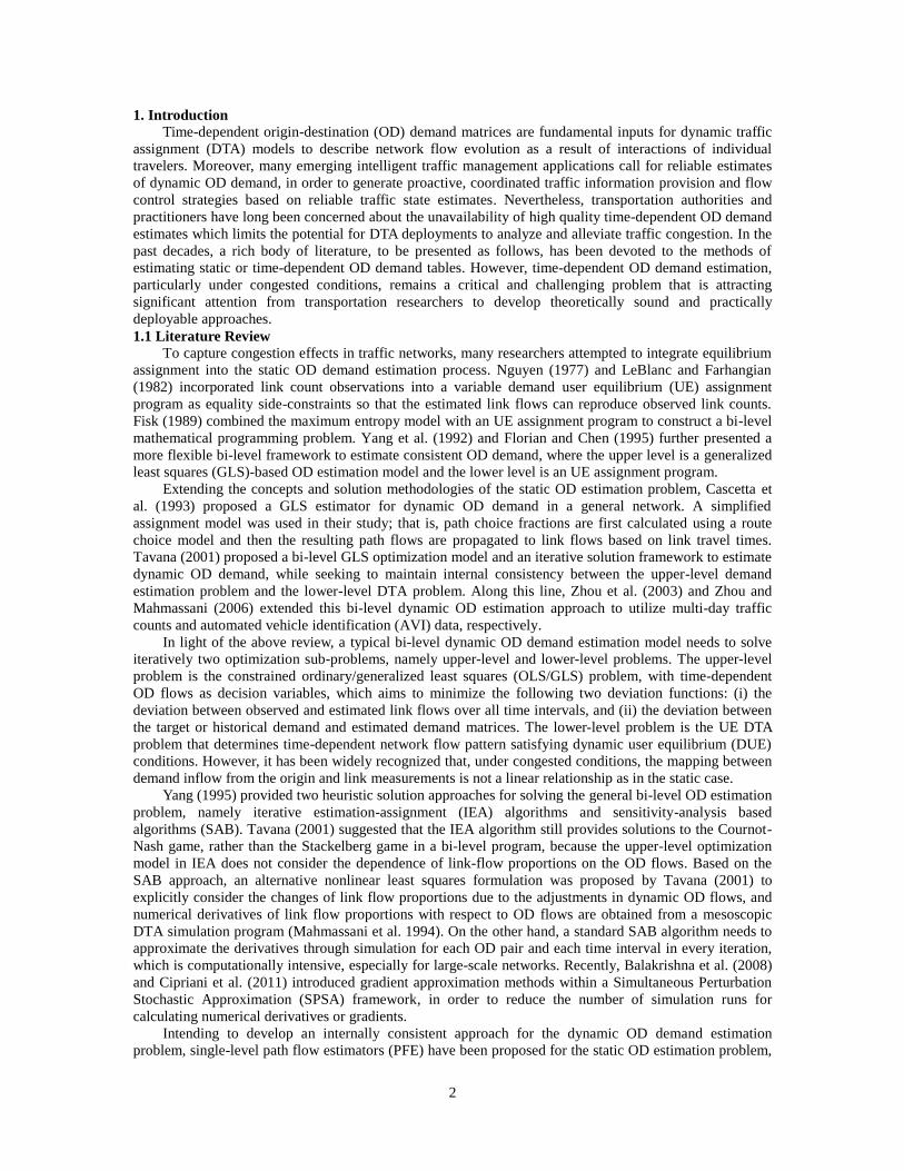
For instance, Fig. 14 shows the flow-density relationship for sensor b with jam density Kjam=120

vhc/ml/lane, free-flow speed Vf = 76 mph, backward wave speed w = 20 mph, and a maximum capacity of

1900 vhc/hour/lane.

(Boundary outflow capacity) One of the critical boundary conditions in this OD estimation problem is the

time-dependent maximum outflow discharge rate (i.e. capacity) on the downstream sensor d, which is a

result of the queue spillback from links further downstream and cannot be captured internally in the study

network. Thus, we use the historical average flow data to construct the link outflow capacity on station d

and set it as the fixed input for the DNL model.

(Historical demand) Based on the historical flow counts on the boundary sensors, namely, the stations on

freeway location a and all on-ramps, we estimate the total origin volume and then apply an estimated

destination split to setup a historical OD demand table, where the destination split assigns the majority of

flow toward the freeway destination d. This historical demand table serves as the target demand table in the

experiment.

(Initial demand table) To evaluate if and how the gradient-based algorithm can adjust a biased, initial OD

demand table toward the target demand table, we start with an OD demand table with only 70% of

historical demand volume.

Fig. 13 shows the observed time series of the traffic speeds at stations b, c and d. After 6:30 AM, the

traffic congestion from downstream location d is propagated to upstream sensors b and c, leading to a slow-

moving queue on freeway mainline segments between 7:00AM and 9:00AM. The traffic congestion starts

to dissipate afterwards, but the overall speed is still significantly below the free-flow level. The observed

flow pattern at entrance station a can be viewed as the total origin demand flow from station a to different

destinations. Error! Reference source not found. shows the estimated and observed flow patterns on

entry link a, and the corresponding average relative estimation errors are less than 10%. This indicates that

the proposed flow estimation algorithm can adjust a biased, initial demand pattern to match the target

demand volume at the entry point. The estimated space speeds and the observed point speeds at station c

are plotted in Fig. 15, which demonstrates that the DNL model is able to accurately reproduce the queue

spillback phenomenon along the corridor.

25

Fig. 13 Observed speed time series on freeway stations (demonstrating a congested period from 7:00AM to

9:00AM)

Fig. 14 Observed lane volume on station a vs. estimated lane volume on entrance link

0

10

20

30

40

50

60

70

80

90

6:00 AM 7:00 AM 8:00 AM 9:00 AM 10:00 AM

Sp

eed

(m

ph

)

Time

D

C

B

0

200

400

600

800

1000

1200

1400

1600

1800

2000

6:00 AM 7:00 AM 8:00 AM 9:00 AM 10:00 AM

La

ne

vo

lum

e (v

hc/

ho

ur)

Time

Observed lane volume

Estimated lane volume

0

10

20

30

40

50

60

70

6:00 AM 7:00 AM 8:00 AM 9:00 AM 10:00 AM

Sp

eed

(m

ph

)

Time

Observed speed

Estimated speed

26

Fig. 15 Observed point mean speed at station c vs. estimated space mean speed on the link from off-ramp h

to station c

5.3 Preliminary experiments on a real-world transportation network

The third set of numerical experiments is performed on a real-world subarea network within the

Portland, Oregon metropolitan area, which includes 858 nodes, 2000 links, and 208 origin-destination

zones shown. We first load a subarea OD demand matrix generated from a recent study (Kittelson et al.

2011) as the “true” OD demand, and use a DTA simulation program (based on Newell’s simplified KW

theory) to generate link density measures on 148 freeway links as the “ground-truth” observations in the

synthetic data set. The “true” OD demand leads to considerable traffic congestion in the network,

corresponding to an average trip speed of 23.15 mph. To assess the estimation performance of the proposed

approach, we define the mean absolute error (MAE) as

, (56)

where x(i) and y(i) are estimated and observed density, respectively. M is the number of samples. To

construct a slightly biased starting OD demand matrix, we apply a uniformly distributed random ratio

between [0.8, 1.0] to the ground-truth demand volume of each OD pair.

Fig. 16 MAE of the estimated link density as a function of iteration

Fig. 18 shows a decreasing pattern of the estimation error as the iterative algorithm proceeds. The final

MAE density value is about 15 vhc/mile/lane under congested conditions, which demonstrates that the

proposed algorithm is also able to produce accurate estimation results for this medium-scale network.

6. Concluding Remarks

With the particular focus on providing a consistent and efficient time-dependent path flow estimator,

this study proposes a new single-level, time-dependent OD demand estimation formulation, without using

link proportions, based on the mathematical program with complementary (DUE) constraints approach.

The proposed model is further reformulated as a gap-function-based nonlinear program. A Lagrangian

relaxation solution framework is developed to solve the proposed model. In each iteration, the tightest

upper bound is updated according to the DUE assignment results of the OD demand table constructed from

the estimated path flows, while the tightest lower bound is determined by the (gradient-projection-based)

path flow adjustment process. The algorithm proceeds until the gap between the upper bound and the lower

bound is minimized.

The mesoscopic DNL model, based on Newell’s simplified KW theory, is proposed to realistically

estimate network (link and path) performances for an estimated OD demand table. Furthermore, based on

0

5

10

15

20

25

30

0 5 10 15 20

Lin

k D

ensi

ty E

stim

ati

on

Err

or

(veh

icle

s/m

iles

/la

ne)

Iterations of Path Flow Adjustment

27

the DNL model, we derive theoretically sound partial derivatives of link flow, density and travel time with

respect to path flow perturbations, which are essential to determine the feasible descent direction in the

gradient-projection-based algorithm. The proposed OD demand flow estimation model and algorithm

utilize a wide variety of traffic measurements available from traffic sensor networks, and circumvent the

difficulty of providing complex mapping matrices between OD demand flows and those measurements in

most of the existing dynamic OD demand estimation methods. The seamless integration between the path

flow estimation and DTA models provides an effective and efficient way of utilizing heterogeneous data

sources. The application to the three test networks demonstrates the effectiveness and performance of the

proposed models under different network and data availability conditions.

In addition to examining its performance on large-scale networks in our future studies, the presented

joint assignment and flow estimation model has considerable potential for generalizing the modeling

framework into the field of real-time traffic state estimation and prediction. This would require further

investigation into numerous issues, such as calibrating the maximum queue discharge rates which critically

affect flows on downstream links, utilizing emerging end-to-end AVI travel times collected from Bluetooth

readers, and accommodating possible modeling errors and behavioral heterogeneity in the DUE

assignment.

Acknowledgement

The authors appreciate Professor Hani S. Mahmassani’s instructions and guidance for the fundamental

knowledge of dynamic traffic assignment. We would also like to thank Mr. Jeffrey Taylor for his valuable

suggestions. The work presented in this paper remains the sole responsibility of the authors.

References

Aashtiani, H. Z., Magnanti, T. L., 1981. Equilibria on a Congested Transportation Network. SIAM. Journal

on Algebraic and Discrete Methods 2(3), 213-226

Balakrishna, R., Ben-Akiva, M., Koutsopoulos, H. N., 2008. Time-dependent origin-destination estimation

without assignment matrices, in Transport Simulation: Beyond Traditional Approaches, Chung, E. and

Dumont, A.-G. (eds), EPFL Press, 201-213.

Bazara’a, M., Sherali, H., Shetty, C., 1993. Nonlinear Programming: Theory and Algorithms, second

edition. John Wiley & Sons, NY, USA.

Beckmann, M., McGuire, C. B., Winsten, C. B., 1956. Studies in the economics of transportation. Yale

University Press, New Haven, CT, USA.

Bell, M., Shield, C., Busch, F. and Kruse, G., 1997. A stochastic user equilibrium path flow estimator,

Transportation Research Part C 5(3/4), 197–210.

Bertsekas, D. P., 1995. Nonlinear Programming. Athena Scientific, Belmont, MA, USA.

Carey, M., 1987. Optimal time-varying flows on congested networks. Operations Research 35(1), 56-69.

Cascetta, E., Inaudi, D. and Marquis, G., 1993. Dynamic estimators of origin-destination matrices using

traffic counts. Transportation Science 27(4), 363-373.

Cipriani, E., Florian, M., Mahut, M., Nigro, M., 2011. A gradient approximation approach for adjusting

temporal origin–destination matrices. Transportation Research C 19(2), 270-282.

Daganzo, C.F., 1994. The cell transmission model: A dynamic representation of highway traffic consistent

with the hydrodynamic theory, Transportation Research Part B 28(4), 269-287.

Fisk, C. S., 1989. Trip matrix estimation from link traffic counts: the congested network case.

Transportation Research Part B 23(5), 331-336.

Florian, M., & Chen, Y., 1995. A coordinate descent method for the bi-level o-d matrix adjustment problem.

International Transactions in Operational Research 2(2), 165–179.

Friesz, T.L., Luque, J., Tobin, R.L., Wie, B.-W., 1989. Dynamic network traffic assignment considered as a

continuous time optimal control problem. Operations Research 37(6), 893-901.

Ghali, M.O. and Smith, M.J., 1995. A model for the dynamic system optimum traffic assignment problem.

Transportation Research Part B 29(3), 155-170.

Hurdle, V. F., Son, B., 2000. Road test of a freeway model. Transportation Research Part A 34(7), 537-564.

Kittelson, W., Rouphail, N., Williams, B. Zhou, X. 2011. Analyzing Operational Improvements as an

Alternative to Traditional Highway Construction, Transportation Research Board of the National

Academies CD-ROM, Paper #11-0714, presented at the 90th Annual Meeting of Transportation

Research Board, Washington D. C., USA.

Lawphongpanich, S., Hearn, D., 2004. An MPEC Approach to Second Best Toll Pricing. Mathematical

28

Programming 101(1), 33-55.

Leblanc, L.J. and Farhangian, K., 1982. Selection of a Trip Table which Reproduces Observed Link Flows.

Transportation Research Part B 16(2), 83-88.

Levinson, D. M., 2002. Road pricing and compensation for delay. Transportation Research Board of the

National Academies CD-ROM, Paper #02-2017, presented at the 81th

Annual Meeting of Transportation

Research Board, Washington D. C., USA.

Lighthill, M.J., Whitham, G.B., 1955. On kinetic wave II: a theory of traffic flow on crowded roads.

Proceedings of the Royal Society of London, Series A 229(1178), 317- 345.

Lo, H. K. and Chen, A., 2000. Reformulating the general traffic equilibrium problem via a smooth gap

function. Mathematical and Computer Modeling 31(2/3), 179-195.

Lu, C.-C., Mahmassani, H. S., Zhou, X., 2009. Equivalent gap function-based reformulation and solution

algorithm for the dynamic user equilibrium problem. Transportation Research Part B 43(3), 345-364

Mahmassani, H. S., Hu, T-Y, Peeta, S., and Ziliaskopoulos, A., 1994. Development and testing of dynamic

traffic assignment and simulation procedures for ATIS/ATMS applications. Report DTFH61-90-R-

00074-FG, U.S. DOT, Federal Highway Administration, McLean, VA, USA.

Merchant, D. and Nemhauser, G., 1978. A model and an algorithm for the dynamic traffic assignment

problem. Transportation Science 12(3), 183-199.

Newell, G. F., 1993. A simplified theory on kinematic waves in highway traffic, part I: general theory.

Transportation Research Part B 27(4), pp. 281-287.

Nguyen, S., 1977. Estimating an OD matrix from network data: A network equilibrium approach,

Publication No. 87, Centre de Recherche sur les Tranports, Universite de Montreal, Montreal, Quebec.

Nie, Y, Zhang, H. M., Recker, W. W., 2005.Inferring origin-destination trip matrices with a decoupled

GLS path flow estimator. Transportation Research Part B 39(6), 497–518

Nie, Y. and Zhang, H.M., 2008. A variational inequality approach for inferring dynamic origin-destination

travel demands. Transportation Research Part B 42(7), 635-662.

Nie, Y. and Zhang, H.M., 2010. A relaxation approach for estimating origin-destination trip tables.

Networks and Spatial Economics 10(1), 147-17

Qian, Z. and Zhang, H.M., 2011. Computing individual path marginal cost in networks with queue

spillbacks. Forthcoming in Transportation Research Record.

Richards, P.I., 1956. Shock waves on the highway. Operations Research 4(1), 42-51.

Scholtes, S. 2001. Convergence properties of a regularization scheme for mathematical programs with

complementarity constraints. SIAM Journal on Optimization 11, 918–936.

Shen, W., Nie, Y., Zhang, H. M., 2007. On path marginal cost analysis and its relation to dynamic system-

optimal traffic assignment. In: Allsop, R.E., Bell, M.G.H., and Heydecker, B.G. (Eds), Transportation

and Traffic Theory, Elsevier, 319-352.

Shen, W., and Wynter, L., 2011. A new one-level convex optimization approach for estimating origin-

destination demand. IBM Research Report, RC25147.

Sherali, H.D., and Park, T., 2001. Estimation of dynamic origin-destination trip tables for a general network.

Transportation Research Part B 35(3), 217-235.

Smith, M. J., 1993. A new dynamic traffic model and the existence and calculation of dynamic user

equilibrium on congested capacity-constrained road networks. Transportation Research Part B27(1), 49-

63.

Tavana, H., 2001. Internally-consistent estimation of dynamic network origin-destination flows from

intelligent transportation systems data using bilevel optimization. Ph.D. Dissertation, The University of

Texas at Austin.

Varaiya, P., 2002. California's performance measurement system: improving freeway efficiency through

transportation intelligence. TR News 218, 18-24.

Yang, H., Sasaki, T., Iida, Y. and Asakura, Y., 1992. Estimation of origin-destination matrices from link

traffic counts on congested networks. Transportation Research Part B 26(6), 417-434.

Yang, H., 1995. Heuristic algorithms for the bilevel origin-destination matrix estimation problem.

Transportation Research Part B 29(4), 231-242.

Zhou, X., Qin, X. and Mahmassani, H. S., 2003. Dynamic origin-destination demand estimation using

multi-day link traffic counts for planning applications. Transportation Research Record1831, 30-38.

Zhou, X. and Mahmassani. H. S., 2006. Dynamic OD demand estimation using automatic vehicle

identification data. IEEE Transactions on Intelligent Transportation Systems 7(1), 105- 114.

Ziliaskopoulos, A. K., Mahmassani, H. S., 1993. Time dependent shortest-path algorithm for real-time

29

Intelligent Vehicle Highway System applications. Transportation Research Record 1408, 94-100.