dynamic prediction of disease progression for leukemia

The Annals of Applied Statistics2017, Vol. 11, No. 3, 1649–1670DOI: 10.1214/17-AOAS1050© Institute of Mathematical Statistics, 2017

DYNAMIC PREDICTION OF DISEASE PROGRESSION FORLEUKEMIA PATIENTS BY FUNCTIONAL PRINCIPAL

COMPONENT ANALYSIS OF LONGITUDINALEXPRESSION LEVELS OF AN ONCOGENE

BY FANGRONG YAN∗,†,1, XIAO LIN∗ AND XUELIN HUANG†,2

China Pharmaceutical University∗ and The University of TexasMD Anderson Cancer Center†

Patients’ biomarker data are repeatedly measured over time during theirfollow-up visits. Statistical models are needed to predict disease progressionon the basis of these longitudinal biomarker data. Such predictions must beconducted on a real-time basis so that at any time a new biomarker mea-surement is obtained, the prediction can be updated immediately to reflectthe patient’s latest prognosis and further treatment can be initiated as nec-essary. This is called dynamic prediction. The challenge is that longitudinalbiomarker values fluctuate over time, and their changing patterns vary greatlyacross patients. In this article, we apply functional principal components anal-ysis (FPCA) to longitudinal biomarker data to extract their features, and usethese features as covariates in a Cox proportional hazards model to conductdynamic predictions. Our flexible approach comprehensively characterizesthe trajectory patterns of the longitudinal biomarker data. Simulation stud-ies demonstrate its robust performance for dynamic prediction under variousscenarios. The proposed method is applied to dynamically predict the riskof disease progression for patients with chronic myeloid leukemia followingtheir treatments with tyrosine kinase inhibitors. The FPCA method is appliedto their longitudinal measurements of BCR-ABL gene expression levels dur-ing follow-up visits to obtain the changing patterns over time as predictors.

1. Introduction. Precision medicine has been cast as the future of medicalcare, which has increased interest in prognostic models for many diseases. Ex-amples of such models available in the literature include prognostic models forvarious types of cancer, such as liver cancer, prostate cancer, and leukemia. How-ever, the majority of prognostic models in the literature provide risk predictionsusing only a small portion of the recorded information. Patient outcomes are typ-ically measured repeatedly over time, yet only the last one or two measurementsare used in prognostic models. An advantage of such a simple model is that it can

Received January 2016; revised April 2017.1Supported by the National Social Science Fund of China (No. 16BTJ021).2Supported by the US National Science Foundation Grant DMS-1612965, National Institutes of

Health Grants U54 CA096300, U01 CA152958, and 5P50 CA100632.Key words and phrases. Dynamic prediction, functional principal component analysis, longitudi-

nal biomarker, joint modeling, survival analysis.

1649

http://www.imstat.org/aoas/

http://dx.doi.org/10.1214/17-AOAS1050

http://www.imstat.org

1650 F. YAN, X. LIN AND X. HUANG

be easily applied in everyday clinical practice. However, an important limitation isthat valuable information is discarded, which, if appropriately used, could offer abetter insight into the dynamics of disease progression. In particular, an inherentcharacteristic of many medical conditions is their dynamic nature. That is, diseaseseverity and the rate of disease progression not only differ from patient to patientbut also dynamically change over time for the same patient. It is critical to capturethese changing patterns and use this information to predict patients’ prognoses andmake medical decisions in a real-time fashion. Well-designed statistical methodsand software are needed for such dynamic predictions.

To construct real-time prediction models for time to next failure event usinglongitudinal biomarker data, while the current biomarker value is usually an im-portant predictor, quite often the changing pattern of biomarker values over timecontains more information and thus has higher predictive power. For example,the transcript level of the gene BCR-ABL is a good indicator of residual diseasefor chronic myeloid leukemia (CML) patients [Quintas-Cardama et al. (2014)].Figure 1 shows that three patients have similar BCR-ABL transcript levels at 20months, but their changing patterns before that are quite different. The patientwho has always maintained a decreasing pattern may have the best future outcome(longer time to disease progression). The other patient whose BCR-ABL valuesdecreased initially but had an increase after 10 months may experience diseaseprogression soon (worst outcome). The remaining patient has an almost constantBCR-ABL value over time. His/her outcome might be intermediate between theabove two scenarios. From these hypothetical examples, we can see that it is im-portant to incorporate biomarker changing patterns into prediction models.

FIG. 1. Three hypothetical examples of changing patterns of BCR-ABL transcript levels over time:always decreasing, flat, decreasing first, and then bounce back. These patterns may indicate verydifferent future prognosis, despite similar BCR-ABL levels at the 20th month.

DYNAMIC PREDICTION 1651

The traditional survival analysis literature has provided many models for esti-mating the time to an event of interest. However, many of them incorporate base-line covariates only [Zheng, Cai and Feng (2006), Uno et al. (2007)], which meansthat such models can only be used to predict survival at the baseline. Recent workhas focused on the dynamic prediction of future survival at any time point be-yond the baseline [Huang et al. (2016)]. For this purpose, jointly modeling longi-tudinal information and survival data has been broadly used. The joint modellingapproach usually uses a parametric trajectory model with random effects for lon-gitudinal data, which are used as time-dependent covariates in a Cox proportionalhazards model [Wulfsohn and Tsiatis (1997), Tsiatis and Davidian (2001), Xu andZeger (2001), Song, Davidian and Tsiatis (2002), Ibrahim, Chen and Sinha (2004),Huang and Liu (2007), Liu and Huang (2009), Rizopoulos (2011), Rizopoulos andGhosh (2011), Rizopoulos et al. (2014)]. However, the nature of the longitudi-nal biomarker trajectory differs in each specific clinical setting. Therefore, it isdifficult to identify a satisfactory parametric family to use in modeling longitudi-nal biomarker data in all situations. Based on this consideration, others have usedsegmented mixed effect models [Slate and Turnbull (2000)], change point models[Pauler and Finkelstein (2002)], and B-splines [Brown, Ibrahim and DeGruttola(2005)] to characterize longitudinal biomarker trajectories.

Although many nonparametric methods, such as splines and kernel smoothing,have been applied to models for longitudinal biomarkers, they aim to better fit thebiomarker trajectories over time, and then use the fitted (denoised) biomarker val-ues to do prediction. In this article, while we can keep these denoised biomarkervalues as predictors, we also use a functional principal component analysis (FPCA)approach to extract the changing patters (features) of each individual’s biomarkertrajectory, and then use these features as additional predictors to improve the pre-diction. The FPCA is employed to characterize the pattern of random trajectoriesof repeatedly measured biomarkers [Besse and Ramsay (1986), Rice and Silver-man (1991), Silverman (1996), James, Hastie and Sugar (2000), Yao et al. (2003),Yao, Müller and Wang (2005), Yao and Lee (2006), Hall, Müller and Wang (2006),Liu and Yang (2009), Berkey and Kent (2009)]. It attempts to identify the dominantmodes of variation in a sample of trajectories around an overall mean trend func-tion. Under this framework, we construct our dynamic prediction models in twosteps. We first decompose different patterns of biomarker changes over time, andthen use the feature information extracted from this decomposition to make predic-tions. Simulation studies in Section 4 show that our proposed method has robustperformance, reflected by a larger area under the curve (AUC) of receiver’s operat-ing characteristics (ROC), and smaller residual mean square errors (RMSE), whencomparing some joint models with misspecified biomarker submodels. When com-paring correctly specified joint models, our AUCs and RMSEs are close to them.

The rest of this article is organized as follows. In Section 2, we introduce achronic myeloid leukemia (CML) dataset that motivated this research. In Sec-tion 3, we briefly review FPCA for longitudinal biomarkers measured at irregu-lar time intervals and obtain FPCA scores to characterize the trajectory pattern of


data observed during the entire span of patient follow-up time. Then, we providethe dynamic prediction based on the FPCA scores. In Section 4, we introduce theformulations of joint modeling and describe simulations we performed to compareour proposed method with some commonly used joint modeling approaches. Weillustrate the application of our technique to the CML dataset in Section 5, andprovide concluding remarks in Section 6.

2. A motivating example. This article is motivated by a study of CML thatfocused on the early detection of disease progression [Quintas-Cardama et al.(2014)]. Up to 95% of patients diagnosed with CML have a BCR-ABL fusion gene.Fusion genes result from the abnormal joining of DNA from two genes (genes BCRand ABL in this example) as a result of inversion or translocation. Tyrosine kinaseinhibitors (TKIs) have been used since year 2000 to stop the expression of BCR-ABL in CML patients. After treatment with TKIs, a large fraction of patients willachieve some level of good response, defined by improved clinical symptoms andreduced BCR-ABL expression levels. These patients then take the TKI drugs dailyfor life (until they become resistant to the drug), and have regular follow-up visits.Residual evidence of CML can be represented by the transcript level of BCR-ABL.The best outcome for patients is to achieve major molecular response (MMR),which is defined as the BCR-ABL transcript level standardized by the internationalscale as less than 0.1%. This value is simply denoted as 0.1, and similarly donethereafter in this article for all the BCR-ABL values (i.e., the % sign is removed).Some patients may never achieve MMR, but they are still free of clinical symp-toms of CML, and do not need any additional treatments. Their disease may re-main under control for many years with an almost constant low level of BCR-ABLexpression. However, CML may progress with increased levels of BCR-ABL. Thecommon clinical practice has been to wait until patients show symptoms of diseaseprogression to start new treatments. However, for many patients, their BCR-ABLtranscript levels increase before clinical symptoms of disease progression appear.Thus, it will be helpful to use this biomarker to predict the time to disease progres-sion so that physicians can initiate new treatments early to prevent it.

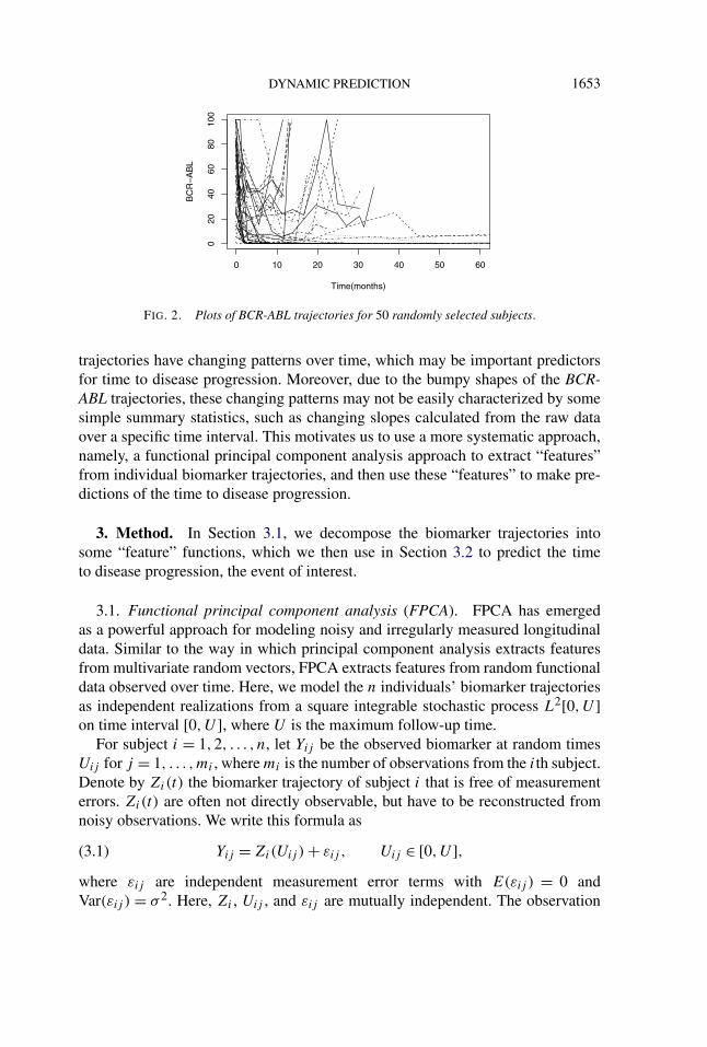
Imatinib and dasatnib are first and second-generation TKIs. The study underconsideration was a randomized trial that used second-line TKI therapy to treat670 patients with CML in a dose optimization phase and compared different doseschedules of dasatinib in patients with chronic phase CML, who had become re-sistant to imatinib therapy. A 6-year update of this study showed similar efficacyresults across the 4 dose schedules tested. In this article, we do not consider thecomparison between the 4 dose schedules, but focus on the dynamic predictionof disease progression using longitudinal BCR-ABL transcript levels. All patientswere followed every 3 months in the first year, every 6 months in the second year,and annually thereafter. The transcript levels of BCR-ABL were measured by apolymerase chain reaction during these follow-up visits. For illustration purposes,Figure 2 shows the BCR-ABL trajectories for 50 randomly selected patients. These


FIG. 2. Plots of BCR-ABL trajectories for 50 randomly selected subjects.

trajectories have changing patterns over time, which may be important predictorsfor time to disease progression. Moreover, due to the bumpy shapes of the BCR-ABL trajectories, these changing patterns may not be easily characterized by somesimple summary statistics, such as changing slopes calculated from the raw dataover a specific time interval. This motivates us to use a more systematic approach,namely, a functional principal component analysis approach to extract “features”from individual biomarker trajectories, and then use these “features” to make pre-dictions of the time to disease progression.

3. Method. In Section 3.1, we decompose the biomarker trajectories intosome “feature” functions, which we then use in Section 3.2 to predict the timeto disease progression, the event of interest.

3.1. Functional principal component analysis (FPCA). FPCA has emergedas a powerful approach for modeling noisy and irregularly measured longitudinaldata. Similar to the way in which principal component analysis extracts featuresfrom multivariate random vectors, FPCA extracts features from random functionaldata observed over time. Here, we model the n individuals’ biomarker trajectoriesas independent realizations from a square integrable stochastic process L2[0,U ]on time interval [0,U ], where U is the maximum follow-up time.

For subject i = 1,2, . . . , n, let Yij be the observed biomarker at random timesUij for j = 1, . . . ,mi , where mi is the number of observations from the ith subject.Denote by Zi(t) the biomarker trajectory of subject i that is free of measurementerrors. Zi(t) are often not directly observable, but have to be reconstructed fromnoisy observations. We write this formula as

(3.1) Yij = Zi(Uij ) + εij , Uij ∈ [0,U ],where εij are independent measurement error terms with E(εij ) = 0 andVar(εij ) = σ 2. Here, Zi , Uij , and εij are mutually independent. The observation


time points Uij can be either the same across individuals (regular time intervals)or differently and irregularly spaced for each individual.

Let Zi(t), i = 1, . . . , n be n independent realizations of the same square-integrable stochastic process Z(t), which has the mean function E[Zi(u)|Ti ≥u] = μ(u) and covariance function E[{Zi(u) − μ(u)} × {Zi(v) − μ(v)}|Ti ≥u, v] = G(u,v), for u, v ∈ [0,U ], where Ti is the survival time for subject i. Here,G(u,v) is symmetric about u and v, nonnegative definite. According to Mercer’stheorem [Leng and Müller (2006)], there exists a square integrable orthonormalbasis {ρk(u),0 ≤ u ≤ U,k = 1, . . . ,∞} (eigenfunctions) and {λk, k = 1, . . . ,∞}(eigenvalues) such that

(3.2) G(u,v) =∞∑

k=1

λkρk(u)ρk(v),

where ρk(v) is the orthonormal eigenfunction in L2[0,U ] corresponding to theeigenvalue λk for λ1 ≥ λ2 ≥ · · · > 0. This decomposition provides a basic toolto describe the distribution of the random trajectories Zi . We use the Karhunen-Loeve decomposition [Yao, Müller and Wang (2005)], which represents the meanof a random curve Zi(t) (biomarker trajectory for subject i), as

(3.3) Zi(u) = μ(u) +∞∑

k=1

γikρk(u), i = 1, . . . , n,

where γik = ∫ U0 {Zi(t) − μ(t)}ρk(t) dt is the kth FPCA score of random trajec-

tory Zi(t), 0 ≤ t ≤ U . Since ρk(t) and ρj (t), 0 ≤ t ≤ U are orthogonal for j �= k,the random variables γik , 1 ≤ k < ∞ are not correlated with each other, whileE(γik) = 0 and Var(γik) = λk . A good approximation of the equation (3.3) usuallycan be achieved by using only the first few components of the above decomposi-tion. That is to say,

(3.4) Zi(u) ≈ μ(u) +K∑

k=1

γikρk(u), i = 1, . . . , n.

The choice of K can be based on the fraction of variance as explained by Yao,Müller and Wang (2005) or some information criterion, which we introduce later.

The value of γik measures the similarity between Zi(t) − μ(t), the deviation ofindividual curve Zi(t) from the population mean, and the kth eigenfunction ρk(u).The above FPCA framework for functional data is a flexible method for capturingthe trajectories of longitudinal biomarker data. It is analogous to the representationof random vectors in multivariate analysis by principal components, in which arandom vector can be represented as a linear combination of the orthonormal basisdefined by the eigenvectors of its covariance matrix.

We use the principal analysis by conditional estimation (PACE) algorithm [Yao,Müller and Wang (2005)] to estimate the mean function μ(u), covariance function


G(u,v), eigenfunction ρk(t), and FPCA scores γik from the entire set of observeddata {Yij , i = 1, . . . , n, j = 1, . . . ,mi}. The PACE method has been shown to beversatile and powerful when applied to sparse and irregularly measured longitu-dinal data contaminated with measurement errors. Briefly, the PACE method car-ries out FPCA as follows using the data {(Uij , Yij ), i = 1, . . . , n, j = 1, . . . ,mi}.First, we estimate μ(u) of the mean function μ(u), which is obtained by a one-dimensional kernel smoother, such as a local linear smoother. Second, the estimatecovariance G(u, v), given u, v ∈ [0,U ], is obtained by a two-dimensional kernelsmoother with all pairwise products {Yij − μ(tij )}{Yil − μ(til)} for j �= l as theresponse and (tij , til) as the predictors. Details about how smoothing parameterswere chosen can be found in Yao, Müller and Wang (2005) and Dai et al. (2016).The smoothing techniques in these two steps are conducted over all the subjectswho are still at-risk at time u. Third, the estimates of eigenfunctions and eigenval-ues correspond to the solution ρk , λk of the equation

(3.5)∫U

G(u, v)ρk(u) du = λkρk(v), k ≥ 1,

where the ρk are subject to∫U ρ2

k (u) du = 1 and∫U ρk(u)ρl(u) du = 0 for l �= k.

Based on the above results, we can estimate γik = ∫(Zi(t) − μ(t))ρk dt by in-

tegration. Yao, Müller and Wang (2005) provides an alternative method to avoidnumerical integration. Their PACE method takes measurement errors and sparsemeasurements into account by assuming γik and εij to be mutually indepen-dent and predicting the random effects γik based on its conditional expectation:γik = E(γik|Yi). Predictions for γik are then obtained by plugging in estimatesof the parameters from the entire dataset, borrowing information from all sub-jects. Specifically, let Yi = (Yi1, . . . , Yimi

)′, μi = (μ(ti1), . . . ,μ(timi))′, and ρik =

(ρk(ti1), . . . , ρk(timi))′. Write Zi = (Zi1, . . . ,Zimi

)′, then let �Yi= cov(Yi, Yi) =

cov(Zi,Zi) + σ 2Imi. That is to say, the (j, l) entry of the mi × mi matrix �Yi

is(�Yi

)j,l = G(tij , til) + σ 2δjl with δjl = 1 if j = l, and 0 otherwise. Note that thediagonal terms (j = l) have an σ 2 term. That is why the above G(u, v) in (3.5) wasobtained without including those terms {Yij − μ(tij )}{Yil − μ(til)} with j = l inthe computaion. On the other hand, applying local linear smoother to these termswith j = l, an estimator V (t) for G(t, t) + σ 2 is obtained. Consequently, σ 2 canbe estimated by

(3.6) σ 2 = 2

U

∫ 3U/4

U/4

{V (t) − G(t, t)

}dt,

where the interval [U4 , 3U

4 ] is used to mitigate boundary effects. Staniswalis andLee (1998) showed in their Theorem 2 that under certain regularity conditions, the


estimator for σ 2 is consistent. Following the above process, we can obtain

(3.7) γik = E(γik|Yi) = λkρ′ik�

−1Yi

(Yi − μi).

To choose K , which is the number of eigenfunctions needed to provide a rea-sonable approximation for the infinite-dimensional process, we may use the cross-validation score based on the leave-one-out prediction error [Rice and Silverman(1991)]. Let μ(−i) and ρ

(−i)k be the estimated mean and eigenfunctions after re-

moving the data for the ith subject. Then, we choose K so as to minimize thecross-validation score based on the squared prediction error,

(3.8) CV(K) =n∑

i=1

mi∑j=1

{Yij − Y

(−i)i (tij )

}2,

where Y(−i)i is the predicted curve for the ith subject, computed after removing the

data for this subject, that is, Y(−i)i (t) = μ(−i)(t) + ∑K

k=1 γikρ(−i)k (t), where γik is

estimated by (3.7).Alternatively, we may use an adapted Akaike information criterion (AIC).

A pseudo-Gaussian log-likelihood L can be defined as the sum of the contributionsfrom all subjects, treating the estimated FPCA scores γik as normally distributedwith variance σ 2 and independent across both i and k, as below,

(3.9) L =n∑

i=1

{−mi

2log

(2πσ 2) − 1

2σ 2

mi∑j=1

(Yij − ZK

i (tij ))2

}.

Then, let AIC = −L+K . It has been showed that this AIC is computationally moreefficient and achieves results that are similar to those obtained by cross-validation[Yao, Müller and Wang (2005)].

3.2. Survival analysis with longitudinal biomarker data. The FPCA scoresγik can be estimated from the observation {Yi1, . . . , Yi,mi

}. In this section, weshow how to use those FPCA scores in the survival analysis. Assume that theinfinite-dimensional covariate trajectories Zi(t) under consideration are well ap-proximated by the projection onto the function space spanned by K eigenfunc-tions. The estimated trajectory Zi(t) for the ith subject, using the first K eigen-functions, is given by

(3.10) ZKi (t) = μ(t) +

K∑k=1

γikρk(t), t ∈ [0,U ].

The number of eigenfunctions, K , can be chosen by cross-validation based onthe AIC or leave-one-out prediction error. Given the estimates μ(t) and ρk (k =1, . . . ,K), the various FPCA scores γik result in different trajectory patterns.Therefore, the FPCA scores γik can be used as covariates in modeling the rela-tionship between the survival time and the patterns of the trajectories.


Let Ti and Ci denote the event and censoring times, respectively, and assumeCi is independent of biomarker measurements. Rather than observe Ti for all i, weobserve only Vi = min(Ti,Ci) and i = I (Ti ≤ Ci). Let Xi be a q-dimensionalvector of the baseline covariates and let Zi(t), t ≥ 0, be the longitudinal biomarkertrajectory for subject i. Our consideration of the baseline covariates for simplicitydoes not alter the general insights we highlight in the next section. The followingapproach is commonly used for dynamic prediction. For subject i, assume a Coxproportional hazards model [Cox (1972)] that specifies hi(t), the hazard functionfor Ti as

(3.11) hi

(t |Xi,Zi(t)

) = h0(t) exp{θ ′Xi + αZi(t)

},

where h0(t) is an arbitrary non-negative function, and θ and α are unknown pa-rameters.

The above approach uses the biomarker values measured at time t only. It mayuse historical biomarker values in some ad hoc way, such as letting Z(t) be thebiomarker value change or changing rate from the previous observation. However,these approaches may not be sufficient to fully capture the longitudinal biomarkerinformation. In many situations, the biomarker trajectory features (changing pat-terns) are more important than the current biomarker value or recent changingmagnitude or slope, in terms of predicting a future event. In the decomposition,equation (3.3), each ρ(u), u ∈ [0,U ] may be viewed as a changing pattern, andγik describes how strongly the data from subject i follow this pattern. Our idea isto use γik , k = 1, . . . ,K , as predictors. With this preparation, we conduct dynamicprediction at any time t using the following model:

(3.12) hi(t |Xi, γi) = h0(t) exp{θ ′Xi + β ′γi

},

where β = (β1, . . . , βK)′ are the regression coefficients for the K estimated FPCAscore vector γi = (γi1, . . . , γiK)′, and θ = (θ1, . . . , θq)

′ are the regression coeffi-cients for the baseline covariates.

In the above, for simplicity, we use the Cox (1972) proportional hazards modelfor prediction. However, in practice, it is important to test whether the proportionalhazards assumption holds. A few different approaches have been proposed to testthis assumption. For a categorical covariate, we may plot the estimated cumulativehazard functions for different levels of this variable, and check whether they areparallel of each other. For both continuous and categorical covariates, we may addto the model their interactions with a function of time, such as log(t). If someof these interactions terms turn out to be statistically significant, the proportionalhazards assumption is violated. In this case, those significant interaction termscan be added to the model to improve its goodness-of-fit [Cox (1972)]. Lin, Weiand Ying (1993) proposed to check the Cox model assumption with cumulativesums of martingale-based residuals. Their method has been implemented in SASProc Phreg (SAS Institute Inc., Cary, NC, USA). Grambsch and Therneau (1994)


provided a diagnosis test based on weighted residuals, which can be done by thecox.zph function in R (https://www.r-project.org/). Other approaches include Lin,Zhang and Davidian (2006), Grant, Chen and May (2014), among others.

3.3. Dynamic individualized predictions. To apply the above dynamic pre-diction method to an existing dataset, we first obtain estimated FPCA scores(γi1, . . . , γiK) using the longitudinal biomarker data, and then estimate θ , β ,h0(t) using the baseline covariates, survival information, and FPCA scores.Then, for a new subject (not in the dataset) with baseline covariate Xn+1and biomarker measurements Yn+1 = (Yn+1,1, . . . , Yn+1,mn+1)

′ at time pointsUn+1,1, . . . ,Un+1,mn+1 ≤ U , we use the following formula to compute the FPCAscores for this subject:

(3.13)γn+1,k = E(γn+1,k|Yn+1)

= λkρ′n+1,k�

−1Yn+1

(Yn+1 − μn+1), k = 1, . . . ,K,

where ρ′n+1,k , �Yn+1 and μn+1 are computed similarly as done for ρ′

i,k , �Yiand μi ,

1 ≤ i ≤ n, in the preparation of equation (3.7). Then, the prediction for this newsubject can proceed as follows. At any time t after the last biomarker observation,that is, t ≥ Un+1,mn+1 , the predicted future survival distribution can be written as

(3.14)

Pr(Tn+1 ≥ t + u|Tn+1 > t,Xn+1, γn+1)

={S0(t + u)

S0(t)

}exp{θ ′Xn+1+β ′γn+1},

where S0(t) = exp{− ∫ t0 h0(u) du}, and S0(t) is its Breslow estimator [Breslow

(1972)] resulting from model (3.12). Note this prediction is dynamic, which meansit can be updated at any time, as soon as the subject n + 1 has new biomarkermeasurements. This is to simply replace the biomarker vector Yn+1 by its updatedversion, and then update equations (3.13) and (3.14) accordingly.

By using FPCA scores, we achieve the following advantages. First, a biomarkertrajectory model is not assumed, which is usually difficult to specify, and a mis-specified trajectory model may lead to biased predictions. Second, we obtain theFPCA scores using only the observed biomarker values. There is no need for allsubjects to have biomarker measurements made at the same post-baseline timepoint. Third, the proposed method can be used to continuously conduct and updatepredictive analyses over time.

4. Simulations. We conducted simulation studies under several scenarios tocompare our proposed method to joint modeling approaches with parametric mod-els for longitudinal biomarker trajectories, and assessed the advantages and disad-vantages of these approaches.

https://www.r-project.org/


4.1. Model specification. Most approaches for jointly modeling time-to-eventand longitudinal data are based on the Cox proportional hazards model with time-dependent covariates. Focusing on normally distributed longitudinal outcomes, weuse a linear mixed-effects model to generate the subject-specific longitudinal tra-jectories. Namely, we have

Yi(t) = Zi(t) + εi(t),

εi(t) ∼ N(0, σ 2)

,

where Zi(t) denotes the true (unobserved) value of the longitudinal biomarker datawithout error at time t , and Yi(t) is a measurement of Zi(t) with error εi(t). Then,we assume the hazard function of subject i is

(4.1) hi

(t |Zi(t)

) = h0(t) exp{αZi(t)

},

where h0(t) = λtλ−1 exp(η), a Weibull baseline hazard function with λ = 2,η = −5, and the association parameter α = 0.5. For the longitudinal process,we consider four different scenarios, including linear and nonlinear mixed-effectsmodels, to capture the variation of biomarkers for an individual subject, as follows.

I: Linear Model Zi(t) = a + bt + bi1 + bi2t,

II: Exponential Model Zi(t) = c exp(at) + bi1 + bi2t,

III: Quadratic Model Zi(t) = a(t − b)2 + c + bi1 + bi2t,

IV: Piecewise Function Model

Zi(t) =

⎧⎪⎪⎨⎪⎪⎩

Wi exp(−ait) + bi1 + bi2t, t ≤ 2,

di + bi1 + bi2t, 2 < t ≤ 5,

di + ci(t − 5)2 + bi1 + bi2t, t > 5.

In scenario I, a linear longitudinal trajectory is described with a = 1, b = −2. Inscenario II, an exponential trajectory is represented with a = 0.1, c = 3. Similarly,scenario III uses a quadratic model to generate a nonlinear longitudinal trajectorywith a = 0.2, b = 3, c = 1. Scenario IV defines a piecewise function trajectory,with Wi ∼ N(3,0.12), ai ∼ N(1,0.12), ci ∼ N(0.3,0.12), di ∼ N(0.3,0.12). Alltrajectories considered above use random effect terms bi = (bi1, bi2)

′ ∼ N(0,D),with D =

(0.4 0.10.1 0.2

). For simplicity, we generate longitudinal data on irregular time

points t = 0 and t = j + εij , j = 1,2, . . . ,10 and εij ∼ N(0,0.12) independentacross all i and j . Considering the existence of measurement error, we also setεi(t) ∼ N(0,0.62), independent of each other across i and t . We simulated thecensoring times from a uniform distribution in (0, tmax), with tmax set to result inabout 25% censoring in each scenario. Using the models and parameter settingsabove, we generated four scenarios of datasets. For each scenario, we simulated100 datasets with sample sizes n = 400.


The next step after generating the data for the four scenarios is to analyze thesedatasets with dynamic prediction methods. For each scenario, we considered fourdynamic prediction methods: our proposed method, FPCA, which uses a func-tional form to capture the variation of the longitudinal biomarker data, and threeapproaches that use a joint modeling framework: JML, JME and JMQ. JML usesa linear model as a fixed-effect term in a longitudinal data submodel; JME usesan exponential formula to model the main trend of the longitudinal data; and JMQemploys a quadratic expression to capture the non-monotonic longitudinal trajec-tories. The R package JM [Rizopoulos (2010)] was used to fit these joint models.

4.2. Measures to assess predictive performance. We use two measures to eval-uate the predictive performance of our proposed method. The first is the root meansquared errors (RMSEs) between the predicted survival probabilities and their truevalues (which are known in simulation studies). The second is the area under thereceiver’s operating characteristic curve (AUC). To compute AUC, we focus on atime interval of medical relevance (t, t + t). Let πi(t + t) represent the sur-vival probability for subject i at t + t . It has been proposed that the AUC can becomputed as follows [Harrell, Lee and Mark (1996), Heagerty and Zheng (2005),Antolini, Boracchi and Biganzoli (2005)]. For a randomly chosen pair of subjects{i, j} who have both provided measurements up to time t ,

(4.2)

AUC(t,t)

= Pr[πi(t + t |t) < πj (t + t |t)|{

T ∗i ∈ (t, t + t]} ∩ {

T ∗j > t + t

}].

That is, the AUC can be computed as a concordance measure between predictionsand observed events.

4.3. Analysis and results. In each scenario, we used all observations for 400subjects to fit the four dynamic predictive models (FPCA, JML, JME, and JMQ).The JML, JME and JMQ are the true models for scenarios I, II and III respec-tively. The FPCA approach used the FPCA scores obtained as in (3.7) as covari-ates to form the hazard function in equation (3.12). The FPCA scores represent thechanging patterns of the longitudinal observations throughout the time intervals.

We used the RMSE to assess calibration. The mean RMSEs and their standarddeviations over all subjects from the 100 datasets are shown in Table 1, for pre-dictions conducted at t = 4 for survival probability at t + t = 6. We used theAUC described above to similarly assess the discrimination ability of the four ap-proaches. For each simulated dataset and based on each joint model, we estimatedAUC(t = 2,t = 6) using all 400 subjects. The means and standard deviationsof AUCs from the 100 simulated datasets are shown in Table 2. From Tables 1and 2, we observe that for all scenarios, FPCA has robust predictive performance,in terms of both calibration and discrimination, outperforming joint models with


TABLE 1Simulation results: Mean (standard deviation) of the root mean squared prediction errors (RMSEs)by the four methods (JML, JME, JMQ, FPCA) in each scenario of longitudinal biomarker values as

a function of observation time (Linear, Exponential, Quadratic, Piecewise function models)

RMSE Linear Exponential Quadratic Piecewise

JML 0.09642 0.09831 0.15694 0.14949(0.00537) (0.01112) (0.00462) (0.01674)

JME 0.09698 0.09656 0.17599 0.15863(0.00537) (0.01100) (0.01819) (0.02641)

JMQ 0.09677 0.09840 0.15617 0.23850(0.00526) (0.01115) (0.01840) (0.06086)

FPCA 0.08537 0.07100 0.07218 0.08724(0.00785) (0.00948) (0.00938) (0.01975)

parametric biomarker models. The JM package had not implemented the computa-tion for conditional survival probabilities based on Cox proportional hazards mod-els with time-dependent covariates, so piecewise constant hazard functions wereassumed. This may have affected the performance of joint models for prediction.

FPCA is somewhat time-consuming compared to the other methods. Using apersonal computer (RAM 12 G, CPU 3.4 GHz) for the above simulation study, ittakes about 6 hours using FPCA, while it takes about 1 hour for each of JML, JMEand JMQ.

5. Application. We return to the CML dataset described in Section 2. Thiswas a study of 670 patients diagnosed with CML and enrolled in a trial to receive

TABLE 2Simulation results: Mean (standard deviation) of the area under the receiver’s operating

characteristics curve (AUCs) by the four methods (JML, JME, JMQ, FPCA) in each scenario oflongitudinal biomarker values as a function of observation time (Linear, Exponential, Quadratic,

Piecewise function models)

AUC Linear Exponential Quadratic Piecewise

JML 0.6634 0.7052 0.5057 0.5753(0.09681) (0.11995) (0.05239) (0.05877)

JME 0.6520 0.7070 0.5677 0.5783(0.09673) (0.11469) (0.05454) (0.05306)

JMQ 0.6542 0.6971 0.5712 0.5409(0.09874) (0.12827) (0.04857) (0.06424)

FPCA 0.6908 0.8613 0.6182 0.8487(0.09931) (0.07412) (0.05600) (0.04022)


FIG. 3. Kaplna–Meier estimator for time to disease progression.

dasatinib. Only 567 of the patients had BCR-ABL measurements taken both beforeand after the dasatinib treatment, and thus were included in our data analysis forthe prediction model. Figure 3 shows their progression-free survival distributionestimated by the Kaplan–Meier method [Kaplan and Meier (1958)] without usingthe information from their longitudinal BCR-ABL measurements. We are interestedin predicting progression-free survival probabilities for patients each time afterthey obtain their updated BCR-ABL measurements during follow-up visits.

Although patients are supposed to have follow-up visits at 3, 6, 9, 12, 18 and 24months, and every year thereafter, in reality, their visiting times are irregular dueto various constraints, and they may miss some of their scheduled visits. There-fore, patients and physicians would like to have updated predictions at any timeimmediately after new BCR-ABL measurements are available, rather than on justa few discrete time points. In order to handle irregular time intervals and sparseobservation data by the FPCA method introduced in Section 3, we decompose theBCR-ABL trajectories as

(5.1) Yij = μ(Uij ) +∞∑

k=1

γikρk(Uij ) + εij , Uij ∈ [0,U ].

The PACE method was employed to estimate the mean function μ(Uij ), eigen-value λk , and eigenfunction ρk(Uij ). With the resulting estimators μ(Uij ), λk ,ρk(Uij ) available, FPCA scores were obtained by equation (3.7). All calculationsmentioned above can be completed in R with the package “fpca.” The smoothedmean function of BCR-ABL is plotted in Figure 4. By adjusting grids in R functionfpca.mle(), we obtain smoother eigenfunctions and a mean function. The pattern of


FIG. 4. Mean function of BCR-ABL with functional principle component analysis.

the mean function demonstrates that most patients experience a sharp decrease atthe beginning of treatment (within about 15 months), followed by a slight decline.After 60 months, the mean BCR-ABL level increases substantially.

By applying the FPCA techniques, we obtain eigenfunctions, which are ba-sis functions to form biomarker trajectories, as defined in equations (3.2)–(3.4).The number of eigenfunctions was chosen using the cross-validation score. Threeeigenfunctions were chosen and shown in the bottom panels of Figure 5. Based onthe mean and eigenfunctions, the fitted biomarker trajectories for three randomlyselected subjects are shown in the top panels of Figure 5.

The FPCA scores represent the changing pattern of BCR-ABL levels over thewhole time interval. We used them to model the hazard function as below:

(5.2) hi(t) = h0(t) exp{β1γi1 + β2γi2 + β3γi3}.To check the proportional hazards assumption, the interaction terms γi1 log(t),

γi2 log(t), and γi3 log(t) are added to the model in (5.2). The parameter estima-tion of this extended model shows that γi3 and γi3 log(t) are not significant, withP-values 0.3984 and 0.3576, respectively, while the remaining four terms are allsignificant with P-values less than 0.01. This means the proportional hazards as-sumption is violated. So, we further improved model (5.2) by including two prin-cipal components γi1, γi2, and their interaction terms with log(t), as below:

(5.3) hi(t) = h0(t) exp{β1γi1 + β2γi2 + β3γi1 log(t) + β4γi2 log(t)

}.

Based on this model and equation (3.14), dynamic prediction can be performedto provide future survival rate estimation at time point t . In order to keep consistentwith simulation, here we also used FPCA, JML, JME, and JMQ to fit joint models.Figure 6 plots the estimated survival curves of a specific patient based on these


FIG. 5. Predicted trajectories with observed measurements (dots) and three eigenfunctions recov-ered by this method.

different prediction methods. It can be seen from this figure that the biomarkertrajectory of this patient shows a nonlinear decreasing trend, where linear, expo-nential, and quadratic longitudinal submodles may not be suitable to fit biomarkervalues. This may be the reason why JML, JME, and JMQ show similar suboptimalperformance. In contrast, FPCA uses a nonparametric method to extract dominantinformation from longitudinal biomarker, which may give more accurate predic-tion probabilities than the joint modeling approaches. Certainly these predictionsfor a particular subject are presented more for illustration, rather than the compar-ison of the performance between different methods.

The prediction performances of the aforementioned four methods are comparedbelow by their time-dependent AUC curves. That is, at a time point t , we conductprediction of disease-progression by time t + t , with t = 20 months. Then, wecompute the AUC of this prediction using the method defined in equation (4.2).


FIG. 6. Dynamic predictions for one patient by four models. Each panel shows the survival proba-bilities conditional on the longitudinal measurements up to the time point conducting the predictions.The predicted survival curves by “JML” and “JMQ” overlap.

This process is repeated for series of different time points t , and the results are plot-ted in Figure 7. We can see that our proposed FPCA method has the highest AUClevels over time, outperforming the joint models using linear (JML), quadratic(JMQ), and exponential (JME) submodels for longitudinal data. This may be ex-plained by the observation that, in this data set, the biomarkers do not follow alinear, quadratic, or exponential model. This can be reflected in the mean functionplot in Figure 4. On the other hand, the proposed FPCA method is flexible to fitbiomarker trajectories of all kinds of different shapes. This is a great advantage ofthe proposed method since the biomarker trajectories in the real world are alwaysmuch more complicated than the commonly used parametric forms.

For the Cox proportional hazards model in (5.2), we attempted to include somebaseline covariates such as patient age, race, and sex. However, these variables do


FIG. 7. Time-dependent AUC curves for dynamic predictions conducted at time t (the x-axis),for survival outcome at t + t , with t = 20 months: Comparison of prediction performance byfour methods of joint modelling longitudinal and survival data, with longitudinal data modelled byfunctional principal component analysis (FPCA, solid line), linear model (JML, dot line), quadraticmodel (JMQ, dash line) or exponential model (JME, dot–dash line)

not have much predictive power. Prediction at t = 40 months with t = 20 monthsby a Cox model with only these three variables results a low AUC value of 0.53.Adding the FPCA terms γ1, γ2, and γ3 improves the AUC to 0.62.

Yao, Müller and Wang (2005) imposed normal distribution assumptions for γik

and εik in deriving the FPC scores Histogram plots for γik and εij showing thatboth normal distribution assumption are satisfied (Figure 8).

In summary, accurate prediction of the risks of disease progression can helpphysicians and patients make better treatment decisions. For example, they maydecide that at any time when the risk of disease progression in the next year (orsix months) is greater than 20%, then they should start a prevention therapy. Ourproposed method can also help identify patients who are at elevated risks of diseaseprogression, and remind them to have more frequent follow-up visits.

6. Discussion. The relationship between longitudinal biomarker data andclinical outcomes is important in precision medicine. Conventional survival anal-ysis fits the Cox proportional hazards model, using biomarker data measured at aspecific time point as covariates. However, it is often the pattern of covariate valuesthat predicts a patient’s survival time. The aim of this article is to capture the tra-jectory pattern of longitudinal biomarker data within the collection period and use


FIG. 8. Histograms to check normality assumptions.

this summary information as predictors to conduct real-time dynamic predictionof the time to a specific event.

The simulation studies show that our proposed method can characterize the tra-jectory patterns of the covariates and have more robust performance than otherjoint modeling approaches that use parametric biomarker models. Our proposedmethod does not need to specify a model for the longitudinal biomarker, and thusavoids the bias caused by the misspecification of such a model. It performs wellunder various scenarios, demonstrating that it is a versatile and robust approachfor dynamic prediction.

A limitation of all principal component analysis approaches is that they are con-ducted independent of the outcomes, and thus the resulting order of the principalcomponents may not indicate the order of their predictive power. With this con-sideration, it warrants further research to explore alternative approaches, such asusing supervised functional principal component analysis for dynamic prediction.


We have assumed independence between censoring time and biomarker mea-surement. This assumption is reasonable for most types of administrative censor-ing, such as when censoring happen at the end of the study. If many subjects dropout of the study, then this assumption may not hold. To handle such a situation,we need to make changes to both the estimation of functional principal compo-nents and the survival modelling. It is important to consider such scenarios, whichwarrant further research.

REFERENCES

ANTOLINI, L., BORACCHI, P. and BIGANZOLI, E. (2005). A time-dependent discrimination indexfor survival data. Stat. Med. 24 3927–3944. MR2221976

BERKEY, C. and KENT, R. J. (2009). Longitudinal principal components and non-linear regressionmodels of early childhood growth. Ann. Hum. Biol. 10 523–536.

BESSE, P. and RAMSAY, J. O. (1986). Principal components analysis of sampled functions. Psy-chometrika 51 285–311. MR0848110

BRESLOW, N. E. (1972). Discussion of “Regression models and life-tables” by D. R. Cox. J. Roy.Statist. Soc. Ser. B 34 187–220.

BROWN, E. R., IBRAHIM, J. G. and DEGRUTTOLA, V. (2005). A flexible B-spline model for mul-tiple longitudinal biomarkers and survival. Biometrics 61 64–73. MR2129202

COX, D. R. (1972). Regression models and life-tables. J. Roy. Statist. Soc. Ser. B 34 187–220.MR0341758

DAI, X., HADJIPANTELIS, P. Z., JI, H., MUELLER, H. G. and WANG, J. L. (2016). Functional dataanalysis and empirical dynamics. Available at https://cran.r-project.org/web/packages/fdapace/fdapace.pdf.

GRAMBSCH, P. M. and THERNEAU, T. M. (1994). Proportional hazards tests and diagnostics basedon weighted residuals. Biometrika 81 515–526. MR1311094

GRANT, S., CHEN, Y. Q. and MAY, S. (2014). Performance of goodness-of-fit tests for the Coxproportional hazards model with time-varying covariates. Lifetime Data Anal. 20 355–368.MR3217542

HALL, P., MÜLLER, H.-G. and WANG, J.-L. (2006). Properties of principal component methodsfor functional and longitudinal data analysis. Ann. Statist. 34 1493–1517. MR2278365

HARRELL, F. E., LEE, K. L. and MARK, D. B. (1996). Multivariable prognostic models: Issuesin developing models, evaluating assumptions and adequacy, and measuring and reducing errors.Stat. Med. 15 361–387.

HEAGERTY, P. J. and ZHENG, Y. (2005). Survival model predictive accuracy and ROC curves.Biometrics 61 92–105. MR2135849

HUANG, X. and LIU, L. (2007). A joint frailty model for survival and gap times between recurrentevents. Biometrics 63 389–397. MR2370797

HUANG, X., YAN, F., NING, J., FENG, Z., CHOI, S. and CORTES, J. (2016). A two-stage approachfor dynamic prediction of time-to-event distributions. Stat. Med. 35 2167–2182. MR3513506

IBRAHIM, J. G., CHEN, M.-H. and SINHA, D. (2004). Bayesian methods for joint modeling oflongitudinal and survival data with applications to cancer vaccine trials. Statist. Sinica 14 863–883. MR2087976

JAMES, G. M., HASTIE, T. J. and SUGAR, C. A. (2000). Principal component models for sparsefunctional data. Biometrika 87 587–602. MR1789811

KAPLAN, E. L. and MEIER, P. (1958). Nonparametric estimation from incomplete observations.J. Amer. Statist. Assoc. 53 457–481. MR0093867

LENG, X. and MÜLLER, H.-G. (2006). Classification using functional data analysis for temporalgene expression data. Bioinformatics 22 68–76.

http://www.ams.org/mathscinet-getitem?mr=2221976




https://cran.r-project.org/web/packages/fdapace/fdapace.pdf










https://cran.r-project.org/web/packages/fdapace/fdapace.pdf


LIN, D. Y., WEI, L. J. and YING, Z. (1993). Checking the Cox model with cumulative sums ofmartingale-based residuals. Biometrika 80 557–572. MR1248021

LIN, J., ZHANG, D. and DAVIDIAN, M. (2006). Smoothing spline-based score tests for proportionalhazards models. Biometrics 62 803–812. MR2247209

LIU, L. and HUANG, X. (2009). Joint analysis of correlated repeated measures and recurrent eventsprocesses in the presence of death, with application to a study on acquired immune deficiencysyndrome. J. R. Stat. Soc. Ser. C. Appl. Stat. 58 65–81. MR2662234

LIU, X. and YANG, M. C. K. (2009). Identifying temporally differentially expressed genes throughfunctional principal components analysis. Biostatistics 10 667–679.

PAULER, D. and FINKELSTEIN, D. (2002). Predicting time to prostate cancer recurrence based onjoint models for non-linear longitudinal biomarkers and event time outcomes. Stat. Med. 21(24)3897–3911.

QUINTAS-CARDAMA, A., CHOI, S., KANTARJIAN, H., JABBOUR, E., HUANG, X. and CORTES, J.(2014). Predicting outcomes in patients with chronic myeloid leukemia at any time during tyro-sine kinase inhibitor therapy. Clin. Lymphoma Myeloma Leuk. 14 327–334.

RICE, J. A. and SILVERMAN, B. W. (1991). Estimating the mean and covariance structure nonpara-metrically when the data are curves. J. Roy. Statist. Soc. Ser. B 53 233–243. MR1094283

RIZOPOULOS, D. (2010). JM: An R package for the joint modelling of longitudinal and time-to-event data. J. Stat. Softw. 35 (9) 1–33.

RIZOPOULOS, D. (2011). Dynamic predictions and prospective accuracy in joint models for longi-tudinal and time-to-event data. Biometrics 67 819–829. MR2829256

RIZOPOULOS, D. and GHOSH, P. (2011). A Bayesian semiparametric multivariate joint model formultiple longitudinal outcomes and a time-to-event. Stat. Med. 30 1366–1380. MR2828959

RIZOPOULOS, D., HATFIELD, L. A., CARLIN, B. P. and TAKKENBERG, J. J. M. (2014). Combin-ing dynamic predictions from joint models for longitudinal and time-to-event data using Bayesianmodel averaging. J. Amer. Statist. Assoc. 109 1385–1397. MR3293598

SILVERMAN, B. W. (1996). Smoothed functional principal components analysis by choice of norm.Ann. Statist. 24 1–24. MR1389877

SLATE, E. and TURNBULL, B. (2000). Statistical models for longitudinal biomarkers of diseaseonset. Stat. Med. 19(4) 617–637.

SONG, X., DAVIDIAN, M. and TSIATIS, A. A. (2002). A semiparametric likelihood approach tojoint modeling of longitudinal and time-to-event data. Biometrics 58 742–753. MR1945011

STANISWALIS, J. G. and LEE, J. J. (1998). Nonparametric regression analysis of longitudinal data.J. Amer. Statist. Assoc. 93 1403–1418. MR1666636

TSIATIS, A. A. and DAVIDIAN, M. (2001). A semiparametric estimator for the proportional hazardsmodel with longitudinal covariates measured with error. Biometrika 88 447–458. MR1844844

UNO, H., CAI, T., TIAN, L. and WEI, L. J. (2007). Evaluating prediction rules for t-year survivorswith censored regression models. J. Amer. Statist. Assoc. 102 527–537. MR2370850

WULFSOHN, M. S. and TSIATIS, A. A. (1997). A joint model for survival and longitudinal datameasured with error. Biometrics 53 330–339. MR1450186

XU, J. and ZEGER, S. L. (2001). Joint analysis of longitudinal data comprising repeated measuresand times to events. J. Roy. Statist. Soc. Ser. C 50 375–387. MR1856332

YAO, F. and LEE, T. C. M. (2006). Penalized spline models for functional principal componentanalysis. J. R. Stat. Soc. Ser. B. Stat. Methodol. 68 3–25. MR2212572

YAO, F., MÜLLER, H.-G. and WANG, J.-L. (2005). Functional data analysis for sparse longitudinaldata. J. Amer. Statist. Assoc. 100 577–590. MR2160561

YAO, F., MÜLLER, H.-G., CLIFFORD, A. J., DUEKER, S. R., FOLLETT, J., LIN, Y., BUCH-HOLZ, B. A. and VOGEL, J. S. (2003). Shrinkage estimation for functional principal compo-nent scores with application to the population kinetics of plasma folate. Biometrics 59 676–685.MR2004273



















ZHENG, Y., CAI, T. and FENG, Z. (2006). Application of the time-dependent ROC curves for prog-nostic accuracy with multiple biomarkers. Biometrics 62 279–287, 321. MR2226583

F. YAN

RESEARCH CENTER OF BIOSTATISTICS

AND COMPUTATIONAL PHARMACY

CHINA PHARMACEUTICAL UNIVERSITY

NANJING 210009P.R. CHINA

AND

DEPARTMENT OF BIOSTATISTICS

UNIVERSITY OF TEXAS

MD ANDERSON CANCER CENTER

HOUSTON, TEXAS 77030USAE-MAIL: [email protected]

X. LIN

RESEARCH CENTER OF BIOSTATISTICS

AND COMPUTATIONAL PHARMACY

CHINA PHARMACEUTICAL UNIVERSITY

NANJING 210009P.R. CHINA

X. HUANG

DEPARTMENT OF BIOSTATISTICS

UNIVERSITY OF TEXAS

MD ANDERSON CANCER CENTER

HOUSTON, TEXAS 77030USAE-MAIL: [email protected]


mailto:[email protected]

mailto:[email protected]

dynamic prediction of disease progression for leukemia

Documents