dynamic programming for mean field control with numerical
TRANSCRIPT

Dynamic Programmingfor Mean Field Control
with Numerical Applications
Mathieu LAURIÈRE
joint work with Olivier Pironneau
University of Michigan, January 25, 2017
M. Laurière DPP for MFC 0 / 29

Dynamic Programmingfor
Mean Field Control
with Numerical Applications
Mathieu LAURIÈRE
joint work with Olivier Pironneau
University of Michigan, January 25, 2017
M. Laurière DPP for MFC 0 / 29

Dynamic Programmingfor Mean Field Control
with Numerical Applications
Mathieu LAURIÈRE
joint work with Olivier Pironneau
University of Michigan, January 25, 2017
M. Laurière DPP for MFC 0 / 29

Dynamic Programmingfor Mean Field Control
with Numerical Applications
Mathieu LAURIÈRE
joint work with Olivier Pironneau
University of Michigan, January 25, 2017
M. Laurière DPP for MFC 0 / 29

Outline
1 Mean field control and mean field games
2 Dynamic programming for MFC
3 Numerical example 1: oil production
4 Numerical example 2: Bertrand equilibrium
5 Conclusion
M. Laurière DPP for MFC 0 / 29

Outline
1 Mean field control and mean field gamesMean field type control problemsComparison with mean field games
2 Dynamic programming for MFC
3 Numerical example 1: oil production
4 Numerical example 2: Bertrand equilibrium
5 Conclusion
M. Laurière DPP for MFC 0 / 29

Outline
1 Mean field control and mean field gamesMean field type control problemsComparison with mean field games
2 Dynamic programming for MFC
3 Numerical example 1: oil production
4 Numerical example 2: Bertrand equilibrium
5 Conclusion
M. Laurière DPP for MFC 0 / 29

Optimal Control (formal)
A stochastic control problem is typically defined by:
Cost function (running cost L, final cost h, control v, time horizon T)
J (v) = E[ ∫ T
0L(t,Xv
t , vt)dt + h(XvT)]
Dynamics (drift g, volatility σ, Brownian motion W)
Let Xv be a solution of
dXvt = g(t,Xv
t , vt)dt + σdWt,
Control Problem: Minimise J (v)
i.e., find v such that J (v) ≤ J (v) , for all control v
Remark: the state is given by Xv
M. Laurière DPP for MFC 1 / 29

Example: Min-variance portfolio selection1
Let Xt be the value of a self-financing portfolio, with dynamics
dXt = (rtXt + (αt − rt)vt)dt + vtdWt, X0 = x0 given,
investing vt in a risky asset St and the rest in a non-risky asset Bt:{dSt = αtStdt + StdWt, S0 given,dBt = rtBtdt, B0 given.
Let T be a finite time horizon.
The goal is to maximise
J (v) = E[XT ]−Var(XT)
= E[XT ]−E[(XT)2] + (E[XT ])
2
= E[XT−(XT)2] + (E[XT ])
2︸ ︷︷ ︸non-linear in E
J (v) = E[XT−(XT)
2 + (E[XT ])2]
1[Andersson-Djehiche]
M. Laurière DPP for MFC 2 / 29

Example: Min-variance portfolio selection1
Let Xt be the value of a self-financing portfolio, with dynamics
dXt = (rtXt + (αt − rt)vt)dt + vtdWt, X0 = x0 given,
investing vt in a risky asset St and the rest in a non-risky asset Bt:{dSt = αtStdt + StdWt, S0 given,dBt = rtBtdt, B0 given.
Let T be a finite time horizon.
The goal is to maximise
J (v)
= E[XT ]−Var(XT)
= E[XT ]−E[(XT)2] + (E[XT ])
2
= E[XT−(XT)2] + (E[XT ])
2︸ ︷︷ ︸non-linear in E
J (v) = E[XT−(XT)
2 + (E[XT ])2]
1[Andersson-Djehiche]
M. Laurière DPP for MFC 2 / 29

Example: Min-variance portfolio selection1
Let Xt be the value of a self-financing portfolio, with dynamics
dXt = (rtXt + (αt − rt)vt)dt + vtdWt, X0 = x0 given,
investing vt in a risky asset St and the rest in a non-risky asset Bt:{dSt = αtStdt + StdWt, S0 given,dBt = rtBtdt, B0 given.
Let T be a finite time horizon.
The goal is to maximise
J (v) = E[XT ]−Var(XT)
= E[XT ]−E[(XT)2] + (E[XT ])
2
= E[XT−(XT)2] + (E[XT ])
2︸ ︷︷ ︸non-linear in E
J (v) = E[XT−(XT)
2 + (E[XT ])2]
1[Andersson-Djehiche]
M. Laurière DPP for MFC 2 / 29

Example: Min-variance portfolio selection1
Let Xt be the value of a self-financing portfolio, with dynamics
dXt = (rtXt + (αt − rt)vt)dt + vtdWt, X0 = x0 given,
investing vt in a risky asset St and the rest in a non-risky asset Bt:{dSt = αtStdt + StdWt, S0 given,dBt = rtBtdt, B0 given.
Let T be a finite time horizon.
The goal is to maximise
J (v) = E[XT ]−Var(XT)
= E[XT ]−E[(XT)2] + (E[XT ])
2
= E[XT−(XT)2] + (E[XT ])
2︸ ︷︷ ︸non-linear in E
J (v) = E[XT−(XT)
2 + (E[XT ])2]
1[Andersson-Djehiche]
M. Laurière DPP for MFC 2 / 29

Mean Field Control: definition (formal)A problem of mean field control (MFC) 2
or control of McKean-Vlasov (MKV) dynamics3 consists in:
Cost function (running cost L, final cost h, control v, time horizon T)
J (v) = E[∫ T
0L[mXv
t](t,Xv
t , vt)dt + h[mXvT](Xv
T)
]Dynamics (drift g, volatility σ, Brownian motion W)
Let Xv be a solution of the controlled MKV equation{dXv
t = g[mXv
t
](t,Xv
t , vt)dt + σdWt,
mX0 = m0 given,
where mXvt
is the distribution of Xvt .
MFTC Problem: Minimise J (v)
i.e., find v such that J (v) ≤ J (v) , for all control v
2[Bensoussan-Frehse-Yam]
3[Carmona-Delarue]
M. Laurière DPP for MFC 3 / 29

Mean Field Control: definition (formal)A problem of mean field control (MFC) 2
or control of McKean-Vlasov (MKV) dynamics3 consists in:
Cost function (running cost L, final cost h, control v, time horizon T)
J (v) = E[∫ T
0L[mXv
t](t,Xv
t , vt)dt + h[mXvT](Xv
T)
]Dynamics (drift g, volatility σ, Brownian motion W)
Let Xv be a solution of the controlled MKV equation{dXv
t = g[mXv
t
](t,Xv
t , vt)dt + σdWt,
mX0 = m0 given,
where mXvt
is the distribution of Xvt .
MFTC Problem: Minimise J (v)
i.e., find v such that J (v) ≤ J (v) , for all control v2
[Bensoussan-Frehse-Yam]3
[Carmona-Delarue]
M. Laurière DPP for MFC 3 / 29

Outline
1 Mean field control and mean field gamesMean field type control problemsComparison with mean field games
2 Dynamic programming for MFC
3 Numerical example 1: oil production
4 Numerical example 2: Bertrand equilibrium
5 Conclusion
M. Laurière DPP for MFC 3 / 29

MFC vs MFG: motivations
Mean field control (MFC) problem
(1) typical agent optimizing a cost depending on the state distribution⇒ risk management, . . .
(2) collaborative equilibrium with a continuum of agents⇒ distributed robotics, . . .
Mean field game (MFG)
Nash equilibrium in a game with a continuum of agents⇒ economy, sociology, . . .
M. Laurière DPP for MFC 4 / 29

MFC vs MFG: frameworks4
Minimise J (v, µ) = E[∫ T
0L[µt](t,Xv
t , vt)dt + h[µT ](XvT)
]
MFC problem
Find v such that J(
v,mXvt
)≤ J
(v,mXv
t
), ∀v
where Xv satisfies
dXt = g[mXv
t
](t,Xt, vt)dt + σdWt, mX0 = m0,
and mXvt is the distribution of Xv
t .
MFGFind (v, µ) such that J (v, µ) ≤ J (v, µ) , ∀vwhere
(i) Xvµ satisfies
dXt = g[µt](t,Xt, vt)dt + σdWt, mX0 = m0,
(ii) µ coincides with mXvµ
.
4[Bensoussan-Frehse-Yam, Carmona-Delarue]
M. Laurière DPP for MFC 5 / 29

MFC vs MFG: frameworks4
Minimise J (v, µ) = E[∫ T
0L[µt](t,Xv
t , vt)dt + h[µT ](XvT)
]MFC problem
Find v such that J(
v,mXvt
)≤ J
(v,mXv
t
), ∀v
where Xv satisfies
dXt = g[mXv
t
](t,Xt, vt)dt + σdWt, mX0 = m0,
and mXvt is the distribution of Xv
t .
MFGFind (v, µ) such that J (v, µ) ≤ J (v, µ) , ∀vwhere
(i) Xvµ satisfies
dXt = g[µt](t,Xt, vt)dt + σdWt, mX0 = m0,
(ii) µ coincides with mXvµ
.
4[Bensoussan-Frehse-Yam, Carmona-Delarue]
M. Laurière DPP for MFC 5 / 29

Outline
1 Mean field control and mean field games
2 Dynamic programming for MFCDynamic programming principleLink with calculus of variations
3 Numerical example 1: oil production
4 Numerical example 2: Bertrand equilibrium
5 Conclusion
M. Laurière DPP for MFC 5 / 29
Outline
1 Mean field control and mean field games
2 Dynamic programming for MFCDynamic programming principleLink with calculus of variations
3 Numerical example 1: oil production
4 Numerical example 2: Bertrand equilibrium
5 Conclusion
M. Laurière DPP for MFC 5 / 29

MFC rewritten
Formulation with McKean-Vlasov dynamics:
J (v) = E[∫ T
0L[mXv
t ](t,Xt, vt)dt + h[mXvT](XT)
]where
{dXv
t = g[mXvt ](vt)dt + σdWt
X0 given
and mXvt is the distribution of Xv
t .
We can see the distribution as part of the state:
Formulation with Fokker-Planck PDE:
J (v) =
∫ ∫ T
0L[mv(t, ·)](t, x, vt)mv(t, x)dtdx +
∫h[mv(T, ·)](x)dx
where
{∂tmv − σ2
2 ∆mv + div(
mv g[mv](v))
= 0
mv(0, x) = m0(x) given.
M. Laurière DPP for MFC 6 / 29

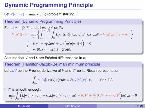
Dynamic Programming PrincipleLet V[mτ ](τ) = minv J(τ, v) (problem starting τ ).
Theorem (Dynamic Programming Principle)
For all τ ∈ [0, T] and all mτ ≥ 0 on R:
V[mvτ ](τ) = min
v
{∫ τ+δτ
τ
∫R
L[mv(t, ·)](t, x, vt)mv(t, x)dxdt + V[mvτ+δτ ](τ + δτ)
}{
∂tmv − σ2
2 ∆mv + div(
mvg[mv](v))
= 0
mv(0, x) = m0(x) given.
Assume that V and L are Fréchet differentiable in m.
Theorem (Hamilton-Jacobi-Bellman minimum principle)
Let ∂mV be the Fréchet derivative of V and V ′ be its Riesz representation:∫Rd
V ′[m](τ)(x)ν(x)dx = ∂mV[m](τ) · ν, ∀ν ∈ L2.
If V ′ is smooth enough,
minv
∫R
(L[mv
τ ](x, τ, v) + ∂mL[mvτ ](x, τ, v) · mv
τ + ∂τV ′ + σ2
2 ∂xxV ′ + v · ∂xV ′)
mvτdx = 0
M. Laurière DPP for MFC 7 / 29

Proof of HJB min. principle (formal) 1/2
A first order approximation of the time derivative in the FP eq. yields:
δτm := mτ+δτ − mτ = δτ
[σ2
2∆mτ − div(vτmτ )
]+ o(δτ). (1)
As V is assumed to be smooth, we have :
V[mτ+δτ ](τ + δτ) = V[mτ ](τ) + ∂τV[mτ ](τ)δτ + ∂mV[mτ ](τ) · δτm + o(δτ). (2)
Then, by Bellman’s principle
V[mτ ](τ) ' minv
{δτ
∫Rd
L[mτ ]mτdx+V[mτ ](τ)+∂τV[mτ ](τ)δτ + ∂mV[mτ ](τ)·δτm}. (3)
Divided by δτ and combined with (1), letting δτ → 0 gives
0 = minv
{∫Rd
L[mτ ]mτdx + ∂τV[mτ ](τ) + ∂mV[mτ ](τ) ·[σ2
2∆mτ − div(vτmτ )
]}. (4)
To finalize the proof we need to relate V to ∂mV.
M. Laurière DPP for MFC 8 / 29

Proof of HJB min. principle (formal) 2/2
PropositionLet (v, m) denote an optimal solution to the problem starting from mτ at time τ . Then:∫
RdV ′[mτ ](τ)mτdx = V[mτ ](τ) +
∫ T
τ
∫Rd
(∂mL[mt](x, t, v) · mt
)mtdxdt
+
∫Rd
(∂mh[mT ](x) · mT
)mT dx.
Differentiating with respect to τ leads to
∂τV[mτ ](τ) =
∫Rd∂τV ′[mτ ](τ)mτdx +
∫Rd
(∂mL[mτ ](x, τ, vτ ) · mτ
)mτdx,
where vτ is the optimal control at time τ . Now, let us use (4), rewritten as
0 = minuτ
{∫Rd
(L[mτ ](x, τ, uτ (x)) + ∂mL[mτ ](x, τ, uτ (x)) · mτ
)mτdx
+
∫Rd
(∂τV ′[mτ ](τ)mτ + V ′[mτ ](τ)
[σ2
2∆mτ − div(uτmτ )
])dx}.
Integrating by parts the last term concludes the proof.M. Laurière DPP for MFC 9 / 29

Outline
1 Mean field control and mean field games
2 Dynamic programming for MFCDynamic programming principleLink with calculus of variations
3 Numerical example 1: oil production
4 Numerical example 2: Bertrand equilibrium
5 Conclusion
M. Laurière DPP for MFC 9 / 29

Dynamic Programming in a specific setting
minv
∫R
(L[mτ ](x, τ, v) + ∂mL[mτ ](x, τ, v) · mτ+∂τV ′ + σ2
2 ∂xxV ′ + v · ∂xV ′)
mτdx = 0
Assume L = L(x, t, v,mt(x), χ(t)) with χ(t) =
∫Rd
h(x, t, v(x, t),mt(x))mt(x)dx.
Then for all ν ∈ L2 :
∂mL[mt](x, t, u) · ν = ∂mL ν +(∫
Rd∂χL ν dx
)h +
(∫Rd∂χL mt dx
)ν ∂mh.
In particular, for ν = mt we have :
∂mL[mt](x, t, u) · mt = ∂mL mt +(∫
Rd∂χL mt dx
)(h + mt ∂mh).
Thus, for optimal v and m,
∂tV ′ +σ2
2∂xxV ′ + v · ∂xV ′ = −
[L + m ∂mL + (h + m ∂mh)
∫Rd∂χL m dx
]where ∂mL, ∂χL, and ∂mh are partial derivatives in the classical sense.
M. Laurière DPP for MFC 10 / 29

Link with calculus of variations
Recall: L = L(x, t, v,mt(x), χ(t)) with χ(t) =
∫Rd
h(x, t, v(x, t),mt(x))mt(x)dx.
Theorem (calculus of variations)v and m are optimal only if for all t and v,∫
Rd
(∂vL + ∂vh
∫Rd∂χL m dy + ∂xm∗
)(v− v)m dx ≥ 0
where m∗ satisfies
∂tm∗ +σ2
2∂xxm∗ + v · ∂xm∗ = −
[L + m ∂mL + (h + m ∂mh)
∫Rd∂χLm dy
]
Link with dynamic programming
V ′ coincides with m∗, the adjoint state of m.
M. Laurière DPP for MFC 11 / 29

Outline
1 Mean field control and mean field games
2 Dynamic programming for MFC
3 Numerical example 1: oil productionThe modelTwo algorithmsNumerical results
4 Numerical example 2: Bertrand equilibrium
5 Conclusion
M. Laurière DPP for MFC 11 / 29
Outline
1 Mean field control and mean field games
2 Dynamic programming for MFC
3 Numerical example 1: oil productionThe modelTwo algorithmsNumerical results
4 Numerical example 2: Bertrand equilibrium
5 Conclusion
M. Laurière DPP for MFC 11 / 29

A (toy) model of oil production5
Setting: continuum of producers exploiting an oil field (limited resource)
Remaining quantity dynamics
dXt = −atdt + σXtdWt, X0 given by its PDF,
• Xt = quantity of oil left in the field at time t (seen by a producer)• atdt = quantity extracted by the producer during (t, t + dt)• W = standard Brownian motion (incertitude), σ > 0 = volatility (constant)• at = a(Xt, t) = feedback law to control the production.
Price
• C = cost of extraction = C(a) = αa + βa2 where: α > 0 and β > 0.• pt = κe−bt(E(at))
−c = price of oil, where: κ > 0, b > 0 and c > 0.
Intuition: p decreases with mean production and time because• scarcity of oil increases its price and conversely.• future oil will be cheaper because it will be replaced by renewable energy.
5[Guéant-Lasry-Lions]
M. Laurière DPP for MFC 12 / 29

Optimisation
Goal:Maximise over a(·, ·) ≥ 0 the profit:
J(a) = E[∫ T
0(ptat − C(at))e−rtdt
]− γ E[|XT |η]
subj to: dXt = −atdt + σXtdWt, X0 given
with γ and η = penalisation parameters (encouraging to consume before T).
Replacing p and C by their expressions gives
J(a) = E[∫ T
0(κe−bt(E[at])
−cat − αat − β(at)2)e−rtdt
]− γ E[|XT |η]
Remark: J = mean of a function of E[at] so it is a MFC problem
M. Laurière DPP for MFC 13 / 29

Remarks on Existence of Solutions
Sufficient condition
if c < 1 and at upper bounded on [0, T], J(a) ≤∫ T
0(cα+ (1 + c)βat)
ate−rt
1− cdt ≤ C.
A counter example: if c > 1 and at = |τ − t| for some τ ∈ (0, T), then the problem isnot well posed (nobody extract oil⇒ infinite price)
Linear feedback caseAssume a(x, t) = w(t)x. Then there is an analytical solution:
Xt = X0 exp(−∫ t
0w(τ)dτ − σ2
2t + σ(Wt −W0)
).
For η = 2, the problem reduces to maximizing over wt = w(t)e−∫ t
0 w(τ)dτ ≥ 0
J(wt) =
∫ T
0
(κe−bt E[X0]
1−cw1−ct − αE[X0]wt − β E[X2
0 ]w2t eσ
2t)e−rtdt
− γ E[X20 ]eσ
2T−2∫ T
0 w(τ)dτ
M. Laurière DPP for MFC 14 / 29

Outline
1 Mean field control and mean field games
2 Dynamic programming for MFC
3 Numerical example 1: oil productionThe modelTwo algorithmsNumerical results
4 Numerical example 2: Bertrand equilibrium
5 Conclusion
M. Laurière DPP for MFC 14 / 29

Dynamic ProgrammingLet u = −a = depletion rate (control).Ignore the constraints on Xt ∈ [0, L] and u ≤ 0: let Xt, ut ∈ R (see the numerical results)
Fokker-Planck eq. for ρ(·, t) = density of Xt
∂tρ−σ2
2∂xx(x2ρ)
+ ∂x(ρu)
= 0 (x, t) ∈ R× (0, T), ρ|t=0 = ρ0 (FP)
Minimise, subject to (FP) with ρ|t=τ = ρτ ,
J(τ, ρτ , u) =
∫ T
τ
∫R
(κe−bt(−ut)
−cut − αut + βu2t
)e−rtρtdxdt +
∫Rγ|x|ηρ|T(x)dx
DPP for V[ρτ ](τ) = minu J(τ, ρτ , u)
u(x, t) =1
2β
[α− ert∂xV ′ − κ(1− c)e−bt(−u)−c
](EU)
∂tV ′ +σ2x2
2∂xxV ′ =
e−rt
4β
(α− ert∂xV ′ − κ(1− c)e−bt(−u)−c
)2(DV)
(depends only on u and not on u)
M. Laurière DPP for MFC 15 / 29

Dynamic ProgrammingLet u = −a = depletion rate (control).Ignore the constraints on Xt ∈ [0, L] and u ≤ 0: let Xt, ut ∈ R (see the numerical results)
Fokker-Planck eq. for ρ(·, t) = density of Xt
∂tρ−σ2
2∂xx(x2ρ)
+ ∂x(ρu)
= 0 (x, t) ∈ R× (0, T), ρ|t=0 = ρ0 (FP)
Minimise, subject to (FP) with ρ|t=τ = ρτ ,
J(τ, ρτ , u) =
∫ T
τ
∫R
(κe−bt(−ut)
−cut − αut + βu2t
)e−rtρtdxdt +
∫Rγ|x|ηρ|T(x)dx
DPP for V[ρτ ](τ) = minu J(τ, ρτ , u)
u(x, t) =1
2β
[α− ert∂xV ′ − κ(1− c)e−bt(−u)−c
](EU)
∂tV ′ +σ2x2
2∂xxV ′ =
e−rt
4β
(α− ert∂xV ′ − κ(1− c)e−bt(−u)−c
)2(DV)
(depends only on u and not on u)M. Laurière DPP for MFC 15 / 29

Fixed point Algorithm
Algorithm 1: Fixed point iteration (parameter ω ∈ (0, 1))
INITIALIZE: set u = u0, i = 0REPEAT:
• Compute ρi by solving (FP)
• Compute ui =
∫R
uiρi
• Compute V ′i by (DV)• Compute ui+1 by (EU) and set ui+1 = ui + ω(ui+1 − ui)
• Set i = i + 1
WHILE not converged.
Open questions:
• (FP) eq.: existence of solution ?
• relevant stopping criteria ? (compare with Riccati, see later)
• 2nd order term vanishes at x = 0. Model does not impose u(0, t) = 0⇒ singularity
M. Laurière DPP for MFC 16 / 29

Calculus of Variations on the Deterministic Ctrl Pb
Introduce an adjoint ρ∗ satisfying: ρ∗|T = γ|x|η, and in R× (0, T)
∂tρ∗ +
σ2x2
2∂xxρ
∗ + u∂xρ∗ = e−rt(α− βu− κ(1− c)e−bt(−u)−c)u (Adj)
ThenGradu J = −
(e−rt(α− 2βu− κ(1− c)e−bt(−u)−c)− ∂xρ
∗)ρ (DJ)
Algorithm 2: Steepest descent (parameter 0 < ε� 1)
INITIALIZE: a = a0 and i = 0REPEAT:• Compute ρi by (FP) with ρi|t=0 given• Compute ui =
∫R uiρidx
• Compute ρ∗i by (Adj)• Compute Gradu J by (DJ)• Compute a feasible descent step µi ∈ R by Armijo rule• Set ui+1 = ui − µiGradu J, i = i + 1
WHILE (‖Gradu J‖ > ε)
Remark: the asymptotic behaviour of u as x→∞ can be an issue
M. Laurière DPP for MFC 17 / 29

Riccati Equation when η = 2
Let η = 2, look for V ′ in the form:
V ′(x, t) = P(t)x2 + Z(t)x + S(t)
Let Qt = ertPt and µ = σ2 − r. For βertµ− Qt > 0, (DV) leads to
Pt =4βµγe(T−t)µ
γe(T−t)µ − γ + 4βµ.
Then:• u is found by (EU):
u(x, t) =1
2β
[α− ert∂xV ′ − κ(1− c)e−bt(−u)−c
](EU)
• in particular ∂xu = − 18β ∂xxV ′ = − 1
4βPt
• but the Fokker-Planck eq. must be solved numerically to compute u.
Remark:• we can also identify Z and S
• u(·, t) : x 7→ 2xP(t) + Z(t) is not a linear feedback
M. Laurière DPP for MFC 18 / 29

Outline
1 Mean field control and mean field games
2 Dynamic programming for MFC
3 Numerical example 1: oil productionThe modelTwo algorithmsNumerical results
4 Numerical example 2: Bertrand equilibrium
5 Conclusion
M. Laurière DPP for MFC 18 / 29

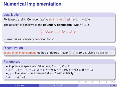
Numerical implementation
LocalisationFix large L and T. Consider (x, t) ∈ (0, L)× (0, T) with ρ(L, t) = 0, ∀t.
The solution is sensitive to the boundary conditions. When η = 2,
12σ2x2∂xV ′ = σ2x3Pt = σ2xV ′
⇒ use this as boundary condition for V ′
Discretizationspace-time finite element method of degree 1 over (0, L)× (0, T). Using freefem++.
Parameters• 50 points in space and 50 in time, L = 10, T = 5• α = 1, β = 1, γ = 0.5, κ = 1, b = 0.1, r = 0.05, σ = 0.5 and c = 0.5• ρ0 = Gaussian curve centred at x = 5 with volatility 1• u0 = −α/(2β)
M. Laurière DPP for MFC 19 / 29

Numerical Implementation: Fixed point AlgoNon-linearity of eq. (DV): semi-linearise it using the iterative loopStopping criteria: error ‖u− ue‖, ue = local min from Ricatti eq. Parameter ω = 0.5.
Optimal u(x, t) and the Ricatti solution slightly below PDF of resource Xt : ρ(x, t)
Remarks: • optimal control is linear• resource distribution: Gaussian to concentrated around x = 0.5
Convergence: error =∫
(∂xu− ∂xue)2dxdt versus k = iteration number :
k 1 2 3 4 5 6 7 8 9 10Error 1035 661.2 8.605 44.7 3.27 0.755 0.335 0.045 0.015 0.003
M. Laurière DPP for MFC 20 / 29

Numerical Implementation: Fixed point Algo (2)
Evolution of production at = −ut and price pt = κe−bt(−ut)−c.
0.04
0.05
0.06
0.07
0.08
0.09
0.1
0.11
0.12
0.13
0 0.5 1 1.5 2 2.5 3 3.5 4 4.5 5time
Production versus time
2.85
2.9
2.95
3
3.05
3.1
0 0.5 1 1.5 2 2.5 3 3.5 4 4.5 5time
Price versus time
M. Laurière DPP for MFC 21 / 29

Numerical Implementation: Steepest DescentGenerates different solutions depending on u0:• u0 = ue: small oscillations to decrease the cost function⇒ mesh dependent• u0 = −0.5: solution below after 10 iterations
Another solution u The corresponding ρ
Convergence: Values of J and ‖Gradu J‖ versus iteration number k
k 0 1 2 3 .. 9J 0.7715 0.2834 0.2494 0.1626 0.0417
‖Gradu J‖ 0.003395 0.001602 0.000700 0.000813 0.000794
M. Laurière DPP for MFC 22 / 29

Linear Feedback Solution
Steepest descent with:• Automatic differentiation (operator overloading in C++)• Initializing with the linear part of the Riccati solution• Gives w(t), very close to the Riccati solution.
Why Ricatti solution is not the best solution?Plot Jd(λ) = J(wd
t + λht), λ ∈ (−0.5,+0.5), ht is an approximate wt −GradJ(wdt ).
0.25
0.3
0.35
0.4
0.45
0.5
0.55
0.6
0.65
0 0.5 1 1.5 2 2.5 3 3.5 4 4.5 5-50
0
50
100
150
200
250
300
350
400
450
-0.5 -0.4 -0.3 -0.2 -0.1 0 0.1 0.2 0.3 0.4 0.5-0.04
-0.02
0
0.02
0.04
0.06
0.08
0.1
0.1 0.12 0.14 0.16 0.18 0.2
Left: w(t) maximizing J(w) VS feedback coef. of the Ricatti solution (solid line)Center: Jd
λ as a function of λ ∈ (−0.5,+0.5); Ricatti solution at λ = 0Right: zoom at λ = ±0.12: absolute min of Jd(.) (shallow and mesh dependent).
M. Laurière DPP for MFC 23 / 29

Outline
1 Mean field control and mean field games
2 Dynamic programming for MFC
3 Numerical example 1: oil production
4 Numerical example 2: Bertrand equilibrium
5 Conclusion
M. Laurière DPP for MFC 23 / 29

Example : Bertrand Equilibrium6
Continuum of producers, whose state is the amount of resource ∈ R+:
dXt = −q(Xt, t)dt + σdWt, ∀t ∈ [0, T],
if Xt > 0 and Xt is absorbed at 0, X0 has density m0,
where q(x, t) = a(η(t))[1 + εp(t)
]− p(x, t) is the quantity produced, with
η(t) =
∫R+
m(x, t)dx : the proportion of remaining producers,
p(t) =
∫R+
p(x, t)m(x, t)dx : the average price (non local in p),
p(t) : the price (control, same for all the agents).
Last, a(η) = 11+εη , and ε > 0 reflects the degree of interaction.
The goal of a typical agent is to maximise
J (p) = E[∫ T
0e−rsp(s,Xs)q(s,Xs)1{Xs>0}ds
].
6[Chan-Sircar]M. Laurière DPP for MFC 24 / 29

PDE System
Proposition
The optimal control is given : p(x, t) = 12
(a(η(t))[1 + εp(t)] + ∂xu(x, t)
), and the
optimal equilibrium is given by :
q(x, t) =12
αMFTC + ε
∫R+
∂xu(ξ, t)m(ξ, t)dξ
αMFTC + ε
∫R+
m(ξ, t)dξ− ∂xu(x, t)
where αMFTC = 1,
with (u,m) satisfying∂tu(x, t)− ru(x, t) + σ2
2 ∂xxu(x, t) +(ψ(m(·, t), ∂xu(·, t))(x)
)2= 0,
∂tm(x, t)− σ2
2 ∂xxm(x, t)− ∂x
(ψ(m(·, t), ∂xu(·, t))m(·, t)
)(x) = 0,
with ψ(m(·, t), ∂xu(·, t)) : x 7→ q(x, t).
For the corresponding MFG, αMFTC is replaced by αMFG = 2.77[Bensoussan-Graber]
M. Laurière DPP for MFC 25 / 29
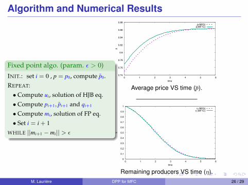
Algorithm and Numerical Results
Fixed point algo. (param. ε > 0)
INIT.: set i = 0 , p = p0, compute p0.
REPEAT:
• Compute ui, solution of HJB eq.
• Compute pi+1, pi+1 and qi+1
• Compute mi, solution of FP eq.
• Set i = i + 1
WHILE ||mi+1 − mi|| > ε
�����
�����
�����
����
�����
�����
�����
�����
�� �� �� � �� � ��
��
�� �
�����������������
Average price VS time (p).
��
����
����
����
����
����
����
���
���
����
��
�� �� �� �� �� �� ��
�
� ��
���������������
Remaining producers VS time (η).M. Laurière DPP for MFC 26 / 29

Outline
1 Mean field control and mean field games
2 Dynamic programming for MFC
3 Numerical example 1: oil production
4 Numerical example 2: Bertrand equilibrium
5 Conclusion
M. Laurière DPP for MFC 26 / 29

Conclusion
Summary:
• dynamic programming for mean field control problems
• two numerical methods
• application to economics
• follow-up articles8
Current directions of research:
• proof of existence and uniqueness for the PDE system
• other numerical methods
• other applications
8[Pham-Wei, Pfeiffer, . . . ]M. Laurière DPP for MFC 27 / 29

Some References (very partial)
� A. Bensoussan, J. Frehse and P. Yam, Mean Field Games and Mean Field TypeControl Theory, Springer Briefs in Mathematics, Springer, New York (2013)
� R. Carmona, F. Delarue and A. Lachapelle, Control of McKean-Vlasov dynamicsversus Mean Field Games, Math. Financ. Econ., 7, 131–166 (2013)
� P. Chan and R. Sircar, Bertrand and Cournot mean field games, Appl. Math. Optim.,71(3):533–569 (2015)
� O. Guéant, J.-M. Lasry and P.-L. Lions, Mean Field Games and Applications, inParis-Princeton Lectures on Mathematical Finance 2010, Springer (2011)
� M. Laurière and O. Pironneau, Dynamic programming for mean-field type control, J.Optim. Theory Appl., 169(3):902–924 (2016) (see also C.R.A.S., 2014)
� L. Pfeiffer, Numerical methods for mean-field type optimal control problems, Pureand Applied Functional Analysis, 1(4):629–65 (2016)
� H. Pham and X. Wei, Dynamic programming for optimal control of stochasticMcKean-Vlasov dynamics, SIAM Journal on Control and Optimization, to appear.
M. Laurière DPP for MFC 28 / 29

Thank you !
M. Laurière DPP for MFC 29 / 29