dynamic simulation and optimization using · pdf filedynamic simulation and optimization using...
TRANSCRIPT
1
Dynamic Simulation and Optimization using EMSO
Argimiro R. Secchi
– Lecture 5 –Simulation of tubular reactors.
Solutions for Process Control and OptimizationPEQ/COPPE-UFRJ
January, 2013
2
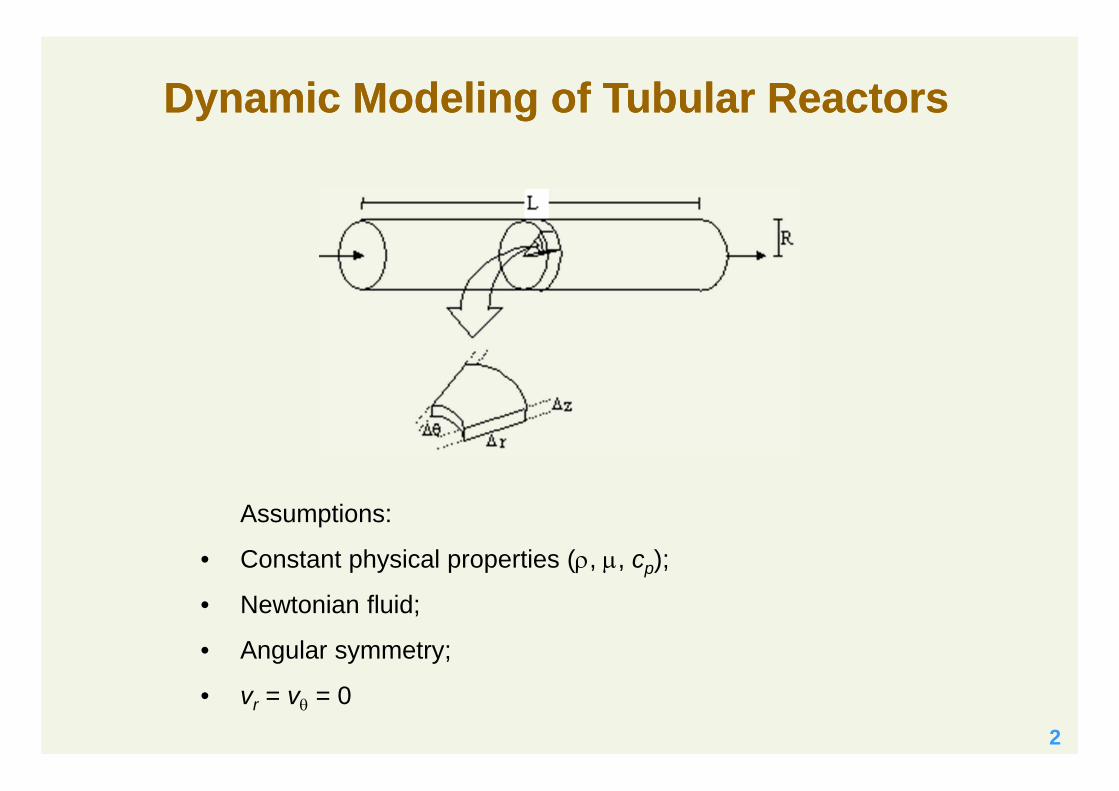
Dynamic Modeling of Tubular ReactorsDynamic Modeling of Tubular Reactors
Assumptions:
• Constant physical properties (, , cp);
• Newtonian fluid;
• Angular symmetry;
• vr = v = 0

3
Model classification based on physical-chemistry principles
Microscopic Model
Multiple Gradients Model
Maximum Gradient Model
Macroscopic Model

4
Microscopic Model
( )( , ) ( ) ( D )li iz i i i
C Cv r t C v C Rt z
( ) ( ) ( ) ( ) ( )( , ) ( ) ( ) ( )l l l t tp p z p v v r
T Tc c v r t c v T k T St z
( ) 2[ ] lv v v v v P v gt
( ) ( )t ti i iv c J C D
( ) ( )t tpc v T q k T
( ) ( )t tv v v
Turbulence Model (simple example):
( . ) 0v v v r tz z ( , )
Computational Fluid Dynamic (CFD)
5
Recommended Numerical MethodRecommended Numerical Method
Finite Volume:Consist in carry out balances of properties in elementary volumes (finite volumes), or in an equivalent form in the integration over the elementary volume of the differential equation in the conservative form (or divergent form, where the fluxes appearing in the derivatives).
Use of CFD software (Computational Fluid Dynamics)
6
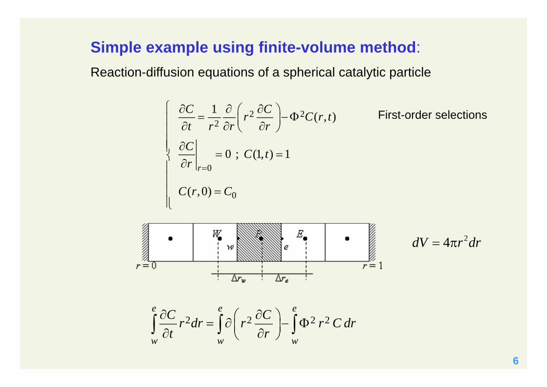
Simple example using finite-volume method:Reaction-diffusion equations of a spherical catalytic particle
2 22
0
0
1 ( , )
0 ; (1, ) 1
( ,0)
r
C Cr C r tt r r rC C tr
C r C
2 2 2 2e e e
w w w
C Cr dr r r C drt r
First-order selections
24dV r dr
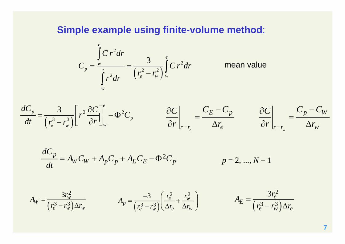
7
2
22 2
2
3
e
ew
p ewe w
w
C r drC C r dr
r rr dr
2 2
3 3
3 ep
pwe w
dC Cr Cdt rr r
mean value
e w
E p p W
e wr r r r
C C C CC Cr r r r
2pW W p p E E p
dCA C A C A C C
dt
2
3 33 w
We w w
rAr r r
2 2
3 33 e w
pe we w
r rAr rr r
2
3 33 e
Ee w e
rAr r r
p = 2, ..., N 1
Simple example using finite-volume method:
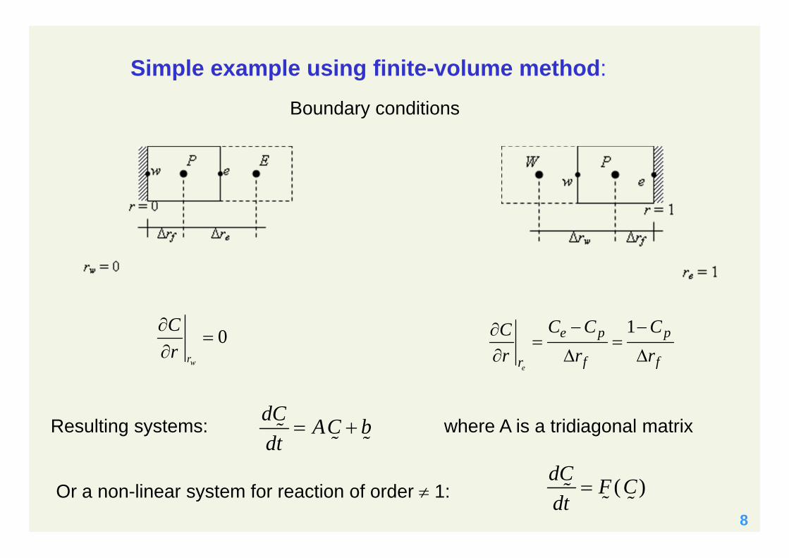
8
0wr
Cr
1
e
e p p
f fr
C C CCr r r
dC AC bdt
Resulting systems: where A is a tridiagonal matrix
Boundary conditions
( )dC F Cdt
Or a non-linear system for reaction of order 1:
Simple example using finite-volume method:

9
Multiple Gradients Model
( , ) ( D )i iz i i
C Cv r t C Rt z
( , ) ( )p p z v rT Tc c v r t k T St z
( ) ( )t l D D D( ) ( )t lk k k ( ) ( )t l
2zz
v P v gt
Boundary Conditions:
reaction zonevz, Ci0, T0
z = 0 z = Lz = 0 ¯ z = 0+ z = L¯ z = L+
10
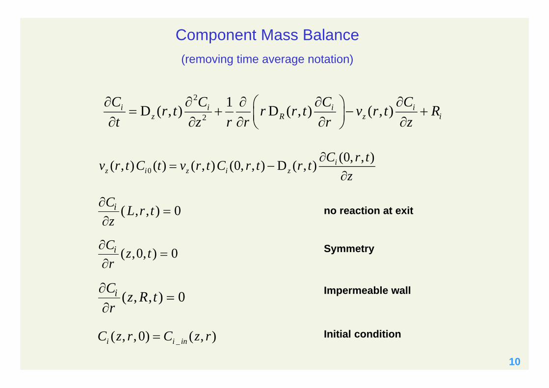
2
2
1D ( , ) D ( , ) ( , )i i i iz R z i
C C C Cr t r r t v r t Rt z r r r z
0(0, , )( , ) ( ) ( , ) (0, , ) D ( , ) i
z i z i zC r tv r t C t v r t C r t r t
z
Cz
L r ti ( , , ) 0
Cr
z ti ( , , )0 0
Cr
z R ti ( , , ) 0
_( , , 0) ( , )i i inC z r C z r
no reaction at exit
Symmetry
Initial condition
Impermeable wall
Component Mass Balance(removing time average notation)
11
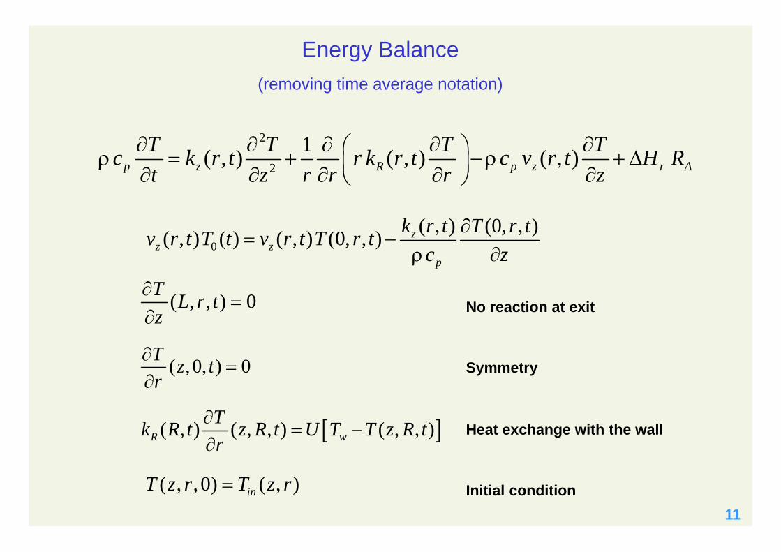
( , , ) 0T L r tz
( ,0, ) 0T z tr
( , , 0) ( , )inT z r T z r
No reaction at exit
Symmetry
Initial condition
Heat exchange with the wall
2
2
1( , ) ( , ) ( , )p z R p z r AT T T Tc k r t r k r t c v r t H Rt z r r r z
0( , ) (0, , )( , ) ( ) ( , ) (0, , ) z
z zp
k r t T r tv r t T t v r t T r tc z
( , ) ( , , ) ( , , )R wTk R t z R t U T T z R tr
Energy Balance(removing time average notation)
12
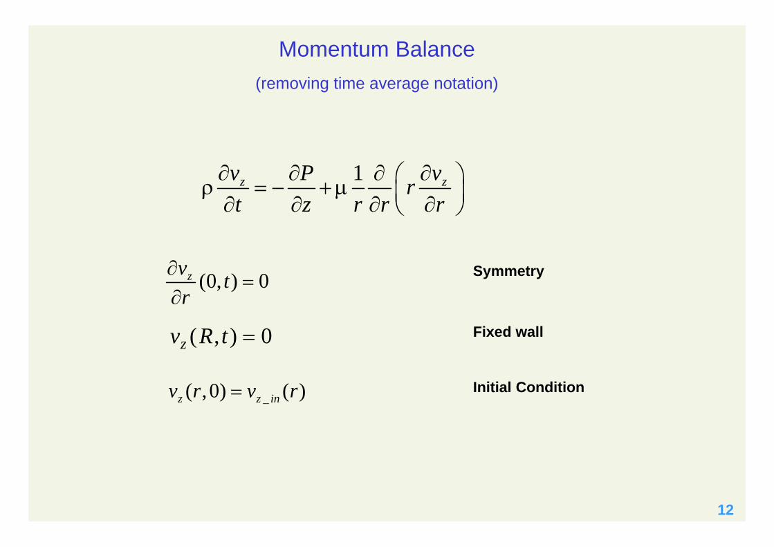
(0, ) 0zv tr
_( ,0) ( )z z inv r v r
Symmetry
Initial Condition
Fixed wall
1z zv P vrt z r r r
v R tz ( , ) 0
Momentum Balance(removing time average notation)
13
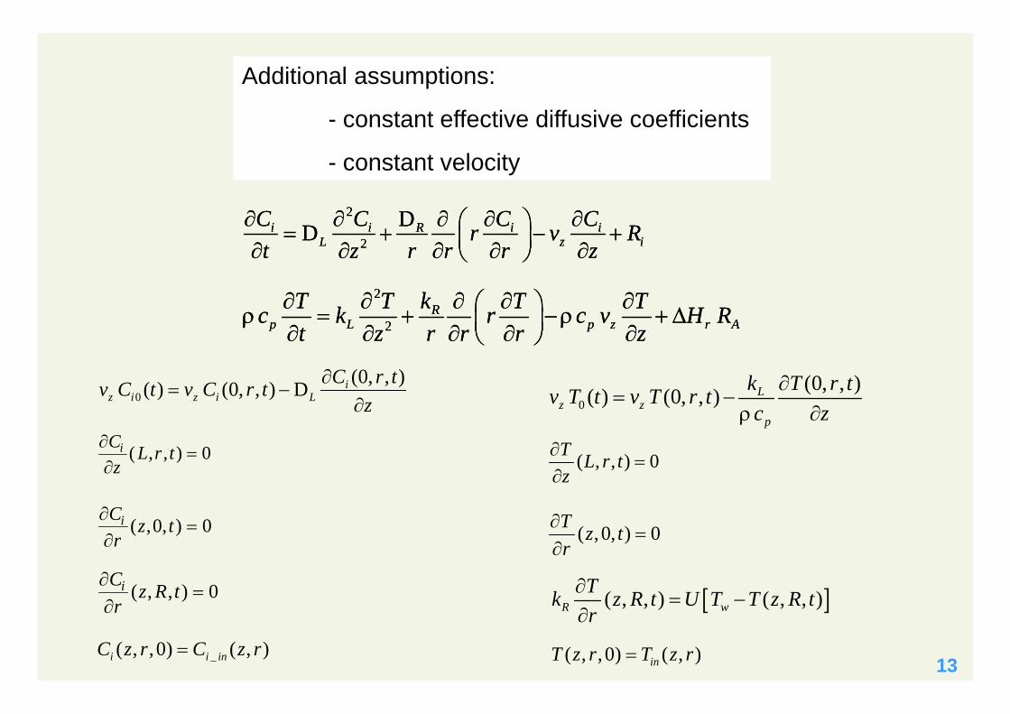
2
2
DDi i i iRL z i
C C C Cr v Rt z r r r z
2
2R
p L p z r AT T k T Tc k r c v H Rt z r r r z
Additional assumptions:
- constant effective diffusive coefficients
- constant velocity
( , , ) 0T L r tz
( ,0, ) 0T z tr
( , , 0) ( , )inT z r T z r
0(0, , )( ) (0, , ) L
z zp
k T r tv T t v T r tc z
( , , ) ( , , )R wTk z R t U T T z R tr
0(0, , )( ) (0, , ) D i
z i z i LC r tv C t v C r t
z
Cz
L r ti ( , , ) 0
Cr
z ti ( , , )0 0
Cr
z R ti ( , , ) 0
_( , ,0) ( , )i i inC z r C z r
2
2
DDi i i iRL z i
C C C Cr v Rt z r r r z
2
2R
p L p z r AT T k T Tc k r c v H Rt z r r r z
14
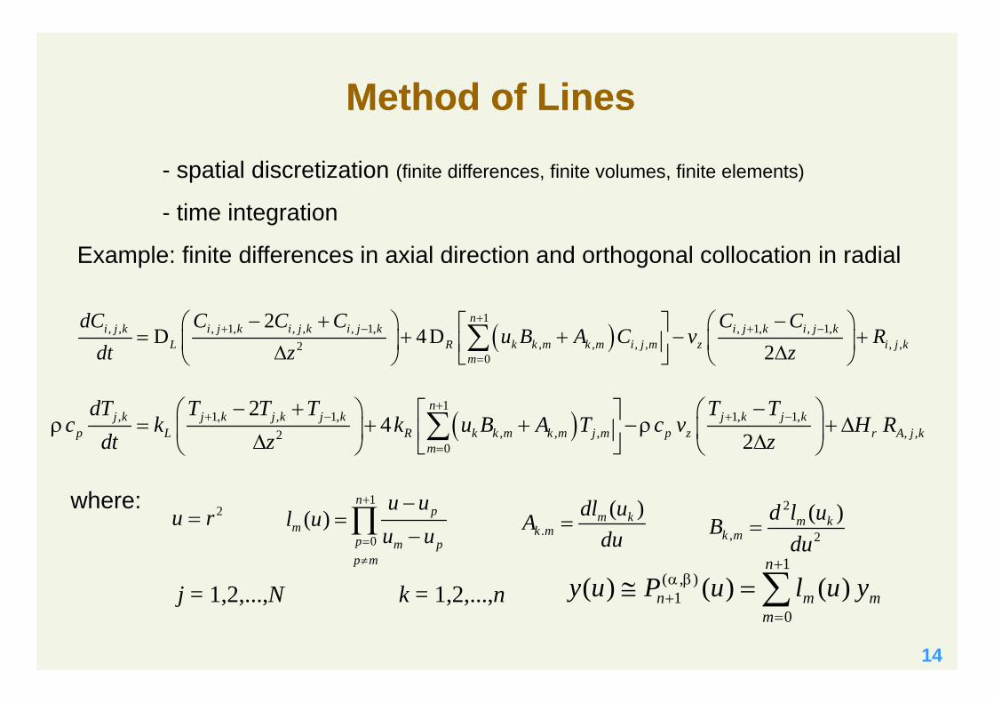
Method of LinesMethod of Lines
- spatial discretization (finite differences, finite volumes, finite elements)
- time integration
Example: finite differences in axial direction and orthogonal collocation in radial
1
, , , 1, , , , 1, , 1, , 1,, , , , , ,2
0
2D 4 D
2
ni j k i j k i j k i j k i j k i j k
L R k k m k m i j m z i j km
dC C C C C Cu B A C v R
dt z z
1
, 1, , 1, 1, 1,, , , , ,2
0
24
2
nj k j k j k j k j k j k
p L R k k m k m j m p z r A j km
dT T T T T Tc k k u B A T c v H R
dt z z
.( )m k
k mdl uA
du
2
, 2
( )m kk m
d l uBdu
1
0( )
np
mp m pp m
u ul u
u u
2u rwhere:
j = 1,2,...,N k = 1,2,...,n1
( , )1
0( ) ( ) ( )
n
n m mm
y u P u l u y

15
,2, 00 ,1,
( )( ) D
2i k i
z i z i k L
C C tv C t v C
z
, 1, , , 0i N k i N kC C
1
0, , ,0
0n
m i j mm
A C
1
1, , ,0
0n
n m i j mm
A C
, , _ , ,i j k i in j kC C
Method of LinesMethod of Lines
Boundary conditions
1, , 0N k N kT T
1
0, ,0
0n
m j mm
A T
, , ,j k in j kT T
2, 00 1,
( )( )
2kL
z z kp
T T tkv T t v Tc z
1
1, , , 10
n
R n m j m w j nm
k A T U T T
j = 1,2,...,N k = 1,2,...,n
Results in a DAE system!

16
Another Multiple Gradients Model(ignoring radial gradients) – PFR with axial dispersion
2
2Di i iL z i
C C Cv Rt z z
2
2
2p L p z w r A
T T T Uc k c v T T H Rt z z R
0(0, )( ) (0, ) D i
z i z i LC tv C t v C t
z
( , ) 0iC L tz
_( ,0) ( )i i inC z C z
( , ) 0T L tz
( ,0) ( )inT z T z
0(0, )( ) (0, ) L
z zp
k T tv T t v T tc z
0
0
( , , )( , )
R
i
i R
C r z t r drC z t
r dr
0
0
( , , )( , )
R
R
T r z t r drT z t
r dr

17
, , 1 , , 1 , 1 , 1,2
2D
2i j i j i j i j i j i j
L z i j
dC C C C C Cv R
dt z z
1 1 1 1,2
2 22
j j j j j jp L p z w j r A j
dT T T T T T Uc k c v T T H Rdt z z R
j = 1,2,...,N
,2 00 ,1
( )( ) D
2i i
z i z i L
C C tv C t v C
z
, 1 , 0i N i NC C
, _ ,i j i in jC C
1 0N NT T
,j in jT T
2 00 1
( )( )2
Lz z
p
T T tkv T t v Tc z
Method of LinesMethod of Lines
- spatial discretization (F.D., F.V., orthogonal collocation on finite elements)
- time integration
Example: finite differences in axial direction
18
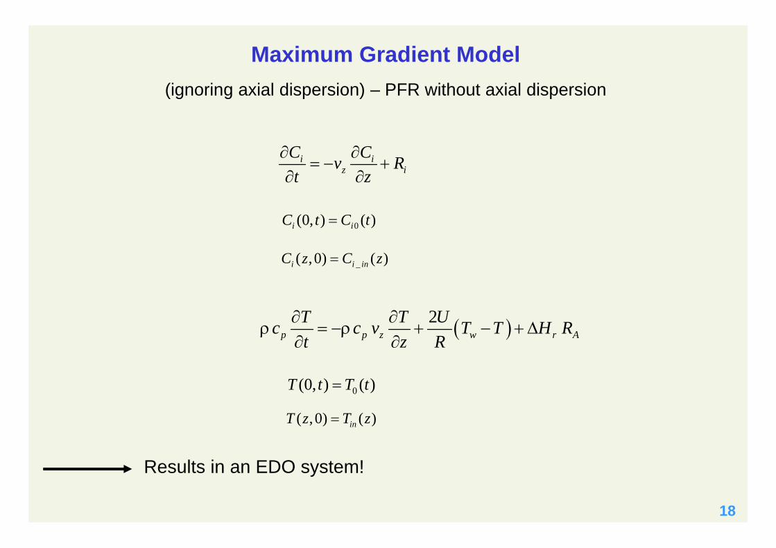
Maximum Gradient Model(ignoring axial dispersion) – PFR without axial dispersion
i iz i
C Cv Rt z
2p p z w r A
T T Uc c v T T H Rt z R
0(0, ) ( )i iC t C t
_( ,0) ( )i i inC z C z
( ,0) ( )inT z T z
0(0, ) ( )T t T t
Results in an EDO system!

19
Macroscopic Model
0 ( )ii z i z i
dCV C t v S C v S R Vdt
0 ( ) ( )p p z p z t w r AdTc V c v S T t c v S T U A T T H R Vdt
_(0)i i inC C
(0) inT T
0
0
( , )( )
L
i
i L
C z t S dzC t
S dz
0
0
( , )( )
L
L
T z t S dzT t
S dz
Results in a EDO system!
20
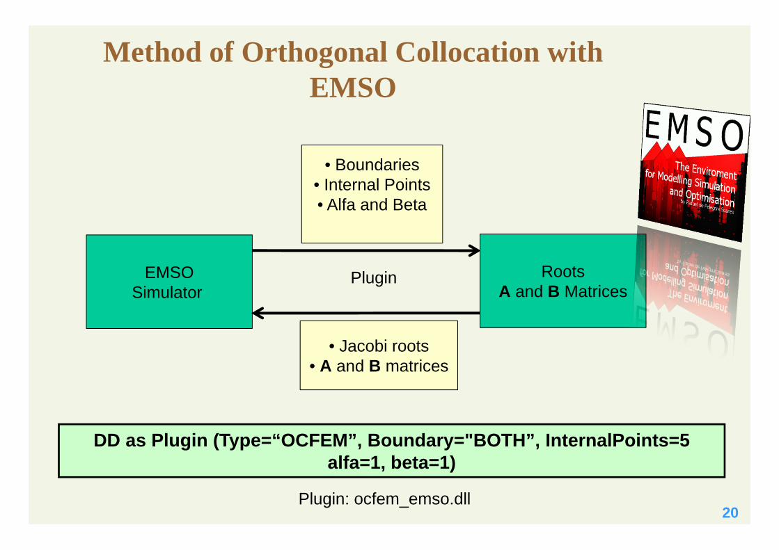
Method of Orthogonal Collocation with EMSO
EMSOSimulator
RootsA and B Matrices
• Boundaries• Internal Points• Alfa and Beta
• Jacobi roots• A and B matrices
Plugin
DD as Plugin (Type=“OCFEM”, Boundary="BOTH”, InternalPoints=5 alfa=1, beta=1)
Plugin: ocfem_emso.dll
21
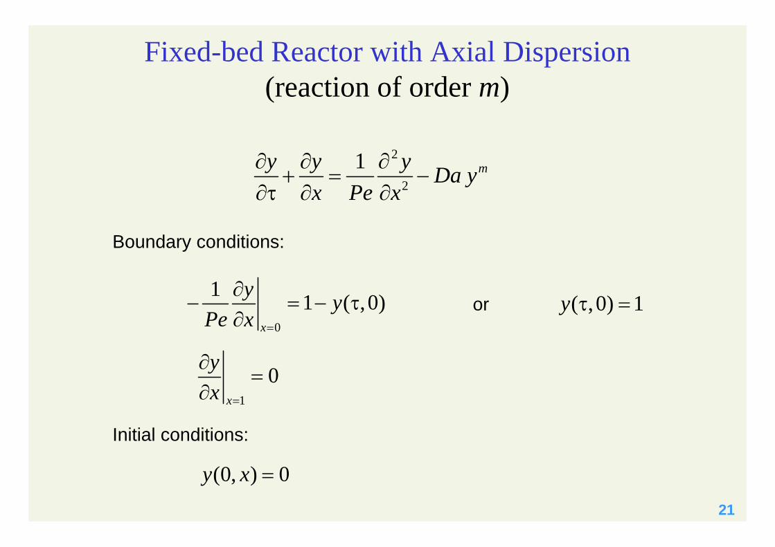
Fixed-bed Reactor with Axial Dispersion(reaction of order m)
2
2
1 my y y Da yx Pe x
Boundary conditions:
0
1 1 ( ,0)x
y yPe x
1
0x
yx
( ,0) 1y or
Initial conditions:
(0, ) 0y x
22
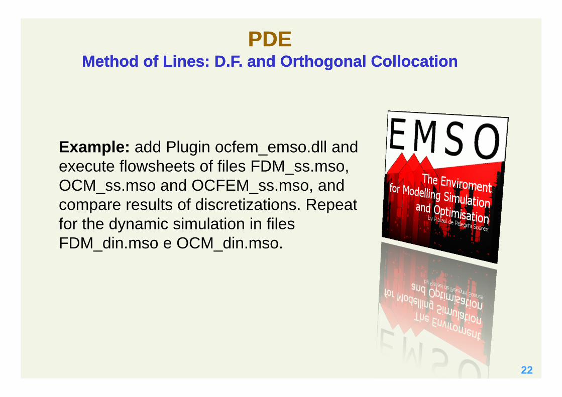
Example: add Plugin ocfem_emso.dll and execute flowsheets of files FDM_ss.mso, OCM_ss.mso and OCFEM_ss.mso, and compare results of discretizations. Repeat for the dynamic simulation in files FDM_din.mso e OCM_din.mso.
PDEMethod of Lines: D.F. and Orthogonal Collocation
PDEMethod of Lines: D.F. and Orthogonal Collocation
23
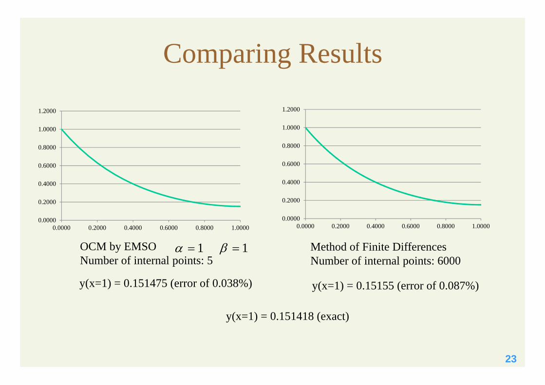
Comparing Results
OCM by EMSONumber of internal points: 5
y(x=1) = 0.151475 (error of 0.038%)
1 1
0.0000
0.2000
0.4000
0.6000
0.8000
1.0000
1.2000
0.0000 0.2000 0.4000 0.6000 0.8000 1.00000.0000
0.2000
0.4000
0.6000
0.8000
1.0000
1.2000
0.0000 0.2000 0.4000 0.6000 0.8000 1.0000
Method of Finite DifferencesNumber of internal points: 6000
y(x=1) = 0.15155 (error of 0.087%)
y(x=1) = 0.151418 (exact)
24
Case Study
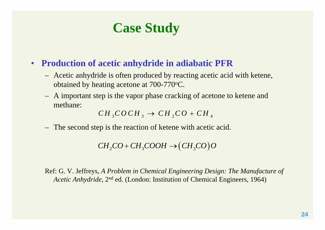
• Production of acetic anhydride in adiabatic PFR– Acetic anhydride is often produced by reacting acetic acid with ketene,
obtained by heating acetone at 700-770oC.– A important step is the vapor phase cracking of acetone to ketene and
methane:
– The second step is the reaction of ketene with acetic acid.
Ref: G. V. Jeffreys, A Problem in Chemical Engineering Design: The Manufacture of Acetic Anhydride, 2nd ed. (London: Institution of Chemical Engineers, 1964)
3 3 2 4C H C O C H C H C O C H
2 3 3CH CO CH COOH CH CO O
25
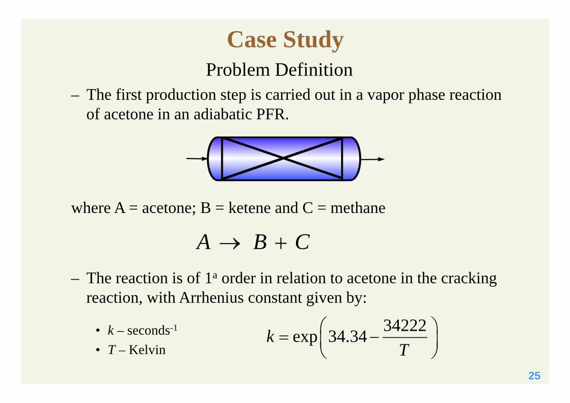
34222exp 34.34kT
Problem Definition – The first production step is carried out in a vapor phase reaction
of acetone in an adiabatic PFR.
where A = acetone; B = ketene and C = methane
– The reaction is of 1a order in relation to acetone in the cracking reaction, with Arrhenius constant given by:
• k – seconds-1
• T – Kelvin
CBA
Case Study
26
Process Description
– Reactor geometry• adiabatic continuous tubular reactor;• bank of 1000 tubes of 1 in sch. 40 with cross section of 0.557 m2;• total length of 2.28 m;
– Operating conditions• feed temperature 762oC (1035 K);• operating pressure: 1.6 atm• feed flow rate of 8000 kg/h (137.9 kmol/h);
– Composition• acetone, ketene and methane• feed of pure acetone
– Kinetics• first order reaction, • pre-exponential factor (k0): 8.2 x 10¹⁴ s-1
• activation energy (E/R): 34222 K• heat of reaction: -80.77 kJ/mol
Case Study
27
Example: run FlowSheet in file PFR_Adiabatico.mso and plot steady-state temperature and composition profiles. Show also the evolution of the temperature profile. Discuss the type and quality of discretization.
Case study– Production of acetic anhydride –
Case study– Production of acetic anhydride –

28
ExerciseExerciseSolve the reaction-diffusion problem in a spherical catalytic particle, given by:
2 2 1/ 22
1y yr yt r r r
0
0r
yr
1( , ) 1
ry t r
0( , ) 0
ty t r
2 (Thiele modulus)
29
ReferencesReferences• Himmelblau, D. M. & Bischoff, K. B., "Process Analysis and Simulation - Deterministic Systems", John Wiley & Sons, 1968.• Finlayson, B. A., "The Method of Weighted Residuals and Variational Principles with Application in Fluid Mechanics, Heat and Mass Transfer", Academic Press, 1972.• Villadsen, J. & Michelsen, M. L., "Solution of Differential Equation Models by Polynomial Approximation", Prentice-Hall, 1978.• Davis, M. E., "Numerical Methods and Modeling for Chemical Engineers", John Wiley & Sons, 1984.• Denn, M., "Process Modeling", Longman, New York, 1986.• Luyben, W. L., "Process Modeling, Simulation, and Control for Chemical Engineers", McGraw-Hill, 1990.• Silebi, C.A. & Schiesser, W.E., “Dynamic Modeling of Transport Process Systems”, Academic Press, Inc., 1992.• Biscaia Jr., E.C. “Método de Resíduos Ponderados com Aplicação em Simulação de Processos”, XV CNMAC, 1992• Ogunnaike, B.A. & Ray, W.H., “Process Dynamics, Modeling, and Control”, Oxford Univ. Press, New York, 1994.• Rice, R.G. & Do, D.D., “Applied Mathematics and Modeling for Chemical Engineers”, John Wiley & Sons, 1995.• Maliska, C.R. “Transferência de Calor e Mecânica dos Fluidos Computacional”, 1995.• Bequette, B.W., “Process Dynamics: Modeling, Analysis, and Simulation”, Prentice Hall, 1998.• Fogler, H.S., “Elementos de Engenharia de Reações Químicas”, Prentice Hall, 1999.

30
For helping in the preparation of this material
Special thanks to
For supporting the ALSOC Project.
Prof. Rafael de Pelegrini Soares, D.Sc.Eng. Gerson Balbueno Bicca, M.Sc.Eng. Euclides Almeida Neto, D.Sc.Eng. Eduardo Moreira de Lemos, D.Sc.Eng. Marco Antônio Müller

31
... thank you for your attention!
Process Modeling, Simulation and Control Lab• Prof. Argimiro Resende Secchi, D.Sc.• Phone: +55-21-2562-8307• E-mail: [email protected]• http://www.peq.coppe.ufrj.br/Areas/Modelagem_e_simulacao.html
http://www.enq.ufrgs.br/alsoc
EP 2013
Solutions for Process Control and Optimization