dynamics of ocean cables with local low-tension regions

Ocean Engng,Vol. 25, No. 6, pp. 443–463, 1998 1998 Elsevier Science Ltd. All rights reservedPergamon Printed in Great Britain

0029–8018/98 $19.00+ 0.00

PII: S0029–8018(97)00020–6

DYNAMICS OF OCEAN CABLES WITH LOCAL LOW-TENSION REGIONS

Yang Sun* and John W. LeonardDepartment of Civil and Environmental Engineering, The University of Connecticut, Storrs, CT 06269,

U.S.A.

(Received7 March 1997;accepted in final form26 March 1997)

Abstract—A general set of 3-D dynamic field equations for a cable segment is derived based onthe classical Euler–Kirchhoff theory of an elastica. The model includes flexural stiffness to removethe potential singularity when cable tension vanishes and can be reduced to the equations for aperfectly flexible cable. A hybrid model and a solution scheme by direct integration are thenproposed to solve the oceanic cable/body system with a localized low-tension region. Numericalexamples demonstrate the capability and validity of the formulation and the numerical algorithm. 1998 Elsevier Science Ltd.

1. INTRODUCTION

The formulations and solution techniques for the dynamics of cables have been success-fully applied to many oceanic cable structures (Wang, 1977; Liu, 1982; Webster and Palo,1982; Delmer and Stephens, 1989; Chiou and Leonard, 1991), they have not, however,served well for cable systems with initial or potential low-tension regions. This is due tothe fact that most models have traditionally assumed that the cable can be treated as aslender, perfectly flexible cylinder. By this assumption, the cable is a load-adaptive elementin that it responds to loads by adapting its equilibrium geometry to carry all applied loadsby tension alone. Consequently, the dynamic equations of motion for the cable becomesingular if the cable loses tension anywhere within the cable scope.

In the simulation of oceanic cable/body deployment and many other cable applications,however, initial or potential low-tension regions may exist. A perfectly flexible cable nearthe touchdown point loses tension completely if a realistic pay-out rate is assumed. Whena lumped body touches the sea floor, a sudden reduction in tension causes the entire systemto slacken. During abrupt maneuvers of a surface vessel or during high speed pay-outof cable, the steep gradient of velocity may cause the cable to lose tension temporarily(Sun, 1996).

In order to remove the singularity from the governing equations when cable tensionbecomes zero, it is intuitively clear that the cable flexural or torsional stiffness should beretained. A study conducted by Triantafyllou and Howell (1992, 1994) by analytical meanson cable dynamic equations of motion under negative tension has provided a theoreticalview of this hypothesis. Burgess (1993) investigated the effects of cable bending stiffness

*Presently with Friede & Goldman Ltd, New Orleans, LA, U.S.A.

443

444 Y. Sun and J. W. Leonard

in the simulation of undersea cable deployment. Bending stiffness is incorporated in thisformulation and a finite difference scheme is used. The study shows that the addition ofa small bending stiffness improves the stability of the solution in a low-tension situation.The study also suggests the necessity of improving the efficiency of the solution schemeby separating the boundary region where the bending stiffness is important from themajority of the cable span.

The objective of the present study is to develop a general set of 3-D dynamic fieldequations and boundary conditions with flexural, torsional and inertia effects included foroceanic cable/body systems. The formulation should be ‘generic’ in that it can be reducedto simplified models, including a traditional perfect flexible cable. This provides the flexi-bility of using different or mixed models in a single software package. An improvementto the approach, similar to that adopted by Triantafyllou and Howell (1992) and Burgess(1993), of adding dependent variables to the equations for flexural responses at every pointalong the cable, will be developed. A more efficient scheme of adding variables only inthe boundary layer region will then be sought.

2. DYNAMIC FIELD EQUATIONS

The mathematical model is comprised of the cable dynamic equations and the boundaryconditions. They are derived based on the following assumptions.

1. The cable material is homogeneous, isotropic and elastic.2. The longitudinal strain is small and defined as

e = limds

0→0

ds 2 ds0

ds0=

dsds0

2 1 (1)

where ds and ds0 are the stretched and unstretched differential lengths of cable seg-ment, respectively.3. The stress-couples are connected with the curvature and twist of the cable by the

‘Bernoulli–Eulerian’ theory (Love, 1944).4. Shear deformation is neglected.5. Cable and body dimensions are small compared to incident wave lengths. Thus, calcu-

lation of hydrodynamic forces by the Morison equation is valid.

The general definition sketch of the cable system is shown in Fig. 1. TheXi (i = 1,2,3)define a fixed Cartesian frame located at the still water surface with unit base vectorse1,e2 and e3 . At an arc length distance,s, measured from the vessel connection point, theunit vectorsa1, a2 and a3 define the unit base vectors of a local coordinate system. Thislocal system remains aligned with the principal axes of the cable cross-section at all pointsalong the cable scope. Thus, as the local coordinate axes ‘travel’ along the cable scope,a3 remains tangent to the cable central-line, whilea1 and a2 rotate about that axis at arate defined by the tortuosity.

Define three Euler anglesf, u andc (see Fig. 2) to describe the rotation transformationbetween the global frame and the local frame. The transformation is accomplished in threeorderly steps:

1. rotateX3 through an anglef to bring X2 into the X3 and a3 plane (0, f , 2p);2. rotate about the newX1 axis through an angleu to align X3 with a3 (0 , u , p);

445Dynamics of ocean cables

Fig. 1. General definition sketch.

Fig. 2. Euler angles representation.

3. rotate about the newX3 axis through an anglec to fix the orientation ofa1 and a2 (0, c , 2p).

The fixed inertia frame is related to the local frame by the three sequential coordi-nate transformations

5a1

a2

a3

6 = LcLuLf5e1

e2

e3

6 (2)


where the three transformation matrices are

Lf = 3 cosf sin f 0

2 sin f cosf 0

0 0 14, Lu = 31 0 0

0 cosu sin u

0 2 sin u cosu4, Lc = 3 cosc sin c 0

2 sin c cosc 0

0 0 14 (3)

Multiplication of the three matrices yields

L = LcLuLf = (4)

3cosf cosc 2 sin f cosu sin c sin f cosc + cosf cosu sin c sin u sin c

2 cosf sin c 2 sinf cosu cosc 2 sin f sinc + cosf cosu cosc sin u cosc

sinf sin u 2 cosf sin u cosu4

The components of angular velocity are determined by

v1 =∂f

∂tsin u sin c +

∂u

∂tcosc

v2 =∂f

∂tsin u cosc 2

∂u

∂tsin c

v3 =∂f

∂tcosu +

∂c

∂t(5)

or in vector form

v = [L]∂x

∂t(6)

wherex = { f, u, c} T and t is the time. The 3× 3 matrix [L] is defined as

[L] = 3sin u sin c cosc 0

sin u cosc 2 sin c 0

cosu 0 14 (7)

Similarly, the local curvature vector can be expressed as

k = [L]∂x

∂s0(8)

Alternatively, by inverting Equation (8) one may write

∂x

∂s0

= [G]k (9)

where [G] is the inverse of the matrix

[G] = [L] 2 1 = 3 cscu sin c cscu cosc 0

cosc 2 sin c 0

2 cot u sin c 2 cot u cosc 14 (10)


Note that Equation (10) becomes singular whenc = np (n = 0,1,2,...), i.e. when thecable is perpendicular to theX1X2 plane. If this situation happens (although it is rare), anadditional rotation about theX1 axis will be necessary.

From vector mechanics for a space curve, one knows that the derivative of a positionvector at a point with respect to the curved length results in the tangent vector at that point:

∂r∂s0

= ea3 (11)

wheree = 1 + e is the cable stretch.Assuming the configuration of the cable is a smooth curve, the sequence of space and

time differentiation of the position vector is interchangeable. Thus, the time derivative ofthe geometric Equation (11) becomes

DvDs0

=DDt

[ea3] (12)

wherev is the velocity vector.Using the chain rule of differentiation and the material derivative of the velocity vector,

one obtains the compatibility equation

∂e

∂ta3 + ev × a3 =

∂v∂s0

+ k × v (13)

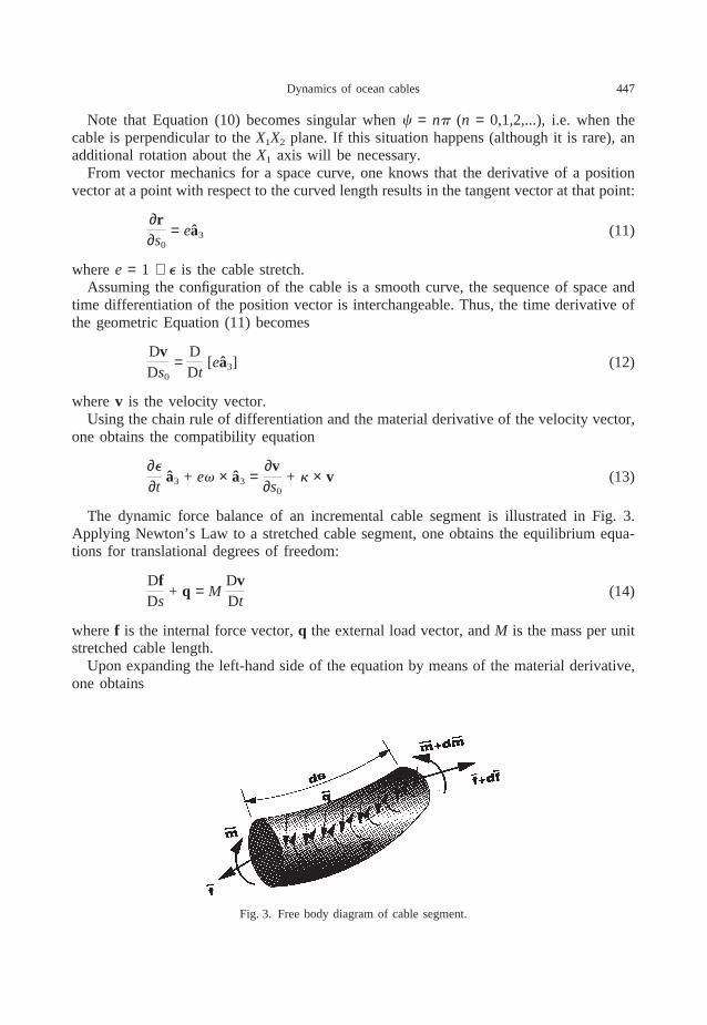
The dynamic force balance of an incremental cable segment is illustrated in Fig. 3.Applying Newton’s Law to a stretched cable segment, one obtains the equilibrium equa-tions for translational degrees of freedom:

DfDs

+ q = MDvDt

(14)

wheref is the internal force vector,q the external load vector, andM is the mass per unitstretched cable length.

Upon expanding the left-hand side of the equation by means of the material derivative,one obtains

Fig. 3. Free body diagram of cable segment.


∂f∂s0

+ k × f + eq = M0F∂v∂t

+ v × v +∂vp

∂ta3 (15)

+ 2vpS∂e

∂ta3 + v × a3D + v2

pS∂e

∂s0a3 + k × a3DG

whereM0 is the mass per unit unstretched length, andvp is the cable pay-out rate.The inertia effects of the pay-out have been included in the above equations by using

the following expression for the total derivative of the velocity vector (Leonard and Karno-ski, 1990; Burgess, 1993; Sun, 1996):

DvDt

=∂v∂t

+ v × v +∂vp

∂ta3 + 2vpS∂e

∂ta3 + v × a3D + v2

pS∂e

∂s0a3 + k × a3D (16)

where the first term on the right-hand side of Equation (16) is the time rate change of themagnitude of the velocity, the second term is the time rate change of the velocity due tothe rotation of the local frame, and the remaining terms are due to the inertia effects ofthe cable pay-out.

The equilibrium equation with respect to rotational degrees of freedom of cable isobtained by considering conservation of angular momentum of the cable segment:

DmDs

+ a3 × f + Q =DHDt

(17)

wherem is the internal moment vector,Q is the applied distributed moment vector, andH is the angular momentum of the stretched cable segment which can be expressed as

H = [I]v (18)

where [I] is the moment of inertia tensor.Upon expanding the total derivative terms in Equation (17) using the material derivative,

the moment equilibrium equation of cable becomes

∂m∂s0

+ k × m + ea3 × f + eQ =1e S∂H0

∂t+ v × H0D (19)

whereH0 is the angular momentum of the unstretched cable segment.According to the classic Bernoulli–Eulerian theory of elastic rods, the components of

the moments are proportional to the corresponding curvature components (Love, 1944):

m = [B]k (20)

where [B] is the bending stiffness matrix of the cable.The tension can be related to the axial strain by a fourth-order polynomial strain–ten-

sion curve

e = O4N = 1

cNfN 2 13 (21)

wherecN are the third-order polynomial coefficients.The five vector Equations (9), (13), (15), (19) and (20) and one scalar Equation (21)


constitute a system of 16 scalar differential equations in the 16 unknown componentsfi,mi, vi, ki, xi (i = 1,2,3) ande. By substituting the constitutive Equations (20) and (21)into Equation (19), one may reduce the number of field equations to 12 in 12 unknownsvi, xi, fi, andki (i = 1,2,3).

The external loads in Equation (15) can be written as

eq = eWBe1 + eh (22)

whereWB is the buoyant weight per unit unstretched cable,h is the hydrodynamic dragand inertia forces per unit unstretched cable with local components calculated from theMorison equation

eh1 = 2Îe

2Cdnrwd0Îu2

1 + u22u1 2 CarwA0

∂v1

∂t

eh2 = 2Îe

2Cdnrwd0Îu2

1 + u22u2 2 CarwA0

∂v2

∂t

eh3 = 2Îe

2Cdtrwd0puu3uu3 (23)

whered0 is the unstretched cable diameter,Cdn andCdt are, respectively, the normal andtangential drag coefficient,Ca the added mass coefficient,rw water density, andui thelocal components of relative velocity of the cable.

3. SELECTED SIMPLIFICATIONS

In most circumstances, the cable is a slender cylinder and is not subject to externaldistributed moments. Further, the torsional inertia is small compared with the flexuralrigidity and may be neglected. Under these assumptions, the integration of the equationfor torsional moment leads to the conclusion thatk3 is a constant throughout the cable.Thus, this equation can be eliminated. After the elimination, the orientation of the localbase vectorsa1 and a2 about the tangent base vectora3 becomes arbitrary. A constrainton the last Euler anglec = 0 is introduced to remove this ambiguity. Thus, the coordinatetransformation Equation (4) becomes

5a1

a2

a3

6 = 3 cosf sin f 0

2 sin f cosu cosf cosu sin u

sin f sin u 2 cosf sin u cosu45e1

e2

e3

6 (24)

The local curvature components are simplified as

k1 =∂u

∂s0, k2 =

∂f

∂s0sin u, k3 =

∂f

∂s0cosu (25)

Hence,k3 may be expressed in terms ofk2 and u:

k3 = k2 cot u (26)


Similar expressions can be found for the components of angular velocity vector.The scalar equations become

∂vi

∂s0= 2 eijkkj vk +

∂e∂t

di3 + ee3ij vj

∂xn

∂s0

= Gnjkj

∂f i

∂s0= 2 eijkkj fk 2 eqi + M0(v

·i + eijkvj vk)

+ mo[di3(v·p + 2vpe

· + vpe) + eij3vp(2vj + vpkj )]

∂kn

∂s0

=1

B(n) F 2 enjkB(k)kj kk + eenk3fk (27)

+1e

(I(n)v· n + enjkI(k)vj vk)G (i,j,k = 1,2,3;n = 1,2)

whereeijk is the permutation symbol defined aseijk = 0 if any two of i,j,k are the same;eijk = 1 if i,j,k is an even permutation of 1,2,3; andeijk = 2 1 if i,j,k is an odd permutationof 1,2,3.dij is the Kronecker delta function, equal to 1 ifi = j or 0 otherwise.B(i) is thecable bending stiffness about theith axis andI(i) is the cable moment of inertia about theith axis. The summation convention on repeated indices is invoked. This reduces the sys-tem to 10 equations in the 10 unknowns offi, kn, vi and xn (i = 1,2,3;n = 1,2).

Eliminating the moments and associated shears (i.e.f1 = f2 = 0 over the entire cablescope), the first two differential equations for force balance now become algebraic equa-tions. From these equations the curvaturesk1 andk2 can be solved explicitly in terms ofcable inertia forces, external loads and tension. Substituting the expressions for curvaturesinto Equation (27), one obtains the six unknowns system for a perfectly flexible cable(Sun et al., 1994; Sun, 1996). The six dependent variables arev1, v2, v3, f, u and f3.

4. BOUNDARY CONDITIONS

To complete the definition of a two-point boundary-value problem,N (N = 5 for a three-dimensional problem) boundary conditions must be specified at each of the two ends ofthe system. In order to continue the numerical integration across an intermediate body,2N boundary conditions are also needed at intermediate points.

4.1. Boundary conditions at an intermediate body

Consider a submerged body as shown in Fig. 4.The dynamic force equilibrium of the body with respect to translational degrees-of-

freedom states (Sun, 1996):

af = bf + M∂cv∂t

2 h 2 WBe1 (28)

where af and bf are, respectively, the internal cable force vector ‘after’ the body and


Fig. 4. Free body diagram of an intermediate body.

‘before’ the body andcv is the body velocity vector at the center of gravity of the body.h is the vector of hydrodynamic drag and inertia forces.

The moment equilibrium of the body with respect to its center of gravity requires

2 bm + am 2 rb/c × bf + r o/c × (h + B) + r a/c × af =DcHDt

(29)

where bm, am are the moments exerted by the cable ‘before’ the body and ‘after’ thebody, respectively,cH is the mass rotational momentum of the body with respect to itscenter of gravity,B is the submerged buoyancy force of the body andr b/c, r o/c, r a/c arethe moment arms to points b, o and a, respectively, from the center of gravity of the body.

By substituting

rb/c = 2 (1 + l)R1a3, r a/c = (1 2 l)R1a3, ro/c = 2 lR1a3 (30)

and Equations (28) and (29) one obtains

am = bm 2 R1a3 × [(1 + l)bf + (1 2 l)af 2 l(h + B)] +∂cH∂t

+ cv· × cH

(31)

Equations (28) and (31) defineN force boundary conditions. The rest of theN boundaryconditions are determined by the kinematics of the body which relates the velocities andEuler angles ‘after’ and ‘before’ the body.

For a body located at a terminal point of the cable scope, the dynamic equations ofmotion can be obtained by setting, in Equations (28) and (31), the force and momentvectors ‘before’ or ‘after’ the body equal to zero corresponding to the body location.


4.2. Boundary conditions at the vessel point

For an actively controlled cable pay-out (pay-out rate controlled), the local cable velo-city components at the vessel connection point are determined by the global vessel velocity

vi = lij Vj (i,j = 1,2…3) (32)

whereVj are the vessel velocity components in the global frame, andlij are the componentsof the rotational matrix given by Equation (4) at the vessel point.

It is assumed that local curvature at the vessel connection point is zero:

kl = 0 (l = 1,2) (33)

4.3. Boundary conditions at the cable end

For a free end towing problem, one may specify the forces and moments as zero at thefree end, i.e.f1 = f2 = f3 = 0 andk1 = k2 = 0.

For a touchdown problem, complicated conditions may exist depending on the differentassumptions made regarding the type of pay-out operations, conditions prevailing at thesea floor, etc. (Leonard and Karnoski, 1990). The following conditions may be imposedat the touchdown point.

1. The tangent unit vector of the cable is perpendicular to the unit normal of the sea floor,i.e. a3·n = 0.

2. The local curvature vector is perpendicular to the sea floor, i.e.k × n = 0.3. The non-penetration condition of the sea floor requires the velocity component normal

to the sea floor to vanish, i.e.v·n = 0.4. Depending on the magnitude of the friction forces exerted on the cable by the sea floor,

either the in-plane velocity components of the cable are zero or the magnitudes of thein-plane force components are determined by the maximum friction force.

5. An additional condition is given by the non-penetration constraint imposed at the seafloor on the auxiliary variable,s0, by

X1(s0) = D 2 X2 tanb (34)

5. SOLUTION SCHEME

The dynamic field equations (27) consist of a set of 2N (N = 5 for a 3-D problem)nonlinear first-order partial differential equations of the type

∂yi

∂s0

= gi(y(t,s0),y·(t,s0)) (i = 1,2N) (35)

wherey(t,s0) is the vector of dependent variables,gi represents the corresponding nonlinearfunctions given by Equation (27). The independent variables ares0, the unstretched arc-length along the cable, andt, the time.

Equation (35) is to be solved in conjunction withN nonlinear boundary conditions ateach terminus:

hk(y(t,s0),y·(t,s0)) = 0 (k = 1,N) (36)


and 2N nonlinear boundary conditions located at selected intermediate points along thecable scope

pi(y(t,s0),y·(t,s0)) = 0 (i = 1,2N) (37)

wherehk andpi are generalized nonlinear functions for terminal boundary conditions andintermediate boundary conditions.

The direct integration scheme (Chiou and Leonard, 1991) has been adopted to solvethe two-point boundary value problem in the cable spatial coordinate at each time. In thismethod, the nonlinear dynamic problem is first transformed into a quasi-static problemby introducing an implicit integration scheme in time:

∂yi

∂t=

yi 2 ypi

aDt2 gy·p

i (38)

where the superscript p indicates known values at the prior time step. The parametersaandg are integration constants. At each time step, the pseudo-static nonlinear field equa-tions and boundary conditions are solved iteratively by the Newton–Raphson method.

In general, the solution to a linear set of 2N first-order differential equations can beconsidered as a linear combination ofN + 1 initial value problems, hereafter called par-tial solutions.

yi = y0i + yij zj (i,j = 1,…N) (39)

wherey0i andyij are, respectively, the partial solutions associated with the particular and

complementary solutions to the governing equations andzj are the combination coef-ficients. A set of independent initial partial solutions can be obtained which satisfy theboundary conditions at the starting point. The numerical spatial integration is performedwith the suppression of erroneous growing components of the partial solutions. The finalsolution at a time step is then obtained by recombining the partial solutions to satisfy thelinear and nonlinear boundary conditions. Detailed discussion of the numerical methodcan be found in Chiou and Leonard (1991) and Sunet al. (1994).

6. HYBRID CABLE SYSTEMS

For many oceanic cable applications, the potential low-tension regions are localizednear the boundaries. Thus, to improve computational efficiency it is necessary to separatethe localized low-tension regions from the majority of the cable span where tension ishigh and, therefore, moments and associated shear forces may be neglected. For the regionswhere tension is low, the numerical model of a perfectly flexible cable fails because of amathematical singularity. The bending stiffness of the cable must be incorporated for thesolution to exist. The addition of the bending stiffness makes it possible to capture thesteep gradient in curvatures and shears and hence accurately simulate cable dynamics inthat region.

A hybrid cable model, as illustrated in Fig. 5, is proposed. The model is comprised oftwo cable sections A and B representing, respectively, a perfect flexible cable and anelastica. Because of the discontinuity in the dependent variables across the connectingpoint C, the numerical integration process cannot be accomplished from one end of thesystem to the other. The solution scheme described in Section 5 has to be modified in


Fig. 5. Hybrid cable systems.

order to satisfy the terminal boundary conditions at both ends and the continuity conditionsat the joint C.

The proposed solution strategy is to integrate the decomposed set of partial differentialequations for each section from the terminal ends to the connecting joint C. The obtainedpartial solutions are recombined at the joint C to satisfy both kinematic continuity con-ditions and force equilibrium conditions at that point.

Assume the Euler angles at the connection point are continuous. ThusBxl = Axl + pdl1, l = 1,…,ND 2 1 (40)

where the left superscripts A and B represent the quantities for section A and section B,respectively. The constant term on the right-hand side accounts for the change of inte-gration direction in section B.

At the point C, the velocity components must be the same for both sections:

( 2 1)iBvi = Avi, i = 1,2,…,ND (41)

where the coefficient (2 1)i is used to account for the change of local coordinate systemin section B with respect to section A.

The remainingND conditions are given by the force balance at the pointBfi = TdiND, i = 1,2,…,ND (42)

where Bfj are the force components in cable section B, andT is the tension in cablesection A.

Equations (40), (41) and (42) have specified 3× ND 2 1 conditions to determine theND coefficientsAzm (m = 1,...,ND) for section A, and 2× ND 2 1 coefficientsBzn (n =1,...,2 × ND 2 1) for section B. The equations can be written in terms of the partialsolutions by substituting Equation (39) into these equations:

( 2 1)i(Bv0i + Bvin

Bzn) = Av0i + Avlm

Azm

Bf 0i + Bf in

Bzn = (T0 + TmAzm)diN


Bx0l + Bxln

Bzn = Ax0l + Axlm

Azm + pdl1

i,j,m = 1,2,…,ND; l = 1,…,ND 2 1; n = 1,2,…,2× ND 2 1 (43)

where the superscript 0 on the right of the variables denotes a particular solution.Solving for Azm from the first equation of (48), one has

Azm = Av 2 1km (( 2 l)kBv0

k 2 Av0k) + Av 2 1

km ( 2 l)kBvknBvkn

Bzn

i,m = 1,2,…,ND; n= 1,2,…,2× ND 2 1 (44)

Substituting into the last two equations of (48) and solving the resulting equations simul-taneously, one obtains the equations for the coefficientsBzn:

AjnBzn = Bj , j = 1,2,…,ND; n = 1,2,…,2 × ND 2 1 (45)

where

Ajn = FBfin 2 dinTmAv 2 1

km ( 2 1)kBvkn

Bxin 2 AximAv 2 1

km ( 2 1)kBvknG

Bj = H 2 Bf0i + diN[T0 + Tm

Av 2 1km (( 2 1)kBv0

k 2 Av0k)]

2 Bx0l + Ax0

l + AxlmAv 2 1

km (( 2 1)kBv0k 2 Av0

k) + pdl1J

i,k,m = 1,2,...ND; l = 1,...,ND 2 1; j,n = 1,2,...,2× ND 2 1

Once the 2× D 2 1 coefficientsBzn for section B are solved from Equation (45), theND coefficientsAzn for section A can be determined by Equation (44).

7. NUMERICAL EXAMPLES

Three examples are given to validate and demonstrate the capabilities of the formulationand solution algorithms. Example 1 demonstrates the general capability of the developedcode in handling body boundary conditions and pay-out conditions. Bending stiffness isadded throughout the cable scope to enhance the numerical stability. Example 2 investi-gates a towed cable with a free end. Three different models, namely ‘elastica’, ‘hybrid’and ‘cable’, are used. The results and computation times are compared. Example 3 presentsa converged solution for a pay-out and touchdown problem using the hybrid cable model.

7.1. Example1: deployment of a multiple cable/body system

The problem definition sketch and cable/body properties are shown in Fig. 6. Bendingstiffness is incorporated throughout the cable. The bodies are close to neutrally buoyantand thus only produce a small tension in the cable.

The worst case scenario of pay-out was examined. The system is towed from an initialvertical straight configuration from the origin of the fixed global frame. The vessel acceler-ates uniformly along the positiveX2 axis with its speed increased from 0 to 0.7 m/s in60 s. Holding that speed, the vessel then makes a sharp turn. Pay-out starts at 70 s witha rate of 0.75 m/s. The additional cables and bodies to be paid-out are the same ascable/body number 3.


Fig. 6. Deployment of a multiple cable/body system.

The process was simulated for a total of 200 s with a time step size of 1.0 s and discret-ized spatial coordinate of 1.0 m. A relative tolerance of 0.05 was selected and convergencewas achieved typically in three to five iterations. Figs 7 and 8 are the plan and verticalviews of the deployed cable configurations at various times.

Fig. 7. Deployed multiple cable/body system (horizontal plan view, time 0 to 200 s).


Fig. 8. Deployed multiple cable/body system (vertical planX1–X2 view, time 0 to 200 s).

The sharp maneuver of the towing vessel and large pay-out rate cause steep gradientsin curvatures near the vessel point. A simulation of the problem by a previously developedcode KBLDYN (Sunet al., 1994) using a perfectly flexible cable model was unable tofinish the complete simulation due to numerical instability. The addition of the flexuralstiffness, however, ensures a smoother transition of the curvatures and hence enhancesthe stability.

7.2. Example2: towed cable with free end

As shown in the definition sketch, Fig. 9, a 30 m long cable with a free end is towedalong the positiveX2 axis from an initial vertical straight configuration. The cable proper-ties are the same as those for cable segment number 3 in Example 1. The vessel acceleratesuniformly from standstill to a speed of 0.8 m/s in 30 s and then maintains that speed untilthe cable reaches a steady state configuration.

The numerical simulations were obtained by: (1) an ‘elastica’ model, i.e. bending stiff-ness incorporated throughout the cable; (2) a ‘hybrid’ model, i.e. bending stiffness addedonly in a localized region (5 m long) near the free end; (3) a perfectly flexible ‘cable’model using the previously developed code KBLDYN. In the latter model, a special treat-ment of free end boundary conditions is employed to eliminate the singularity (Sunetal., 1994).

The simulations are conducted with a time step size of 1.0 s for a total time of 200 s.The displayed configurations for an ‘elastica’ at 4 s intervals from 0 to 160 s are shownin Fig. 10. The cable reaches its steady state configuration at about 150 s. The Euler angleafter that time is found to bef = 34°, which compares favorably with the analyticalsolution of 36°. The tension, as shown in Fig. 11, initially varies linearly from zero at thefree end to a value of 70 N at the tow point, increasing due to the addition of the hydrodyn-


Fig. 9. Towed cable with free end.

Fig. 10. Displayed configurations of towed cable with free end (elastica, time 0 to 160 s).

amic drag. The maximum tension is reached at steady state to a value of 92.5 N at thetow point, which again matches very well with the analytical result of 94.6 N.

The transient solutions at time 60 s for the three models are shown in Figs 12 and 13.The configurations and tension profiles are almost identical for both ‘elastica’ and ‘hybrid’models. As expected, the ‘elastica’ deflects less than the perfectly flexible ‘cable’ due tothe addition of the bending stiffness. Thus, the tensions are slightly lower because of thedecreased contribution from the tangential drag.

The total computation times for the three models were compared. The addition of thevariables (from six to ten) for the ‘elastica’ cable causes an significant increase in totaltime by as much as 140% of that for the perfectly flexible cable. For the ‘hybrid’ cable,


Fig. 11. Tension distributions (elastica, time 0, 150, 100, 150 s).

Fig. 12. Comparison of displayed configurations (time 60 s).

however, the increase is only 30%. In other words, the ‘hybrid’ cable takes about half thetotal computation time of the ‘elastica’. For longer cables, more savings are expected.

7.3. Example3: cable/body pay-out and touchdown

The example, as depicted in Fig. 14, is composed of three cable segments and an inter-mediate body. Cable segments 1 and 2, with initial lengths of 10 and 50 m, respectively,


Fig. 13. Comparison of tension profiles (time 60 s).

Fig. 14. Cable/body pay-out and touchdown.

are modeled as perfectly flexible cables. Bending stiffness is incorporated only in cablesegment 3 (5 m long) near the boundary region at the sea floor.

For the first 20 s, the system is towed from an initial vertical straight configuration withtow speed varying linearly from 0.0 to 0.65 m/s. The pay-out is then started with a constantrate of 0.7 m/s. Because the pay-out rate is greater than the vessel speed, slack-


Fig. 15. Deployed configurations of cable/body with bottom contact.

cable/bottom-contact is expected at the sea floor located at 70 m below water surface. Thesea floor is assumed to be a rigid and frictionless horizontal plane.

The numerical integration is performed using a time step size of 1.0 s. Convergencewas achieved in typically two to six iterations for the specified 0.01 relative tolerance.Fig. 15 shows the deployed configurations of cable/body system at intervals of 6 s from30 to 125 s.

The tension distributions along the cable at time 96 s are shown in Fig. 16. A reactionof magnitude 8 N is found at the touchdown point. The reaction force causes the cable

Fig. 16. Tension distribution (time 96 s).


Fig. 17. Curvature distribution (time 96 s).

to bend in order to be tangent to the sea floor and results in a steep gradient in curvaturein the boundary region, as shown in Fig. 17.

Due to the reaction, a short compression region develops near the sea floor. Thus, zerotension is found at a short distance (about 1.6 m) above the touchdown point. In thisregion, the bending moments and associated shear force become dominant and flexuralstiffness must be considered in order for the solution to exist. The addition of the flexuralstiffness in the boundary region makes it possible to capture the spikes in curvatures andshears and hence provide an accurate simulation in that region.

8. CONCLUSION

A general set of three-dimensional dynamic field equations for hydrodynamically loadedcables was developed with flexural and inertia effects included. The addition of the flexuralstiffness, albeit small, provides the necessary mechanism by which energy could be trans-ferred across a low-tension region, hence removing the singularity at zero tension andenhancing the stability of the solution. Selected simplifications were then made. Specifi-cally, by neglecting moments and associated shears, the general formulation was reducedto the equations for a perfectly flexible cable. This generic set of equations is easy toimplement to use different or mixed models in a single software package. A hybrid modelwas then proposed to simulate more efficiently systems which contain a localized potentiallow-tension region. Modifications were made to the solutions scheme of Sunet al. (1994)to deal with the discontinuity of the variables in the hybrid model. The validity, capabilityand efficiency of the method were demonstrated by numerical examples.

REFERENCESBurgess, J. J. (1993) Bending stiffness in a simulation of undersea cable deployment.International Journal of

Offshore and Polar Engineering3, 197–204.Chiou, R. B. and Leonard, J. W. (1991) Nonlinear hydrodynamic response of curved singly-connected cables.

Computer Modeling in Ocean Engineering, A.A. Balkena Publishers, Rotterdam, 407–415.


Delmer, T. N. and Stephens, T. C. (1989) Numerical simulation of an oscillating towed weight.Ocean Engineer-ing 16, 143–172.

Leonard, J. W. and Karnoski, S. R. (1990) Simulation of tension controlled cable deployment.Applied OceanResearch12, 34–42.

Liu, F. C. (1982) SNAPLD User’s Manual, A Computer Program for the Simulation of Oceanic Cable Systems.Technical Note TN N-1619, Naval Civil Engineering Laboratory, Port Hueneme, CA.

Love, A. E. H. (1944)A Treatise on the Mathematical Theory of Elasticity, 4th edn. Dover Publications,New York.

Sun, Y., Leonard, J. W. and Chiou, R. B. (1994) Simulation of unsteady oceanic cable deployment by directintegration with suppression.Ocean Engineering21, 243–256.

Sun, Y. (1996) Modelling and simulation of low-tension oceanic cable/body deployment. Ph.D. Dissertation,The University of Connecticut.

Triantafyllou, M. S. and Howell, C. T. (1992) Nonlinear impulsive motions of low tension cables.Journal ofEngineering Mechanics, ASCE118, 807–830.

Triantafyllou, M. S. and Howell, C. T. (1994) Dynamic response of cables under negative tension: An ill-posedproblem.Journal of Sound and Vibration173, 433–447.

Wang, H. T. (1977) A FORTRAN IV computer program for the time domain analysis of the two-dimensionaldynamic motions of general buoy–cable–buoy systems. Report 77-0046, David W. Taylor Naval ShipResearch and Development Center, Bethesda, MD.

Webster, R. L. and Palo, P. A. (1982) SEADYN User’s Manual. NCEL Technical Note N-1630, PortHueneme, CA.

dynamics of ocean cables with local low-tension regions

Documents