JID:EPSL AID:14050 /SCO [m5G; v1.189; Prn:30/09/2016; 14:04] P.1 (1-11)

Earth and Planetary Science Letters ••• (••••) •••–•••

Contents lists available at ScienceDirect

Earth and Planetary Science Letters

www.elsevier.com/locate/epsl

The 16 April 2016, MW 7.8 (MS 7.5) Ecuador earthquake:

A quasi-repeat of the 1942 MS 7.5 earthquake and partial re-rupture

of the 1906 MS 8.6 Colombia–Ecuador earthquake

Lingling Ye a,∗, Hiroo Kanamori a, Jean-Philippe Avouac a, Linyan Li b, Kwok Fai Cheung b, Thorne Lay c

a Seismological Laboratory, California Institute of Technology, Pasadena, CA 91125, USAb Department of Ocean and Resources Engineering, University of Hawaii at Manoa, Honolulu, HI 96822, USAc Department of Earth and Planetary Sciences, University of California Santa Cruz, Santa Cruz, CA 95064, USA

a r t i c l e i n f o a b s t r a c t

Article history:Received 29 June 2016Received in revised form 31 August 2016Accepted 2 September 2016Available online xxxxEditor: P. Shearer

Keywords:2016 Ecuador earthquakere-rupture of 1942 eventsource rupture modelEcuador–Colombia earthquake sequence

The 2016 Ecuador MW 7.8 earthquake ruptured the subduction zone boundary between the Nazca and South American plates. Joint modeling of seismic and tsunami observations indicates an ∼120 km long rupture area beneath the coastline north of the 1998 MW 7.2 rupture. The slip distribution reveals two discrete asperities near the hypocenter and around the equator. Their locations and the patchy pattern are consistent with the prior interseismic geodetic strain, which showed highly locked patches also beneath the coastline. Aftershocks cluster along two streaks, one aligned nearly parallel to the plate convergence direction up-dip of the main slip patches, and the other on a trench-perpendicular lineation south of the 1958 rupture zone. Comparisons of seismic waveforms and magnitudes show that the 2016 event and 1942 earthquakes have similar surface wave magnitude (M S 7.5), overlapping rupture areas, and similar main pulses of moment rate. The same area ruptured as the southernmost portion of the larger earthquake of 1906 (MW 8.6, M S 8.6). The seismic behavior reflects persistent heterogeneous frictional properties of the Colombia–Ecuador megathrust.

© 2016 Elsevier B.V. All rights reserved.

1. Introduction

An increasing number of large earthquakes are rupturing por-tions of subduction zone plate boundaries that previously experi-enced large earthquakes documented by seismology. This provides new information about the persistence of regions of large slip through multiple earthquake cycles. For example, the 16 Septem-ber 2015 Illapel, Chile, MW 8.3 earthquake re-ruptured a portion of the plate boundary that had failed in 1943 during an M S 8.1event (e.g., Kelleher, 1972; Nishenko, 1991; Beck et al., 1998;Ye et al., 2016b). The information available for past large ruptures is limited, but comparison with observations from recent earth-quakes can nonetheless provide valuable insights and help resolve their overall characteristics.

On 16 April 2016, a large plate boundary earthquake ruptured beneath the coast of Ecuador (Fig. 1) in the vicinity of the 14 May 1942 Ecuador earthquake (Kanamori and McNally, 1982; Mendoza and Dewey, 1984; Swenson and Beck, 1996). The U.S. Geologi-

* Corresponding author.E-mail address: lingling@gps.caltech.edu (L. Ye).

http://dx.doi.org/10.1016/j.epsl.2016.09.0060012-821X/© 2016 Elsevier B.V. All rights reserved.

cal Survey National Earthquake Information Center (USGS-NEIC) hypocenter for the 2016 earthquake is 0.352◦N, 79.926◦W, 21.0 km deep (http :/ /earthquake .usgs .gov). The locally determined hypocen-ter is 0.31◦N, 80.12◦W, 19.2 km deep (Geophysical Institute of the National Polytechnic School at Ecuador, http :/ /www.igepn .edu .ec /portal /ultimo-sismo /informe-ultimo-sismo .html). The quick global centroid moment tensor (gCMT) solution for this event (http://www.globalcmt.org) has a best-double-couple shallow-dipping thrust fault geometry (26◦ strike, 23◦ dip and 123◦ rake), seismic moment 5.53 × 1020 Nm (MW 7.8) at a centroid depth of 24.1 km, and a centroid time shift of 19.5 s.

The Ecuador–Colombia plate boundary is being obliquely un-derthrust by the Nazca plate at ∼4.6 cm/yr, with the upper plate being a fragment of the South American plate called the North Andean Sliver (Nocquet et al., 2014; Chlieh et al., 2014). Slip par-titioning along the right-lateral Dolores–Guayaquil fault zone (e.g., Megard, 1987) accommodates about 20% of the ∼5.6 cm/yr mo-tion between the Nazca and South American plates. Most of the length of the subduction zone had ruptured in the 31 January 1906 (M S(G-R) 8.6; Gutenberg and Richter, 1954) earthquake, for which the rupture zone was subsequently overlapped by earthquakes

JID:EPSL AID:14050 /SCO [m5G; v1.189; Prn:30/09/2016; 14:04] P.2 (1-11)

2 L. Ye et al. / Earth and Planetary Science Letters ••• (••••) •••–•••

Fig. 1. (a) Interseismic coupling model (Chlieh et al., 2014), relocated aftershocks of the 1942, 1958 and 1979 earthquakes (Mendoza and Dewey, 1984), earthquakes with magnitude larger than 7 since 1990 (blue circles; locations from USGS-NEIC), and focal mechanisms since 1976 from gCMT catalog (http :/ /www.globalcmt .org). Bold dashed purple ellipses indicate the possible rupture areas for the 1906, 1942, 1958 and 1979 earthquakes as inferred from aftershocks. The inset map shows the plate configuration with the Nazca plate converging relative to the South American Plate with a rate of ∼5.6 cm/yr. (b) Coseismic slip distribution and slip azimuth of the preferred rupture model, along with the corresponding moment tensor solution (red beach ball), the best-double couple faulting mechanisms from W-phase inversion (blue) and global centroid moment tensor (gCMT) catalog (black). The red star is the shifted epicenter for the final slip model. Dashed orange curves circulate areas with interseismic coupling larger than 0.6.

on 14 May 1942 (M S(G-R) 7.9, M(ISC-GEM) 7.8; http :/ /www.isc .ac .uk /iscgem), 19 January 1958 (M S(G-R) 7.3, M(ISC-GEM) 7.6), and 12 De-cember 1979 (MW (gCMT) 8.1, M S(G-R) 7.7; Kanamori and McNally, 1982). These magnitude estimates are discussed in section 3. Mod-eling of interseismic geodetic strain indicates that locking of the plate interface is heterogeneous (Chlieh et al., 2014). Patches with close to 100% interseismic coupling (defined as the ratio of slip deficit rate over long term slip rate) are distributed along the coast and show some correspondence to the locations of the 1942, 1958 and 1979 slip zones (Fig. 1a), supporting the notion of some persis-tent segmentation of the plate boundary. To evaluate this issue, we determine the slip distribution for the 2016 Ecuador event through joint modeling of seismic and tsunami observations and compare it with what is known about the prior ruptures in the region.

2. Modeling of seismic and tsunami data

We model global seismic wave observations and regional tsunami recordings for the 16 April 2016 Ecuador earthquake to constrain the rupture model. We first assess the long-period point-source characteristics of the mainshock, then perform back-projections of high frequency P waves to constrain the rupture extent, and finally obtain a finite-fault model of the space–time slip distribution by iteratively modeling broadband P and SH body wave observations and tsunami recordings.

We perform a W-phase inversion (Kanamori and Rivera, 2008)of long-period ground motions in the passband 1–5 mHz using 181 channels of 152 stations. This provides a predominantly double-couple solution of 29.5◦ strike, 18.3◦ dip and 126.8◦ rake with centroid depth of 30.5 km, 24 s centroid time shift and seismic moment estimate of 6.5 ×1020 Nm (MW 7.8). This estimate is con-sistent with the gCMT solution (Fig. 1b).

Broadband teleseismic P waves recorded at two large aperture networks in North America (NA) and Europe (EU) (Fig. S1) were aligned on reference travel times by multi-station cross-correlation,

filtered in the passband 0.5–2.0 Hz, and separately back-projected to a horizontal surface around the source region following the procedure of Xu et al. (2009). The back-projections both indicate southward unilateral expansion of the rupture from 0.3◦N to 0.2◦S with two discrete patches of high frequency radiation at 20 s and ∼30–50 s respectively (Fig. 2). The data suggest southward propa-gation of the rupture at about 2.5 to 3.0 km/s with a duration of ∼40 s (Fig. 2). Animation M1 in the Supporting Information shows the space–time sequence of these back-projections.

Global broadband seismic body waves are inverted for a kine-matic multi-time window and spatially distributed source with variable rake using a least squares procedure for specified fault-model geometry and rupture expansion speed (e.g., Hartzell and Heaton, 1983; Kikuchi and Kanamori, 1982). Our finite-fault in-versions use 76 P-wave and 46 SH-wave ground displacement waveforms filtered in the 0.005–0.9 Hz passband. The fault model geometry has variable dip, initially extending from the trench to below the coast guided by the Slab 1.0 model of Hayes et al. (2012)(Fig. S2), with a uniform strike of 26◦ . The subfault source time functions of the final model are parameterized with 10 2.5-s rise-time symmetric triangles, offset by 2.5 s each. The hypocentral depth is set at 19.2 km, with the epicenter slightly shifted from the USGS-NEIC position to (0.43◦N, 80.03◦W), based on searching solutions around the local and NEIC estimates.

Inversions of the seismic waves consistently show a patch of large slip near the hypocenter with a larger separate patch extend-ing from 30 to 100 km southward. The precise placement of the second patch varies with assumed rupture speed by about 30 km over the range of 2.5 to 3.0 km/s indicated by the back-projections. Minor amounts of slip are found far offshore to the south and north in models that extend all the way to the trench. However, the rake and placement of this up-dip slip is not stable, so we for-ward model tsunami recordings for a large number of slip models from teleseismic inversions to better constrain the off-shore and along-strike slip distribution based on fitting of tsunami signals

JID:EPSL AID:14050 /SCO [m5G; v1.189; Prn:30/09/2016; 14:04] P.3 (1-11)

L. Ye et al. / Earth and Planetary Science Letters ••• (••••) •••–••• 3

Fig. 2. (a1) and (b1) Fourth root stacked signal power as a function of time for 0.5–2.0 Hz P wave back projections from NA (left) and EU (right) networks. (a2) and (b2) Spatial distribution of time-integrated beam power for the back-projection images. The red stars indicate the 2016 mainshock epicenter. Elapsed time color-coded stars and diamonds (see a3 and b3) are local maxima of time-integrated images, indicating the foci of high-frequency radiation. (a3) and (b3) The distance of high-frequency radiation bursts from the epicenter plotted as a function of their elapsed time from the earthquake origin time. The trends indicate an average rupture speed 2 to 3 km/s.

(e.g. Fig. 3e). The various slip models from teleseismic inversion are obtained by fine perturbations in rupture speed, variable fault extent both along dip and along strike, and by shifting the over-all rupture area through adjustment of the hypocenter location on the Slab 1.0 geometry. The slip pattern relative to the hypocenter is better constrained by teleseismic data than the absolute hypocen-ter location given the uncertain earth structure and trade-off with earthquake origin time.

Tsunami recordings from three deep-water seafloor pressure sensors at DART stations 32607, 32411 and 32413 and the tide gauge at La Libertad provide good azimuthal coverage relative to the source region (Fig. 3d). In particular, DART 32067 is located immediately offshore of the rupture zone about 50 km from the trench. We follow an iterative modeling procedure that has proved successful in achieving self-consistent models for teleseismic and tsunami observations for numerous events (e.g., Lay et al., 2013;Yamazaki et al., 2013; Bai et al., 2014; Li et al., 2016). Using the half-space elasto-static Green functions of Okada (1985), we com-pute the displacement and velocity at the seafloor and land surface (Fig. 3b) for each slip distribution inverted from seismic obser-

vations. The tsunami is calculated using the shock-capturing dis-persive wave code NEOWAVE of Yamazaki et al. (2009, 2011). The staggered finite difference model builds on the nonlinear shallow-water equations with a vertical velocity term to account for weakly dispersive waves and flows over steep slopes as well as a momen-tum conservation scheme to describe bore formation. As part of the NEOWAVE package, the vertical velocity term also accounts for the time variation of the seafloor vertical motions and facili-tates dispersion of the seafloor excitation across the water column during tsunami generation. The vertical displacement of the water body due to horizontal displacement of the seafloor is approxi-mated following the method from Tanioka and Satake (1996). The slopes around the source are very small and this effect contributes little to the tsunami excitation in this case. We calculate tsunami waves with a grid of 2 arc-min across the eastern Pacific and with a nested regional grid of 0.5 arc-min resolution around the source region (Fig. 3c and 3d).

We begin the iterative procedure using fault models extend-ing all the way to the trench and progressively trim shallow rows in the teleseismic inversion (Fig. 3a) as needed to match the on-

JID:EPSL AID:14050 /SCO [m5G; v1.189; Prn:30/09/2016; 14:04] P.4 (1-11)

4 L. Ye et al. / Earth and Planetary Science Letters ••• (••••) •••–•••

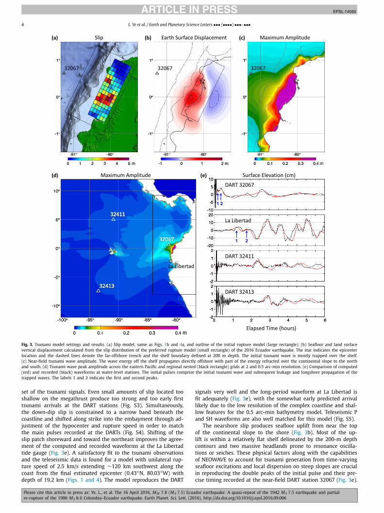
Fig. 3. Tsunami model settings and results. (a) Slip model, same as Figs. 1b and 4a, and outline of the initial rupture model (large rectangle). (b) Seafloor and land surface vertical displacement calculated from the slip distribution of the preferred rupture model (small rectangle) of the 2016 Ecuador earthquake. The star indicates the epicenter location and the dashed lines denote the far-offshore trench and the shelf boundary defined at 200 m depth. The initial tsunami wave is mostly trapped over the shelf. (c) Near-field tsunami wave amplitude. The wave energy off the shelf propagates directly offshore with part of the energy refracted over the continental slope to the north and south. (d) Tsunami wave peak amplitude across the eastern Pacific and regional nested (black rectangle) grids at 2 and 0.5 arc-min resolution. (e) Comparison of computed (red) and recorded (black) waveforms at water-level stations. The initial pulses comprise the initial tsunami wave and subsequent leakage and longshore propagation of the trapped waves. The labels 1 and 2 indicate the first and second peaks.

set of the tsunami signals. Even small amounts of slip located too shallow on the megathrust produce too strong and too early first tsunami arrivals at the DART stations (Fig. S3). Simultaneously, the down-dip slip is constrained to a narrow band beneath the coastline and shifted along strike into the embayment through ad-justment of the hypocenter and rupture speed in order to match the main pulses recorded at the DARTs (Fig. S4). Shifting of the slip patch shoreward and toward the northeast improves the agree-ment of the computed and recorded waveforms at the La Libertad tide gauge (Fig. 3e). A satisfactory fit to the tsunami observations and the teleseismic data is found for a model with unilateral rup-ture speed of 2.5 km/s extending ∼120 km southwest along the coast from the final estimated epicenter (0.43◦N, 80.03◦W) with depth of 19.2 km (Figs. 1 and 4). The model reproduces the DART

signals very well and the long-period waveform at La Libertad is fit adequately (Fig. 3e), with the somewhat early predicted arrival likely due to the low resolution of the complex coastline and shal-low features for the 0.5 arc-min bathymetry model. Teleseismic P and SH waveforms are also well matched for this model (Fig. S5).

The nearshore slip produces seafloor uplift from near the top of the continental slope to the shore (Fig. 3b). Most of the up-lift is within a relatively flat shelf delineated by the 200-m depth contours and two massive headlands prone to resonance oscilla-tions or seiches. These physical factors along with the capabilities of NEOWAVE to account for tsunami generation from time-varying seafloor excitations and local dispersion on steep slopes are crucial in reproducing the double peaks of the initial pulse and their pre-cise timing recorded at the near-field DART station 32067 (Fig. 3e).

JID:EPSL AID:14050 /SCO [m5G; v1.189; Prn:30/09/2016; 14:04] P.5 (1-11)

L. Ye et al. / Earth and Planetary Science Letters ••• (••••) •••–••• 5

Fig. 4. The preferred finite-fault source model for the 2016 Ecuador earthquake iteratively constrained by teleseismic and tsunami waves modeling. The fault model has a strike φ = 5◦ , variable dip angle shown in Fig. S2 and average rake λ = 126.4◦ , with a rupture expansion speed of 2.5 km/s. (a) The moment rate function (MRF) for the slip model. (b) Far-field source spectrum, combining the MRF spectrum for frequencies <0.05 Hz, and logarithmically averaged P-wave displacement spectra corrected for radiation pattern, geometric spreading, and attenuation at 0.05 to 2.0 Hz. The dashed curve shows a reference ω−2 spectrum with 3 MPa stress parameter. (c) Inverted slip distribution with slip vector and source time function in each subfault. Dashed lines indicate 10 s rupture isochrones. (d) The stress change at the mid-point of each subfault computed for the entire distribution of slip over the model surface. The stress drops calculated by trimming off those subfaults that have a seismic moment less than 15% of the peak subfault moment and using the remaining average slip and residual fault area, �σ0.15 is 2.0 MPa. The slip-weighted stress drop measured from the variable stress change distribution, �σE is 2.8 MPa. (e) P and SH radiation patterns and lower hemisphere data sampling for waveforms used in the inversion and the average focal mechanism. Animation of the slip history is presented in Supporting Information Movie M4.

The first peak is overlapped by the tail end of the ground surface wave motion, but its longer duration in comparison to the ground motion pulse width points to the source being from an ocean sur-face wave. This is corroborated by the double-peaked feature in the initial arrivals at DARTs 32411 and 32413, which are far away from the seismic source. Animation M2 in the Supporting Infor-mation shows that the first peak at DART 32067 and La Libertad originates from the initial sea surface uplift over the continental slope that propagates directly offshore with part of the energy re-fracted along the continental slopes to the north and south. The initial pulse over the shelf is trapped as partial standing waves and subsequent energy leakage accounts for the second peak at DART 32067 with a small lag associated with the shelf processes.

The continental shelf functions like a waveguide channeling tsunami waves along its length through internal reflection, when

the propagation speed varies rapidly across the steep continental slope. The presence of canyons and headlands reflect the long-shore edge waves effectively trapping the energy along the shelf. This explains the persistent oscillations with considerable am-plitude at the La Libertad tide gauge after the first two small peaks from the initial tsunami pulse (Fig. 3e). The shelf environ-ment is conducive to belated arrivals of the peak wave during a tsunami event (Cheung et al., 2013; Yamazaki and Cheung, 2011;Yamazaki et al., 2013). Animation M3 illustrates the propagation of the tsunami across the ocean and the formation of the initial pulse at DART 32411 and 32413 from the initial sea surface up-lift on the continental slope and the subsequent energy release from inside the shelf. The recorded tsunami waveforms, which are highly sensitive to the location of the initial tsunami pulse in re-lation to the continental slope and shelf, allow precise placement

JID:EPSL AID:14050 /SCO [m5G; v1.189; Prn:30/09/2016; 14:04] P.6 (1-11)

6 L. Ye et al. / Earth and Planetary Science Letters ••• (••••) •••–•••

Fig. 5. (a) Comparison of the preferred slip model with distribution of coherent high-frequency seismic radiation derived from back-projection of teleseismic body-waves filtered between 0.5 and 2 Hz. Stars and diamonds indicate the locations of bursts of high-frequency seismic radiation from teleseismic P waves recorded of NA and EU networks, respectively. These are color-coded by the elapsed time from the origin, and indicate a rupture speed of ∼2 to 3 km/s. (b) Location of aftershocks over 35 days following the mainshock from the Geophysical Institute of the National Polytechnic School at Ecuador (http :/ /www.igepn .edu .ec /portal /ultimo-sismo /informe-ultimo-sismo .html) superimposed on the slip model.

of the near-shore slip in this case. It also strongly rules out slip further seaward under the continental slope or near the trench.

It is well known that finite source models can be significantly improved, in particular regarding the absolute and details of the main slip patches, when geodetic or remote sensing data are in-cluded in the inversion (e.g., Konca et al., 2008). As the discus-sion above shows, the tsunami data provide similar constraints on the offshore part of the source model. Onshore measurement of ground displacements would be helpful to constrain further the down-dip part of the slip distribution. In the absence of avail-able geodetic ground deformation data, we have compared the predictions of our final slip model with line-of-sight (LOS) dis-placement maps derived from SAR interferometry using Sentinel-1A and ALOS-2 satellites (Xu and Sandwell, personal communica-tion, 2016; Spaans and Hooper, personal communication, 2016). As these results are preliminary and not yet published, we used them only for reality check. We find that our model (see model predic-tions in Fig. S6) is very consistent to first order with the location, pattern and amplitude of the ground displacement measured from these SAR images. We note in particular that the minor slip patch at the southeast corner of the source, which explains the tail of the moment rate distribution, between 60 s and 75 s, helps re-produce the SAR observations. Minor discrepancies are observed though. They suggest that the down-dip extent of our slip distri-bution may extend a bit too far to the east. While there is no doubt that the inclusion of SAR and GPS data will help refine the source model, we anticipate that only minor modifications of our best fit-ting model will be necessary.

Our final slip model (Fig. 4) shows a patch of large slip near the hypocenter with a larger separate patch extending from 30 to 100 km southward from the hypocenter, consistent with the back-projection images (Fig. 5a). The space–time slip history is shown in Animation M4. The peak slip is ∼5 m, and the average slip, after removing those subfaults with inverted seismic moment less than 15% of the peak subfault seismic moment, is ∼2.0 m. The slip-weighted static stress drop is ∼2.8 MPa (Ye et al., 2016a), a value

typical of ordinary interplate earthquakes. The radiated energy, up to ∼1 Hz, for the 2016 event estimated from teleseismic data with the method of Ye et al. (2016a) is 4.60 × 1015 J (Fig. 4). The cor-responding moment-scaled radiated energy is 8.5 × 10−6 and the radiation efficiency is ∼0.21, similar to the average values for large megathrust earthquakes.

3. Historical earthquakes: 1906, 1942, 1958 and 1979

The slip distribution for the 2016 Ecuador earthquake encom-passes the hypocenter and likely source region inferred from after-shocks for the 1942 earthquake (Fig. 1). To further assess whether these events are comparable, we evaluated historical measure-ments and seismic recordings for the 1942 event, and the other large events along the coast in 1906, 1958, and 1979.

One of the key measures of the size of historic large events is provided by surface wave magnitude, but comparisons have to be made carefully due to changes in measurement procedures over time. Although various values are cited in the literature for the 1906, 1942, and 1958 events, we primarily use the data listed in Beno Gutenberg’s notepads (Goodstein et al., 1980), which are the basis of Gutenberg and Richter (1954). For the 1979 and 2016 events, we use the data provided by USGS-NEIC. We also use Abe’s (1981) catalog for cross checking. Although the M S values listed in these catalogs vary in minor details, they are generally consis-tent (e.g., Abe, 1981; Lienkaemper, 1984) and are appropriate for the purpose of this study. Fig. 6 compares the M S values for the 1979 and 2016 events listed by USGS-NEIC, along with those for earlier events taken primarily from the Gutenberg Notepads (see Table S3 for details). USGS-NEIC lists the average M S of the 1979 and the 2016 events as 7.7 and 7.5, respectively. Abe (1981) gives M S = 7.6 for the 1979 event. As indicated by the data for the 1979 and 2016 events, the scatter of the M S values between stations is very large, ranging over 1.5 magnitude units. This amount of scatter is common and is most likely a result of complex multi-pathing and interference of surface waves. Thus, a straight average

JID:EPSL AID:14050 /SCO [m5G; v1.189; Prn:30/09/2016; 14:04] P.7 (1-11)

L. Ye et al. / Earth and Planetary Science Letters ••• (••••) •••–••• 7

Fig. 6. Surface wave MS measurements for 1906, 1942 and 1958 earthquakes (mainly from Gutenberg’s notepads with a few points from station bulletins and seismic records), and MS for the 1979 and 2016 events from USGS/PDE (see detailed information in Table S3).

or median of the measured values can be misleading, especially when the azimuthal coverage is limited as is the case for most old events. This large scatter suggests that even if individual measure-ments are correct, the uncertainty in the average M S for old events appears to be at least 1/4 M S unit. In some cases, it can be even larger, and we must keep in mind this amount of uncertainty in in-terpreting the M S for old events. Although Gutenberg and Richter(1954) assign M S(G-R) = 7.9 to the 1942 event, Fig. 6 shows that the station M S values for the 1942 event taken from the Gutenberg notepad (red stars) follow approximately the same azimuthal trend with rather high values as the better sampled 2016 event, suggest-ing that the average M S of the 1942 event is approximately the same as that of the 2016 event, i.e., M S = 7.5. The M S values at in-dividual stations for the 1958 event are close to, or slightly below, the trend of the 2016 event. Thus, M S = 7.3 given by Abe (1981)appears reasonable. In contrast, the station M S values for the 1906 event are consistently larger than those for the other events. In fact, Gutenberg and Richter (1954) and Abe (1981) list this event as M S = 8.6 and 8.7, respectively. However, some catalogs (e.g., Abe and Noguchi, 1983) revised it to 8.2 primarily because they suspected that some amplitude data were obtained from the un-damped Milne records. However, the 1906 event’s M S values for stations like Potsdam, Leipzig, and Jena were probably from the damped Wiechert records. Also our own measurement from the Omori seismograms at Mizusawa gives M S = 8.5. Thus, we be-lieve that M S of the 1906 event is considerably larger than for the other events in this sequence, and the Gutenberg and Richter(1954) M S = 8.6 is reasonable. In this study, we adopt M S = 8.6, 7.5, 7.3, 7.7, and 7.5 for the 1906, 1942, 1958, 1979, and 2016 events, respectively. Given the uncertainties arising from unknown instrument calibration, insufficient azimuthal coverage, station cor-rections, and complex and yet not-fully-understood path effects, any difference smaller than 1/4 M S unit should not be given much significance.

In addition to M S , for a more quantitative understanding of the slip budget it is important to determine the seismic moment (i.e., MW ) estimated at very long period. For the 1979 and 2016 events, MW is relatively well constrained to 8.1 (gCMT) and 7.8 (gCMT and W-phase solutions), respectively. The moment of the 1958 event is estimated to be smaller than the 1979 event by 0.5 MW unit

(i.e. MW ∼ 7.6) (Kanamori and McNally, 1982). Swenson and Beck(1996) estimated M0 = 6 to 8 ×1020 N-m (MW ∼ 7.8) for the 1942 event, although this value appears somewhat uncertain because of the limited frequency band for the data used and uncertain instru-ment calibration. No reliable estimate of MW from seismic data is available for the 1906 event, despite being the largest event in the sequence.

Okal (1992) compared the Wiechert seismograms of the 1979 and 1906 event recorded at Uppsala (UPP). According to Kulhánek(1988), the response of the Uppsala Wiechert seismographs re-mained essentially constant. Thus, the comparison made by Okal(1992) is most relevant and important. The records for the 1906 and the 1979 events are taken from Okal (1992), and that for the 2016 event is taken from the GSN record at station KONO, here used as a proxy of the record at UPP. The Wiechert seismogram for KONO is simulated from the GSN broad-band record by deconvo-lution of the instrument response and convolution of the Wiechert response. The similarity in dispersion to that for the 2016 event, which has three component seismic data, confirms that the UPP signal for the 1906 event is the G1 Love wave. Fig. 7a shows com-parisons of 3 different period passbands, 100–500 s, 150–500 s, and 200–500 s. The increase in the peak-to-peak amplitude ra-tios with period probably reflects the corner frequency shift toward low frequency with increasing MW . However, given the extremely low gain at long period, the solid friction between the recording stylus and paper, and hand digitization error, the ratios for the 200–500 s passband are less reliable. We choose the ratios for the 150–500 s passband to estimate the MW differences. The ratios for the 150–500 s band are 1906/1979 = 2.9 and 1906/2016 = 17.8, corresponding to MW differences of 0.3 and 0.8, respectively. Also, the 1906 seismogram is larger by a factor of 1.35 than the syn-thetic seismogram computed for an MW = 8.5 event with the mechanism of the 2016 event, corresponding to �MW ∼ 0.1. Thus, these comparisons indicate that MW of the 1906 event is ∼8.6 which is comparable to the tsunami magnitude Mt (8.5 to 8.7) (Ta-ble S1).

The comparable M S and aftershock distributions (Figs. 1a and S7) of the 1942 and 2016 events suggest a similar rupture area. Fortunately, we have obtained P waves recorded for both 1942 and 2016 events for direct comparisons from seismic stations at

JID:EPSL AID:14050 /SCO [m5G; v1.189; Prn:30/09/2016; 14:04] P.8 (1-11)

8 L. Ye et al. / Earth and Planetary Science Letters ••• (••••) •••–•••

Fig. 7. (a) Comparison of N–S component G1 of the 1906 (red), 1979 and 2016 earthquakes. The data for 1906 and 1979 event are recorded by UPP Wiechert instrument with pendulum period ∼6.8 s, peak gain ∼230 and damping ε = 3 (modified from Okal, 1992). The waveform for the 2016 event is the convolution of displacement (after removal of the broadband instrumental response) at station KONO (close to UPP) and the Wiechert instrumental response. Comparisons of long-period signals at frequency bands of 100–500 s, 150–500 s and 200–500 s for 1906, 1979 and 2016 events, along with peak-to-peak amplitudes, are shown. The gray curves are synthetic seismogram with corresponding frequency bands from the 1906 hypocenter to the UPP site with MW 8.5, same focal mechanism of the 2016 event and PREM earth structure. (b) Comparisons of vertical P-wave waveforms at Pasadena (PAS) with 1–90 s Benioff instrumental response (peak gain of 3000 at period of 1 s) between 1942 (purple), 1958 (black), 1979 (green) and 2016 (blue) events. The corresponding peak-to-peak amplitudes are shown at the top of each panel. Waveforms for 1942, 1958, and 1979 events are digitized from Hartzell and Heaton (1985). Waveforms for the 1942 and 2016 event are aligned at the beginning (1st row) and at the peak (2nd row) for comparison. (c) Comparison of P waves at E–W component of the 1942 (purple) and 2016 (blue) events at station DBN with Galitzin instrumental response (pendulum/galvanometer periods ∼25 s and gain factor of 310). The waveform for 1942 is from Swenson and Beck (1996) with peak-to-peak amplitude confirmed by Bernad Dost from the DBN station bulletin. The waveform for the 2016 event is the convolution of displacement (after removal of the broadband instrumental response) with the Galitzin instrumental response. They are aligned at the beginning (left) and at the peak (right).

Pasadena, California (PAS) and at De Bilt, Netherlands (DBN) at dif-ferent azimuths. We simulate the waveforms for the 2016 event from the GSN broad-band records by deconvolution of the instru-ment response and convolution of the corresponding instrumental responses for the 1942 recording. The Benioff instrument at PAS is sensitive to signals with periods around 1 s to 90 s with peak gain at 1 s; and the Galitzin seismometer at DBN is sensitive to slightly longer periods with peak gain at 25 s. The recorded P waves at these two stations show substantial information about source complexity. Comparisons aligned with the initial and the peak at PAS and DBN are shown in Figs. 7b and 7c, respectively. The peak-to-peak amplitude ratios of 1942/2016 = 0.7 (PAS) and 1.25 (DBN) are close to 1, allowing for some uncertainties in in-strumental response, errors in reading historical paper data, and some variation in source. Discrepancy in duration from the on-set to the peak motion suggests some difference between the two ruptures, and the shorter signal interval for the 1942 event indi-cates that it may not have involved slip near the hypocenter of the 2016 event. The similar motions of the aligned waveforms with re-

spect to the peak between the two events show that the main slip area of the 2016 event probably overlaps that of the 1942 event. The intensity distributions (Fig. S8), even with strongly subjective and variable criteria, show very similar relative patterns between the two events. Altogether, based on these observations, the 2016 event appears to be a quasi-repeat of the 1942 event, with the main slip patch being in common. The short duration and low-amplitude P wave from the 1958 event at PAS is consistent with the small M S value. The P wave amplitude for the 1979 event is comparable to the 1942 and 2016 events, but the longer duration is consistent with its larger long-period magnitudes and stronger tsunami excitation (Kanamori and McNally, 1982; Beck and Ruff, 1984).

4. Discussion

The ∼2.0 m average slip for the 2016 MW 7.8 Ecuador earth-quake is commensurate with accumulated slip deficit since the 1942 earthquake given the patchy pattern of interseismic cou-

JID:EPSL AID:14050 /SCO [m5G; v1.189; Prn:30/09/2016; 14:04] P.9 (1-11)

L. Ye et al. / Earth and Planetary Science Letters ••• (••••) •••–••• 9

pling. It is equivalent to an average interseismic coupling ∼0.6 across the region given the 4.6 cm/yr convergence rate, which seems reasonable in view on the interseismic model of Chlieh et al. (2014) (Fig. 1a) and consistent with ∼50% locking on average from Trenkamp et al. (2002) and White et al. (2003). Our preferred slip model for the 2016 event shows two main large-slip patches with high static shear stress drop (>5 MPa). A minor deep asper-ity (at depth of ∼30 km) is inferred at the southeastern end of our model and relates to tapering of the rupture indicated by the tail of the moment rate function. This is in the vicinity of the MW 7.21998 and MW 7.0 1992 earthquakes. We infer rupture of several asperities beneath the coastline, a pattern also qualitatively con-sistent with the patchy interseismic locking pattern and location of the large slip deficit patches. A quantitative correlation analysis between the co-seismic slip distribution and interseismic coupling is not justified given the uncertainties of both quantities.

Aftershocks of the 2016 event from a regional catalog (Geo-physical Institute of the National Polytechnic School at Ecuador) cluster along streaks normal to the trench at the northern edge of the mainshock rupture at ∼0.8◦N and oblique to the trench along the equator (Figs. 5b and S7). Interestingly these clusters line up with the two main slip patches (Fig. 5b) extending up-dip of their shallow edges. The precise location of aftershocks is uncertain due to effects of uncertain velocity structure, station distribution, etc. However, the relative locations between aftershock are gen-erally more reliable and the same general patterns are evident in the smaller number of aftershocks determined by the USGS-NEIC. A possible interpretation is that the 2016 Ecuador earthquake trig-gered up-dip afterslip producing aftershocks, as was observed fol-lowing some large megathrust events such as the 2005 MW 8.6and 2007 MW 8.4 earthquakes offshore Sumatra (Hsu et al., 2006;Avouac, 2015).

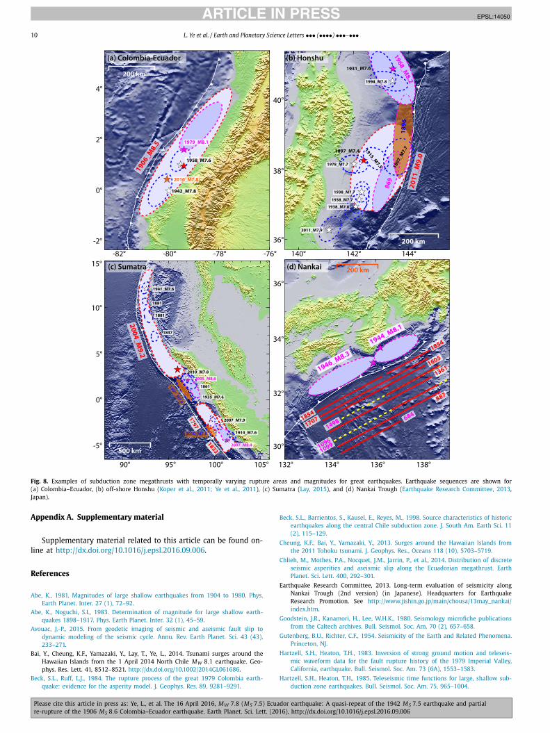
The 1906/1942–1958–1979–1998/2016 Ecuador–Colombia se-quence demonstrates substantial variability among successive rup-tures of the same subduction zone area. As pointed out by Kanamori and McNally (1982), the entire area can rupture in a great MW > 8.5 event or rupture piecewise in smaller events. Similar behavior has been observed elsewhere, for example, in Japan and Sumatra (e.g., Lay et al., 1982; Thatcher, 1990;Konca et al., 2008) (Fig. 8). An interesting aspect of the Ecuador–Colombia example is the similarity of the 1942 and 2016 events. Together with the observed patchy interseismic coupling pattern, this observation suggests that the seismic asperities are probably associated with persistent spatial variations of frictional properties of the megathrust over successive ruptures. The 2016 and 1942 events seem to have ruptured a similar subset of asperities, which probably also ruptured as part of the 1906 event (Fig. 8). Mechan-ical interactions and triggering between the adjacent slip patches are likely among the important causes for the non-characteristic behavior; temporal changes in the plate boundary frictional prop-erties can be another factor. Kaneko et al. (2010) numerically show that asperities, corresponding to area with rate-weakening friction interlaced in rate-strengthening areas, could produce such variable rupture scenarios as well as the repetition of similar events.

Spatial variations of frictional properties of the plate interface in the rupture area of the 1906 to 2016 earthquake sequence might be related to the influence of the Carnegie ridge, which is being subducted beneath the coast of Ecuador (Fig. 1). The subduction of a seismic ridge can lead to a complex pattern with seismic as-perities intermingled with aseismic creep areas as observed where the Nazca ridge is subducting beneath southern Peru (Perfettini et al., 2010); or where the Investigator fracture ridge is subducting beneath Sumatra (Konca et al., 2008).

Our estimate of MW (8.6) for the 1906 event based on wave-form comparisons is 0.2 magnitude units smaller than that of Kanamori and McNally (1982) based on aftershock zone area. The

moment of the 1906 event is still greater than the sum of the mo-ments for 1942, 1958, and 1979 events by a factor of three (rather than five). This may be because the asperities and surrounding ar-eas are driven to slip more during synchronized failure of multiple asperities than when ruptured in isolation. Given this variability, the ‘characteristic earthquake’ model (Schwartz and Coppersmith, 1984) for long-term hazard estimation is over-simplified. Rupture variability as observed for the Colombia–Ecuador sequence needs to be factored in when constructing scenario earthquake mod-els, as is done in the recent scenario earthquake project for the Nankai trough earthquake, Japan, where the historical data clearly demonstrate significant variability (Earthquake Research Commit-tee, 2013, Japan; Fig. 8d).

5. Conclusion

The benefit of jointly modeling teleseismic and tsunami obser-vations to constrain the location of coseismic slip during a large megathrust rupture is dramatically demonstrated by our model-ing for the 2016 Ecuador earthquake. The complex rupture pattern observed during the MW 7.8 2016 Ecuador earthquake suggests that it ruptured a common main asperity that had previously rup-tured in a similar event in 1942, and as part of a larger, M S 8.6event in 1906. The pattern of asperities ruptured in 2016 is con-sistent with the heterogeneous pattern of interseismic locking of the plate interface. Altogether these observations suggest that as-perities can be persistent features determined by the spatial vari-ations of the mechanical properties of the subduction megathrust. However, non-characteristic behavior due to synchronization and dynamic triggering lead to variable rupture dimensions and re-peat times as found for the 1906, 1942–1958–1979–1998, 2016 Ecuador–Colombia sequence. This is commonly observed. Detailed and quantitative studies of the rupture variability are needed to provide a basis for realistic scenario earthquake models.

Acknowledgements

The IRIS DMS data center (http :/ /www.iris .edu /hq/) was used to access the seismic data from Global Seismic Network and Fed-eration of Digital Seismic Network stations. Bernard Dost at the Royal Netherlands Meteorological Institute in Dutch helped check the peak-to-peak amplitude and the instrumental response for the 1942 event, and also provide the broadband record for the 2016 event at Debilt. Björn Lund at Uppsala university helped check the historical instrumental responses at Uppsala station. Omori seismograms for the 1906 earthquake are provided by the Mizu-sawa observatory. Stephen Hartzell and Tom Heaton provided high-resolution copies of Pasadena P waveforms records for the 1942, 1958 and 1979 events. The copies of the papers of the Gutenberg notepad are provided by the Archives of the California Institute of Technology. James Dewey at USGS provided us ISC-NEIC informa-tion on M S for 1979 and 2016 events. Stephen Hernandez helped provide access to the local seismic catalog. Mohamed Chlieh pro-vided his preferred geodetic coupling model. Yong Wei provided the post-processed DART and tide gauge time series, where the original data can be downloaded from the NOAA National Data Buoy Center (http :/ /www.ndbc .noaa .gov/) and CO-OPS Tsunami Capable Tide Stations (http :/ /tidesandcurrents .noaa .gov /tsunami/). David Sandwell and Xiaohui Xu at UC San Diego, Karsten Spaans and Andrew Hooper at Leeds showed us their InSAR images re-spectively for comparison, along with helpful discussions. This data analysis made use of GMT, SAC, and Matlab software. We thank Nadia Lapusta and Luis Rivera for helpful discussion. This work was supported by NSF grant EAR1245717 to Thorne Lay, and Caltech Seismological Laboratory Director’s fellowship to Lingling Ye.

JID:EPSL AID:14050 /SCO [m5G; v1.189; Prn:30/09/2016; 14:04] P.10 (1-11)

10 L. Ye et al. / Earth and Planetary Science Letters ••• (••••) •••–•••

Fig. 8. Examples of subduction zone megathrusts with temporally varying rupture areas and magnitudes for great earthquakes. Earthquake sequences are shown for (a) Colombia–Ecuador, (b) off-shore Honshu (Koper et al., 2011; Ye et al., 2011), (c) Sumatra (Lay, 2015), and (d) Nankai Trough (Earthquake Research Committee, 2013, Japan).

Appendix A. Supplementary material

Supplementary material related to this article can be found on-line at http://dx.doi.org/10.1016/j.epsl.2016.09.006.

References

Abe, K., 1981. Magnitudes of large shallow earthquakes from 1904 to 1980. Phys. Earth Planet. Inter. 27 (1), 72–92.

Abe, K., Noguchi, S.I., 1983. Determination of magnitude for large shallow earth-quakes 1898–1917. Phys. Earth Planet. Inter. 32 (1), 45–59.

Avouac, J.-P., 2015. From geodetic imaging of seismic and aseismic fault slip to dynamic modeling of the seismic cycle. Annu. Rev. Earth Planet. Sci. 43 (43), 233–271.

Bai, Y., Cheung, K.F., Yamazaki, Y., Lay, T., Ye, L., 2014. Tsunami surges around the Hawaiian Islands from the 1 April 2014 North Chile MW 8.1 earthquake. Geo-phys. Res. Lett. 41, 8512–8521. http://dx.doi.org/10.1002/2014GL061686.

Beck, S.L., Ruff, L.J., 1984. The rupture process of the great 1979 Colombia earth-quake: evidence for the asperity model. J. Geophys. Res. 89, 9281–9291.

Beck, S.L., Barrientos, S., Kausel, E., Reyes, M., 1998. Source characteristics of historic earthquakes along the central Chile subduction zone. J. South Am. Earth Sci. 11 (2), 115–129.

Cheung, K.F., Bai, Y., Yamazaki, Y., 2013. Surges around the Hawaiian Islands from the 2011 Tohoku tsunami. J. Geophys. Res., Oceans 118 (10), 5703–5719.

Chlieh, M., Mothes, P.A., Nocquet, J.M., Jarrin, P., et al., 2014. Distribution of discrete seismic asperities and aseismic slip along the Ecuadorian megathrust. Earth Planet. Sci. Lett. 400, 292–301.

Earthquake Research Committee, 2013. Long-term evaluation of seismicity along Nankai Trough (2nd version) (in Japanese). Headquarters for Earthquake Research Promotion. See http://www.jishin.go.jp/main/chousa/13may_nankai/index.htm.

Goodstein, J.R., Kanamori, H., Lee, W.H.K., 1980. Seismology microfiche publications from the Caltech archives. Bull. Seismol. Soc. Am. 70 (2), 657–658.

Gutenberg, B.U., Richter, C.F., 1954. Seismicity of the Earth and Related Phenomena. Princeton, NJ.

Hartzell, S.H., Heaton, T.H., 1983. Inversion of strong ground motion and teleseis-mic waveform data for the fault rupture history of the 1979 Imperial Valley, California, earthquake. Bull. Seismol. Soc. Am. 73 (6A), 1553–1583.

Hartzell, S.H., Heaton, T.H., 1985. Teleseismic time functions for large, shallow sub-duction zone earthquakes. Bull. Seismol. Soc. Am. 75, 965–1004.

JID:EPSL AID:14050 /SCO [m5G; v1.189; Prn:30/09/2016; 14:04] P.11 (1-11)

L. Ye et al. / Earth and Planetary Science Letters ••• (••••) •••–••• 11

Hayes, G.P., Wald, D.J., Johnson, R.L., 2012. Slab 1.0: a three-dimensional model of global subduction zone geometries. J. Geophys. Res. 117, B01302.

Hsu, Y.J., Simons, M., Avouac, J.P., Galetzka, J., Sieh, K., Chlieh, M., Natawidjaja, D., Prawirodirdjo, L., Bock, Y., 2006. Frictional afterslip following the 2005 Nias–Simeulue earthquake, Sumatra. Science 312 (5782), 1921–1926.

Kanamori, H., McNally, K.C., 1982. Variable rupture mode of the subduction zone along the Ecuador–Colombia coast. Bull. Seismol. Soc. Am. 72 (4), 1241–1253.

Kanamori, H., Rivera, L., 2008. Source inversion of W phase: speeding up seis-mic tsunami warning. Geophys. J. Int. 175, 222–238. http://dx.doi.org/10.1111/j.1365-246X.2008.03887.x.

Kaneko, Y., Avouac, J.P., Lapusta, N., 2010. Towards inferring earthquake patterns from geodetic observations of interseismic coupling. Nat. Geosci. 3 (5), 363–369.

Kelleher, J.A., 1972. Rupture zones of large South American earthquakes and some predictions. J. Geophys. Res. 77 (11), 2087–2103.

Kikuchi, M., Kanamori, H., 1982. Inversion of complex body waves—III. Bull. Seismol. Soc. Am. 81 (6), 2335–2350.

Konca, A.O., Avouac, J.P., Sladen, A., et al., 2008. Partial rupture of a locked patch of the Sumatra megathrust during the 2007 earthquake sequence. Nature 456 (7222), 631–635.

Koper, K.D., Hutko, A.R., Lay, T., Ammon, C.J., Kanamori, H., 2011. Frequency-dependent rupture process of the 2011 Mw 9.0 Tohoku Earthquake: comparison of short-period P wave backprojection images and broadband seismic rupture models. Earth Planets Space 63 (7).

Kulhánek, O., 1988. The status, importance and use of historical seismograms in Sweden. In: Historical Seismograms and Earthquakes of the World. Academic Press, San Diego, CA, USA, pp. 64–69.

Lay, T., 2015. The surge of great earthquakes from 2004 to 2014. Earth Planet. Sci. Lett. 409, 133–146.

Lay, T., Kanamori, H., Ruff, L., 1982. The asperity model and the nature of large subduction zone earthquake occurrence. EPR, Earthqu. Predict. Res. 1, 3–71.

Lay, T., Ye, L., Kanamori, H., Yamazaki, Y., et al., 2013. The February 6, 2013 Mw 8.0Santa Cruz Islands earthquake and tsunami. Tectonophysics 608, 1109–1121.

Li, L., Lay, T., Cheung, K.F., Ye, L., 2016. Joint modeling of teleseismic and tsunami wave observations to constrain the 16 September 2015 Illapel, Chile, MW 8.3earthquake rupture process. Geophys. Res. Lett. 43. http://dx.doi.org/10.1002/2016GL068674.

Lienkaemper, J.J., 1984. Comparison of two surface-wave magnitude scales: M of Gutenberg and Richter (1954) and Ms of “Preliminary Determination of Epicen-ters”. Bull. Seismol. Soc. Am. 74 (6), 2357–2378.

Megard, F., 1987. Cordilleran Andes and Marginal Andes: a review of andean geol-ogy North of Arica elbow (18′′). In: Monger, J.W.H., Francheteau (Eds.), Circum-Pacific Orogenic Belts and Evolution of the Pacific Ocean Basin. In: J. Geodyn. Ser., vol. 18. Am. Geophys. Union, Washington, DC.

Mendoza, C., Dewey, J.W., 1984. Seismicity associated with the great Colombia–Ecuador earthquakes of 1942, 1958 and 1979: implications for barrier models of earthquake rupture. Bull. Seismol. Soc. Am. 74 (2), 577–593.

Nishenko, S.P., 1991. Circum-Pacific seismic potential: 1989–1999. Pure Appl. Geo-phys. 135, 169–259.

Nocquet, J.M., Villegas-Lanza, J.C., Chlieh, M., et al., 2014. Motion of continental sliv-ers and creeping subduction in the northern Andes. Nat. Geosci. 7, 287–291.

Okada, Y., 1985. Surface deformation due to shear and tensile faults in a half space. Bull. Seismol. Soc. Am. 75 (4), 1135–1154.

Okal, E.A., 1992. Use of the mantle magnitude Mm for the reassessment of the mo-ment of historical earthquakes. Pure Appl. Geophys. 139 (1), 17–57.

Perfettini, H., Avouac, J.P., Tavera, H., et al., 2010. Seismic and aseismic slip on the Central Peru megathrust. Nature 465 (7294), 78–81.

Schwartz, D.P., Coppersmith, K.J., 1984. Fault behavior and characteristic earth-quakes: examples from the Wasatch and San Andreas fault zones. J. Geophys. Res. 89, 5681–5698.

Swenson, J.L., Beck, S.L., 1996. Historical 1942 Ecuador and 1942 Peru subduction earthquakes, and earthquake cycles along Colombia–Ecuador and Peru subduc-tion segments. Pure Appl. Geophys. 146 (1), 67–101.

Tanioka, Y., Satake, K., 1996. Tsunami generation by horizontal displacement of ocean bottom. Geophys. Res. Lett. 23, 861–864.

Thatcher, W., 1990. Order and diversity in the modes of Circum-Pacific earthquake recurrence. J. Geophys. Res. 95 (B3), 2609–2623.

Trenkamp, R., Kellogg, J.N., Freymueller, J.T., Mora, H.P., 2002. Wide plate margin deformation, southern Central America and northwestern South America, CASA GPS observations. J. South Am. Earth Sci. 15 (2), 157–171.

White, S.M., Trenkamp, R., Kellogg, J.N., 2003. Recent crustal deformation and the earthquake cycle along the Ecuador–Colombia subduction zone. Earth Planet. Sci. Lett. 216 (3), 231–242.

Xu, Y., Koper, K.D., Sufri, O., Zhu, L., Hutko, A.R., 2009. Rupture imaging of the MW 7.9 12 May 2008 Wenchuan earthquake from back projection of teleseismic P waves. Geochem. Geophys. Geosyst. 10, Q04006. http://dx.doi.org/10.1029/2008GC002335.

Yamazaki, Y., Cheung, K.F., 2011. Shelf resonance and impact of near-field tsunami generated by the 2010 Chile earthquake. Geophys. Res. Lett. 38, L12605. http://dx.doi.org/10.1029/2011GL047508.

Yamazaki, Y., Kowalik, Z., Cheung, K.F., 2009. Depth-integrated, non-hydrostatic model for wave breaking and run-up. Int. J. Numer. Methods Fluids 61 (5), 473–497.

Yamazaki, Y., Cheung, K.F., Kowalik, Z., 2011. Depth-integrated, non-hydrostatic model with grid nesting for tsunami generation, propagation, and run-up. Int. J. Numer. Methods Fluids 67 (12), 2081–2107.

Yamazaki, Y., Cheung, K.F., Lay, T., 2013. Generation mechanism and near-field dy-namics of the 2011 Tohoku tsunami. Bull. Seismol. Soc. Am. 103, 1444–1455. http://dx.doi.org/10.1785/0120120103.

Ye, L., Lay, T., Kanamori, H., 2011. The Sanriku-Oki low-seismicity region on the northern margin of the great 2011 Tohoku-Oki earthquake rupture. J. Geophys. Res. 117, B02305. http://dx.doi.org/10.1029/2011JB008847.

Ye, L., Lay, T., Kanamori, H., Rivera, L., 2016a. Rupture characteristics of major and great (Mw ≥ 7) megathrust earthquakes from 1990–2015: 1. Moment scaling relationships. J. Geophys. Res. 121, 821–844.

Ye, L., Lay, T., Kanamori, H., Koper, K.D., 2016b. Rapidly estimated seismic source parameters for the 16 September 2015 Illapel, Chile Mw 8.3 earthquake. Pure Appl. Geophys. 173 (2), 321–332.