OCEAN/ESS 410 Fall 2006

1

Exercise 9. Earthquake Focal Mechanisms Due in class: Tuesday, November 14 In this class we are going to use P wave first motions to obtain a double-couple focal mechanism for a subduction zone earthquake. The exercise was developed by John Louie at the University of Nevada, Reno and much what follows is taken from his class web site at http://www.seismo.unr.edu/ftp/pub/louie/class/333/mechanism.html. The goal of this exercise is two-fold 1. To help you understand how earthquakes are analyzed to determine fault planes. 2. To develop your geometric understanding of beach-ball plots so that you can look at them and visualize the fault planes and fault motions. We will work with seismograms from a magnitude 4.7 earthquake that occurred in a subduction zone on the east side of the North Island of New Zealand. The exercise has 5 parts 1. Picking P-wave polarities 2. Determining the take of direction (azimuth and inclination) of the seismic rays to each station 3. Plotting the take-off directions and polarities with a stereonet 4. Fitting two focal planes (i.e., alternate fault planes) to the polarities with the stereonet 5. Interpreting the results. (Steps 3 and 4 may be quite difficult especially if you have never used a stereonet and while I have tried to write clear instructions, it will be easiest to learn in class) As discussed in class, the first motions of P waves radiated from the double-couple earthquake are compressional in two quadrants (half-hemispheres) and dilatational the other two. A P wave propagating out of a compressional quadrant will initially shift the ground upwards when it reaches a seismic recorder. For this exercise we will use recorders that have recorded ground motion in the vertical direction. Seismograms from such instruments will initially move up (positive polarity) when they are from a compressional quadrant. Seismograms from vertical instruments in a dilatational quadrant will move down (negative polarity). The polarity of seismogram motions after the first motion is extremely complicated. Seismometers that are on the nodal plane between the compressional and dilatational quadrants of an earthquake do not record a strong first motion. Instead of being impulsive, their first arrivals are emergent. These are called nodal seismograms. Part 1. First-motion polarities Figure 1 shows 13 seismograms recorded from a magnitude 4.7 aftershock of the Magnitude 6.2 May 1990 Weber II earthquake on the east side of the North Island of New Zealand. All the seismograms are from vertical instruments, located as indicated. Seismogram swings in the up direction have a positive polarity. Look for an initial rise (or fall) out of the pre-arrival noise that looks more like an exponential curve than a sine wave. Note how the vibrations recorded by more distant stations have lower frequency. Relative record time increases to the right; these

OCEAN/ESS 410 Fall 2006

2

seismograms only plot arrivals in a 3-second window with the first motion about one second from the left side. Circle the first motion on each one (do not obscure the wiggles with your pen). Identify whether each first motion is compressional, dilatational, or nodal, and write your identification to the right of each seismogram and in the Table at the end of this exercise. Part 2. Ray take-off directions Because seismic velocities generally change with depth (and often with horizontal position), it is generally necessary to use a computer code that calculates ray path that obey Snell’s Law. However, for this earthquake the rays can be approximated as straight lines between the earthquake and the seismic stations Figure 2 shows a map of the stations and the earthquake. (a) Use a protractor to measure the azimuth between the earthquake epicenter and the seismic stations and record it in the Table at the end of this exercise. The azimuth is measured in degrees clockwise from North (it can vary between 0° and 360°). (b) Calculate a scale from the map and use this to measure the horizontal distances in kilometers between the earthquake epicenter and the seismic stations. Record these in the table. (c) To get a ray’s inclination (Θ in the figure below), use the horizontal distance you have measured from the earthquake's epicenter to the recording station, and the earthquake's 16.7 km depth. The depth divided by the distance is the tangent of the inclination. Take the inverse tangent (arctangent) of this quantity to get the inclinations. Record these in the table.

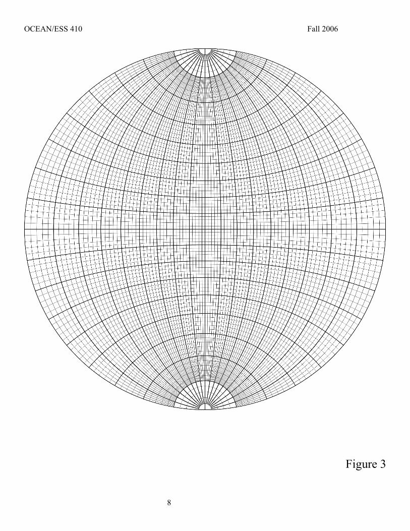
Part 3. Plotting polarities on the focal sphere The next step is to use a stereonet to plot the takeoff directions. When we plot the take off directions as points that mark the intersection of the ray with a sphere with the earthquake at its center. The Wolff stereographic projection provides a means to project points on the surface of a sphere onto a disk and to project the great circle lines that are formed by any plane that divides the sphere into two hemispheres. The stereonet is attached as Figure 3 to this exercise.

OCEAN/ESS 410 Fall 2006

3

The stereonet grid has a spacing of 2°. Points that plot around the rim of the stereonet represent horizontal take off directions (Θ = 0°) with the azimuth as shown. As one moves towards the center of the stereonet, the take-off inclination increases until it is vertical at the center point (Θ=90°). The line that extends from the center point to the Northern edge of the stereonet can be used to measure inclinations. To setup your Stereonet, do the following i. Insert a drawing pin pointing upwards through the center of the stereonet ii. Place a piece of tracing paper on top so it can rotate about the pin iii. In pencil, trace around the outer circle and mark north with a tick and the letter ‘N’ To plot your take off directions on the Stereonet do the following for each station iv. Rotate the tracing paper anticlockwise by the take-off azimuth (i.e., for an azimuth of 135° rotate the tracing paper 135° anticlockwise so that the north tick aligns with 225° on the underlying stereonet) v. Measure off the inclination downwards along the northern axis of the stereonet. vi. In pencil, plot a small filled circle for a compressional arrival, a small open circle for a dilatational arrival, and an ‘X’ for a nodal arrival. Number each arrival on your plot in case you need to come back and revise any of the polarities. Part 4. Fitting a focal mechanism to the polarities This is the hardest part of the exercise. The goal is to draw two orthogonal planes that represent the alternative fault planes that separate the first motions into compressional and dilatational quadrants. This is likely to involve quite a lot of trial and error and you may have to go back and revise some of your polarity determinations from Part 1. Draw your focal planes with a feint pencil so they can easily be erased until they are finalized. The Wulff stereonet includes lines of longitude connecting the north and south poles - these represent the projections of planes dipping at various angles. To draw two orthogonal planes do the following (i) Rotate the tracing paper to the desired orientation and trace over the desired ‘line of longitude’ to get the first plane (ii) Before rotating the tracing paper mark a ‘+’ at a point that is 90 degrees away from the plane you have just drawn by counting 90° horizontally on the paper away from the point that marks the intersection of the plane and the horizontal line that passes through the center point of the stereonet. (iii) Rotate the tracing paper to the desired orientation and trace over the “line of longitude” that passes through the ‘+’. This second plane will now be at orthogonal to the first. The trick is to draw the two planes so that they divide the compressional and dilatational quadrants. If you are lucky, all the compressional first motions will fall within the compressional quadrants, all the dilatational motions in the dilatational quadrants, and all the nodal rays within 10° of the fault or auxiliary plane. This rarely happens; you may have to look at the seismograms again and re-interpret a polarity or two. You may find that you cannot find any solution that fits all the polarities in which case you need to fit as many as you can.

OCEAN/ESS 410 Fall 2006

4

Part V. Interpretation To make your interpretation, it may help you to know that the Weber II earthquake sequence is above a shallow zone of westward subduction, that the subduction zone strikes northeast, and that the Weber II aftershocks align along a northwest-dipping plane (see figure below).

(a) What are the strikes and dips of the two focal planes (b) Draw a NW-SE cross-section through your solution showing the two possible orientations of the fault plane and the motions on each. Which is most compatible with the tectonics of the region. In this exercise we have been using an upper hemisphere projection (i.e., projecting rays that were taking off upwards on the stereonet). For large teleseismic earthquakes recorded by global seismic networks, the stations are 100’s and 1000’s of kilometers from the earthquake and the rays take off downwards. The focal mechanisms for teleseismic and regional earthquakes are usually plotted with a lower hemisphere projection.

(c) Sketch what your focal mechanism would look like using a lower hemisphere projection. Remember that the polarity at the opposite point on the sphere will always be the same. This is hard so if you get confused, talk to the instructor or TA.

OCEAN/ESS 410 Fall 2006

5

Table. Earthquake Data for Focal Mechanism Station Polarity (C, D,

or N) Azimuth, (° clockwise from N)

Horizontal Distance, km

Ray Inclination, Θ (° from horizontal)

1

2

3

4

5

6

7

8

9

10

11

12

13

Weber II Aftershock 127786, North Island, New Zealand 1990/05/1700:57 UTC Lon=176.3284° Lat=-40.2295° Depth=16.7 km Mag=4.73

-1 2Time, sec

Lon=176.35° Lat=-40.250° dist=3.4 km

Lon=176.17° Lat=-40.292° dist=14.4 km

Lon=176.37° Lat=-40.061° dist=19.1 km

Lon=176.28° Lat=-40.408° dist=20.2 km

Lon=176.06° Lat=-40.106° dist=25.9 km

Lon=176.47° Lat=-40.453° dist=28.0 km

Lon=176.63° Lat=-40.339° dist=29.1 km

Lon=176.09° Lat=-40.429° dist=29.9 km

Lon=176.27° Lat=-40.618° dist=43.5 km

Lon=176.81° Lat=-39.989° dist=49.0 km

Lon=176.35° Lat=-39.699° dist=59.0 km

Lon=176.88° Lat=-39.665° dist=78.4 km

Lon=176.82° Lat=-39.541° dist=87.5 km

1

2

3

4

5

6

7

8

9

10

11

12

13

Figure 1

175.8 176.0 176.2 176.4 176.6 176.8 177.0

-40.6

-40.4

-40.2

-40.0

-39.8

-39.6

Weber II Aftershock Records

Longitude

edutitaL

1

2

3

4

5

6

7

8

9

10

11 12

13

Figure 2

OCEAN/ESS 410 Fall 2006

8

Figure 3