PROCEEDINGS, 43rd Workshop on Geothermal Reservoir Engineering

Stanford University, Stanford, California, February 12-14, 2018

SGP-TR-213

1

Irregular Focal Mechanisms Observed at Salton Sea Geothermal Field: Possible Influences of

Anthropogenic Stress Perturbations

Aren Crandall-Bear1, Andrew J. Barbour1 and Martin Schoenball2

1 – United States Geological Survey, Menlo Park, CA, USA

2 – Lawrence Berkeley National Laboratory, Berkeley, CA, USA

acrandall-bear@usgs.gov, abarbour@usgs.gov, schoenball@lbl.gov

Keywords: Salton Sea Geothermal Field, fault reactivation, focal mechanisms, stress inversion, stress perturbation

ABSTRACT

At the Salton Sea Geothermal Field (SSGF), strain accumulation is released through seismic slip and aseismic deformation. Earthquake

activity at the SSGF often occurs in swarm-like clusters, some with clear migration patterns. We have identified an earthquake sequence

composed entirely of focal mechanisms representing an ambiguous style of faulting, where strikes are similar but deformation occurs

due to steeply-dipping normal faults with varied stress states. In order to more accurately determine the style of faulting for these events,

we revisit the original waveforms and refine estimates of P and S wave arrival times and displacement amplitudes. We calculate the

acceptable focal plane solutions using P-wave polarities and S/P amplitude ratios, and determine the preferred fault plane. Without

constraints on local variations in stress, found by inverting the full earthquake catalog, it is difficult to explain the occurrence of such

events using standard fault-mechanics and friction. Comparing these variations with the expected poroelastic effects from local

production and injection of geothermal fluids suggests that anthropogenic activity could affect the style of faulting.

1. INTRODUCTION

The southern Salton Sea is one of the most seismically active locations in southern California. Seismicity rates show an apparent

sensitivity to changes in the rates of injection and production of geothermal brine at the Salton Sea geothermal field (SSGF) (Llenos and

Michael, 2016), with an apparent insensitivity to dynamically triggered earthquakes (Zhang, et al., 2017). This suggests that the present-

day stress field at the SSGF has been altered from a more natural state by decades of net fluid production. Additionally, a subset of

earthquakes at the SSGF show an enigmatic faulting mechanism whereby dip-slip occurs on a near-vertical fault with very little oblique

slip. Although this style of faulting is at odds with classical fault-mechanics that assume a vertical-horizontal stress state, similar events

appear to be ubiquitous at seismically active geothermal fields in California (Schoenball, et al., 2016).

It is well known that at geothermal fields, injection and production of fluids are principal drivers of thermoelastic and poroelastic stress

changes (Segall and Fitzgerald, 1998) in addition to long-term pore pressure and temperature changes in the reservoir. In California

geothermal fields, stress changes in the reservoir manifest in geodetic data as a result of strain in the rock, for example, at Coso (Fialko

and Simons, 2000; Kaven, et al., 2017), The Geysers (Mossop and Segall, 1999; Vasco, et al., 2013), and Salton Sea (Barbour, et al.,

2016). While indirect links between poroelastic stress changes and aseismic deformation have been established at Salton Sea (Taira, et

al., 2018), it is not clear why this style of faulting is primarily observed at geothermal fields.

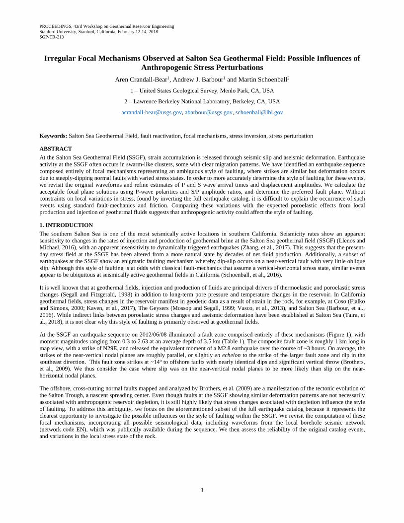
At the SSGF an earthquake sequence on 2012/06/08 illuminated a fault zone comprised entirely of these mechanisms (Figure 1), with

moment magnitudes ranging from 0.3 to 2.63 at an average depth of 3.5 km (Table 1). The composite fault zone is roughly 1 km long in

map view, with a strike of N29E, and released the equivalent moment of a M2.8 earthquake over the course of ~3 hours. On average, the

strikes of the near-vertical nodal planes are roughly parallel, or slightly en echelon to the strike of the larger fault zone and dip in the

southeast direction. This fault zone strikes at ~14o to offshore faults with nearly identical dips and significant vertical throw (Brothers,

et al., 2009). We thus consider the case where slip was on the near-vertical nodal planes to be more likely than slip on the near-

horizontal nodal planes.

The offshore, cross-cutting normal faults mapped and analyzed by Brothers, et al. (2009) are a manifestation of the tectonic evolution of

the Salton Trough, a nascent spreading center. Even though faults at the SSGF showing similar deformation patterns are not necessarily

associated with anthropogenic reservoir depletion, it is still highly likely that stress changes associated with depletion influence the style

of faulting. To address this ambiguity, we focus on the aforementioned subset of the full earthquake catalog because it represents the

clearest opportunity to investigate the possible influences on the style of faulting within the SSGF. We revisit the computation of these

focal mechanisms, incorporating all possible seismological data, including waveforms from the local borehole seismic network

(network code EN), which was publically available during the sequence. We then assess the reliability of the original catalog events,

and variations in the local stress state of the rock.

Crandall-Bear, Barbour, and Schoenball

2

Figure 1: Earthquakes and wells at the Salton Sea geothermal field. (A) Relocated earthquake locations (Yang, Hauksson,

Shearer, 2012) in grey, with events in the fault zone of interest highlighted. Elevations are from the 2010 USGS 1-meter

LiDAR-based digital elevation model; the tallest features are the volcanic buttes. Active geothermal wells are shown as

triangles for production, and inverted triangles for injection. (B) Seismicity colored by year of occurrence, in map view

(top) and isometric view (bottom), with well trajectories. (C) Monthly rates of geothermal fluid mass production,

injection, and net production, for the entire SSGF.

Table 1: Events in the composite fault zone

ID* Datetime M Longitude Latitude Depth

(UTC) (o East) (o North) (km)

15161057 2012-06-08 02:53:32 1.58 -115.6157 33.17683 3.56

15161097 2012-06-08 03:01:24 2.17 -115.6158 33.17617 3.53

15161153 2012-06-08 03:08:27 0.40 -115.6165 33.17533 3.59

15161193 2012-06-08 03:09:40 0.30 -115.6182 33.17300 3.65

15161225 2012-06-08 03:11:48 1.80 -115.6163 33.17583 3.64

15161241 2012-06-08 03:13:33 0.70 -115.6148 33.17767 3.49

15161297 2012-06-08 03:18:45 1.92 -115.6142 33.17916 3.48

15161345 2012-06-08 03:23:57 2.63 -115.6140 33.17883 3.32

15161425 2012-06-08 03:32:18 1.71 -115.6158 33.17633 3.58

15161537 2012-06-08 04:04:43 1.77 -115.6140 33.17867 3.32

15161585 2012-06-08 05:38:47 2.36 -115.6158 33.17667 3.53

15161993 2012-06-08 19:03:12 1.52 -115.6137 33.18067 3.38

* Focal mechanism id (and other data in table) from Yang, Hauksson, and Shearer (2012)

Crandall-Bear, Barbour, and Schoenball

3

2. METHODS

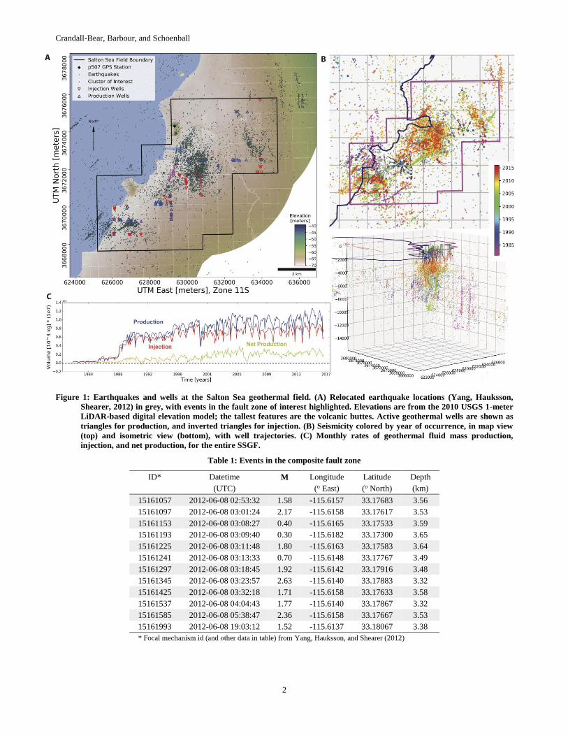
We first identify irregular focal mechanisms in the original YHS (Yang, Hauksson, and Shearer, 2012) focal mechanism catalog

following the classification system proposed by Frolich (1992), that uses the tensional and compressional directions, and the nodal plane

– the T, P, and B (or N) axes as they are commonly referred to. We impose an additional sub-classification (Figure 2) to exclude oblique

strike-slip mechanisms and further isolate pure, or very nearly pure dip-slip mechanisms. We then revisit the seismological data

associated with each event, downloading waveforms, phase picks and polarity data from the Southern California Earthquake Data

Center (SCEDC). Additionally, we downloaded data for the stations missing in the original analyses from the Incorporated Research

Institutions for Seismology Data Management Center (IRIS DMC), from both campaign and permanent seismic stations.

Figure 2: Ternary classification system, modified from Frolich (1992). The highlighted region represents the region we use to

identify events with pure dip slip on near-vertical planes.

Waveforms are integrated from counts to displacement using the available instrument response, and then bandpass filtered from 1 Hz up

to 90% of the Nyquist frequency, which varies owing to the diversity of seismic instrumentation. First motion polarities are identified,

and maximum amplitudes of the P and S-waves are calculated from the filtered, three-component records when pick information exists

in the SCEDC database. More specifically, P-wave amplitudes are calculated from the vector sum of the components, and S-wave

amplitudes calculated from the maximum displacement on any channel within 5 seconds of the apparent phase arrival (e.g., Hardebeck

and Shearer, 2003).

We reprocess the double-couple focal mechanism solutions with HASH (Hardebeck and Shearer, 2002, 2003) to determine the

acceptable and preferred mechanisms. For the HASH solutions we enforce a minimum of 8 polarities, a maximum azimuthal gap of 90

degrees, and 10% potential bad polarities in the solutions. Additionally, we specify 30 potential takeoff angles and azimuths for each

station, and 500 acceptable mechanisms allowed. We used the aggregate 1D velocity model included in the HASH program, which

includes a mixture of velocity models tailored for different regions (see Hardebeck and Shearer, 2002). These models do not account for

the three-dimensional velocity structure. Few tomographic images of the shallow structure of the SSGF exist, but McGuire, et al.,

(2015) show significant anomalies associated with the geothermal system. Although including either 3D velocity models or high-

resolution depth profiles from local borehole logging data would be useful to explore in future studies, doing so is well beyond the

scope of this project. We did, however, compare the HASH velocity models with the SCEC 3D Unified Velocity Model (i.e.,

Magistrale, et al., 2000) sampled at the SSGF, finding close agreement.

The new, best-fitting focal mechanisms are recombined with the original catalog, and then used to estimate variations in the local stress

field using SATSI (Hardebeck and Michael, 2006). The study area is discretized into 1 km by 1 km grid cells, and earthquake focal

mechanisms are associated with the nearest cell. Using the stress inversion results, we calculate the orientation of maximum horizontal

stress, 𝛼, at grid cells with well-resolved stress tensors following Lund and Townend (2007):

tan 2𝛼 =2[𝑙1𝑙2+(1−𝑅)𝑚1𝑚2]

(𝑙12−𝑙2

2)+(1−𝑅)(𝑚12−𝑚2

2), (1)

where l=(l1,l2,lz), m=(m1,m2,mz), and n=(n1,n2,nz), are the principal stress vectors associated with the respective principal stress

magnitudes, S1, S2, and S3 (S1 ≥ S2 ≥ S3); and

Crandall-Bear, Barbour, and Schoenball

4

1 − 𝑅 =𝑆2−𝑆3

𝑆1−𝑆3 (2)

3. RESULTS

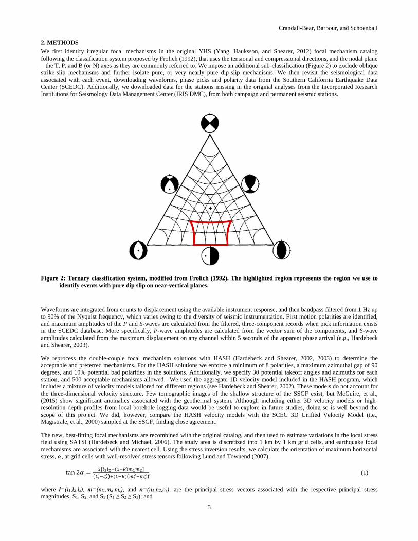
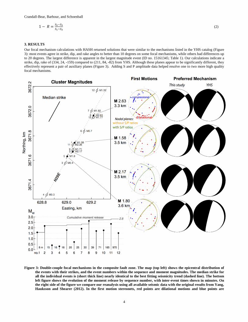
Our focal mechanism calculations with HASH returned solutions that were similar to the mechanisms listed in the YHS catalog (Figure

3): most events agree in strike, dip, and rake angles to better than 10 degrees on some focal mechanisms, while others had differences up

to 20 degrees. The largest difference is apparent in the largest magnitude event (ID no. 15161345; Table 1). Our calculations indicate a

strike, dip, rake of (334, 24, -159) compared to (211, 84, -82) from YHS. Although these planes appear to be significantly different, they

effectively represent a pair of auxiliary planes (Figure 3). Adding S and P amplitude data helped resolve one to two more high quality

focal mechanisms.

Figure 3: Double-couple focal mechanisms in the composite fault zone. The map (top left) shows the epicentral distribution of

the events with their strikes, and the event numbers within the sequence and moment magnitudes. The median strike for

all the individual events is (short thick line) nearly identical to the best fitting seismicity trend (dashed line). The bottom

left figure shows the evolution of the moment release by sequence number, with inter-event times shown in minutes. On

the right side of the figure we compare our reanalysis using all available seismic data with the original results from Yang,

Hauksson and Shearer (2012). In the first motion stereonets, red points are dilational motions and blue points are

Crandall-Bear, Barbour, and Schoenball

5

compressional motions; orange nodal planes represent results without S/P amplitude ratios, whereas green nodal planes

represent results including S/P amplitude ratios.

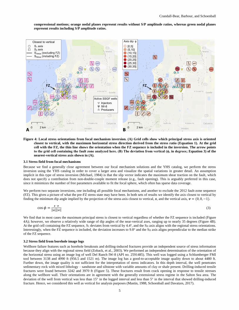
Figure 4: Local stress orientations from focal mechanism inversion. (A) Grid cells show which principal stress axis is oriented

closest to vertical, with the maximum horizontal stress direction derived from the stress ratio (Equation 1). At the grid

cell with the FZ, the thin line shows the orientation when the FZ sequence is included in the inversion. The arrow points

to the grid cell containing the fault zone analyzed here. (B) The deviation from vertical (ϕ, in degrees; Equation 3) of the

nearest-vertical stress axis shown in (A).

3.1 Stress field from focal mechanisms

Because we find a generally close agreement between our focal mechanism solutions and the YHS catalog, we perform the stress

inversion using the YHS catalog in order to cover a larger area and visualize the spatial variations in greater detail. An assumption

implicit in this type of stress inversion (Michael, 1984) is that the slip vector indicates the maximum shear traction on the fault, which

does not specify a contribution from non-double-couple moment release (e.g., fault opening). This is arguably preferred in this case,

since it minimizes the number of free parameters available to fit the focal sphere, which often has sparse data coverage.

We perform two separate inversions, one including all possible focal mechanisms, and another to exclude the 2012 fault-zone sequence

(FZ). This gives a picture of what the pre-FZ stress state may have been. In both sets of results we identify the axis closest to vertical by

finding the minimum dip angle implied by the projection of the stress axis closest to vertical, 𝒔, and the vertical axis, 𝒗 = (0, 0, −1).

cos 𝜙 =𝒔 ⋅ 𝒗

||𝒔||||𝒗|| (3)

We find that in most cases the maximum principal stress is closest to vertical regardless of whether the FZ sequence is included (Figure

4A); however, we observe a relatively wide range of dip angles of the near-vertical axes, ranging up to nearly 35 degrees (Figure 4B).

At the grid cell containing the FZ sequence, S1 deviates from vertical by 4.4o, and the SH axis aligns with the regional stress orientations.

Interestingly, when the FZ sequence is included, the deviation increases to 9.8o and the SH axis aligns perpendicular to the median strike

of the FZ sequence.

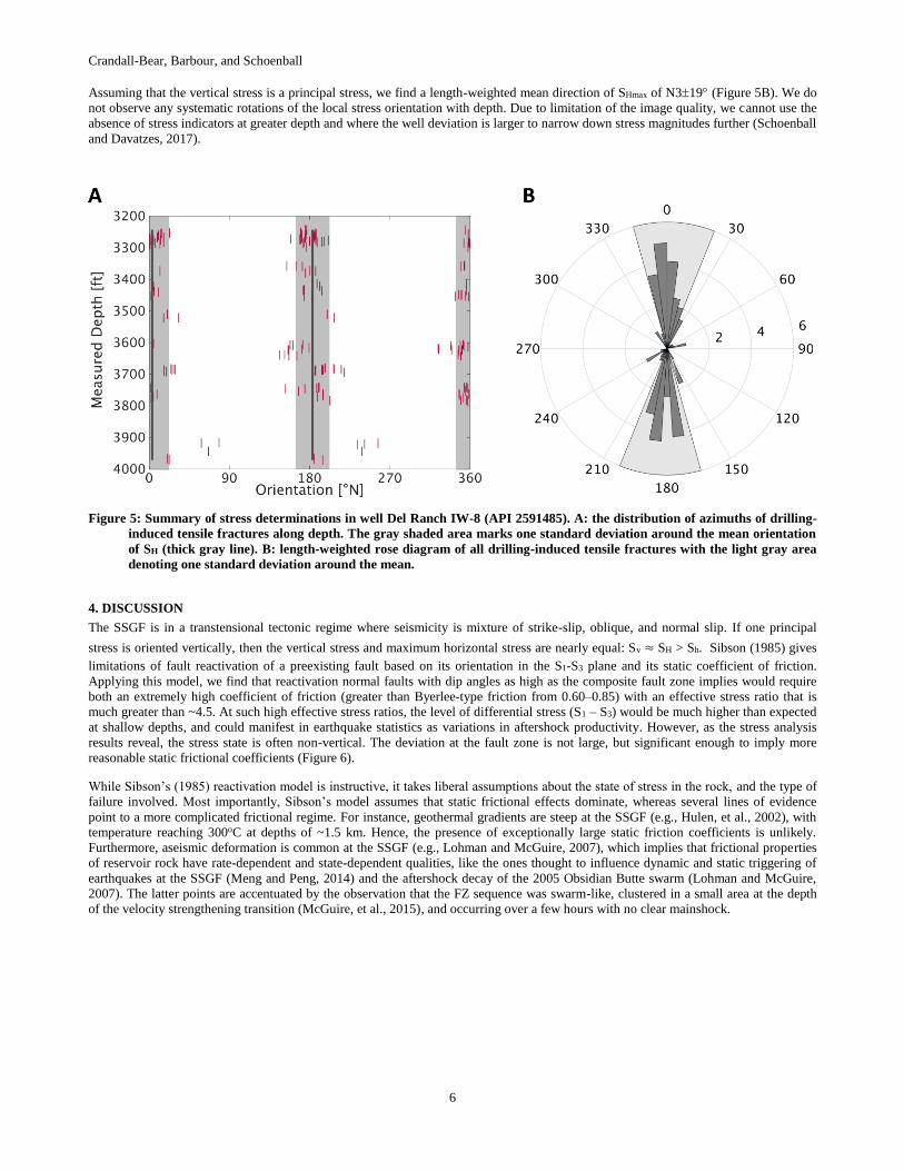
3.2 Stress field from borehole image logs

Wellbore failure features such as borehole breakouts and drilling-induced fractures provide an independent source of stress information

because they align with the regional stress field (Zoback, et al., 2003). We performed an independent determination of the orientation of

the horizontal stress using an image log of well Del Ranch IW-8 (API no. 2591485). This well was logged using a Schlumberger FMI

tool between 3138 and 4990 ft (956.5 and 1521 m). The image log has a good-to-acceptable image quality down to about 4480 ft.

Further down, the image quality is not sufficient for the interpretation of stress indicators. In this depth interval, the well penetrates

sedimentary rock with mixed lithology – sandstone and siltstone with variable amounts of clay or shale present. Drilling-induced tensile

fractures were found between 3242 and 3970 ft (Figure 5). These fractures result from crack opening in response to tensile stresses

along the wellbore wall. Their orientations are in agreement with the generally extensional stress regime in the Salton Sea area. The

deviation of the well from vertical was less than 15 in the logged interval and less than 5 in the interval that showed drilling-induced

fracture. Hence, we considered this well as vertical for analysis purposes (Mastin, 1988, Schoenball and Davatzes, 2017).

Crandall-Bear, Barbour, and Schoenball

6

Assuming that the vertical stress is a principal stress, we find a length-weighted mean direction of SHmax of N319 (Figure 5B). We do

not observe any systematic rotations of the local stress orientation with depth. Due to limitation of the image quality, we cannot use the

absence of stress indicators at greater depth and where the well deviation is larger to narrow down stress magnitudes further (Schoenball

and Davatzes, 2017).

Figure 5: Summary of stress determinations in well Del Ranch IW-8 (API 2591485). A: the distribution of azimuths of drilling-

induced tensile fractures along depth. The gray shaded area marks one standard deviation around the mean orientation

of SH (thick gray line). B: length-weighted rose diagram of all drilling-induced tensile fractures with the light gray area

denoting one standard deviation around the mean.

4. DISCUSSION

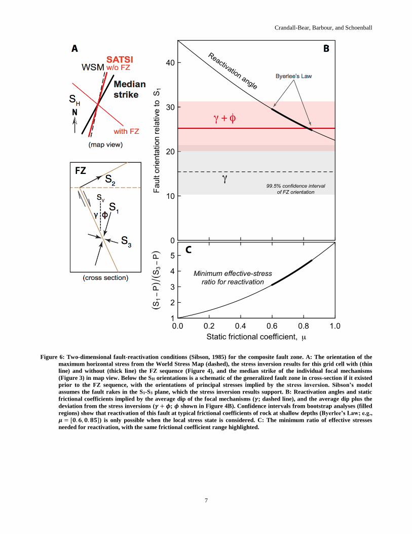
The SSGF is in a transtensional tectonic regime where seismicity is mixture of strike-slip, oblique, and normal slip. If one principal

stress is oriented vertically, then the vertical stress and maximum horizontal stress are nearly equal: Sv ≈ SH > Sh. Sibson (1985) gives

limitations of fault reactivation of a preexisting fault based on its orientation in the S1-S3 plane and its static coefficient of friction.

Applying this model, we find that reactivation normal faults with dip angles as high as the composite fault zone implies would require

both an extremely high coefficient of friction (greater than Byerlee-type friction from 0.60–0.85) with an effective stress ratio that is

much greater than ~4.5. At such high effective stress ratios, the level of differential stress (S1 – S3) would be much higher than expected

at shallow depths, and could manifest in earthquake statistics as variations in aftershock productivity. However, as the stress analysis

results reveal, the stress state is often non-vertical. The deviation at the fault zone is not large, but significant enough to imply more

reasonable static frictional coefficients (Figure 6).

While Sibson’s (1985) reactivation model is instructive, it takes liberal assumptions about the state of stress in the rock, and the type of

failure involved. Most importantly, Sibson’s model assumes that static frictional effects dominate, whereas several lines of evidence

point to a more complicated frictional regime. For instance, geothermal gradients are steep at the SSGF (e.g., Hulen, et al., 2002), with

temperature reaching 300oC at depths of ~1.5 km. Hence, the presence of exceptionally large static friction coefficients is unlikely.

Furthermore, aseismic deformation is common at the SSGF (e.g., Lohman and McGuire, 2007), which implies that frictional properties

of reservoir rock have rate-dependent and state-dependent qualities, like the ones thought to influence dynamic and static triggering of

earthquakes at the SSGF (Meng and Peng, 2014) and the aftershock decay of the 2005 Obsidian Butte swarm (Lohman and McGuire,

2007). The latter points are accentuated by the observation that the FZ sequence was swarm-like, clustered in a small area at the depth

of the velocity strengthening transition (McGuire, et al., 2015), and occurring over a few hours with no clear mainshock.

Crandall-Bear, Barbour, and Schoenball

7

Figure 6: Two-dimensional fault-reactivation conditions (Sibson, 1985) for the composite fault zone. A: The orientation of the

maximum horizontal stress from the World Stress Map (dashed), the stress inversion results for this grid cell with (thin

line) and without (thick line) the FZ sequence (Figure 4), and the median strike of the individual focal mechanisms

(Figure 3) in map view. Below the SH orientations is a schematic of the generalized fault zone in cross-section if it existed

prior to the FZ sequence, with the orientations of principal stresses implied by the stress inversion. Sibson’s model

assumes the fault rakes in the S1-S3 plane, which the stress inversion results support. B: Reactivation angles and static

frictional coefficients implied by the average dip of the focal mechanisms (𝜸; dashed line), and the average dip plus the

deviation from the stress inversions (𝜸 + 𝝓; 𝝓 shown in Figure 4B). Confidence intervals from bootstrap analyses (filled

regions) show that reactivation of this fault at typical frictional coefficients of rock at shallow depths (Byerlee’s Law; e.g.,

𝝁 = [𝟎. 𝟔, 𝟎. 𝟖𝟓]) is only possible when the local stress state is considered. C: The minimum ratio of effective stresses

needed for reactivation, with the same frictional coefficient range highlighted.

Crandall-Bear, Barbour, and Schoenball

8

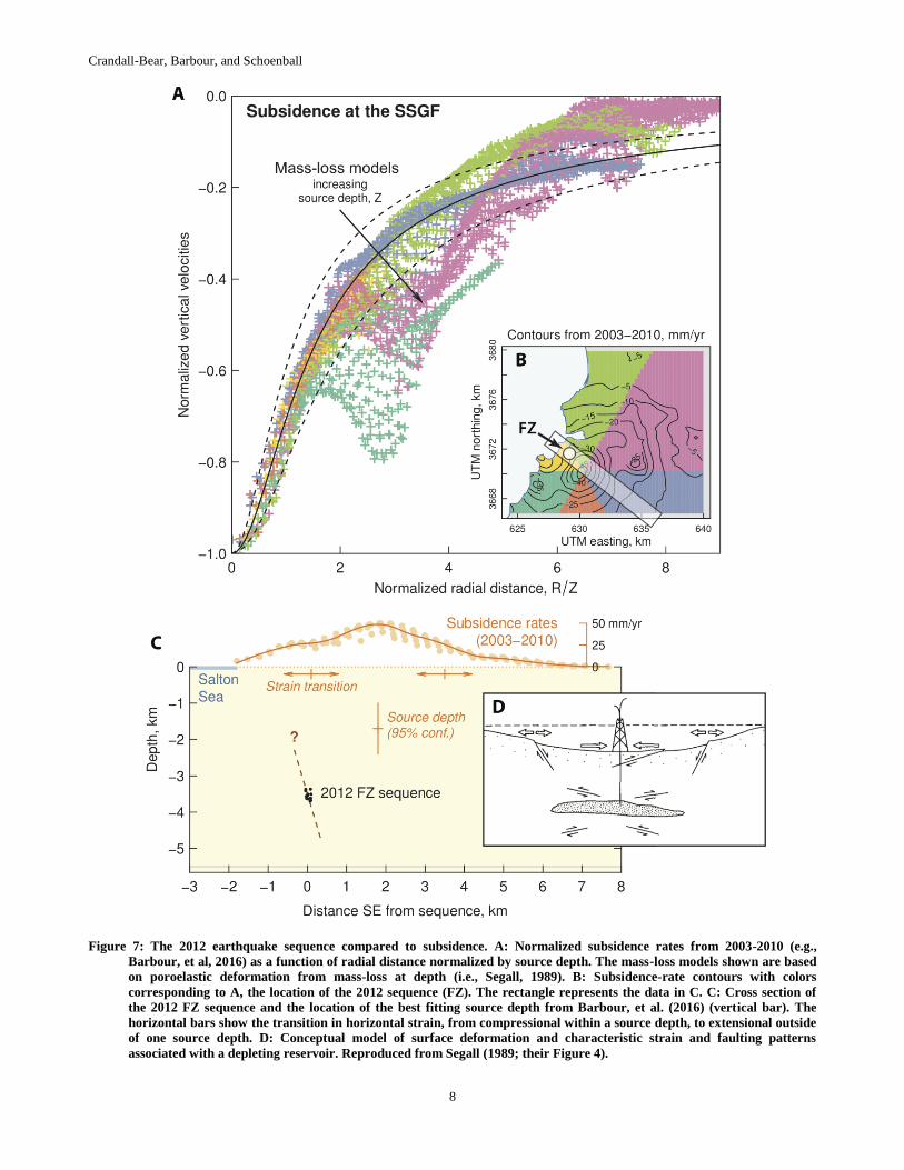
Figure 7: The 2012 earthquake sequence compared to subsidence. A: Normalized subsidence rates from 2003-2010 (e.g.,

Barbour, et al, 2016) as a function of radial distance normalized by source depth. The mass-loss models shown are based

on poroelastic deformation from mass-loss at depth (i.e., Segall, 1989). B: Subsidence-rate contours with colors

corresponding to A, the location of the 2012 sequence (FZ). The rectangle represents the data in C. C: Cross section of

the 2012 FZ sequence and the location of the best fitting source depth from Barbour, et al. (2016) (vertical bar). The

horizontal bars show the transition in horizontal strain, from compressional within a source depth, to extensional outside

of one source depth. D: Conceptual model of surface deformation and characteristic strain and faulting patterns

associated with a depleting reservoir. Reproduced from Segall (1989; their Figure 4).

Crandall-Bear, Barbour, and Schoenball

9

With the seismological data at hand, we cannot establish conclusively that depletion of the geothermal reservoir (Figure 1C) induced the

earthquake sequence in question, although it appears to have had a considerable influence on the local stress field. A few independent

observations may help illuminate the possible connection. Firstly, patterns seen in surface deformation at the SSGF are consistent with

volumetric contraction at depth from a depleting reservoir (Figure 7A; Barbour, et al., 2016) suggesting that crustal stresses are

perturbed significantly. While these strains are likely to be elastic, the decades-long trend of mass loss from the reservoir (Figure 1) all

but ensures that crustal deformation anomalies will be long-lived.

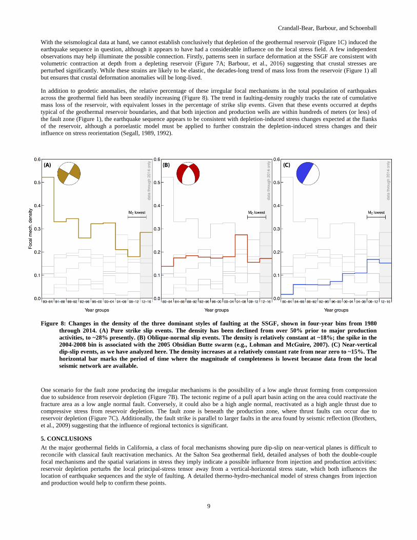
In addition to geodetic anomalies, the relative percentage of these irregular focal mechanisms in the total population of earthquakes

across the geothermal field has been steadily increasing (Figure 8). The trend in faulting-density roughly tracks the rate of cumulative

mass loss of the reservoir, with equivalent losses in the percentage of strike slip events. Given that these events occurred at depths

typical of the geothermal reservoir boundaries, and that both injection and production wells are within hundreds of meters (or less) of

the fault zone (Figure 1), the earthquake sequence appears to be consistent with depletion-induced stress changes expected at the flanks

of the reservoir, although a poroelastic model must be applied to further constrain the depletion-induced stress changes and their

influence on stress reorientation (Segall, 1989, 1992).

Figure 8: Changes in the density of the three dominant styles of faulting at the SSGF, shown in four-year bins from 1980

through 2014. (A) Pure strike slip events. The density has been declined from over 50% prior to major production

activities, to ~28% presently. (B) Oblique-normal slip events. The density is relatively constant at ~18%; the spike in the

2004-2008 bin is associated with the 2005 Obsidian Butte swarm (e.g., Lohman and McGuire, 2007). (C) Near-vertical

dip-slip events, as we have analyzed here. The density increases at a relatively constant rate from near zero to ~15%. The

horizontal bar marks the period of time where the magnitude of completeness is lowest because data from the local

seismic network are available.

One scenario for the fault zone producing the irregular mechanisms is the possibility of a low angle thrust forming from compression

due to subsidence from reservoir depletion (Figure 7B). The tectonic regime of a pull apart basin acting on the area could reactivate the

fracture area as a low angle normal fault. Conversely, it could also be a high angle normal, reactivated as a high angle thrust due to

compressive stress from reservoir depletion. The fault zone is beneath the production zone, where thrust faults can occur due to

reservoir depletion (Figure 7C). Additionally, the fault strike is parallel to larger faults in the area found by seismic reflection (Brothers,

et al., 2009) suggesting that the influence of regional tectonics is significant.

5. CONCLUSIONS

At the major geothermal fields in California, a class of focal mechanisms showing pure dip-slip on near-vertical planes is difficult to

reconcile with classical fault reactivation mechanics. At the Salton Sea geothermal field, detailed analyses of both the double-couple

focal mechanisms and the spatial variations in stress they imply indicate a possible influence from injection and production activities:

reservoir depletion perturbs the local principal-stress tensor away from a vertical-horizontal stress state, which both influences the

location of earthquake sequences and the style of faulting. A detailed thermo-hydro-mechanical model of stress changes from injection

and production would help to confirm these points.

Crandall-Bear, Barbour, and Schoenball

10

ACKNOWLEDGMENTS

The USGS 1-m LiDAR DEM is available at www.opentopography.org (https://doi.org/10.5069/G9V985ZF). Geothermal injection and

production data are from the California Department of Oil and Gas and Geothermal Resources (www.conservation.ca.gov/dog). Image

log data was downloaded from http://geosteam.conservation.ca.gov/Well/WellDetailPage.aspx?apinum=02591485. Seismological data

are from the SCEDC (http://scedc.caltech.edu) and IRIS-DMC (http://ds.iris.edu). We used HASH version 1.2 and SATSI version

140818, both available from the USGS (https://earthquake.usgs.gov/research/software). The SCEC CVM is available at

http://scedc.caltech.edu/research-tools/3d-velocity.html. This paper benefited from internal reviews by Jack Norbeck and Ole Kaven.

Any use of trade, firm, or product names is for descriptive purposes only and does not imply endorsement by the U.S. Government.

REFERENCES

Barbour, A. J., Evans, E. L., Hickman, S. H., and M. Eneva (2016). Subsidence rates at the southern Salton Sea consistent with reservoir

depletion. J. Geophys. Res., 121(7), 5308-5327, doi: 10.1002/2016JB012903

Brothers, D. S., N. W. Driscoll, G. M. Kent, A. J. Harding, J. M. Babcock, and R. L. Baskin (2009). Tectonic evolution of the Salton

Sea inferred from seismic reflection data, Nat. Geosci., 2 (8), 581–584, doi:10.1038/ngeo590

Fialko, Y., and M. Simons (2000). Deformation and seismicity in the Coso geothermal area, Inyo County, California: Observations and

modeling using satellite radar interferometry. J. Geophys. Res., 105(B9), 21781-21793, doi: 10.1029/2000JB900169

Frohlich, C. (1992). Triangle diagrams: ternary graphs to display similarity and diversity of earthquake focal mechanisms. Phys. Earth

Planet. In., 75(1-3), 193-198, doi: 10.1016/0031-9201(92)90130-N

Hardebeck, J. L., and A. J. Michael (2006), Damped regional-scale stress inversions: Methodology and examples for southern California

and the Coalinga aftershock sequence, J. Geophys. Res., 111, B11310, doi: 10.1029/2005JB004144

Hardebeck, J. L., and P. M. Shearer (2002). A new method for determining first-motion focal mechanisms. Bull. Seis. Soc. Am., 92(6),

2264-2276, doi: 10.1785/0120010200

Hardebeck, J. L., and P. M. Shearer (2003). Using S/P amplitude ratios to constrain the focal mechanisms of small earthquakes. Bull.

Seis. Soc. Am., 93(6), 2434-2444, doi: 10.1785/0120020236

Hulen, J. B., D. Kaspereit, D. L. Norton, W. Osborn, F. S. Pulka, and R. Bloomquist (2002). Refined conceptual modeling and a new

resource estimate for the Salton Sea geothermal field, Imperial Valley, California, Trans. Geotherm. Resour. Council, 26, 29–36

Kaven, J. O., Barbour, A. J., and T. Ali (2017). Constraints on geothermal reservoir volume change calculations from InSAR surface

displacements and injection and production data, EGU General Assembly Conference Abstracts, 19, p. 17875

Llenos, A. L., and A. J. Michael (2016). Characterizing potentially induced earthquake rate changes in the Brawley seismic zone,

southern California. Bull. Seis. Soc. Am., 106(5), 2045-2062, doi: 10.1785/0120150053

Lohman, R. B., and J. J. McGuire (2007). Earthquake swarms driven by aseismic creep in the Salton Trough, California. J. Geophys.

Res., 112(B4), doi: 10.1029/2006JB004596

Lund, B., & Townend, J. (2007). Calculating horizontal stress orientations with full or partial knowledge of the tectonic stress tensor.

Geophysical Journal International, 170(3), 1328-1335.

Magistrale, H., S. Day, R. W. Clayton, and R. Graves (2000). The SCEC southern California reference 3D seismic velocity model

Version 2, Bull. Seismol. Soc. Am., 90, 6B, S65-S76, doi: 10.1785/0120000510

Mastin, L. (1988). Effect of borehole deviation on breakout orientations. J. Geophys. Res., 93(B8), 9187, doi:

10.1029/JB093iB08p09187

McGuire, J. J., R. B. Lohman, R. D. Catchings, M. J. Rymer, and M. R. Goldman (2015). Relationships among seismic velocity,

metamorphism, and seismic and aseismic fault slip in the Salton Sea Geothermal Field region, J. Geophys. Res., 120, 2600–2615.

doi: 10.1002/2014JB011579

Meng, X., and Z. Peng (2014). Seismicity rate changes in the Salton Sea Geothermal Field and the San Jacinto Fault Zone after the

2010 Mw 7.2 El Mayor-Cucapah earthquake, Geophys. J. Int., 197, 3, 1750–1762, doi: 10.1093/gji/ggu085

Michael, A.J. (1984). Determination of stress from slip data: faults and folds, J. Geophys. Res., 89(B13), 11517-11526, doi:

10.1029/JB089iB13p11517

Mossop, A., and P. Segall (1999). Volume strain within the Geysers geothermal field. J. Geophys. Res., 104(B12), 29113-29131, doi:

10.1029/1999JB900284

Segall, P. (1989). Earthquakes triggered by fluid extraction. Geology, 17(10), 942-946, doi: 10.1130/0091-

7613(1989)017<0942:ETBFE>2.3.CO;2

Segall, P. (1992). Induced stresses due to fluid extraction from axisymmetric reservoirs. PAGEOPH, 139(3-4), 535-560, doi:

10.1007/BF00879950

Segall, P., and S. D. Fitzgerald (1998). A note on induced stress changes in hydrocarbon and geothermal

reservoirs. Tectonophys., 289(1), 117-128, doi: 10.1016/S0040-1951(97)00311-9

Crandall-Bear, Barbour, and Schoenball

11

Schoenball, M., and N. C. Davatzes (2017). Quantifying the heterogeneity of the tectonic stress field using borehole data. J. Geophys.

Res., 122(8), 6737–6756, doi: 10.1002/2017JB014370.

Schoenball, M., Martínez-Garzón, P., Barbour, A. J., and G. Kwiatek (2016). The Origin of High-angle Dip-slip Earthquakes at

Geothermal Fields in California. Poster Presentation at 2016 SCEC Annual Meeting

Sibson, R. H. (1985), A note on fault reactivation, J. Struct. Geo., 7(6), 751-754, doi: 10.1016/0191-8141(85)90150-6

Taira, T., Nayak, A., Brenguier, F., and M. Manga (2018). Monitoring reservoir response to earthquakes and fluid extraction, Salton Sea

geothermal field, California. Sci. Adv., 4(1), doi: 10.1126/sciadv.1701536

Vasco, D. W., J. Rutqvist, A. Ferretti, A. Rucci, F. Bellotti, P. Dobson, C. Oldenburg, J. Garcia, M. Walters, and C.

Hartline (2013), Monitoring deformation at The Geysers Geothermal Field, California using C-band and X-band interferometric

synthetic aperture radar, Geophys. Res. Lett., 40, 2567–2572, doi: 10.1002/grl.50314

Yang, W., Hauksson, E., and P. M. Shearer (2012). Computing a large refined catalog of focal mechanisms for southern California

(1981–2010): Temporal stability of the style of faulting. Bull. Seis. Soc. Am., 102(3), 1179-1194, doi: 10.1785/0120110311

Zhang, Q., G. Lin, Z. Zhan, X. Chen, Y. Qin, and S. Wdowinski (2017), Absence of remote earthquake triggering within the Coso and

Salton Sea geothermal production fields, Geophys. Res. Lett., 44, 726–733, doi: 10.1002/2016GL071964.

Zoback, M. D., Barton, C. A., Brudy, M., Castillo, D. A., Finkbeiner, T., Grollimund, B. R., … Wiprut, D. J. (2003). Determination of

stress orientation and magnitude in deep wells. International Journal of Rock Mechanics and Mining Sciences, 40(7–8), 1049–

1076. http://doi.org/10.1016/j.ijrmms.2003.07.001