Lab 2

Spectrum Analysis In the study of communication circuits and systems, frequency domain analysis techniques play a key role.The communication systems engineer deals with signal bandwidths and signal locations in the frequencydomain. The tools for this analysis are Fourier series and Fourier transforms. The types of signalsencountered can range from simple deterministic signals to very complex random signals. In thisexperiment we mostly consider deterministic signals which are also periodic. The Keysight 33600A will beused at the end of this experiment to generate more random like waveforms.

Background

Power Spectral Density of Periodic Signals In this background section we would like to connect the Fourier theory for periodic signals to themeasurements made by a spectrum analyzer. We are not only interested in the location of spectral lines,but also the amplitudes in dBm. Formally, the frequency domain representation of periodic signals can beobtained using the complex exponential Fourier series. If is periodic with period , that is

for any integer , then

where

and . By Fourier transforming (1) term-by-term using , we can write

The Fourier transform of in terms of the Fourier series coefficients is good starting point, but there is amore convenient way of obtaining the coefficients via the Fourier transform of one period of .

An alternate approach is to obtaining the Fourier transform of is to write

Lab 2 Page 1 of 27

where is one period of , i.e.,

Using the Fourier transform pair

where

we have

If we now equate (3) and (8) we see that the Fourier coefficients are simply given by

which will be very useful in calculating the power spectrum of the periodic signals considered in this lab.Since the spectrum analyzer measures the power spectral density (PSD) of a signal , we now have toconnect the Fourier transform results with the PSD theory.

For power signal , the PSD, , gives the distribution of power in versus frequency. Since is a density, it has units of W/Hz. Formally the power spectral density is defined as

where is the autocorrelation function of the signal . The autocorrelation function is computed asa time average for deterministic signals, and a statistical average for random signals. The time averagedefinition of , when is periodic with period , is

Since is periodic, it follows that is also periodic, which implies that will contain impulses.For real and periodic it is a simple matter to show that and can be written in terms of theFourier coefficients corresponding to , that is

and

Lab 2 Page 2 of 27

Note that when the PSD consists of spectral lines, the units associated with the spectral lines is actuallypower in W, not W/Hz, at least when the impedance is included in the analysis. We can now relate the PSDtheory to the actual PSD measurement in a ohm environment. Here we assume is thevoltage of a ohm source (Keysight 33600 function generator), and the load is the spectrumanalyzer, which has input impedance ohms. The theoretical power of each spectral line is

at Hz. Be careful here making sure is indeed the voltage waveform across the 50 ohm loaddriven from a 50 ohm source. This voltage is one half the open circuit voltage. A factor of 4 is needed in thedenominator of (14) . if our is the open circuit voltage. Note: The Keysight 33600 generators, when in50 ohm source mode, actually display the voltage across a 50 ohm load impedance, so there is no worryabout using the factor of 4 in your calculation. Converting to dBm would be the next step to relate theoryto measurement on the spectrum analyzer. One additional note however, is that the theoretical PSD wehave described is two-sided, while spectrum analyzer displays only the one-sided spectrum. For the case ofreal signals we know that the PSD is an even function of frequency. The power values of the spectral needto be doubled when relating to the single-sided display, or in dBm, we add 3 dB to the theoretical value,i.e.,

where , the amplitude of is the voltage across the input, and is thefundamental frequency of the generated waveform.

Pseudo-Noise Sequence Generators In the testing and evaluation of digital communication systems a source of random like binary data isrequired. A maximal-length sequence generator or pseudo-noise (PN) or pseudo-random bit sequence(PRBS) on the Keysight 33600, is a code often used for this purpose. A generator of this type produces asequences of binary digits that are periodic. For a listing of the properties of maximal-length sequences seethe Ziemer and Peterson, Digital Communications and Spread Spectrum Systems, Macmillian Publishing Co.,New York, 1985. Typical uses of PN sequences are:

Encipherment: A message written in binary digits may be added modulo-2 (exclusive-OR) to a PNsequence acting as a key. The decipherment process consists of adding the same PN sequence,synchronized with the first, modulo-2 to the encoded message. Such a technique is a form ofscrambling.Randomizer: A PN sequence can also be used for breaking up long sequences of 1's or 0's which maybias a communications channel in such a way that performance of the communications system isdegraded. The PN sequence is referred to as a \emph{randomizer}. Note that the scrambler mentionedabove and the randomizer perform the same function, but for different purposes.Testing the performance of a data communication system.Code generator.Prescribed Sequence Generator, such as needed for word or frame synchronization.

Lab 2 Page 3 of 27

Practical implementation of a PN code generator can be accomplished using an -stage shift register withappropriate feedback connections. An -stage shift register is a device consisting of consecutive binarystorage positions, typically D-type flip-flops, which shift their contents to the next element down the lineeach clock cycle. With the ready availability of programmable logic devices, it is also possible to implementthe generator as a software abstraction, e.g., assembly, C/C++, or Verilog/VHDL code (more on this later).Without feedback the shift register would be empty after clock cycles. A general feedback configurationis shown in Figure [N_stage_shift] with the input to the first stage being a logical function of the outputs ofall stages. The resulting output sequence will always be periodic with some period . The maximumsequence period is

The feedback arrangement which achieves the maximum sequence period results in a maximum lengthsequence or m-sequence. The block diagram and output sequence for a three stage m-sequence generatorare shown in Figure [ThreeStage]. The logic levels here are assumed to be bipolar ( ). In practice theactual logic levels will correspond to the device family levels. Possible exclusive-OR feedback connectionsfor m-sequences with through are given in Table [PN_Connect].

The power spectrum of the -sequence generator output can be found from the autocorrelationfunction . By definition we can write

where is the clock period. For long sequences the above integral is difficult to evaluate.

Figure 1: -stage linear feedback shift register (LFSR).

Lab 2 Page 4 of 27

Stages Connections Stages Connections

2 9

3 10

4 11

5 12

6 13

7 14

8 15

Figure 2: Three stage, length -Sequence Generator}

When writing and -sequence generator from scratch, it is important to know the shift register (SR) tapconnections that yield the maximal length. Table 1 provides these connections for 2-15 stages.

Table 1: -Sequence Generator Feedback Connections for 2 - 15 stages.

An example of how to compute for ( ) is given below. For this example a is used inplace of a for the bit , but multiplication is defined as and ,which is a bipolar AND operation. We will find the autocorrelation function at discrete times usingthe normalized correlation

where is the product of a bit in the sequence with a corresponding bit in a shifted version of thesequence. The calculation of for is shown in Figure 3. The continuousautocorrelation function follows by connecting the discrete time points together as shown in Figure 3.

Lab 2 Page 5 of 27

Figure 3: Development of the autocorrelation function for an -sequence.

Figure 4: -sequence autocorrelation function.

Logic Level Shifting

The analysis of the -sequence generator in the previous section assumed logic levels of , or moregenerally . In practice the logic levels produced by hardware will be different, say voltage levels of and for logic 0 and 1 respectively. At the waveform level we can model this by writing

where and are level shifting constants. Assuming has levels of and has levels of , itcan be shown that

Lab 2 Page 6 of 27

The autocorrelation function and power spectral density under the transformation can also be found.Starting with the autocorrelation function

Notice that the last two terms are just constants, so they will only contribute to the spectral line at ordc. The power spectral density will simply be

where . Since the spectrum analyzer does not display the dc value, we are not tooconcerned with the exact value for .

Random Binary Sequence

The extreme of the -sequence generator is a purely random sequence. To describe such a waveformrequires the concept of a random process. Without going into too much detail, we can write

where is a sequence of independent random variables, corresponding to an ideal coin-flip sequence,which takes on values of . The function is a pulse-type waveform, e.g., rectangular of duration ,which is the separation between pulses, and is a random variable independent of and uniform overthe interval . Note that versus is used to denote the fact that we are describing arandom process.

The autocorrelation function of this waveform is

where

is the pulse shape autocorrelation function, and

Lab 2 Page 7 of 27

is the random coin-toss sequence autocorrelation sequence. For a true random coin-toss sequence, theflips are equally likely and independent of each other, so

This simplifies to

Taking the Fourier transform we obtain the power spectrum

where . Due to the fact that the sequence is purely random, the power spectrum is now acontinuous function of frequency, at least in this case.

For a rectangular pulse shape, which was inherent in the -sequence discussion,

and the power spectrum is thus

The NRZ notation is explained in the next section on line codes.

As a final note, as in the case of the -sequence generator discussion, if the logic levels are shifted awayfrom we simply apply the transformation results of (23).

The Keysight 33600 does not produce pure random bit stream with its PRBS, but the you can approximate itby increasing the number of shift register stages to 32. With 32 stages the code period is (using Python):

Which is a very large period, very much like a truly random bit sequence.

Baseband Digital Data Transmission and Line Coding

Baseband digital data transmission (see Z&T Chapter 4) refers to sending digital data over a channel that iscentered in the frequency domain about DC. The physical channel here is often a cable (wire) such astwisted-pair ethernet, RS232, etc. Baseband data transmission also occurs in reading/writing to magneticstorage or free-space optical used in infrared remote controls, where the light is intensity modulated by thebaseband data.

# Sequence period for 33600A PRBS Data = PN322**32 = 4294967296

Lab 2 Page 8 of 27

As mentioned earlier, an -sequence can be used as a test data source in place of purely random data thatmay actually be sent over the channel. The format of the data may not always involve a rectangular pulseshape. The subject of line coding deals with the selection of pulse shapes and/or coding schemes, that alterthe power spectral density from what might be obtained from the simple rectangular pulse shape. Aportion of Z&T Chapter 4 is devoted to line codes and their power spectra. Figure 5 provides an example ofsix different line codes. In this lab we are only interested in NRZ change also known as NRZ (non-return-to-zero) and split-phase also known as Manchester coding.

Figure 5: Binary data formats of line codes taken from Z &T p. 217.

The natural waveform produced by the -sequence generator, discussed earlier, is the NRZ format, as wellas the PSD of [1]. To obtain Manchester from NRZ we can multiply by a square-wave clock with periodequal to the data bit duration, . The corresponding pulse shape for Manchester is (Z&T Example 4.2)

Lab 2 Page 9 of 27

We find the PSD by first finding

Since , we can write that

Since the 33600A does not natively contain Manchester line coding, you will be creating and then loadingone period of an -sequence as an arbitrary waveform (ARB) via a CSV file created in the Jupyter notebooksample. A companion NRZ waveform will also be created for comparison purposes.

Preliminary Analysis

Problem 1

Find the power spectral density of a periodic pulse train signal, period , shown in Figure 6.

Figure 6: Pulse train signal having pulse period , pulse width , and having peak amplitude of .

Assume that the waveform is delivered to a ohm load. The recommended approach is to utilizeequations (6), (9), and finally (13). The (14) gets the scaling relative to an load, i.e.,

In the laboratory exercises portion of this lab you will be comparing theory to measurement. The Jupyternotebook sample contains the helpful function line_spectra_dBm() for creating single-sided spectralplots in dBm.

def line_spectra_dBm(fn,Xn,floor_dBm = -60,R0 = 50): """ Plot the one-sided line spectra from Fourier coefficients in dBm. Inputs ------

Lab 2 Page 10 of 27

Note under the hood line_spectra_dBm() uses scikit-dsp-comm function sigsys.line_spectra() withsome scaling so that amplitude spectra in dB in converted to dBm into an R0 ohm load.

Example

fn = harmonic frequencies correspinding to Xn's Xn = pulse train FS coefficients floor_dBm = spectrum floor in dBm R0 = impedance (default 50 ohms) Returns ------- Sx_dBm = One-sided bandpass lines as dBm levels Mark Wickert February 2019 """ Xn_dBm = abs(Xn*sqrt(1000/(2*R0))) Xn_dBm[0] = abs(Xn[0])*sqrt(1000/(R0)) ss.line_spectra(fn,Xn_dBm,mode='magdB',sides=1,floor_dB=floor_dBm) ylabel(r'Power (dBm)') xlabel(r'Frequency (Hz)') title(r'Line Spectra PSD') Sx_dBm = 20*log10(2*Xn_dBm) Sx_dBm[0] -= 6.02 return Sx_dBm

n = arange(0,50)Ts = 1e-6tau = 100e-9A = 0.1Xn = A*tau/T0*sinc(n*tau/T0)*exp(-1j*2*pi*n*tau/2/T0)

Xn_dBm = line_spectra_dBm(n/Ts/1e6,Xn,floor_dBm = -60)title(r'Theory 1 MHz Pulse Train, $\tau = 100$ns, $A = 100$mV')xlabel(r'Frequency (MHz)');xlim([0,50]);

Lab 2 Page 11 of 27

Figure 7: Spectra output from line_spectra_dBm() for a 1 MHz pulse train.

Problem 2

Find the power spectral density of a coherent co-sinusoidal pulse train signal, period , shown in Figure 7.

Figure 8: Coherent co-sinusoidal pulse train signal having pulse period , exactly sinusoid cycles per period,and having peak amplitude of .

The waveform shown above is the coherent version of the co-sinusoidal signal. A non-coherent version isalso possible by simply multiplying a pulse train signal by . With this signal configuration thenumber of sinusoid cycles per pulse period is not necessarily an integer and the phase of the on eachburst may not be the same from cycle-to-cycle.

Coherent Co-Sinusoidal Case

Lab 2 Page 12 of 27

Here the task is to analyze the coherent case using the same approach as outlined in Problem 1. This is thewaveform generated by the 33600A when in burst mode. More details on setting up the generator later. Toget started your initial task is to show that

In (39) it is convenient to define

as substitutions for , respectively, when and . It then follows that

Getting is now easy to obtain. Working through the show that is tedious work.

In the laboratory exercises portion of this lab you will be comparing theory to measurement. The Jupyternotebook sample contains the helpful function coherent_cosinusoid() for calculating the Fouriercoefficients. The function line_spectra_dBm() can again be used for plotting.

def coherent_cosinusoid(f0,A,Ncyc,Ts,Nstop,Nstart=0,theta=0): """ Coherent cosinusoid pulse train Xn Fourier coefficients Inputs ------ f0 = carrier frequency in Hz A = peak amplitude (2*A = p-p) Ncyc = cycle per period Ts = pulse train period Nstop = the coefficients stop index (actually one less) Nstart = the coefficient start index (default is 0) theta = starting phase (default = 0) Returns ------- Xn = Fourier coefficients over the specified coefficient range Note: Ncyc*1/f0 must be less than Ts Mark Wickert February 2019 """ Xn = zeros(Nstop-Nstart,dtype = complex128) for n in range(Nstart,Nstop): beta = Ncyc*(1 - n/(Ts*f0)) alpha = Ncyc*(1 + n/(Ts*f0)) Xn[n-Nstart] = A*Ncyc/(2*Ts*f0)*(sinc(beta)*exp(1j*(pi*beta + theta)) \

Lab 2 Page 13 of 27

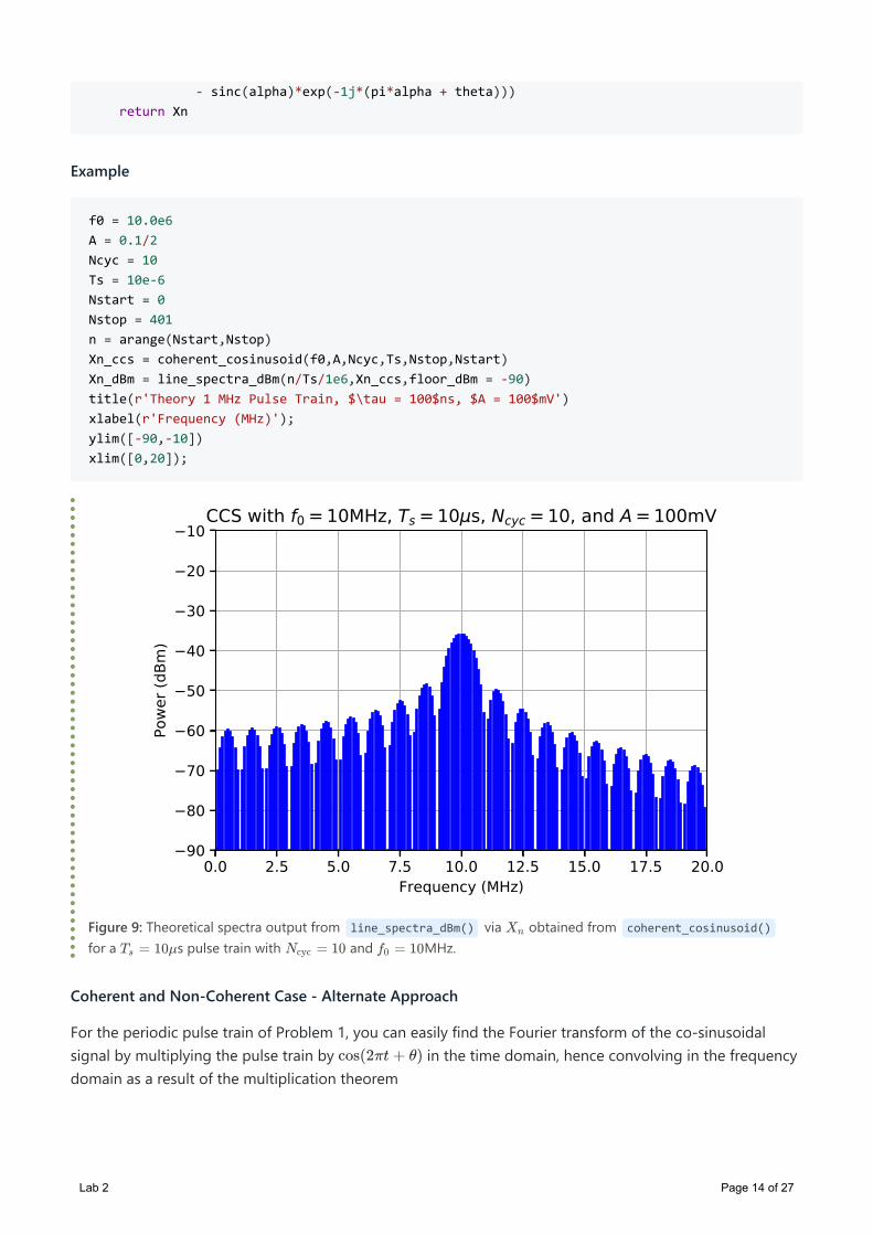
Example

Figure 9: Theoretical spectra output from line_spectra_dBm() via obtained from coherent_cosinusoid()

for a s pulse train with and MHz.

Coherent and Non-Coherent Case - Alternate Approach

For the periodic pulse train of Problem 1, you can easily find the Fourier transform of the co-sinusoidalsignal by multiplying the pulse train by in the time domain, hence convolving in the frequencydomain as a result of the multiplication theorem

- sinc(alpha)*exp(-1j*(pi*alpha + theta))) return Xn

f0 = 10.0e6A = 0.1/2Ncyc = 10Ts = 10e-6Nstart = 0Nstop = 401n = arange(Nstart,Nstop)Xn_ccs = coherent_cosinusoid(f0,A,Ncyc,Ts,Nstop,Nstart)Xn_dBm = line_spectra_dBm(n/Ts/1e6,Xn_ccs,floor_dBm = -90)title(r'Theory 1 MHz Pulse Train, $\tau = 100$ns, $A = 100$mV')xlabel(r'Frequency (MHz)');ylim([-90,-10])xlim([0,20]);

Lab 2 Page 14 of 27

The details quickly lead to

where for the standard pulse train. Since this is in the form of a line spectra, we can identifycoefficients from (44) directly and form the power spectrum directly from the average powerin each spectral line. The are not necessarily harmonically related to as are not necessarilyharmonically related. Note that the positive frequency spectrum will be composed terms from both up-shifted and down-shifted pulse train spectra, unless . For the coherent case spectral line combineaccording to the phasor additional formula.

The Jupyter notebook sample contains the function line_spectra_CS_dBm() for plotting the single-sidedline spectra. The user has to supply pulse train coefficients and harmonic frequencies in arrays.

def line_spectra_CS_dBm(f0,fn,Xn,floor_dBm = -60,R0 = 50,lm_tol=0.001): """ Plot the one-sided line spectra from Fourier coefficients in dBm for bandpass signals, e.g. when a carrier f0 is present. Carrier coherency is not required. Overlapping spectral lines folding up from f < 0 will be coherently combined if coherence withing line match tolerance lm_tol. The dBm values are also returned in an ndarray. Inputs ------ f0 = carrier frequency fn = harmonic frequencies correspinding to Xn's Xn = pulse train FS coefficients floor_dBm = spectrum floor in dBm R0 = impedance (default 50 ohms) lm_tol = line spectra combining match tolerance (default 0.001 in fn units) Returns ------- fn_BPu = Unique bandpass line frequencies Sx_dBm_BPu = One-sided bandpass lines as dBm levels (combined if possible) M_BPu = Multiplicity of line frequencies in fn_BPu (should be 1 or 2) Mark Wickert February 2019 """ Xn_dBm = abs(Xn*sqrt(1000/(2*R0))) #Xn_dBm[0] = abs(Xn[0])*sqrt(1000/(R0)) fn_BP = hstack((fn[1:]+f0,array([f0]),abs(fn[1:]-f0))) Xn_dBm_BP = hstack((Xn_dBm[1:],array([Xn_dBm[0]]),Xn_dBm[1:]))/2 # Find unique line frequencies as line overlap occurs near DC from # negative frequency spectrum. Use phasor addition to combine # the overlapping/like spectral lines. lm_tol sets matching tolerance.

Lab 2 Page 15 of 27

In order to combine terms from the negative side lapping into the positive frequency side, the Scipyfunction signal.unique_roots() is used to detect this condition and then complex add the coefficients,

of the underlying pulse train. Note under the hood line_spectra_cs_dBm() uses scikit-dsp-commfunction sigsys.line_spectra() with some scaling so that amplitude spectra in dB in converted to dBminto an R0 ohm load.

Example

fn_BPu, M_BPu = signal.unique_roots(fn_BP,tol=lm_tol, rtype='avg') Xn_dBm_BPu = zeros(len(fn_BPu),dtype = complex128) for k in range(len(fn_BPu)): idx_fn = np.nonzero(np.ravel(abs(fn_BP - fn_BPu[k])<=lm_tol))[0] Xn_dBm_BPu[k] = sum(Xn_dBm_BP[idx_fn]) ss.line_spectra(fn_BPu,Xn_dBm_BPu,mode='magdB',sides=1,floor_dB=floor_dBm) ylabel(r'Power (dBm)') xlabel(r'Frequency (Hz)') title(r'Line Spectra PSD') Sx_dBm_BPu = 20*log10(2*Xn_dBm_BPu) if fn_BPu[0] == 0: Sx_dBm_BPu[0] -= 6.02 return fn_BPu, Sx_dBm_BPu, M_BPu

n = arange(0,200)f0 = 10e6Ts = 10e-6tau = 10/f0 # Ncyc/foA = 0.1/2 # For the 33600 the sinusoial burst is typically Vp-p => Vpeak = Vp-p/2Xn_cs = A*tau/Ts*sinc(n*tau/Ts)*exp(-1j*2*pi*n*tau/2/Ts) # Pulse train Xn's

fn_u, Sx_dBm_u, M_u = line_spectra_CS_dBm(f0/1e6,n/Ts/1e6,Xn_cs,floor_dBm = -90)# fn##title(r'CCS with $f_0=10$MHz, $T_s=10\mu$s, $N_{cyc}=10$, and $A = 100$mV')xlabel(r'Frequency (MHz)');ylim([-90,-10]);xlim([0,20]);

Lab 2 Page 16 of 27

Figure 10: Theoretical spectra output from line_spectra_cs_dBm() for a s pulse train with and MHz.

Problem 3

Find the power spectral density corresponding to the periodic autocorrelation function shown in Figure 11.

Figure 11: Periodic autocorrelation function for an m-sequence generator having period MT and logic levels.

Here you take a slightly different approach to finding . Starting from the autocorrelation function is astraight shot by simply Fourier transforming using (6). This is also a homework problem assigned inSet #3 of ECE 4625. More hints will be provided for the homework problem version. Note in this problemthe logic levels that rise to the above are .

Problem 4

For the purely random bit stream waveform find the power spectral density for both NRZ and Manchesterline coding at bit rate Mbps. This is almost identical to an ECE 4625 Set #3 problem.

Lab 2 Page 17 of 27

Hints:

In working (1--3) consider Section 2.5.6 of Z&T (pp. 50--51). Also recognize that when a rectangle isconvolved with itself you get a triangle.In working (2) make use of the autocorrelation property which states that for

the autocorrelation of is related to via

The power spectral density relationship follows from the modulation theorem for Fourier transforms.

In working (3) also note that the plot in Figure 6 is valid for any sequence period, . Using the Fouriertransform pair of () we can obtain by first letting represent one period of , i.e.,

Fourier transforming results in

For general logic levels, where a logic high has amplitude and a logical low has amplitude , wejust need to utilize the results presented the Logic Level Shifting subsection. In particular the non-DCterm is scaled from the above by .In working (4) realize that the random bit stream waveform autocorrelation function is now aperiodic,so the power spectrum will be a continuous function of frequency. See the random binary sequencesubsection.

Problem 5

Find the Fourier transform, , of two popular line coding pulse shapes used in wired andwireless digital communications.

Non-Return-to-Zero (NRZ)

also seen in Figure 5. Find and plot the spectrum in dB for . In your discrete-timemodeling use samples per bit. Normalize the pulse energy to unity, i.e., choose so that

Lab 2 Page 18 of 27

This will match the sampling rate used for the arbitrary waveforms loaded into the 33600A later in thelaboratory exercises.

Split-Phase or Manchester (MAN)

as seen in Figure 5. Find and plot the spectrum in dB for . Again normalize the pulseenergy to unity as in the NRZ case.

Laboratory Exercises

Periodic Pulse Train

Part a

Using one channel of the Keysight 33600A generator record time domain and frequency domain data usingthe Agilent MSO-X-6004A oscilloscope and the Keysight N9914A FieldFox spectrum analyzer respectively,for several different duty cycles . As a matter of convenience select as an integer number ofgraticule lines on the oscilloscope screen.

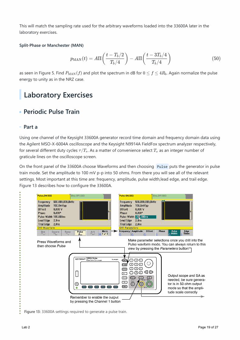
On the front panel of the 33600A choose Waveforms and then choosing Pulse puts the generator in pulsetrain mode. Set the amplitude to 100 mV p-p into 50 ohms. From there you will see all of the relevantsettings. Most important at this time are: frequency, amplitude, pulse width,lead edge, and trail edge.Figure 13 describes how to configure the 33600A.

Figure 13: 33600A settings required to generate a pulse train.

Lab 2 Page 19 of 27

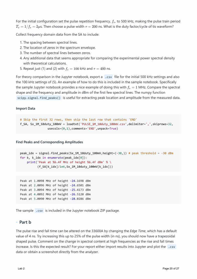
For the initial configuration set the pulse repetition frequency, , to 500 kHz, making the pulse train periods. Then choose a pulse width ns. What is the duty factor/cycle of tis waveform?

Collect frequency domain data from the SA to include:

1. The spacing between spectral lines.2. The location of zeros in the spectrum envelope.3. The number of spectral lines between zeros.4. Any additional data that seems appropriate for comparing the experimental power spectral density

with theoretical calculations.5. Repeat just (1) and (2) with kHz and ns.

For theory comparison in the Jupyter notebook, export a .csv file for the initial 500 kHz settings and alsothe 100 kHz settings of (5). An example of how to do this is included in the sample notebook. Specificallythe sample Jupyter notebook provides a nice example of doing this with MHz. Compare the spectralshape and the frequency and amplitude in dBm of the first few spectral lines. The numpy functionscipy.signal.find_peaks() is useful for extracting peak location and amplitude from the measured data.

Import Data

Find Peaks and Corresponding Amplitudes

The sample .csv is included in the Jupyter notebook ZIP package.

Part b

The pulse rise and fall time can be altered on the 33600A by changing the Edge Time, which has a defaultvalue of 4 ns. Try increasing this up to 25% of the pulse width (in ns), you should now have a trapezoidalshaped pulse. Comment on the change in spectral content at high frequencies as the rise and fall timesincrease. Is this the expected result? For your report either import results into Jupyter and plot the .csv

data or obtain a screenshot directly from the analyzer.

# Skip the first 32 rows, then skip the last row that contains 'END'f_SA, Sx_1M_10duty_100mV = loadtxt('PULSE_1M_10duty_100mV.csv',delimiter=',',skiprows=32, usecols=(0,1),comments='END',unpack=True)

peak_idx = signal.find_peaks(Sx_1M_10duty_100mV,height=(-30,)) # peak threshold = -30 dBmfor k, k_idx in enumerate(peak_idx[0]): print('Peak at %6.4f MHz of height %6.4f dBm' % \ (f_SA[k_idx]/1e6,Sx_1M_10duty_100mV[k_idx]))

Peak at 1.0098 MHz of height -24.1698 dBmPeak at 2.0096 MHz of height -24.6501 dBmPeak at 3.0094 MHz of height -25.4173 dBmPeak at 4.0092 MHz of height -26.5120 dBmPeak at 5.0090 MHz of height -28.0286 dBm

Lab 2 Page 20 of 27

Periodic Cosinusoidal Pulse Train

Part a

A periodic co-sinusoidal pulse train can be generated using the Keysight 33600A in Burst Mode. The setupsteps are described in Figure 14.

Figure 14: 33600A 33600A settings required to generate a co-sinusoidal pulse train.

To get started press the Waveform and choose Sine. Set the frequency to MHz. Then press the Burtbutton and set the number of cycles per burst, , and the burst period to s.

1. Look at the waveform on the scope to verify that exactly five cycles are contained in the burst.2. Also verify from the scope that the burst period is indeed s.3. Study the spectrum and see that the spectral nulls are located as expected4. Study the spectrum and see that the minimum line spacing is as expected.5. Repeat steps 1-4 with .6. Repeat steps 1-4 with .

Import one of the three cases into the Jupyter notebook via a .csv export from the N9914A.Compare the theoretical expectations to the measured using the Python functions found in the samplenotebook. Use a frequency span of 1 kHz to 10 MHz. To plot the theoretical power spectrum use thefunction pair

as described in the Preliminary Analysis section of this document.

Xn_ccs = coherent_cosinusoid(f0,A,Ncyc,Ts,Nstop,Nstart)Xn_dBm = line_spectra_dBm(n/Ts/1e6,Xn_ccs,floor_dBm = -90)

Lab 2 Page 21 of 27

Part b

Return and experiment with changes to . Specifically move down to 4 MHz and then up to 6MHz. Compare the experimental spectrum captured via a .csv with the theoretical expectations for each

value.

1. Note in particular that the spectrum peak shifts accordingly.2. Check to see that the pulse train characteristics of spectral nulls and minimum line spacing remain

invariant under changes in .

Part c

Using the Python function line_spectra_CS_dBm() driven by pulse train Fourier coefficients, , chose avalue for that makes the co-sinusoidal signal non-coherent. See if you can observe the spectral linesplitting apart. I want you see if a value of will make the spectral lines lapping up from the negativefrequency axis to the positive frequency axis can be made to interleave the native positive frequency axisspectral lines. Your Jupyter notebook will ultimately contain a spectrum exhibiting this behavior. Note the33600A only produces coherent co-sinusoidal signals, as far as I have been able to observe.

Pseudo-Noise (PN) Sequence Generators (PRBS) In this portion of the experiment you will verify some of the properties of PN sequence generators,specifically m-sequences. You will also consider random sequences and the impact of line coding,specifically non-return-to zero (NRZ) versus Manchester. The -sequence generator will be implementedusing the capabilities of the 33600A. To implement line coding the arbitrary waveform capability (ARB) willbe utilized.

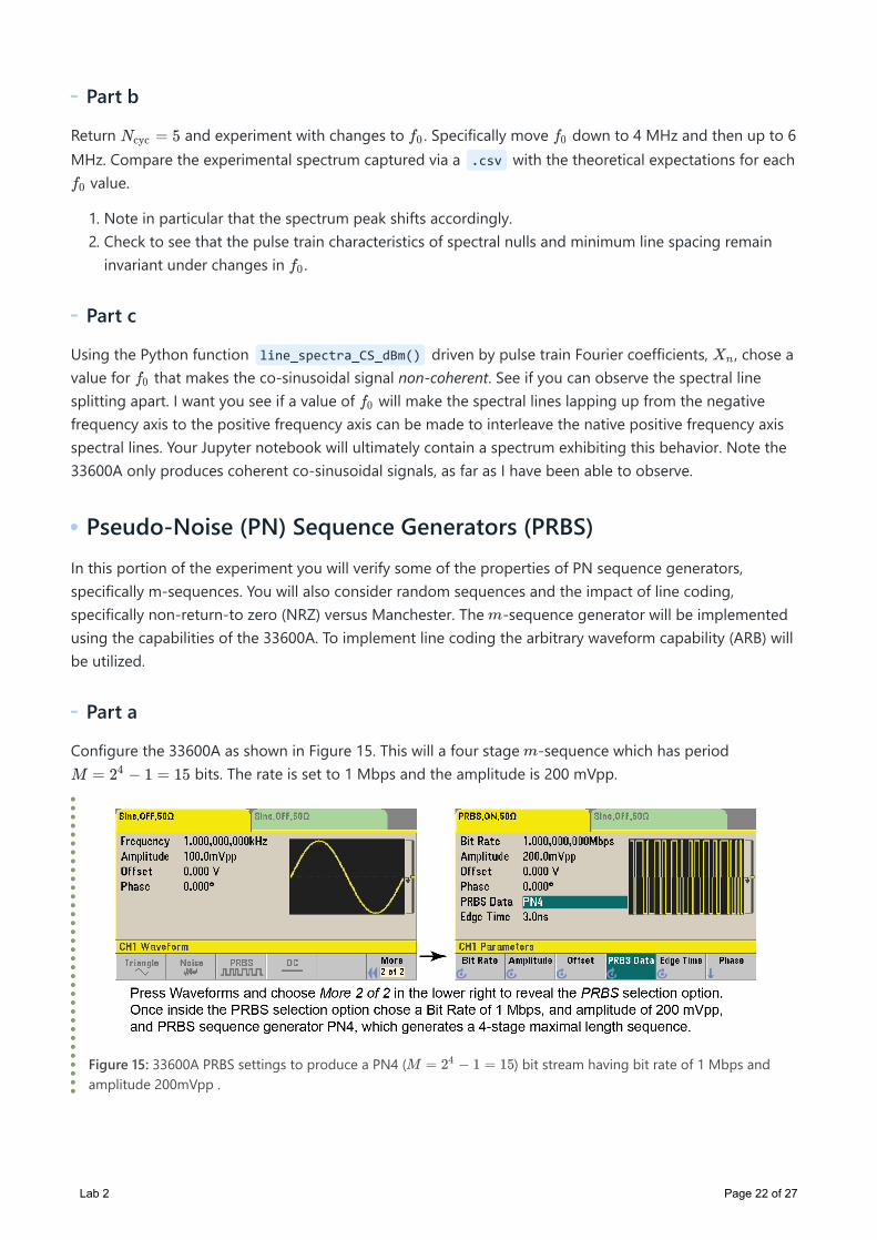
Part a

Configure the 33600A as shown in Figure 15. This will a four stage -sequence which has period bits. The rate is set to 1 Mbps and the amplitude is 200 mVpp.

Figure 15: 33600A PRBS settings to produce a PN4 ( ) bit stream having bit rate of 1 Mbps andamplitude 200mVpp .

Lab 2 Page 22 of 27

When viewing the output of pseudo random sequence generators on the scope, e.g., the MSO-X 6004A, itimport to use the generator trigger waveform to ensure a stable data stream can be observed. Figure 16shows how to set this up for observing both the time domain waveform and the power spectrum on the SA.

Figure 16: 33600A PRBS settings and measurement interconnects for the case PN4.

A property of -sequences is that once per period a sequence of ones match the shift register length mustbe present. In the miniature scope waveform of Figure 16 we see a block of 4-ones repeat three timesacross the trace, perfectly aligned with trigger waveform (the green trace). Note be sure to set the scope totrigger on the Trigger waveform output from the 33600A. You will taking at PN5 and PN10 waveforms andwill have great difficulty syncing the scope without the use of the trigger signal.

To complete Part a change the generator to PN5 and observe:

1. On the scope the occurrence of 5-ones in a row once over the sequence period2. On the spectrum analyzer verify the location of the spectral nulls3. Verify the minimum line spacing is as expected for a generator.

Part b

Change the generator to PN10 and repeat the measurements of Part a.

Part c: Almost Random Sequence Generator

Change the generator to PN32, which is the largest shift register length available on the 33600A. Observethe spectrum on the N9914A. As you zoom in to a single spectral lobe and then reduce the resolutionbandwidth see if you can resolve the spectral lines. What is the period of the PN32 generator in seconds?

Lab 2 Page 23 of 27

Part d: Arbitrary Waveform and Line Coding

For this experiment you will utilize the arbitrary waveform (ARB) capability of the 33600A to playback twodifferent 63-bit m-sequence waveforms. In general a PN sequence or PRBS, as referred to by the 33600A,has mathematical form

where is the bit period and is the serial bit rate of bit stream. The pulse shapes of interesthere are NRZ and MAN as defined earlier. The form a sequence of bits that repeat with period .

Creating ARB waveforms is easy and is described in the Jupyter notebook sample and also in a KeysightARB creation application note. The files NRZ.csv and MAN.csv are contained in the Jupyter notebooksample ZIP file. These files correspond to a -sequence waveform like (62) at 100 samples per bit,e.g.,

Loading New ARB .csv Files into the 33600A

When ARB file is first created in .csv form it has to be loaded, and in a sense compiled by the 33600Ainto a .arb file that will allow *waveform playback in a repeating loop. Figure 17 shows the steps requiredto do this. Note: You will need a flash drive to move the .csv from your computer to the 33600A.

# Desire Rb = 1 Mbps with 100x oversamplingfs = 100e6 # this parameter is entered on the 33600A# Samples per bitNs = 100# One sample per bit M = 63 bit long m-sequenceN_STAGE = 4# Use the PN_gen (M-seq) function ss over the bitwise_PNPN_63 = ss.PN_gen(2**N_STAGE - 1, N_STAGE)# Upsample and make rectangular pulse shaped bits bipolarx_NRZ = signal.lfilter(ones(Ns),1,ss.upsample(2*PN_63-1,Ns))

# Create an Ns period squarewave clock to convert NRZ to Manchestern = arange(len(x_NRZ))x_CLK = sign(cos(2*pi*1e6/fs*n))# Multiply the clock by the NRZ waveformx_MAN = x_NRZ*x_CLK

savetxt('NRZ.csv', x_NRZ, delimiter=',')savetxt('MAN.csv', x_MAN, delimiter=',')

Lab 2 Page 24 of 27

Figure 17: Copying a .csv file from USB flash to the 33600A.

Lab 2 Page 25 of 27

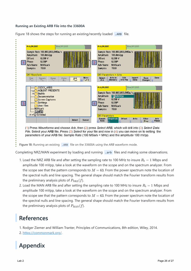
Running an Existing ARB File into the 33600A

Figure 18 shows the steps for running an existing/recently loaded .ARB file.

Figure 18: Running an existing .ARB file on the 33600A using the ARB waveform mode.

Completing NRZ/MAN experiment by loading and running .arb files and making some observations.

1. Load the NRZ ARB file and after setting the sampling rate to 100 MHz to insure Mbps andamplitude 100 mVpp, take a look at the waveform on the scope and on the spectrum analyzer. Fromthe scope see that the pattern corresponds to . From the power spectrum note the location ofthe spectral nulls and line spacing. The general shape should match the Fourier transform results fromthe preliminary analysis plots of .

2. Load the MAN ARB file and after setting the sampling rate to 100 MHz to insure Mbps andamplitude 100 mVpp, take a look at the waveform on the scope and on the spectrum analyzer. Fromthe scope see that the pattern corresponds to . From the power spectrum note the location ofthe spectral nulls and line spacing. The general shape should match the Fourier transform results fromthe preliminary analysis plots of .

References1. Rodger Ziemer and William Tranter, Principles of Communications, 8th edition, Wiley, 2014.2. https://commonmark.org/.

Appendix

Lab 2 Page 26 of 27

Capturing Screenshots from the Keysight 33600A TBD

Deleting ARB and Screen Shots from the Keysight 33600A TBD

Lab 2 Page 27 of 27