1

Spring 2018Instructor: Kai Sun

ECE 522 Power Systems Analysis II

3.3 ‐ Voltage Stability

2

Content

• Basic concepts– Voltage collapse, Saddle‐node bifurcation, P‐V curve and V‐Q curve

• Voltage Stability Analysis (VSA)– Dynamic and Static Analyses, Modal analysis and Continuation powerflow

• Causes and prevention of voltage instability

• References:1. Chapter 14 of Kundur’s book2. “Survey of the voltage collapse phenomenon”, NERC Interconnection Dynamics Task 

Force Report, Aug. 19913. EPRI Tutorial’s Chapter 64. Carson W. Taylor, “Power System Voltage Stability” McGraw Hil, 19945. “Voltage Stability Assessment: Concepts, Practices and Tools”, IEEE‐PES Power 

Systems Stability Subcommittee Special Publication, Aug. 20026. V. Ajjarapu, C. Christy, “The continuation power flow: a tool for steady state voltage 

stability analysis”, IEEE Trans Power Syst., vol. 7, no. 1, Feb, 1992

3

Voltage Stability

•Voltage stability is concerned with the ability of a power system to maintain acceptable voltages at all buses in the system under normal conditions and after being subjected to a disturbance.

•An extreme type of voltage instability is voltage collapse, in which a significant part of the system experiences a progressive and uncontrollable decline in voltage until power outages.

•Heavily loaded/stressed areas are more prone to voltage instability. 

•The main factor causing voltage instability in a power system is the inability to meet the demand for reactive power

4

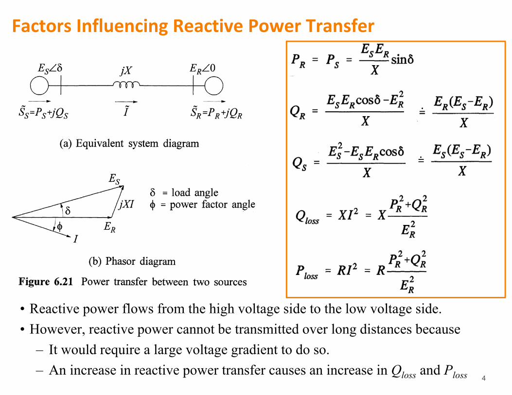
Factors Influencing Reactive Power Transfer

• Reactive power flows from the high voltage side to the low voltage side.• However, reactive power cannot be transmitted over long distances because

– It would require a large voltage gradient to do so.– An increase in reactive power transfer causes an increase in Qloss and Ploss

5

Voltage Stability vs. Rotor Angle stability

• Rotor angle stability is basically stability with generators while voltage stability is basically stability with loads– Rotor angle stability is often concerned with remote power plants connected to a large 

system over long transmission lines.– Voltage stability is concerned with load areas and load characteristics. In a large 

interconnected system, voltage collapse of a load area is possible without loss of synchronism of any generators.

• Transient voltage stability is usually closely associated with transient rotor angle stability. If voltage collapses at a point (e.g. the center of oscillation) in a transmission system remote from loads, it is, in nature, angle instability.

6

A radial system

where

ZLD decreases (with constant ZLN)

| | S

LN LD

EI IZ Z

2 2( cos cos ) ( sin sin )S

LN LNLD LDZE

Z Z Z

1 S SSC

LN LN

E EI IZ ZF

2

1 2 cos( )LN

LD

LN

LDZ ZFZ Z

• How does VR change when PR increases?

DR LV IZ cosR RP V I

1 LDR LD S S

LN

ZV Z I E EZF

2

2 def

cos cos

cos 2 1 cos( )

SLDR R

LN

SRMAX

LN

EZP V IF Z

E PZ

7

Load increases (ZLD decreases)

How does voltage instability happen?• Voltage stability depends on the

dynamics or controls with loads• Under normal conditions, ZLD>> ZLN

and an increase in active load PR usually comes with a decrease in ZLD

• However, when ZLD<ZLN (heavily loaded), a decrease in ZLD reduces PR, so any load control that maintains the load by decreasing ZLD becomes unstable.– For instance, consider a load supplied

through an ULTC transformer. When the tap-changer tries to raise the load voltage (absorbing more Mvar from the primary side of the transformer), it has the effect of reducing the effective ZLD and in turn further lowers VR seen from the primary side. That may lead to a progressive reduction of voltage if the primary side is weak in terms of reactive power.

8

Constant P

PR=P

Constant Z

PR=aVR2

• The voltage collapse at the critical point (also called the “nose” or “knee” point) is referred to as “saddle-point bifurcation”

• Does voltage collapse necessarily occur at the critical point?

ZLD decreases (assume constant ZLN)

P‐V Curve

General load

9

Saddle‐node bifurcation

• A saddle-node bifurcation is the disappearance of a system’s equilibrium as parameters change slowly (system dynamics can be ignored).

• This is an inherently nonlinear phenomenon and cannot occur in a linear model.

Saddle-node bifurcation at pmax

Equilibria disappear

Two equilibriums

P- curve

P-V curve

p+jq

pmax

Stable node

Saddle point

10

Normalized P‐V curves (various power factors)• Normally, only the operating points above the critical points represent

satisfactory operating conditions

Increase in QR (decrease of )

11

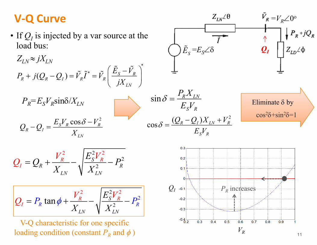
V‐Q Curve• If QI is injected by a var source at the

load bus:ZLN jXLN

**( ) S R

R R I R RLN

E VP j Q Q V I VjX

=VR0o

=ES QI

2cosS R RR I

LN

E V VQ QX

PR=ESVRsin/XLN

2( )cos R I LN R

S R

Q Q X VE V

sin R LN

S R

P XE V

22

2

22RR

R RLN LN

ISE VV P

X XQ Q

Eliminate by

cos2+sin2=1

SE

22

2

22

tan S

LN

RRRI R

LN

P E VVQX X

P QI

VR

V-Q characteristic for one specific loading condition (constant PR and )

PR increases

12

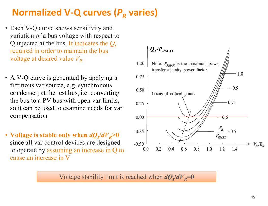
Normalized V‐Q curves (PR varies)

Voltage stability limit is reached when dQI/dVR=0

QI /PRMAX

• Each V-Q curve shows sensitivity and variation of a bus voltage with respect to Q injected at the bus. It indicates the QIrequired in order to maintain the bus voltage at desired value VR

• A V-Q curve is generated by applying a fictitious var source, e.g. synchronous condenser, at the test bus, i.e. converting the bus to a PV bus with open var limits, so it can be used to examine needs for varcompensation

• Voltage is stable only when dQI/dVR>0 since all var control devices are designed to operate by assuming an increase in Q to cause an increase in V

13

An example on Kundur’s Pages 963‐966

PAera 1 - V530

Uniformly scale up the area load with constant

A

B

C

• Probable remedial actions before C is reached Strategy 1: Inject Q at Bus 530 to increase VStrategy 2: Reduce load near Bus 530

14

Influence of Generation Characteristics

• Actions of generator AVRs provide the primary sources of voltage support

• Under normal conditions, generator terminal voltages are maintained constant

• During conditions of low/high voltages, the var output of a generator may reach its limit. Consequently, the terminal voltage is not longer maintained constant

• Then, with constant field current, the point of constant voltage is now Eq of the generator behind its synchronous reactance XSXq. That increases the network reactance significantly to further aggravate the voltage collapse condition

• It is important to maintain voltage control capabilities of generators

• The degree of voltage stability cannot be judged based only on how close the bus voltage is to the normal voltage level

Voltage collapse due to the var limit or current limit being reached is referred to as “limit-induced bifurcation”

15

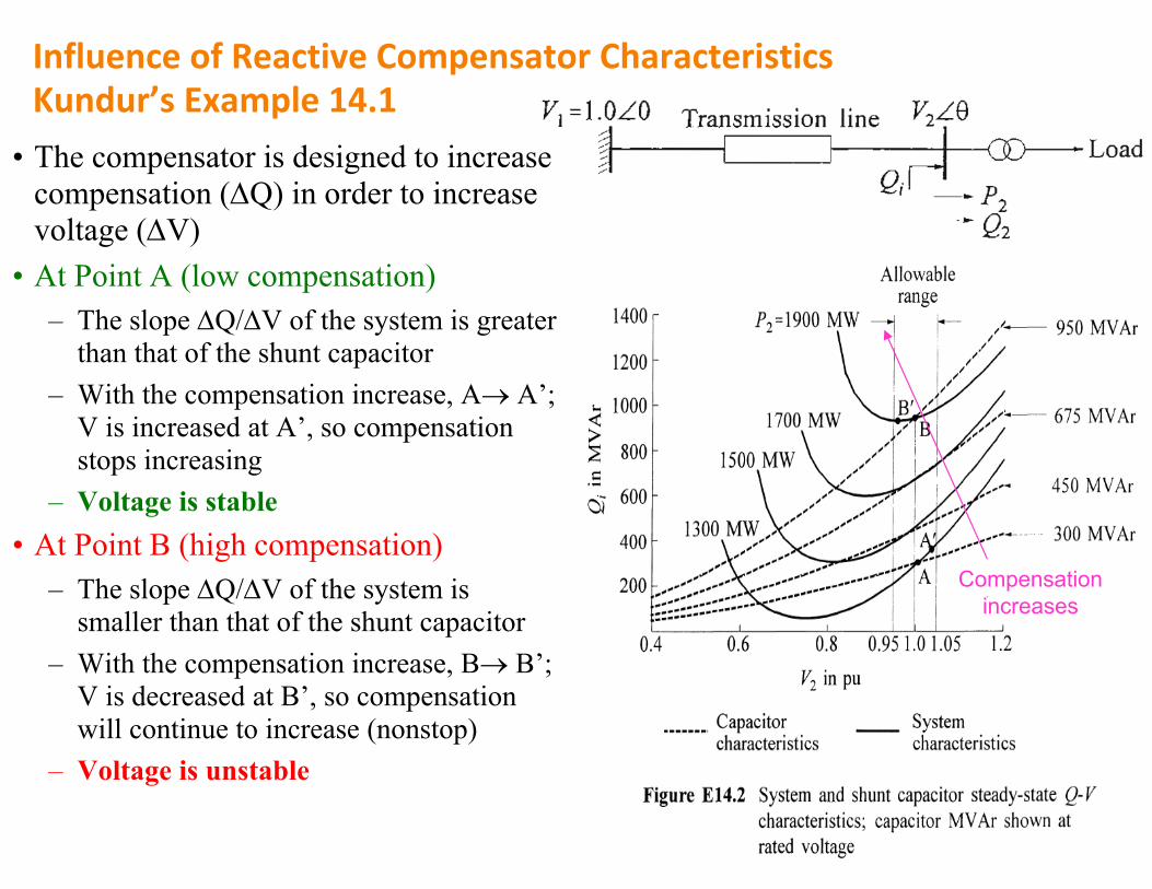
Influence of Reactive Compensator CharacteristicsKundur’s Example 14.1

Compensation increases

• The compensator is designed to increase compensation (Q) in order to increase voltage (V)

• At Point A (low compensation)– The slope Q/V of the system is greater

than that of the shunt capacitor– With the compensation increase, A A’;

V is increased at A’, so compensation stops increasing

– Voltage is stable• At Point B (high compensation)

– The slope Q/V of the system is smaller than that of the shunt capacitor

– With the compensation increase, B B’; V is decreased at B’, so compensation will continue to increase (nonstop)

– Voltage is unstable

16

• Approach:– Sensitivity and modal analysis on the powerflow model (read Kundur’s 14.3.3– Generalization of the conclusion “voltage stability limit is reached when

dQI/dVR=0 at the load bus” on a radial system

• Linearize the power flow model for a specific operating condition. Elements of the Jacobian matrix give the sensitivity between power and voltage changes.

Let P=0,

JR is the reduced Jacobian matrix of the system and represents the linearized relationship between incremental changes in bus voltage magnitudes and bus reactive power injections

Steady‐State Voltage Stability Analysis on a General Power System

17

• Voltage stability characteristics of the system can be identified by computing the eigenvalues and eigenvectors of JR

(note: =-1)

For a 3-bus system:

18

• If i>0, the ith modal voltage and the ith modal reactive power variations are along the same direction, indicating that the system is voltage stable

• If i<0, the ith modal voltage is unstable• If i=0, the ith modal voltage collapses since any small change in that modal

reactive power causes infinite change in the modal voltage• The magnitude of i determines the proximity to instability

• This is a generalization of the conclusion “voltage stability limit is reached when dQI/dVR=0 at the load bus” on a radial system

Steady‐State Voltage Stability Criteria

19

Bus Participation Factors

• The relative participation of bus k in mode i is given by

• Pki determines the contribution of i to the V-Q sensitivity at bus k• Bus participation factors determine the critical buses and areas associated with

each mode• The size of bus participation in a given mode indicates the effectiveness of

remedial actions applied at that bus in stabilizing the mode• Localized modes: very few buses with large participations• Not localized modes: many buses have small but similar degree of participations.• In practice, it is seldom necessary to compute more than 5-10 of the smallest

eigenvalues to identify all critical modes.• Also see participation factors of branches and generators in Kundur’s 14.3.3

20

Continuation Powerflow (CPF) Analysis

• Conventional powerflow algorithms are prone to divergence problems at operating conditions near the stability limit because the powerflow Jacobian matrix becomes singular at the voltage stability limit (nose point)

• The continuation powerflow (CPF) method based on the work by Ajjarapu and Christy in 1992 [6] overcomes this problem by reformulating the powerflowequations so that they remain well‐conditioned at all possible loading conditions– Able to solve power flows for stable as well as unstable equilibrium points– Locally‐parameterized continuation method, which belongs to a general class of methods for solving nonlinear algebraic equations known as path‐following methods

21

1. From an initial solution A, a tangent predictor is used to estimate B for a specified pattern of load increase.

2. Then, a corrector step determines the exact solution C using a conventional powreflow analysis with the system load assumed to be fixed.

3. The voltages for a further increase in load are then predicted based on a new tangent predictor

4. If the new estimated load D is now beyond the maximum load on the exact solution, a corrector step with loads fixed would not converge; therefore, a corrector step with a fixed voltage at the monitored bus is applied to find the exact solution E

5. As the voltage stability limit is reached, to determine the exact maximum load, the size of load increase has to be reduced gradually during the successive predictor step

See mathematical formulation in Kundur’s 14.3.5

CPF algorithm

22

Complementary use of conventional and continuation powerflowmethods

• Continuation methods are robust and flexible and ideally suited for solving powerflow problem with convergence difficulties; however, it is very slow and time‐consuming

• The best overall approach for computing powerflow solutions up to and beyond the critical point is to use the two methods in a complementary manner– Usually the conventional methods (N‐R or Fast Decoupled)  can be sued to provide solutions right up to the critical point

– The continuation methods become necessary only if solutions exactly at and past the critical point are required

23

Voltage Stability Analysis by Time‐Domain SimulationKundur’s Example 14.2

•Models:– 6 transformers (1 ULTC)– 3 shunt capacitor (buses 7, 8 & 9)– Detailed G2 and G3 with thyristor exciters– 1 over‐excitation limiter (OXL) with G3– Load 11: 50% Impedance + 50% Current– Load 8: a) constant P&Q; b) induction motor; c) constant Q + thermostatic P

• Load levels: 1. 6655MW+1986Mvar2. 6755MW+2016Mvar3. 6805MW+2031Mvar 

24

Constant P&Q load at bus 8

• Load level 1:– The ULTC of T6 restores bus 11 voltage at about 40s

• Load level 2:– While the ULTC of T6 tries to restore bus 11 voltage, the field current limit of  G3 

is met and the OXL ramps the field current down starting around 180s.• Load level 3:

– The field current of G3 reaches its limit at about 50s– Bus 11 voltage drops with each tap movement of the ULTC of  T6– The voltage settles when the ULTC  reaches its limit and stops

25

Induction motor load at bus 8• The motor stalls at about 65s, draws rapidly increased reactive power and leads to voltage collapse.

26

Thermostatically controlled load at bus 8• The load controller increases the conductance to restore the load and results in a lower bus 11 voltage

27

Causes of voltage instability• A typical scenario on the principal driving force for voltage instability:

– In response to a disturbance, power consumed by loads tends to be restored by motor slip adjustment, distribution voltage regulators and thermostats

– Restored loads increase stress on the high‐voltage network causing further voltage reduction

– Voltage instability occurs when load dynamics attempt to restore power consumption beyond the capability of the transmission network

• Principal causes– The load on transmission lines is too high– The voltage sources are too far from load centers– The source voltages are too low– There is insufficient load reactive compensation

• Contributing factors– Generator reactive power and voltage control limitations– Load Characteristics– Distribution system voltage regulators and transformer tap‐changer actions– Reactive power compensating device characteristics

28

A Typical Scenario of Short‐Term Voltage Instability

•The power system is operating in a stressed condition during hot weather with a high level of air conditioning load

•The triggering event is a multi‐phase fault near a load center– Causes voltage dips at distribution buses– Air conditioner compressor motors decelerate, drawing high current

•Following fault clearing with transmission/distribution line tripping motors draw very high current while attempting to reaccelerate. Motors stall if the power system is weak.

•Under‐voltage load rejection may not be fast enough to be effective

•Loss of much of the area load and voltage collapse

29

112

3

112

33

1GW generation tripped by SPS

4

44

Faulty zone 3 relay

5

5

6 8

6 7

7

8

Loss of key hydro units

9

9

10

Tree contact

and relay

mis-opt.

Example of Voltage Collapse: July 2nd, 1996 Western

Cascading Event

Tripped by Zone 3 relay

30

•On July 3rd, 1996, i.e. the following day, – A similar chain of events happened to cause voltages in Boise area to decline. 

– Different from the previous day, Idaho Power Company system operators noted  the declining voltages and immediately took the only option available: shedding of Boise area load

– Then, the system returned to normal within 1 hour

•Lessons learned:– The July 2nd and 3rd events in Boise, Idaho area emphasize the need for effective and sufficient, rapidly responsive dynamic Mvar reserve.

– The July 3rd events illustrate the importance of system operators’ situational awareness and rapid responses.

31

Prevention of Voltage CollapseRead Kundur’s Chapter 14.4• Application of var compensating devices

– Ensure adequate stability margin (MW & Mvar distances to instability) by proper selection of schemes

– Selection of sizes, ratings and locations of the devices (especially for dynamic reactive reserves, e.g. synchronous condensers, STATCOM and SVCs) based on a detailed study

– Design criteria based on maximum allowable voltage drop following a contingency are often not satisfactory from voltage stability viewpoint

– Important to recognize voltage control areas and weak boundaries (buses with high participation factors associated with a voltage instability mode).

• Control of transformer tap changers– Can be controlled either locally or centrally– Where tap changing is detrimental, a simple method is to block tap changing when the source side sags and unblock when voltage recovers

– Use the knowledge of load characteristics to improve the control schemes

– Microprocessor‐based ULTC controls

32

Prevention of Voltage Collapse

• Control of network voltage and generator reactive output– Improvement on AVRs, e.g. adding load (or line drop) compensation– Secondary coordinated outer loop voltage control (e.g. the hierarchical, automatic 2‐3 layers voltage control)

• Coordination of protections/controls– Ensure adequate coordination based on dynamic simulation studies– Tripping of equipment to protect from overloaded conditions should be the last resort. The overloaded conditions could be relieved by adequate control measures before isolating the equipment.

•Under‐voltage load shedding (UVLS)– To cater for unplanned or extreme situations; analogous to UFLS– Provide a low‐cost means of preventing widespread system collapse– Particularly attractive if conditions leading to voltage instability are of low probability but consequences are high

– Characteristics and locations of the loads to be shed are more important for voltage problems than for frequency problems

– Should be designed to distinguish between faults, transient voltage dips, and low voltage conditions leading to voltage collapse