ece580 guest-lecture f2011 - classesclasses.engr.oregonstate.edu/eecs/fall2017/ece580... · prof....
TRANSCRIPT
1
Prof. Andreas Weisshaar ― ECE580 Network Theory - Guest Lecture ― Fall Term 2011 1
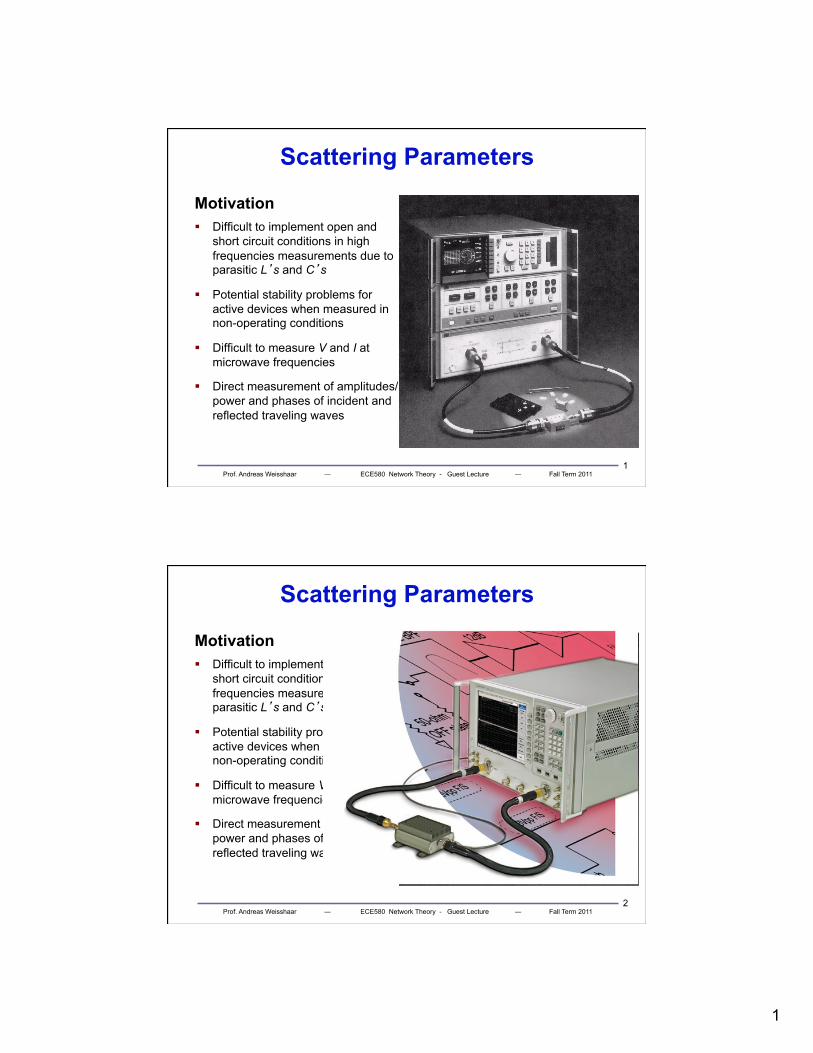
Scattering Parameters
Motivation § Difficult to implement open and
short circuit conditions in high frequencies measurements due to parasitic L’s and C’s
§ Potential stability problems for active devices when measured in non-operating conditions
§ Difficult to measure V and I at microwave frequencies
§ Direct measurement of amplitudes/power and phases of incident and reflected traveling waves
Prof. Andreas Weisshaar ― ECE580 Network Theory - Guest Lecture ― Fall Term 2011 2
Scattering Parameters
Motivation § Difficult to implement open and
short circuit conditions in high frequencies measurements due to parasitic L’s and C’s
§ Potential stability problems for active devices when measured in non-operating conditions
§ Difficult to measure V and I at microwave frequencies
§ Direct measurement of amplitudes/power and phases of incident and reflected traveling waves
2
Prof. Andreas Weisshaar ― ECE580 Network Theory - Guest Lecture ― Fall Term 2011 3
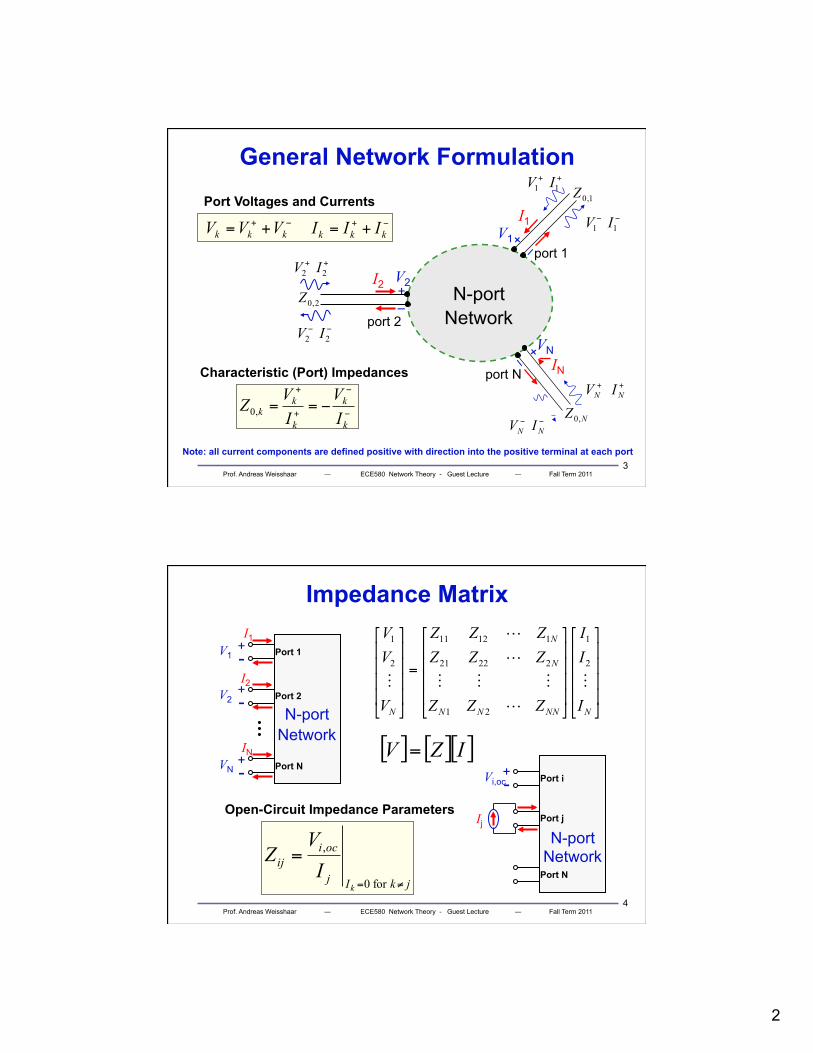
General Network Formulation
−
−
+
+
−==k
k
k
kk I
VIVZ ,0
Characteristic (Port) Impedances
−+ += kkk VVV −+ += kkk IIIPort Voltages and Currents
+ –
port 1
port 2
port N
+ – I2
I1
IN
V2
V1
VN
Note: all current components are defined positive with direction into the positive terminal at each port
−−22 IV
++22 IV
2,0Z
++NN IV
−−NN IV NZ ,0
++11 IV
−−11 IV
1,0Z
N-port Network
Prof. Andreas Weisshaar ― ECE580 Network Theory - Guest Lecture ― Fall Term 2011 4
Impedance Matrix
+ - V1
I1
+ - V2
+ - VN
I2
IN
Port 1
Port 2
Port N
N-port Network
⎥⎥⎥⎥
⎦
⎤
⎢⎢⎢⎢
⎣
⎡
⎥⎥⎥⎥
⎦
⎤
⎢⎢⎢⎢
⎣
⎡
=
⎥⎥⎥⎥
⎦
⎤
⎢⎢⎢⎢
⎣
⎡
NNNNN
N
N
N I
II
ZZZ
ZZZZZZ
V
VV
2
1
21
22221
11211
2
1
[ ] [ ][ ]IZV =
jkIj
ociij
kIV
Z≠=
=for0
,
+ - Vi,oc
Ij
Port i
Port j
Port N
N-port Network
Open-Circuit Impedance Parameters

3
Prof. Andreas Weisshaar ― ECE580 Network Theory - Guest Lecture ― Fall Term 2011 5
Admittance Matrix
+ - V1
I1
+ - V2
+ - VN
I2
IN
Port 1
Port 2
Port N
N-port Network
jkVj
sciij
kVI
Y≠=
=for0
,
Ii,sc Port i
Port j
Port N
N-port Network
Short-Circuit Admittance Parameters
⎥⎥⎥⎥
⎦
⎤
⎢⎢⎢⎢
⎣
⎡
⎥⎥⎥⎥
⎦
⎤
⎢⎢⎢⎢
⎣
⎡
=
⎥⎥⎥⎥
⎦
⎤
⎢⎢⎢⎢
⎣
⎡
NNNNN
N
N
N V
VV
YYY
YYYYYY
I
II
2
1
21
22221
11211
2
1
+ _ Vj
[ ] [ ][ ]VYI =
Prof. Andreas Weisshaar ― ECE580 Network Theory - Guest Lecture ― Fall Term 2011 6
+–
port 1
port 2
port N
+–
+–
I2
I1
IN
V2
V1
VN
−−22 IV
++22 IV
2,0Z
++NN IV
−−NN IV NZ ,0
++11 IV
−−11 IV
1,0Z
N-portNetwork
+–
port 1
port 2
port N
+–
+–
I2
I1
IN
V2
V1
VN
+–+–
port 1
port 2
port N
+–
+–
+–
+–
I2
I1
IN
V2
V1
VN
−−22 IV
++22 IV
2,0Z
++NN IV
−−NN IV NZ ,0
++11 IV
−−11 IV
1,0Z
−−22 IV
++22 IV
2,0Z
−−22 IV
++22 IV
2,0Z
++NN IV
−−NN IV NZ ,0
++NN IV
−−NN IV NZ ,0
++11 IV
−−11 IV
1,0Z++11 IV
−−11 IV
1,0Z
N-portNetwork
The Scattering Matrix The scattering matrix relates incident and reflected voltage waves at the network ports as (assume ):
⎥⎥⎥⎥⎥
⎦
⎤
⎢⎢⎢⎢⎢
⎣
⎡
⎥⎥⎥⎥
⎦
⎤
⎢⎢⎢⎢
⎣
⎡
=
⎥⎥⎥⎥⎥
⎦
⎤
⎢⎢⎢⎢⎢
⎣
⎡
+
+
+
−
−
−
NNNNN
N
N
N V
VV
SSS
SSSSSS
V
VV
2
1
21
22221
11211
2
1
−+ += nnn VVVIn = In
+ + In!
= Vn+ !Vn
!( ) Z0
with voltage and current at port n:
][][][ +− = VSVor
Note: S-parameters depend on port impedances Z0,n = Z0
Z0,n = Z0

4
Prof. Andreas Weisshaar ― ECE580 Network Theory - Guest Lecture ― Fall Term 2011 7
+–
port 1
port 2
port N
+–
+–
I2
I1
IN
V2
V1
VN
−−22 IV
++22 IV
2,0Z
++NN IV
−−NN IV NZ ,0
++11 IV
−−11 IV
1,0Z
N-portNetwork
+–
port 1
port 2
port N
+–
+–
I2
I1
IN
V2
V1
VN
+–+–
port 1
port 2
port N
+–
+–
+–
+–
I2
I1
IN
V2
V1
VN
−−22 IV
++22 IV
2,0Z
++NN IV
−−NN IV NZ ,0
++11 IV
−−11 IV
1,0Z
−−22 IV
++22 IV
2,0Z
−−22 IV
++22 IV
2,0Z
++NN IV
−−NN IV NZ ,0
++NN IV
−−NN IV NZ ,0
++11 IV
−−11 IV
1,0Z++11 IV
−−11 IV
1,0Z
N-portNetwork
The Scattering Matrix The scattering matrix relates incident and reflected voltage waves at the network ports as (assume ):
⎥⎥⎥⎥⎥
⎦
⎤
⎢⎢⎢⎢⎢
⎣
⎡
⎥⎥⎥⎥
⎦
⎤
⎢⎢⎢⎢
⎣
⎡
=
⎥⎥⎥⎥⎥
⎦
⎤
⎢⎢⎢⎢⎢
⎣
⎡
+
+
+
−
−
−
NNNNN
N
N
N V
VV
SSS
SSSSSS
V
VV
2
1
21
22221
11211
2
1
−+ += nnn VVVIn = In
+ + In!
= Vn+ !Vn
!( ) Z0
with voltage and current at port n:
][][][ +− = VSVor
Note: S-parameters depend on port impedances Z0,n = Z0
Z0,n = Z0
Interpretation? Power relationships?
Prof. Andreas Weisshaar ― ECE580 Network Theory - Guest Lecture ― Fall Term 2011 8
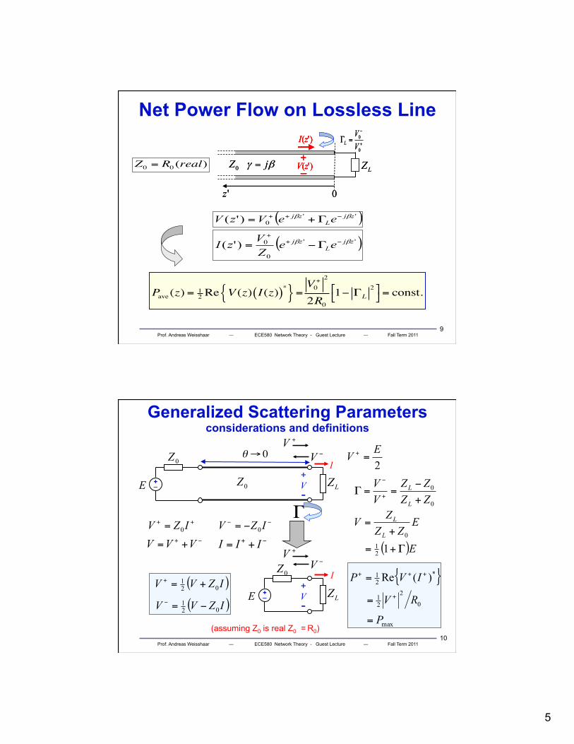
Transmission Line Basics
+ - V1
Port 1 Port 2
+ _ E1
Z0,1
+ _ E2
Z0,2
+1V
+2V
−2V
−1V
+ - V2 Z0, ! = "l
Lossless Transmission Line
V (z) =V0+e! j!z +V0
!e+ j!z
I(z) = I0+e! j!z + I0
!e+ j!z
Z0 =LC=V0
+
I0+= !
V0!
I0!
Characteristic Impedance:
! =" LCPhase Constant:
V2 =V2+ +V2
!
I2 = I2+ + I2
!
V1 =V1+ +V1
!
I1 = I1+ + I1
!
z0
5
Prof. Andreas Weisshaar ― ECE580 Network Theory - Guest Lecture ― Fall Term 2011 9
Net Power Flow on Lossless Line
Pave (z) = 12 Re V (z) I(z)( )*{ }=
V0+ 2
2R01! "L
2#$
%&= const.
( )''0)'( zj
Lzj eeVzV ββ −++ Γ+=
( )''
0
0)'( zjL
zj eeZVzI ββ −+
+
Γ−=
'z 0
LZβγ jZ =0
+
−
=Γ0
0
VV
L)'(zI
+–)'(zV
'z 0
LZβγ jZ =0
+
−
=Γ0
0
VV
L)'(zI )'(zI
+–)'(zV
+–)'(zVZ0 = R0 (real)
Prof. Andreas Weisshaar ― ECE580 Network Theory - Guest Lecture ― Fall Term 2011 10
Generalized Scattering Parameters considerations and definitions
I + _ E
0Z+
- V LZ0Z
+V−V
2EV =+
−+ += VVV −+ += III
++ = IZV 0−− −= IZV 0
( )IZVV 021 +=+
( )IZVV 021 −=−
0
0
ZZZZ
VV
L
L
+
−==Γ
+
−
( )E
EZZ
ZVL
L
Γ+=
+=
1210
{ }
max
0
2
21
*21 )(Re
P
RV
IVP
=
=
=
+
+++
+ _ E
0Z+
- V LZ
+V−VI
(assuming Z0 is real Z0 = R0)
!
!! 0
6
Prof. Andreas Weisshaar ― ECE580 Network Theory - Guest Lecture ― Fall Term 2011 11
Normalized Wave Quantities
+ _ E
0R+
- V LZ
ab
I
{ } 0
2
21*
21 )(Re RVIVP ++++ ==
§ It is useful to express power P without characteristic impedance (port impedance) Z0 = R0 (but P still depends on R0)
0RVa
+
=
{ } 0
2
21*
21 )(Re RVIVP −−−− =−=
0RVb
−
=
{ }2221
0
2
0
2
22
ba
RV
RV
PPPL
−=
−=−=−+
−+
(assuming real Z0)
Prof. Andreas Weisshaar ― ECE580 Network Theory - Guest Lecture ― Fall Term 2011 12
Scattering Matrix
⎥⎥⎥⎥
⎦
⎤
⎢⎢⎢⎢
⎣
⎡
⎥⎥⎥⎥
⎦
⎤
⎢⎢⎢⎢
⎣
⎡
=
⎥⎥⎥⎥
⎦
⎤
⎢⎢⎢⎢
⎣
⎡
NNNNN
N
N
a
aa
SSS
SSSSSS
b
bb
2
1
21
22221
11211
2
2
1
jkaj
iij
kabS
≠=
=for0
( ) ( ) )(22
allfor0,0
,0
allfor0,0
,0 jiRERV
RERV
SjkEjj
ii
jkEjj
iiij
kk
≠==
≠=≠=
−
+ - V1
I1
Port 1
Port 2
Port N
N-port Network
+ _ E1
R0,1
+ - V2
I2
+ _ E2
R0,2
+ - VN
IN
+ _ EN
R0,N
7
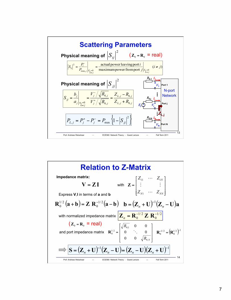
Prof. Andreas Weisshaar ― ECE580 Network Theory - Guest Lecture ― Fall Term 2011 13
Scattering Parameters
)(port frompowermaximumportleavingpoweractual
00max,
2ji
ji
PPS
jkE
jkEj
iij
kk
≠==≠=
≠=
−
Physical meaning of 2
ijS
Physical meaning of 2
jjS
jjL
jjL
jj
jj
jkaj
jjj RZ
RZRV
RVab
Sk ,0,
,0,
,0
,0
0 +
−===
+
−
≠=
{ }2max, 1 jjjjjL SPPPP −=−= −+
( = real) 00 RZ =
+-V1
I1
Port 1
Port j
Port N
N-portNetwork
R0,1
+-VjIj
+_Ej
R0,j
+-VN
INR0,NZL,j
+-V1
I1
Port 1
Port j
Port N
N-portNetwork
R0,1
+-VjIj
+_Ej
R0,j
+-VN
INR0,NZL,j
Prof. Andreas Weisshaar ― ECE580 Network Theory - Guest Lecture ― Fall Term 2011 14
Relation to Z-Matrix
IZV =
( ) ( )baRZbaR −=+ − 2/10
2/10
⎥⎥⎥
⎦
⎤
⎢⎢⎢
⎣
⎡
=
NR
R
,0
1,02/1
0
000000
R
( ) ( )aUZUZb −+= −nn
1
⎥⎥⎥
⎦
⎤
⎢⎢⎢
⎣
⎡
=
NNN
N
ZZ
ZZ
1
111
Z
( ) ( ) ( )( ) 11 −− +−=−+= UZUZUZUZS nnnn
2/10
2/10
−−= RZRZn
Impedance matrix:
with
Express V,I in terms of a and b
with normalized impedance matrix
and port impedance matrix ( ) 12/10
2/10
−− = RR
( = real) 00 RZ =

8
Prof. Andreas Weisshaar ― ECE580 Network Theory - Guest Lecture ― Fall Term 2011 15
Scattering Parameters
§ Port n is said to be matched when it is terminated with a load having the same impedance as the port impedance Z0,n.
§ Often, all port impedances are chosen to be equal and Z0,n = 50 Ω.
§ The values of the scattering (S-) parameters depend on the chosen port impedances.
§ S-parameters can be algebraically renormalized to different and unequal port impedances. (see later)
Prof. Andreas Weisshaar ― ECE580 Network Theory - Guest Lecture ― Fall Term 2011 16
Two-Port Networks Insertion and Return Loss
+ _ E
1,0Z
2,0Z⎥⎦
⎤⎢⎣
⎡
2221
1211
SSSS
RL IL Return Loss
indicates the extend of mismatch in a network in dB
dBinlog20 1110 SRL −=
Insertion Loss measure of transmitted fraction of power in dB
dBinlog20 2110 SIL −=
port 1:
from port 1 to port 2:
9
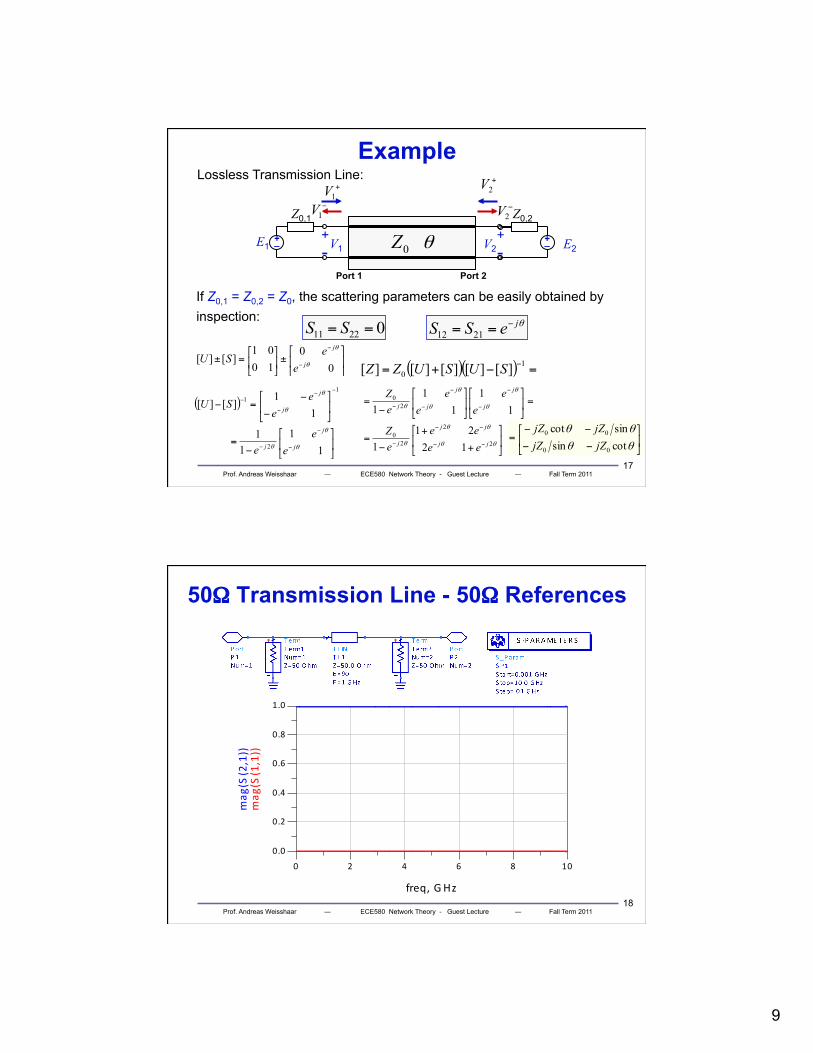
Prof. Andreas Weisshaar ― ECE580 Network Theory - Guest Lecture ― Fall Term 2011 17
Example
+ - V1
Port 1 Port 2
+ _ E1
Z0,1
+ _ E2
Z0,2
+1V
+2V
−2V
−1V
+ - V2 θ0Z
Lossless Transmission Line:
If Z0,1 = Z0,2 = Z0, the scattering parameters can be easily obtained by inspection:
02211 == SS θjeSS −== 2112
⎥⎦
⎤⎢⎣
⎡±⎥⎦
⎤⎢⎣
⎡=±
−
−
00
1001
][][θ
θ
j
j
ee
SU
( )
⎥⎦
⎤⎢⎣
⎡
−=
⎥⎦
⎤⎢⎣
⎡
−
−=−
−
−
−
−
−
−−
11
11
11
][][
2
11
θ
θ
θ
θ
θ
j
j
j
j
j
ee
e
ee
SU
( )( ) =−+= −10 ][][][][][ SUSUZZ
⎥⎦
⎤⎢⎣
⎡
+
+
−=
=⎥⎦
⎤⎢⎣
⎡⎥⎦
⎤⎢⎣
⎡
−=
−−
−−
−
−
−
−
−
−
θθ
θθ
θ
θ
θ
θ
θ
θ
2
2
20
20
1221
1
11
11
1
jj
jj
j
j
j
j
j
j
eeee
eZ
ee
ee
eZ
⎥⎦
⎤⎢⎣
⎡
−−
−−=
θθ
θθ
cotsinsincot
00
00
jZjZjZjZ
Prof. Andreas Weisshaar ― ECE580 Network Theory - Guest Lecture ― Fall Term 2011 18
50Ω Transmission Line - 50Ω References
2 4 6 80 10
0.2
0.4
0.6
0.8
0.0
1.0
freq, GHz
mag
(S(1,1))
mag
(S(2,1))

10
Prof. Andreas Weisshaar ― ECE580 Network Theory - Guest Lecture ― Fall Term 2011 19
50Ω Transmission Line - 100Ω References
2 4 6 80 10
0.2
0.4
0.6
0.8
0.0
1.0
freq, GHz
mag
(S(1,1))
mag
(S(2,1)) ( )
Ω=
Ω=
25100502inZ
6.01002510025
11 −=+
−=S
Prof. Andreas Weisshaar ― ECE580 Network Theory - Guest Lecture ― Fall Term 2011 20
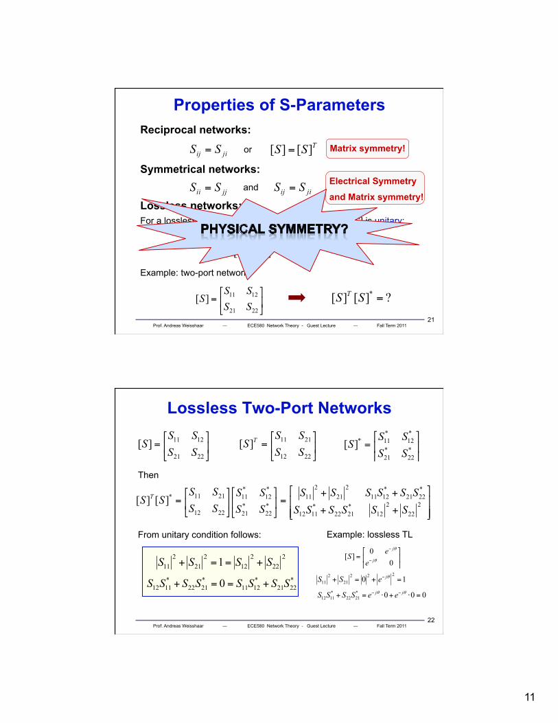
Properties of S-Parameters Reciprocal networks:
Symmetrical networks:
Lossless networks: For a lossless passive network the scattering matrix [S] is unitary:
jiij SS = TSS ][][ =
][][][ * USS T =
Matrix symmetry! or
jjii SS = jiij SS =and
transpose complex-conjugate
Example: two-port network
⎥⎦
⎤⎢⎣
⎡=
2221
1211][SSSS
S ?][][ * =SS T
Electrical Symmetry and Matrix symmetry!
11
Prof. Andreas Weisshaar ― ECE580 Network Theory - Guest Lecture ― Fall Term 2011 21
Properties of S-Parameters Reciprocal networks:
Symmetrical networks:
Lossless networks: For a lossless passive network the scattering matrix [S] is unitary:
jiij SS = TSS ][][ =
][][][ * USS T =
Matrix symmetry! or
jjii SS = jiij SS =and
transpose complex-conjugate
Example: two-port network
⎥⎦
⎤⎢⎣
⎡=
2221
1211][SSSS
S ?][][ * =SS T
Electrical Symmetry and Matrix symmetry!
Prof. Andreas Weisshaar ― ECE580 Network Theory - Guest Lecture ― Fall Term 2011 22
Lossless Two-Port Networks
⎥⎦
⎤⎢⎣
⎡=
2212
2111][SSSS
S T⎥⎦
⎤⎢⎣
⎡= *
22*21
*12
*11*][
SSSS
S
⎥⎥⎦
⎤
⎢⎢⎣
⎡
++
++=⎥
⎦
⎤⎢⎣
⎡⎥⎦
⎤⎢⎣
⎡= 2
222
12*2122
*1112
*2221
*1211
221
211
*22
*21
*12
*11
2212
2111*][][SSSSSSSSSSSS
SSSS
SSSS
SS T
⎥⎦
⎤⎢⎣
⎡=
2221
1211][SSSS
S
Then
From unitary condition follows:
222
212
221
211 1 SSSS +==+
*2221
*1211
*2122
*1112 0 SSSSSSSS +==+
Example: lossless TL
⎥⎦
⎤⎢⎣
⎡=
−
−
00
][θ
θ
j
j
ee
S
10222
212
11 =+=+ − θjeSS
000*2122
*1112 =⋅+⋅=+ −− θθ jj eeSSSS

12
Prof. Andreas Weisshaar ― ECE580 Network Theory - Guest Lecture ― Fall Term 2011 23
Lossless Two-Port Networks
⎥⎦
⎤⎢⎣
⎡=
2212
2111][SSSS
S T⎥⎦
⎤⎢⎣
⎡= *
22*21
*12
*11*][
SSSS
S
⎥⎥⎦
⎤
⎢⎢⎣
⎡
++
++=⎥
⎦
⎤⎢⎣
⎡⎥⎦
⎤⎢⎣
⎡= 2
222
12*2122
*1112
*2221
*1211
221
211
*22
*21
*12
*11
2212
2111*][][SSSSSSSSSSSS
SSSS
SSSS
SS T
⎥⎦
⎤⎢⎣
⎡=
2221
1211][SSSS
S
Then
From unitary condition follows:
222
212
221
211 1 SSSS +==+
*2221
*1211
*2122
*1112 0 SSSSSSSS +==+
≥≤1
for passive (lossy) networks
Prof. Andreas Weisshaar ― ECE580 Network Theory - Guest Lecture ― Fall Term 2011 24
Applications
+ _ E
SZ
LZ⎥⎦
⎤⎢⎣
⎡
2221
1211
SSSS
inΓ
port 1 refZ ,0port 2
Terminated Port:
one-port network
++− += 2121111 VSVSV++− += 2221212 VSVSV
+++ Γ+Γ= 2221212 VSVSV LL
−+ Γ= 22 VV LLΓ
++
Γ−
Γ= 1
22
212 1
VSSVL
L
22
211211 1 S
SSSL
Lin Γ−
Γ+=Γ
special case: ZL=0 è ΓL = -1
22
211211 1 S
SSSin +−=Γ
All port (reference) impedances are
(Zs = Z0,ref )

13
Prof. Andreas Weisshaar ― ECE580 Network Theory - Guest Lecture ― Fall Term 2011 25
Shift in Reference Plane
−− = AjB VeV 111θ
11 lΔ= βθ Two-PortNetwork[SB]0Z 0Z
AS11 AS22
AS21
AS12
shift in reference plane
shift in reference plane
A AB B1lΔ 2lΔ
+AV1+BV2−BV2−AV1
+BV1+AV2
−BV1−AV2
Two-PortNetwork[SB]0Z 0Z
AS11 AS22
AS21
AS12
shift in reference plane
shift in reference plane
A AB B1lΔ 2lΔ
+AV1+BV2−BV2−AV1
+BV1+AV2
−BV1−AV2
+−+ = AjB VeV 111θ
−− = AjB VeV 222θ
22 lΔ= βθ
+−+ = AjB VeV 222θ
⎥⎦
⎤⎢⎣
⎡⎥⎦
⎤⎢⎣
⎡⎥⎦
⎤⎢⎣
⎡=⎥
⎦
⎤⎢⎣
⎡⎥⎦
⎤⎢⎣
⎡+
+
−
−
−
−
B
B
j
j
AA
AA
B
B
j
j
VV
ee
SSSS
VV
ee
2
1
2221
1211
2
12
1
2
1
00
00
θ
θ
θ
θ
⎥⎦
⎤⎢⎣
⎡⎥⎦
⎤⎢⎣
⎡⎥⎦
⎤⎢⎣
⎡=⎥⎦
⎤⎢⎣
⎡2
1
2
1
00
00
2221
1211
2221
1211θ
θ
θ
θ
j
j
AA
AA
j
j
BB
BB
ee
SSSS
ee
SSSS
Prof. Andreas Weisshaar ― ECE580 Network Theory - Guest Lecture ― Fall Term 2011 26
S-Matrix Renormalization
( ) ( ) ( )( ) 11 −− +−=−+= UZUZUZUZS nnnn
( )( ) 1−−+= SUSUZn
FZFRZRZ old2/1new,0
2/1new,0
newnn == −−
⎥⎥⎥⎥
⎦
⎤
⎢⎢⎢⎢
⎣
⎡
=new,0
old,0
new1,0
old1,0
000000
NN RR
RRF
Renormalization matrix ( = real) 00 RZ =

14
Prof. Andreas Weisshaar ― ECE580 Network Theory - Guest Lecture ― Fall Term 2011 27
0.1 0.2 0.4 0.5 0.6 0.8 1 2 4 8 16 32
j0.25
-j0.25
0
j0.5
-j0.5
0
j0.75
-j0.75
0
j1
-j1
0
j1.5
-j1.5
0
j2
-j2
0
j2.5
-j2.5
0
j3
-j3
0
j4
-j4
0
j5
-j5
0
Measurement Initial ECM Perturbed & Augmented ECM
S11
S21
S22
S22
Example
125Ω
Circuit Model
155Ω
Prof. Andreas Weisshaar ― ECE580 Network Theory - Guest Lecture ― Fall Term 2011 28
Comparison of Different Port Normalizations
Ω=Ω= 155125 2,01,0 ZZ Ω== 502,01,0 ZZ
S11
15
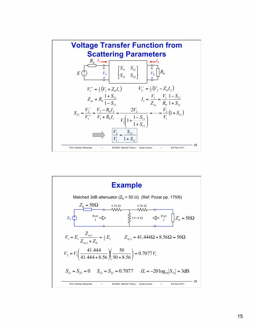
Prof. Andreas Weisshaar ― ECE580 Network Theory - Guest Lecture ― Fall Term 2011 29
Voltage Transfer Function from Scattering Parameters
+ _ E
0R
0R⎥⎦
⎤⎢⎣
⎡
2221
1211
SSSS
( )10121
1 IZVV +=+ ( )20221
2 IZVV −=−
11
11
0
111 1
1SS
RV
ZVIin +
−==
11
110 11SSRZin −
+=
+
- V1
+
- V2
( )111
2
11
111
2
101
202
1
221 1
111
2 SVV
SSV
VIRVIRV
VVS +==
⎟⎟⎠
⎞⎜⎜⎝
⎛
+−
+
=+
−==
+
−
11
21
1
2
1 SS
VV
+=
I1 I2
Prof. Andreas Weisshaar ― ECE580 Network Theory - Guest Lecture ― Fall Term 2011 30
Example Matched 3dB attenuator (Z0 = 50 Ω) (Ref: Pozar pp. 175/6)
Ω= 500Z+ _ E1
Ω= 500Z
121
01,
1,11 E
ZZZ
EVin
in =+
=
112 7077.056.850
5056.8444.41
444.41 VVV =⎟⎠
⎞⎜⎝
⎛+
⎟⎠
⎞⎜⎝
⎛+
=
02211 == SS
Ω≈Ω+Ω= 5056.8444.411,inZ
7077.02112 == SS dB3log20 2110 =−= SIL

16
Prof. Andreas Weisshaar ― ECE580 Network Theory - Guest Lecture ― Fall Term 2011 31
Example using Z-Matrix
Ω= 500Z+ _ E1
Ω= 500Z
Ω⎥⎦
⎤⎢⎣
⎡=
36.15080.14180.14136.150
Z
⎥⎦
⎤⎢⎣
⎡== −−
0072.38360.28360.20072.32/1
02/1
0 RZRZn ⎥⎦
⎤⎢⎣
⎡=
07077.07077.00
S
⎥⎦
⎤⎢⎣
⎡== −−
5036.10054.20054.20072.32/1
02/1
0 RZRZn ⎥⎦
⎤⎢⎣
⎡
−=
3333.06672.06672.01670.0
S
Ω== 502,01,0 ZZ
Ω=Ω= 10050 2,01,0 ZZ
Prof. Andreas Weisshaar ― ECE580 Network Theory - Guest Lecture ― Fall Term 2011 32
Example using Z-Matrix
Ω= 500Z+ _ E1
Ω= 500Z
Ω⎥⎦
⎤⎢⎣
⎡=
36.15080.14180.14136.150
Z
⎥⎦
⎤⎢⎣
⎡== −−
0072.38360.28360.20072.32/1
02/1
0 RZRZn ⎥⎦
⎤⎢⎣
⎡=
07077.07077.00
S
⎥⎦
⎤⎢⎣
⎡== −−
5036.10054.20054.20072.32/1
02/1
0 RZRZn ⎥⎦
⎤⎢⎣
⎡
−=
3333.06672.06672.01670.0
S
Ω== 502,01,0 ZZ
Ω=Ω= 10050 2,01,0 ZZ
Attenuator terminated in ZL=100Ω and S-Parameters wrt Z0,1=Z0,2=50Ω
167.021
21
31
1 211222
211211 ==Γ=
Γ−
Γ+=Γ SS
SSSS LL
Lin
Attenuator terminated in ZL=100Ω and S-Parameters wrt Z0,1=50Ω Z0,2=100Ω
167.01 11
22
211211 ==
Γ−
Γ+=Γ S
SSSSL
Lin
31
5010050100
2,0
2,0 =+
−=
+
−=Γ
ZZZZ
L
LL
02,0
2,0 =+
−=Γ
ZZZZ
L
LL
17
Prof. Andreas Weisshaar ― ECE580 Network Theory - Guest Lecture ― Fall Term 2011 33
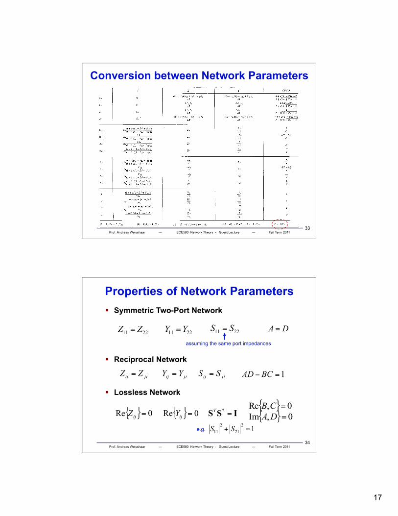
Conversion between Network Parameters
Prof. Andreas Weisshaar ― ECE580 Network Theory - Guest Lecture ― Fall Term 2011 34
Properties of Network Parameters § Symmetric Two-Port Network
§ Reciprocal Network
§ Lossless Network
jiij ZZ = jiij YY = jiij SS = 1=− BCAD
2211 ZZ = 2211 YY = DA =2211 SS =
assuming the same port impedances
{ } 0Re =ijZ ISS =*T{ } 0Re =ijY
1221
211 =+ SSe.g.
{ } 0,Re =CB{ } 0,Im =DA