eﬃcient experimental design with marketing research...

Efficient Experimental Design

with Marketing Research Applications

Warren F. Kuhfeld

Randall D. Tobias

Mark Garratt

Abstract

We suggest using D-efficient experimental designs for conjoint and discrete-choice studies, and discussorthogonal arrays, nonorthogonal designs, relative efficiency, and nonorthogonal design algorithms. Weconstruct designs for a choice study with asymmetry and interactions and for a conjoint study withblocks and aggregate interactions.∗

Introduction

The design of experiments is a fundamental part of marketing research. Experimental designs arerequired in widely used techniques such as preference-based conjoint analysis and discrete-choice studies(e.g., Carmone and Green 1981; Elrod, Louviere, and Davey 1992; Green and Wind 1975; Huber, et al.1993; Lazari and Anderson 1994; Louviere 1991; Louviere and Woodworth 1983; Wittink and Cattin1989). Ideally, marketing researchers prefer orthogonal designs. When a linear model is fit with anorthogonal design, the parameter estimates are uncorrelated, which means each estimate is independentof the other terms in the model. More importantly, orthogonality usually implies that the coefficientswill have minimum variance, though we discuss exceptions to this rule. For these reasons, orthogonaldesigns are usually quite good. However, for many practical problems, orthogonal designs are simplynot available. In those situations, nonorthogonal designs must be used.

∗This chapter is a revision of a paper that appeared in Journal of Marketing Research, November, 1994, pages 545–557.Warren F. Kuhfeld is now Manager, Multivariate Models R&D, SAS. Randall D. Tobias is now Manager, Linear ModelsR&D, SAS. Mark Garratt was Vice President, Conway | Milliken & Associates when this paper was first published in1994 and is now with Miller Brewing Company. The authors thank Jordan Louviere, JMR editor Barton Weitz, and threeanonymous reviewers for their helpful comments on earlier versions of this article. Thanks to Michael Ford for the ideafor the second example. The JMR article was based on a presentation given to the AMA Advanced Research TechniquesForum, June 14, 1993, Monterey CA.

Our primary message when this paper was published in 1994 was that marketing researchers should use D-efficientexperimental designs. This message remains as strong as ever, but today, we have much better tools for accomplishingthis than we had in 1994. Most of the revisions of the original paper are due to improvements in the tools. Ournew design tool, the %MktEx SAS macro, is easier to use than our old tools, and it usually makes better designs.Copies of this chapter (MR-2010D), the other chapters, sample code, and all of the macros are available on the Webhttp://support.sas.com/resources/papers/tnote/tnote_marketresearch.html.

243

244 MR-2010D — Efficient Experimental Design with Marketing Research Applications

Orthogonal designs are available for only a relatively small number of very specific problems. Theymay not be available when some combinations of factor levels are infeasible, a nonstandard number ofruns (factor level combinations or hypothetical products) is desired, or a nonstandard model is beingused, such as a model with interaction or polynomial effects. Consider the problem of designing adiscrete choice study in which there are alternative specific factors, different numbers of levels withineach factor, and interactions within each alternative. Orthogonal designs are not readily available forthis situation, particularly when the number of runs must be limited. When an orthogonal designis not available, an alternative must be chosen—the experiment can be modified to fit some knownorthogonal design, which is undesirable for obvious reasons, or a known design can be modified to fitthe experiment, which may be difficult and inefficient.

Our primary purpose is to explore a third alternative, the use of optimal (or nearly optimal) designs.Such designs are typically nonorthogonal; however they are efficient in the sense that the variances andcovariances of the parameter estimates are minimized. Furthermore, they are always available, even fornonstandard situations. Finding these designs usually requires the aid of a computer, but we want toemphasize that we are not advocating a black-box approach to designing experiments. Computerizeddesign algorithms do not supplant traditional design-creation skills. Our examples show that our bestdesigns were usually found when we used our human design skills to guide the computerized search.

First, we will summarize our main points; next, we will review some fundamentals of the designof experiments; then we will discuss computer-generated designs, a discrete-choice example, and aconjoint analysis example.

Summary of Main Points. Our goal is to explain the benefits of using computer-generated designsin marketing research. Our main points follow:

1. The goodness of an experimental design (efficiency) can be quantified as a function of the vari-ances and covariances of the parameter estimates. Efficiency increases as the variances decrease.Designs should not be thought of in terms of the dichotomy between orthogonal versus nonorthog-onal but rather as varying along the continuous attribute of efficiency. Some orthogonal designsare less efficient than other (orthogonal and nonorthogonal) alternatives.

2. Orthogonality is not the primary goal in design creation. It is a secondary goal, associated withthe primary goal of minimizing the variances of the parameter estimates. Degree of orthogonalityis an important consideration, but other factors should not be ignored.

3. For complex, nonstandard situations, computerized searches provide the only practical methodof design generation for all but the most sophisticated of human designers. These situations donot have to be avoided just because it is extremely difficult to generate a good design manually.

4. The best approach to design creation is to use the computer as a tool along with traditionaldesign skills, not as a substitute for thinking about the problem.

Background and Assumptions. We present an overview of the theory of efficient experimentaldesign, developed for the general linear model. This topic is well known to specialists in statisticalexperimentation, though it is not typically taught in design classes. Then we will suggest ways in whichthis theory can be applied to marketing research problems.

MR-2010D — Efficient Experimental Design with Marketing Research Applications 245

Certain assumptions must be made before applying ordinary general linear model theory to problems inmarketing research. The usual goals in linear modeling are to estimate parameters and test hypothesesabout those parameters. Typically, independence and normality are assumed. In conjoint analysis, eachsubject rates all products and separate ordinary-least-squares analyses are run for each subject. Thisis not a standard general linear model; in particular, observations are not independent and normalitycannot be assumed. Discrete choice models, which are nonlinear, are even further removed from thegeneral linear model.

Marketing researchers have always made the critical assumption that designs that are good for generallinear models are also good for conjoint analysis and discrete choice. We also make this assumption.Specifically, we assume the following:

1. Market share estimates computed from a conjoint analysis model using a more efficient designwill be better than estimates using a less efficient design. That is, more efficient designs meanbetter estimates of the part-worth utilities, which lead to better estimates of product utility andmarket share.

2. An efficient design for a linear model is a good design for the multinomial logit (MNL) modelused in discrete choice studies.

Investigating these standard assumptions is beyond the scope of this article. However, they are sup-ported by Carson and colleagues (1994), our experiences in consumer product goods, and limitedsimulation results. Much more research is needed on this topic, particularly in the area of discretechoice.

Design of Experiments

Orthogonal Experimental Designs. An experimental design is a plan for running an experiment.The factors of an experimental design are variables that have two or more fixed values, or levels.Experiments are performed to study the effects of the factor levels on the dependent variable. In aconjoint or discrete-choice study, the factors are the attributes of the hypothetical products or services,and the response is preference or choice.

A simple experimental design is the full-factorial design, which consists of all possible combinationsof the levels of the factors. For example, with five factors, two at two levels and three at three levels(denoted 2233), there are 108 possible combinations. In a full-factorial design, all main effects, two-way interactions, and higher-order interactions are estimable and uncorrelated. The problem witha full-factorial design is that, for most practical situations, it is too cost-prohibitive and tedious tohave subjects rate all possible combinations. For this reason, researchers often use fractional-factorialdesigns, which have fewer runs than full-factorial designs. The price of having fewer runs is that someeffects become confounded. Two effects are confounded or aliased when they are not distinguishablefrom each other.

A special type of fractional-factorial design is the orthogonal array, in which all estimable effects areuncorrelated. Orthogonal arrays are categorized by their resolution. The resolution identifies whicheffects, possibly including interactions, are estimable. For example, for resolution III designs, all maineffects are estimable free of each other, but some of them are confounded with two-factor interactions.


For resolution V designs, all main effects and two-factor interactions are estimable free of each other.Higher resolutions require larger designs. Orthogonal arrays come in specific numbers of runs (e.g., 16,18, 20, 24, 27, 28) for specific numbers of factors with specific numbers of levels.

Resolution III orthogonal arrays are frequently used in marketing research. The term “orthogonalarray,” as it is sometimes used in practice, is imprecise. It correctly refers to designs that are bothorthogonal and balanced, and hence optimal. It is also imprecisely used to refer to designs thatare orthogonal but not balanced, and hence potentially nonoptimal. A design is balanced when eachlevel occurs equally often within each factor, which means the intercept is orthogonal to each effect.Imbalance is a generalized form of nonorthogonality, which increases the variances of the parameterestimates.

Design Efficiency. Efficiencies are measures of design goodness. Common measures of theefficiency of an (ND × p) design matrix X are based on the information matrix X′X. The variance-covariance matrix of the vector of parameter estimates β in a least-squares analysis is proportionalto (X′X)−1. An efficient design will have a “small” variance matrix, and the eigenvalues of (X′X)−1

provide measures of its “size.” Two common efficiency measures are based on the idea of “averageeigenvalue” or “average variance.” A-efficiency is a function of the arithmetic mean of the eigenvalues,which is given by trace ((X′X)−1)/p. D-efficiency is a function of the geometric mean of the eigenvalues,which is given by |(X′X)−1|1/p. A third common efficiency measure, G-efficiency, is based on σM , themaximum standard error for prediction over the candidate set. All three of these criteria are convexfunctions of the eigenvalues of (X′X)−1 and hence are usually highly correlated.

For all three criteria, if a balanced and orthogonal design exists, then it has optimum efficiency;conversely, the more efficient a design is, the more it tends toward balance and orthogonality. A designis balanced and orthogonal when (X′X)−1 is diagonal (for a suitably coded X, see page 73). A design isorthogonal when the submatrix of (X′X)−1, excluding the row and column for the intercept, is diagonal;there may be off-diagonal nonzeros for the intercept. A design is balanced when all off-diagonal elementsin the intercept row and column are zero.

These measures of efficiency can be scaled to range from 0 to 100 (for a suitably coded X):

A-efficiency = 100× 1ND trace ((X′X)−1)/p

D-efficiency = 100× 1ND |(X′X)−1|1/p

G-efficiency = 100×√

p/ND

σM

These efficiencies measure the goodness of the design relative to hypothetical orthogonal designs thatmay be far from possible, so they are not useful as absolute measures of design efficiency. Instead, theyshould be used relatively, to compare one design with another for the same situation. Efficiencies thatare not near 100 may be perfectly satisfactory.

Figure 1 shows an optimal design in four runs for a simple example with two factors, using interval-measure scales for both. There are three candidate levels for each factor. The full-factorial design isshown by the nine asterisks, with circles around the optimal four design points. As this example shows,


Figure 1Candidate Set and Optimal Design

-1

0

1

-1 0 1

Two 3-Level Factors

*

* * *

*

* - Candidate Point

- Optimal Design Point

**

* *

*

Table 1Full-Factorial Design

Information Matrix

Int X1 X2 X3 - X4 - X5 -

Int 108 0 0 0 0 0 0 0 0X1 0 108 0 0 0 0 0 0 0X2 0 0 108 0 0 0 0 0 0X3 0 0 0 108 0 0 0 0 0

- 0 0 0 0 108 0 0 0 0X4 0 0 0 0 0 108 0 0 0

- 0 0 0 0 0 0 108 0 0X5 0 0 0 0 0 0 0 108 0

- 0 0 0 0 0 0 0 0 108

100.0000 D-efficiency100.0000 A-efficiency100.0000 G-efficiency

efficiency tends to emphasize the corners of the design space. Interestingly, nine different sets of fourpoints form orthogonal designs—every set of four that forms a rectangle or square. Only one of theseorthogonal designs is optimal, the one in which the points are spread out as far as possible.

Computer-Generated Design Algorithms. When a suitable orthogonal design does not exist, computer-generated nonorthogonal designs can be used instead. Various algorithms exist for selecting a good setof design points from a set of candidate points. The candidate points consist of all of the factor-levelcombinations that can potentially be included in the design—for example the nine points in Figure1. The number of runs, ND, is chosen by the researcher. Unlike orthogonal arrays, ND can be anynumber as long as ND ≥ p.† The algorithm searches the candidate points for a set of ND design pointsthat is optimal in terms of a given efficiency criterion.

It is almost never possible to list all ND-run designs and choose the most efficient or optimal design,because run time is exponential in the number of candidates. For example, with 2233 in 18 runs, thereare 108!/(18!(108− 18)!) = 1.39× 1020 possible designs. Instead, nonexhaustive search algorithms areused to generate a small number of designs, and the most efficient one is chosen. The algorithms selectpoints for possible inclusion or deletion, then compute rank-one or rank-two updates of some efficiencycriterion. The points that most increase efficiency are added to the design. These algorithms invariablyfind efficient designs, but they may fail to find the optimal design, even for the given criterion. Forthis reason, we prefer to use terms like information-efficient and D-efficiency over the more commonoptimal and D-optimal.

There are many algorithms for generating information-efficient designs. We will begin by describingsome of the simpler approaches and then proceed to the more complicated (and more reliable) algo-

†In fact, this restriction is not strictly necessary. So called “super-saturated” designs (Booth and Cox 1962) have moreruns than parameters. However, such designs are typically not used in marketing research. The %MktRuns SAS macroprovides some guidance on the selection of ND. See page 1159.


rithms. Dykstra’s (1971) sequential search method starts with an empty design and adds candidatepoints so that the chosen efficiency criterion is maximized at each step. This algorithm is fast, but itis not very reliable in finding a globally optimal design. Also, it always finds the same design (due toa lack of randomness).

The Mitchell and Miller (1970) simple exchange algorithm is a slower but more reliable method. Itimproves the initial design by adding a candidate point and then deleting one of the design points,stopping when the chosen criterion ceases to improve. The DETMAX algorithm of Mitchell (1974)generalizes the simple exchange method. Instead of following each addition of a point by a deletion,the algorithm makes excursions in which the size of the design may vary. These three algorithms addand delete points one at a time.

The next two algorithms add and delete points simultaneously, and for this reason, are usually morereliable for finding the truly optimal design; but because each step involves a search over all possiblepairs of candidate and design points, they generally run much more slowly (by an order of magnitude).The Fedorov (1972) algorithm simultaneously adds one candidate point and deletes one design point.Cook and Nachtsheim (1980) define a modified Fedorov algorithm that finds the best candidate pointto switch with each design point. The resulting procedure is generally as efficient as the simple Fedorovalgorithm in finding the optimal design, but it is up to twice as fast. We extensively use one morealgorithm, the coordinate exchange algorithm of Meyer and Nachtsheim (1995). This algorithm doesnot use a candidate set. Instead it refines an initial design by exchanging each level with every otherpossible level, keeping those exchanges that increase efficiency. In effect, this method uses a virtualcandidate set that consists of all possible runs, even when the full-factorial candidate set is too largeto generate and store.

Choice of Criterion and Algorithm. Typically, the choice of efficiency criterion is less importantthan the choice between manual design creation and computerized search. All of the information-efficient designs presented in this article were generated optimizing D-efficiency because it is faster tooptimize than A-efficiency and because it is the standard approach. It is also possible to optimizeA-efficiency, though the algorithms generally run much more slowly because the rank-one updatesare more complicated with A-efficiency. G-efficiency is an interesting ancillary statistic; however, ourexperience suggests that attempts to maximize G-efficiency with standard algorithms do not work verywell.

The candidate set search algorithms, ordered from the fastest and least reliable to the slowest andmost reliable, are: sequential, simple exchange, DETMAX, and modified Fedorov. We always use themodified Fedorov and coordinate exchange algorithms even for extremely large problems; we nevereven try the other algorithms. For small problems in which the full factorial is no more than a fewthousand runs, modified Fedorov tends to work best. For larger problems, coordinate exchange tendsto be better. Our latest software, the %MktEx macro, tries a few iterations with both methods, thenpicks the best method for that problem and continues on with more iterations using just the chosenmethod. See page 1017 and all of the examples starting on page 285.

Nonlinear Models. The experimental design problem is relatively simple for linear models and muchmore complicated for nonlinear models. The usual goal when creating a design is to minimize somefunction of the variance matrix of the parameter estimates, such as the determinant. For linear models,the variance matrix is proportional to (X′X)−1, and so the design optimality problem is well-posed.However, for nonlinear models, such as the multinomial logit model used with discrete-choice data, thevariance matrix depends on the true values of the parameters themselves. (See pages 265, 806, and


556 for more on efficient choice designs based on assumptions about the parameters.) Thus in general,there may not exist a design for a discrete-choice experiment that is always optimal. However, Carsonand colleagues (1994) and our experience suggest that D-efficient designs work well for discrete-choicemodels.

Lazari and Anderson (1994) provide a catalog of designs for discrete-choice models, which are goodfor certain specific problems. For those specific situations, they may be as good as or better thancomputer-generated designs. However, for many real problems, cataloged designs cannot be usedwithout modification, and modification can reduce efficiency. We carry their work one step further bydiscussing a general computerized approach to design generation.

Design Comparisons

Comparing Orthogonal Designs. All orthogonal designs are not perfectly or even equally efficient. Inthis section, we compare designs for 2233. Table 1 gives the information matrix, X′X, for a full-factorialdesign using an orthogonal coding. The matrix is a diagonal matrix with the number of runs on thediagonal. The three efficiency criteria are displayed after the information matrix. Because this is afull-factorial design, all three criteria show that the design is 100% efficient. The variance matrix (notshown) is (1/108)I = 0.0093I.

Table 2 shows the information matrix, efficiencies, and variance matrix for a classical 18-run orthogonaldesign for 2233, Chakravarti’s (1956) L18, for comparison with information-efficient designs with 18runs. (The SAS ADX menu system was used to generate the design. Tables A1 and A2 contain thefactor levels and the orthogonal coding used in generating Table 2.) Note that although the factors areall orthogonal to each other, X1 is not balanced. Because of this, the main effect of X1 is estimatedwith a higher variance (0.063) than X2 (0.056).

The precision of the estimates of the parameters critically depends on the efficiency of the experimentaldesign. The parameter estimates in a general linear model are always unbiased (in fact, best linearunbiased [BLUE]) no matter what design is chosen. However, all designs are not equally efficient. Infact, all orthogonal designs are not equally efficient, even when they have the same factors and thesame number of runs. Efficiency criteria can be used to help choose among orthogonal designs. Forexample, the orthogonal design in Tables 3 and A3 (from the Green and Wind 1975 carpet cleanerexample) for 2233 is less D-efficient than the Chakravarti L18 (97.4166/98.6998 = 0.9870). The Greenand Wind design can be created from a 35 balanced orthogonal array by collapsing two of the three-level factors into two-level factors. In contrast, the Chakravarti design is created from a 2134 balancedorthogonal array by collapsing only one of the three-level factors into a two-level factor. The extraimbalance makes the Green and Wind design less efficient. (Note that the off-diagonal 2 in the Greenand Wind information matrix does not imply that X1 and X2 are correlated. It is an artifact of thecoding scheme. The off-diagonal 0 in the variance matrix shows that X1 and X2 are uncorrelated.)

Orthogonal Versus Nonorthogonal Designs. Orthogonal designs are not always more efficient thannonorthogonal designs. Tables 4 and A4 show the results for an information-efficient, main-effects-onlydesign in 18 runs. The OPTEX procedure of SAS software was used to generate the design, using themodified Fedorov algorithm. The information-efficient design is slightly better than the classical L18,in terms of the three efficiency criteria. In particular, the ratio of the D-efficiencies for the classicaland information-efficient designs are 99.8621/98.6998 = 1.0118. In contrast to the L18, this design is


Table 2Orthogonal DesignInformation Matrix

Int X1 X2 X3 - X4 - X5 -

Int 18 6 0 0 0 0 0 0 0X1 6 18 0 0 0 0 0 0 0X2 0 0 18 0 0 0 0 0 0X3 0 0 0 18 0 0 0 0 0

- 0 0 0 0 18 0 0 0 0X4 0 0 0 0 0 18 0 0 0

- 0 0 0 0 0 0 18 0 0X5 0 0 0 0 0 0 0 18 0

- 0 0 0 0 0 0 0 0 18


Variance Matrix

Int X1 X2 X3 - X4 - X5 -

Int 63 -21 0 0 0 0 0 0 0X1 -21 63 0 0 0 0 0 0 0X2 0 0 56 0 0 0 0 0 0X3 0 0 0 56 0 0 0 0 0

- 0 0 0 0 56 0 0 0 0X4 0 0 0 0 0 56 0 0 0

- 0 0 0 0 0 0 56 0 0X5 0 0 0 0 0 0 0 56 0

- 0 0 0 0 0 0 0 0 56

Note: multiply variance matrix values by 0.001.

Table 3Green & Wind Orthogonal Design

Information Matrix

Int X1 X2 X3 - X4 - X5 -

Int 18 -6 -6 0 0 0 0 0 0X1 -6 18 2 0 0 0 0 0 0X2 -6 2 18 0 0 0 0 0 0X3 0 0 0 18 0 0 0 0 0

- 0 0 0 0 18 0 0 0 0X4 0 0 0 0 0 18 0 0 0

- 0 0 0 0 0 0 18 0 0X5 0 0 0 0 0 0 0 18 0

- 0 0 0 0 0 0 0 0 18


Variance Matrix

Int X1 X2 X3 - X4 - X5 -

Int 69 21 21 0 0 0 0 0 0X1 21 63 0 0 0 0 0 0 0X2 21 0 63 0 0 0 0 0 0X3 0 0 0 56 0 0 0 0 0

- 0 0 0 0 56 0 0 0 0X4 0 0 0 0 0 56 0 0 0

- 0 0 0 0 0 0 56 0 0X5 0 0 0 0 0 0 0 56 0

- 0 0 0 0 0 0 0 0 56

Notes: multiply variance matrix values by 0.001.

balanced in all the factors, but X1 and X2 are slightly correlated, shown by the 2’s off the diagonal.There is no completely orthogonal (that is, both balanced and orthogonal) 2233 design in 18 runs.‡ Thenonorthogonality in Table 4 has a much smaller effect on the variances of X1 and X2 (1.2%) than thelack of balance in the orthogonal design in Table 2 has on the variance of X2 (12.5%). In optimizingefficiency, the search algorithms effectively optimize both balance and orthogonality. In contrast, insome orthogonal designs, balance and efficiency may be sacrificed to preserve orthogonality.

This example shows that a nonorthogonal design may be more efficient than an unbalanced orthogonaldesign. We have seen this phenomenon with other orthogonal designs and in other situations as well.Preserving orthogonality at all costs can lead to decreased efficiency. Orthogonality was extremelyimportant in the days before general linear model software became widely available. Today, it is moreimportant to consider efficiency when choosing a design. These comparisons are interesting because theyillustrate in a simple example how lack of orthogonality and imbalance affect efficiency. Nonorthogonaldesigns will never be more efficient than balanced orthogonal designs, when they exist. However,nonorthogonal designs may well be more efficient than unbalanced orthogonal designs. Although thispoint is interesting and important, what is most important is that good nonorthogonal designs exist in

‡In order for the design to be both balanced and orthogonal, the number of runs must be divisible by 2, 3, 2 × 2,3 × 3, and 2 × 3. Since 18 is not divisible by 2 × 2, orthogonality and balance are not both simultaneously possible forthis design.


Table 4Information-Efficient Orthogonal Design

Information Matrix

Int X1 X2 X3 - X4 - X5 -

Int 18 0 0 0 0 0 0 0 0X1 0 18 2 0 0 0 0 0 0X2 0 2 18 0 0 0 0 0 0X3 0 0 0 18 0 0 0 0 0

- 0 0 0 0 18 0 0 0 0X4 0 0 0 0 0 18 0 0 0

- 0 0 0 0 0 0 18 0 0X5 0 0 0 0 0 0 0 18 0

- 0 0 0 0 0 0 0 0 18


Variance Matrix

Int X1 X2 X3 - X4 - X5 -

Int 56 0 0 0 0 0 0 0 0X1 0 56 -6 0 0 0 0 0 0X2 0 -6 56 0 0 0 0 0 0X3 0 0 0 56 0 0 0 0 0

- 0 0 0 0 56 0 0 0 0X4 0 0 0 0 0 56 0 0 0

- 0 0 0 0 0 0 56 0 0X5 0 0 0 0 0 0 0 56 0

- 0 0 0 0 0 0 0 0 56

Notes: multiply variance matrix values by 0.001.The diagonal entries for X1 and X2 are slightly largerat 0.0563 than the other diagonal entries of 0.0556.

Table 5Unrealistic Combinations Excluded

Information Matrix

Int X1 X2 X3 - X4 - X5 -

Int 18 0 0 0 0 0 0 0 0X1 0 18 2 0 0 0 0 0 0X2 0 2 18 0 0 0 0 0 0X3 0 0 0 18 0 0 0 0 0

- 0 0 0 0 18 0 0 0 0X4 0 0 0 0 0 18 0 -6 5

- 0 0 0 0 0 0 18 5 0X5 0 0 0 0 0 -6 5 18 0

- 0 0 0 0 0 5 0 0 18


Variance Matrix

Int X1 X2 X3 - X4 - X5 -

Int 56 0 0 0 0 0 0 0 0X1 0 56 -6 0 0 0 0 0 0X2 0 -6 56 0 0 0 0 0 0X3 0 0 0 56 0 0 0 0 0

- 0 0 0 0 56 0 0 0 0X4 0 0 0 0 0 69 -7 25 -20

- 0 0 0 0 0 -7 61 -20 2X5 0 0 0 0 0 25 -20 69 -7

- 0 0 0 0 0 -20 2 -7 61

Notes: multiply variance matrix values by 0.001.

many situations in which no orthogonal designs exist. These designs are also discussed and at a morebasic level starting on page 63.

Design Considerations

Codings and Efficiency. The specific design matrix coding does not affect the relative D-efficiency of competing designs. Rank-preserving linear transformations are immaterial, whether theyare from full-rank indicator variables to effects coding or to an orthogonal coding such as the oneshown in Table A2. Any full-rank coding is equivalent to any other. The absolute D-efficiency valueswill change, but the ratio of two D-efficiencies for competing designs is constant. Similarly, scale forquantitative factors does not affect relative efficiency. The proof is simple. If design X1 is recodedto X1A, then |(X1A)′(X1A)| = |A′X′

1X1A| = |AA′||X′1X1|. The relative efficiency of design X1

compared to X2 is the same as X1A compared to X2A, since the |AA′|’s terms in efficiency ratios


will cancel. We prefer the orthogonal coding because it yields “nicer” information matrices with thenumber of runs on the diagonal and efficiency values scaled so that 100 means perfect efficiency.

Quantitative Factors. The factors in an experimental design are usually qualitative (nominal), butquantitative factors such as price are also important. With quantitative factors, the choice of levelsdepends on the function of the original variable that is modeled. To illustrate, consider a pricing studyin which price ranges from $0.99 to $1.99. If a linear function of price is modeled, only two levelsof price should be used—the end points ($0.99 and $1.99). Using prices that are closer together isinefficient; the variances of the estimated coefficients will be larger. The efficiency of a given design isaffected by the coding of quantitative factors, even though the relative efficiency of competing designsis unaffected by coding. Consider treating the second factor of the Chakravarti L18, 2233 as linear.It is nearly three times more D-efficient to use $0.99 and $1.99 as levels instead of $1.49 and $1.50(58.6652/21.0832 = 2.7826). To visualize this, imagine supporting a yard stick (line) on your two indexfingers (with two points). The effect on the slope of the yard stick of small vertical changes in fingerlocations is much greater when your fingers are closer together than when they are near the ends.

Of course there are other considerations besides the numerical measure of efficiency. It would not makesense to use prices of $0.01 and $1,000,000 just because that is more efficient than using $0.99 and$1.99. The model is almost certainly not linear over this range. To maximize efficiency, the rangeof experimentation for quantitative factors should be as large as possible, given that the model isplausible.

The number of levels also affects efficiency. Because two points define a line, it is inefficient to use morethan two points to model a linear function. When a quadratic function is used (x and x2 are includedin the model), three points are needed—the two extremes and the midpoint. Similarly, four points areneeded for a cubic function. More levels are needed when the functional form is unknown. Extra levelsallow for the examination of complicated nonlinear functions, with a cost of decreased efficiency forthe simpler functions. When the function is assumed to be linear, experimental points should not bespread throughout the range of experimentation. See page 1213 for a discussion of nonlinear functionsof quantitative factors in conjoint analysis.

Most of the discussion outside this section has concerned qualitative (nominal) factors, even if thatwas not always explicitly stated. Quantitative factors complicate general design characterizations. Forexample, we previously stated that “if a balanced and orthogonal design exists, then it has optimumefficiency.” This statement must be qualified to be absolutely correct. The design would not be optimalif, for example, a three-level factor were treated as quantitative and linear.

Nonstandard Algorithms and Criteria. Other researchers have proposed other algorithms and cri-teria. Steckel, DeSarbo, and Mahajan (SDM) (1991) proposed using computer-generated experimentaldesigns for conjoint analysis to exclude unacceptable combinations from the design. They considered anonstandard measure of design goodness based on the determinant of the (m-factor × m-factor) corre-lation matrix (|R|) instead of the customary determinant of the (p-parameter × p-parameter) variancematrix (|(X′X)−1|). The SDM approach represents each factor by a single column rather than as aset of coded indicator variables. Designs generated using nonstandard criteria will not generally beefficient in terms of standard criteria like A-efficiency and D-efficiency, so the parameter estimates willhave larger variances. To illustrate graphically, see Figure 1. The criterion |R| cannot distinguishbetween any of the nine different four-point designs, constructed from this candidate set, that form asquare or a rectangle. All are orthogonal; only one is optimal.


We generated a D-efficient design for SDM’s example, treating the variables as all quantitative (asthey did). The |R| for the SDM design is 0.9932, whereas the |R| for the information-efficient designis 0.9498. The SDM approach works quite well in maximizing |R|; hence the SDM design is close toorthogonal. However, efficiency is not always maximized when orthogonality is maximized. The SDMdesign is approximately 75% as D-efficient as a design generated with standard criteria and algorithms(70.1182/93.3361 = 0.7512).

Choosing a Design. Computerized search algorithms generate many designs, from which the re-searcher must choose one. Often, several designs are tied or nearly tied for the best D, A, and Ginformation efficiencies. A design should be chosen after examining the design matrix, its informationmatrix, its variance matrix, factor correlations, and levels frequencies. It is important to look at theresults and not just routinely choose the design from the top of the list.

For studies involving human subjects, achieving at least nearly-balanced designs is an important con-sideration. Consider for example a two-level factor in an 18-run design in which one level occurs 12times and the other level occurs 6 times versus a design in which each level occurs 9 times. Subjectswho see one level more often than the other may try to read something into the study and adjust theirresponses in some way. Alternatively, subjects who see one level most often may respond differentlythan those who see the second level most often. These are not concerns with nearly balanced designs.One design selection strategy is to choose the most balanced design from the top few.

Many other strategies can be used. Perhaps correlation and imprecision are tolerable in some variablesbut not in others. Perhaps imbalance is tolerable, but the correlations between the factors should beminimal. Goals will no doubt change from experiment to experiment. Choosing a suitable design canbe part art and part science. Efficiency should always be considered when choosing between alternativedesigns, even manually created designs, but it is not the only consideration.∗

Adding Observations or Variables. These techniques can be extended to augment an existing design.A design with r runs can be created by augmenting m specified combinations (established brands orexisting combinations) with r−m combinations chosen by the algorithm. Alternatively, combinationsthat must be used for certain variables can be specified, and then the algorithm picks the levels forthe other variables (Cook and Nachtsheim 1989). This can be used to ensure that some factors arebalanced or uncorrelated; another application is blocking factors. Using design algorithms, we are ableto establish numbers of runs and blocking patterns that fit into practical fielding schedules.

Designs with Interactions. There is a growing interest in using both main effects and interactionsin discrete-choice models, because interaction and cross-effect terms may improve aggregate models(Elrod, Louviere, and Davey 1992). The current standard for choice models is to have all main-effectsestimable both within and between alternatives. It is often necessary to estimate interactions withinalternatives, such as in modeling separate price elasticities for product forms, sizes or packages. Forcertain classes of designs, in which a brand appears in only a subset of runs, it is often necessary tohave estimable main-effects, own-brand interactions, and cross-effects in the submatrix of the designin which that brand is present. One way to ensure estimability is to include in the model interactionsbetween the alternative-specific variables of interest and the indicator variables that control for presenceor absence of the brand in the choice set. Orthogonal designs that allow for estimation of interactionsare usually very large, whereas efficient nonorthogonal designs can be generated for any linear model,including models with interactions, and for any (reasonable) number of runs.

∗See the %MktEval macro, page 1012, for a tool that helps evaluate designs.


Unrealistic Combinations. It is sometimes useful to exclude certain combinations from the candidateset. SDM (1991) have also considered this problem. Consider a discrete-choice model for several brandsand their line extensions. It may not make sense to have a choice set in which the line extension ispresent and the “flagship” brand absent. Of course, as we eliminate combinations, we may introduceunavoidable correlation between the parameter estimates. In Tables 5 and A5, the twenty combinationswhere (X1 = 1 and X2 = 1 and X3 = 1) or (X4 = 1 and X5 = 1) were excluded and an 18-rundesign was generated with the modified Fedorov algorithm. With these restrictions, all three efficiencycriteria dropped, for example 96.4182/99.8621 = 0.9655. This shows that the design with excludedcombinations is almost 97% as D-efficient as the best (unrestricted) design. The information matrixshows that X1 and X2 are correlated, as are X4 and X5. This is the price paid for obtaining a designwith only realistic combinations.

In the “Quantitative Factors” section, we stated “Because two points define a line, it is inefficient touse more than two points to model a linear function.” When unrealistic combinations are excluded,this statement may no longer be true. For example, if minimum price with maximum size is excluded,an efficient design may involve the median price and size.

Choosing the Number of Runs. Deciding on a number of runs for the design is a complicatedprocess; it requires balancing statistical concerns of estimability and precision with practical concernslike time and subject fatigue. Optimal design algorithms can generate designs for any number of runsgreater than or equal to the number of parameters. The variances of the least-squares estimates of thepart-worth utilities will be roughly inversely proportional to both the D-efficiency and the number ofruns. In particular, for a given number of runs, a D-efficient design will give more accurate estimatesthan would be obtained with a less efficient design. A more precise value for the number of choicesdepends on the ratio of the inherent variability in subject ratings to the absolute size of utility thatis considered important. Subject concerns probably outweigh the statistical concerns, and the bestcourse is to provide as many products as are practical for the subjects to evaluate. In any case, theuse of information-efficient designs provides more flexibility than manual methods.

Asymmetry in the Number of Levels of Variables. In many practical applications of discrete-choice modeling, there is asymmetry in the number of factor levels, and interaction and polynomialparameters must be estimated. One common method for generating choice model designs is to create aresolution III orthogonal array and modify it. The starting point is a qΣMj design, where q representsa fixed number of levels across all attributes and Mj represents the number of attributes for brand j.For example, in the “Consumer Food Product” example in a subsequent section, with five brands with1, 3, 1, 2, and 1 attributes and with each attribute having at most four levels, the starting point isa 48 orthogonal array. Availability cross-effect designs are created by letting one of the Mj variablesfunction as an indicator for presence/absence of each brand or by allowing one level of a commonvariable (price) to operate as the indicator. These methods are fairly straightforward to implement indesigns in which the factor levels are all the same, but they become quite difficult to set up when thereare different numbers of levels for some factors or in which specific interactions must be estimable.

Asymmetry in the number of levels of factors may be handled either by using the “coding down”approach (Addelman 1962b) or by expansion. In the coding down approach, designs are created usingfactors that have numbers of levels equal to the largest number required in the design. Factors thathave fewer levels are created by recoding. For example, a five-level factor {1, 2, 3, 4, 5} can be recodedinto a three-level factor by duplicating levels {1, 1, 2, 2, 3}. The variables will still be orthogonalbecause the indicator variables for the recoding are in a subspace of the original space. However,recoding introduces imbalance and inefficiency. The second method is to expand a factor at k-levels


into several variables at some fraction of k-levels. For example, a four-level variable can be expandedinto three orthogonal two-level variables. In many cases, both methods must be used to achieve therequired design.

These approaches are difficult for a simple main-effect design of resolution III and extremely difficultwhen interactions between asymmetric factors must be considered. In practical applications, asym-metry is the norm. Consider for example the form of an analgesic product. One brand may havecaplet and tablet varieties, another may have tablet, liquid, and chewable forms. In a discrete-choicemodel, these two brand/forms must be modeled as asymmetric alternative-specific factors. If we fur-thermore anticipated that the direct price elasticity might vary, depending on the form, we would needto estimate the interaction of a quantitative price variable with the nominal-level form variable.

Computerized search methods are simpler to use by an order of magnitude. They provide asymmet-ric designs that are usually nearly balanced, as well as providing easy specification for interactions,polynomials and continuous by class effects.

Strategies for Many Variables. Consider generating a 315 design in 36 runs. There are 14,348,907combinations in the full-factorial design, which is too many to use even for a candidate set. Forproblems like this, the coordinate exchange algorithm (Meyer and Nachtsheim 1995)] works well. The%MktEx macro which uses coordinate exchange with a partial orthogonal array initialization easily findsdesign over 98.9% D-efficient. Even designs with over 100 variables can be created this way.

Examples

Choice of Consumer Food Products. Consider the problem of using a discrete choice model to studythe effect of introducing a retail food product. This may be useful, for example, to refine a marketingplan or to optimize a product prior to test market. A typical brand team will have several concerns suchas knowing the potential market share for the product, examining the source of volume, and providingguidance for pricing and promotions. The brand team may also want to know what brand attributeshave competitive clout and want to identify competitive attributes to which they are vulnerable.

To develop this further, assume our client wishes to introduce a line extension in the category of frozenentrees. The client has one nationally branded competitor, a regional competitor in each of threeregions, and a profusion of private label products at the grocery chain level. The product comes in twodifferent forms: stove-top or microwaveable. The client believes that the private labels are very likelyto mimic this line extension and to sell it at a lower price. The client suspects that this strategy onthe part of private labels may work for the stove-top version but not for the microwaveable, in whichthey have the edge on perceived quality. They also want to test the effect of a shelf-talker that willdraw attention to their product.

This problem may be set up as a discrete choice model in which a respondent’s choice among brands,given choice set Ca of available brands, will correspond to the brand with the highest utility. For eachbrand i, the utility Ui is the sum of a systematic component Vi and a random component ei. Theprobability of choosing brand i from choice set Ca is therefore:

P (i|Ca) = P (Ui > max(Uj)) = P (Vi + ei > max(Vj + ej)) ∀ (j 6= i) ∈ Ca


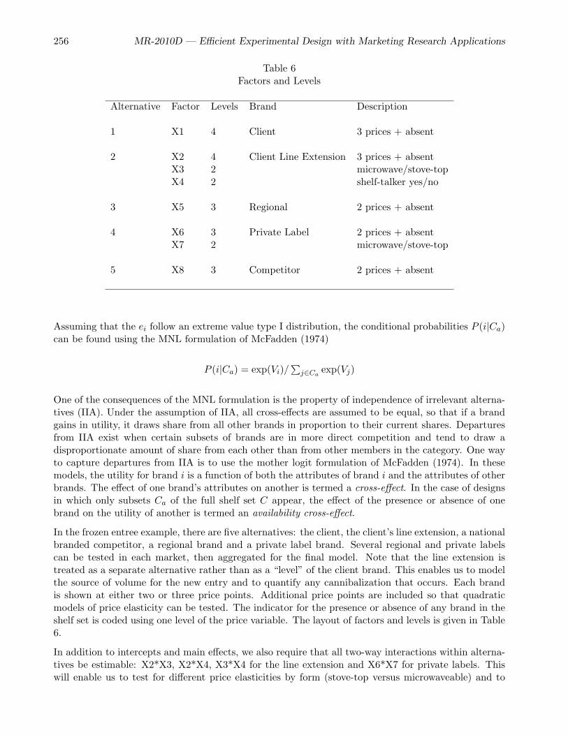
Table 6Factors and Levels

Alternative Factor Levels Brand Description

1 X1 4 Client 3 prices + absent

2 X2 4 Client Line Extension 3 prices + absentX3 2 microwave/stove-topX4 2 shelf-talker yes/no

3 X5 3 Regional 2 prices + absent

4 X6 3 Private Label 2 prices + absentX7 2 microwave/stove-top

5 X8 3 Competitor 2 prices + absent

Assuming that the ei follow an extreme value type I distribution, the conditional probabilities P (i|Ca)can be found using the MNL formulation of McFadden (1974)

P (i|Ca) = exp(Vi)/∑

j∈Caexp(Vj)

One of the consequences of the MNL formulation is the property of independence of irrelevant alterna-tives (IIA). Under the assumption of IIA, all cross-effects are assumed to be equal, so that if a brandgains in utility, it draws share from all other brands in proportion to their current shares. Departuresfrom IIA exist when certain subsets of brands are in more direct competition and tend to draw adisproportionate amount of share from each other than from other members in the category. One wayto capture departures from IIA is to use the mother logit formulation of McFadden (1974). In thesemodels, the utility for brand i is a function of both the attributes of brand i and the attributes of otherbrands. The effect of one brand’s attributes on another is termed a cross-effect. In the case of designsin which only subsets Ca of the full shelf set C appear, the effect of the presence or absence of onebrand on the utility of another is termed an availability cross-effect.

In the frozen entree example, there are five alternatives: the client, the client’s line extension, a nationalbranded competitor, a regional brand and a private label brand. Several regional and private labelscan be tested in each market, then aggregated for the final model. Note that the line extension istreated as a separate alternative rather than as a “level” of the client brand. This enables us to modelthe source of volume for the new entry and to quantify any cannibalization that occurs. Each brandis shown at either two or three price points. Additional price points are included so that quadraticmodels of price elasticity can be tested. The indicator for the presence or absence of any brand in theshelf set is coded using one level of the price variable. The layout of factors and levels is given in Table6.

In addition to intercepts and main effects, we also require that all two-way interactions within alterna-tives be estimable: X2*X3, X2*X4, X3*X4 for the line extension and X6*X7 for private labels. Thiswill enable us to test for different price elasticities by form (stove-top versus microwaveable) and to


see if the promotion works better combined with a low price or with different forms. Using a linearmodel for X1-X8, the total number of parameters including the intercept, all main effects, and two-wayinteractions with brand is 25. This assumes that price is treated as qualitative. The actual numberof parameters in the choice model is larger than this because of the inclusion of cross-effects. Usingindicator variables to code availability, the systematic component of utility for brand i can be expressedas:

Vi = ai +∑

k(bik × xik) +∑

j 6=i zj(dij +∑

l(gijl × xjl))

where

ai = intercept for brand ibik = effect of attribute k for brand i, where k = 1, ..,Ki

xik = level of attribute k for brand idij = availability cross-effect of brand j on brand i

zj = availability code =

{1 if j ∈ Ca,0 otherwise

gijl = cross-effect of attribute l for brand j on brand i, where l = 1, .., Lj

xjl = level of attribute l for brand j.

The xik and xjl might be expanded to include interaction and polynomial terms. In an availabilitycross-effects design, each brand is present in only a fraction of choice sets. The size of this fractionor subdesign is a function of the number of levels of the alternative-specific variable that is used tocode availability (usually price). For example, if price has three valid levels and a fourth “zero” levelto indicate absence, then the brand will appear in only three out of four runs. Following Lazari andAnderson (1994), the size of each subdesign determines how many model equations can be written foreach brand in the discrete choice model. If Xi is the subdesign matrix corresponding to Vi, then eachXi must be full rank to ensure that the choice set design provides estimates for all parameters.

To create the design, a full candidate set is generated consisting of 3456 runs. It is then reduced to 2776runs that contain between two and four brands so that the respondent is never required to comparemore than four brands at a time. In the algorithm model specification, we designate all variables asclassification variables and require that all main effects and two-way interactions within brands beestimable. The number of runs to use follows from a calculation of the number of parameters thatwe wish to estimate in the various submatrices Xi of X. Assuming that there is a category “None”used as a reference cell, the numbers of parameters required for various alternatives are shown in theTable 7 along with the size of submatrices (rounded down) for various numbers of runs. Parametersfor quadratic price models are given in parentheses. Note that the effect of private label being in amicrowaveable or stove-top form (stove/micro cross-effect) is an explicit parameter under the clientline extension.

The number of runs chosen was N=26. This number provides adequate degrees of freedom for thelinear price model and will also allow estimation of direct quadratic price effects. To estimate quadraticcross-effects for price would require 32 runs at the very least. Although the technique of using two-wayinteractions between nominal level variables will usually guarantee that all direct and cross-effects areestimable, it is sometimes necessary and a good practice to check the ranks of the submatrices for morecomplex models (Lazari and Anderson 1994). Creating designs for cross-effects can be difficult, evenwith the aid of a computer.


Table 7Parameters

Client PrivateEffect Client Line Extension Regional Label Competitor

intercept 1 1 1 1 1availability cross-effects 4 4 4 4 4direct price effect 1 (2) 1 (2) 1 1 1price cross-effects 4 (8) 4 (8) 4 4 4stove versus microwave - 1 - 1 -stove/micro cross-effects - 1 - - -shelf-talker - 1 - - -price*stove/microwave - 1 (2) - 1 -price*shelf-talker - 1 (2) - - -stove/micro*shelf-talker - 1 - - -

Total 10 (15) 16 (23) 10 12 10

Subdesign size

22 runs 16 16 14 14 1426 runs 19 19 17 17 1732 runs 24 24 21 21 21

It took approximately 4.5 minutes to generate a design. The final (unrandomized) design in 26 runs isin table A6.† The coded choice sets are presented in Table A7 and the level frequencies are presentedin Table A8. Note that the runs have been ordered by the presence/absence of the shelf-talker. Thisordering is done because it is unrealistic to think that once the respondent’s attention has been drawnin by the promotion, it can just be “undrawn.” The two blocks that result may be shown to two groupsof people or to the same people sequentially. It would be extremely difficult and time consuming togenerate a design for this problem without a computerized algorithm.

Conjoint Analysis with Aggregate Interactions. This example illustrates creating a design for aconjoint analysis study. The goal is to create a 36 design in 90 runs. The design consists of five blocksof 18 runs each, so each subject will only have to rate 18 products. Within each block, main-effectsmust be estimable. In the aggregate, all main-effects and two-way interactions must be estimable.(The utilities from the main-effects models will be used to cluster subjects, then in the aggregateanalysis, clusters of subjects will be pooled across blocks and the blocking factor ignored.) Our goalis to create a design that is simultaneously efficient in six ways. Each of the five blocks should bean efficient design for a first-order (main-effects) model, and the aggregate design should be efficientfor the second-order (main-effects and two-way interactions) model. The main-effects models for thefive blocks have 5(1 + 6(3 − 1)) = 65 parameters. In addition, there are (6 × 5/2)(3 − 1)(3 − 1) = 60parameters for interactions in the aggregate model. There are more parameters than runs, but not all

†This is the design that was presented in the original 1994 paper, which due to differences in the random numberseeds, is not reproduced by today’s tools.


parameters will be simultaneously estimated.

One approach to this problem is the Bayesian regression method of DuMouchell and Jones (1994).Instead of optimizing |X′X|, we optimized |X′X+P|, where P is a diagonal matrix of prior precisions.This is analogous to ridge regression, in which a diagonal matrix is added to a rank-deficient X′X tocreate a full-rank problem. We specified a model with a blocking variable, main effects for the sixfactors, block-effect interactions for the six factors, and all two-way interactions. We constructed P tocontain zeros for the blocking variable, main effects, and block-effect interactions, and 45s (the numberof runs divided by 2) for the two-way interactions. Then we used the modified Fedorov algorithm tosearch for good designs.

With an appropriate coding for X, the value of the prior precision for a parameter roughly reflects thenumber of runs worth of prior information available for that parameter. The larger the prior precisionfor a parameter, the less information about that parameter is in the final design. Specifying a nonzeroprior precision for a parameter reduces the contribution of that parameter to the overall efficiency. Forthis problem, we wanted maximal efficiency for the within-subject main-effects models, so we gave anonzero prior precision to the aggregated two-way interactions.

Our best design had a D-efficiency for the second-order model of 63.9281 (with a D-efficiency for theaggregate main-effects model of 99.4338) and D-efficiencies for the main-effects models within eachblock of 100.0000, 100.0000, 100.0000, 99.0981, and 98.0854. The design is completely balanced withinall blocks. We could have specified other values in P and gotten better efficiency for the aggregatedesign but less efficiency for the blocks. Choice of P depends in part on the primary goals of theexperiment. It may require some simulation work to determine a good choice of P.

All of the examples in this article so far have been straight-forward applications of computerized designmethodology. A set of factors, levels, and estimable effects was specified, and the computer looked foran efficient design for that specification. Simple problems, such as those discussed previously, requireonly a few minutes of computer time. This problem was much more difficult, so we let a work stationgenerate designs for about 72 hours. (We could have found less efficient but still acceptable designs inmuch less time.) We were asking the computer to find a good design out of over 9.6×10116 possibilities.This is like looking for a needle in a haystack, when the haystack is the size of the entire known universe.With such problems, we may do better if we use our intuition to give the computer “hints,” forcingcertain structure into the design. To illustrate, we tried this problem again, this time using a differentapproach.

We used the modified Fedorov algorithm to generate main-effects only 36 designs in 18 runs. Westopped when we had ten designs all with 100% efficiency. We then wrote an ad hoc program thatrandomly selected five of the ten designs, randomly permuted columns within each block, and randomlypermuted levels within each block. These operations do not affect the first-order efficiencies but doaffect the overall efficiency for the aggregate design. When an operation increased efficiency, the newdesign was kept. We iterated over the entire design 20 times. We let the program run for about 16hours, which generated 98 designs, and we found our best design in three hours. Our best design hada D-efficiency for the second-order model of 68.0565 (versus 63.9281 previously), and all first-orderefficiencies of 100.

Many other variations on this approach could be tried. For example, columns and blocks could bechosen at random, instead of systematically. We performed excursions of up to eight permutationsbefore we reverted to the previous design. This number could be varied. It seemed that permutingthe levels helped more than permuting the columns, though this was not thoroughly investigated.Whatever is done, it is important to consider efficiency. For example, just randomly permuting levelscan create very inefficient designs.


For this particular problem, the ad hoc algorithm generated better designs than the Bayesian method,and it required less computer time. In fact, 91 out of the 98 ad hoc designs were better than the bestBayesian design. However, the ad hoc method required much more programmer time. It is possible tomanually create a design for this situation, but it would be extremely difficult and time consuming tofind an efficient design without a computerized algorithm for all but the most sophisticated of humandesigners. The best designs were found when used both our human design skills and a computerizedsearch. We have frequently found this to be the case.

Conclusions

Computer-generated experimental designs can provide both better and more general designs for discrete-choice and preference-based conjoint studies. Classical designs, obtained from books or computerizedtables, can be good options when they exist, but they are not the only option. The time-consuming andpotentially error-prone process of finding and manually modifying an existing design can be avoided.When the design is nonstandard and there are restrictions, a computer can generate a design, and it canbe done quickly. In most situations, a good design can be generated in a few minutes or hours, thoughfor certain difficult problems more time may be necessary. Furthermore, when the circumstances ofthe project change, a new design can again be generated quickly.

We do not argue that computerized searches for D-efficient designs are uniformly superior to manuallygenerated designs. The human designer, using intuition, experience, and heuristics, can recognizestructure that an optimization algorithm cannot. On the other hand, the computerized search usuallydoes a good job, it is easy to use, and it can create a design faster than manual methods, especiallyfor the nonexpert. Computerized search methods and the use of efficiency criteria can benefit expertdesigners as well. For example, the expert can manually generate a design and then use the computerto evaluate and perhaps improve its efficiency.

In nonstandard situations, simultaneous balance and orthogonality may be unobtainable. Often, thebest that can be hoped for is optimal efficiency. Computerized algorithms help by searching for the mostefficient designs from a potentially very large set of possible designs. Computerized search algorithmsfor D-efficient designs do not supplant traditional design-creation skills. Rather, they provide helpfultools for finding good, efficient experimental designs.


Table A1Chakravarti’s L18, Factor Levels

X1 X2 X3 X4 X5

-1 -1 -1 -1 -1-1 -1 0 0 1-1 -1 1 1 0-1 1 -1 1 0-1 1 0 -1 -1-1 1 1 0 11 -1 -1 0 01 -1 -1 1 11 -1 0 -1 01 -1 0 1 -11 -1 1 -1 11 -1 1 0 -11 1 -1 -1 11 1 -1 0 -11 1 0 0 01 1 0 1 11 1 1 -1 01 1 1 1 -1

Table A2Chakravarti’s L18, Orthogonal Coding

X1 X2 X3 - X4 - X5 -

-1 -1 -1.225 -0.707 -1.225 -0.707 -1.225 -0.707-1 -1 0.000 1.414 0.000 1.414 1.225 -0.707-1 -1 1.225 -0.707 1.225 -0.707 0.000 1.414-1 1 -1.225 -0.707 1.225 -0.707 0.000 1.414-1 1 0.000 1.414 -1.225 -0.707 -1.225 -0.707-1 1 1.225 -0.707 0.000 1.414 1.225 -0.7071 -1 -1.225 -0.707 0.000 1.414 0.000 1.4141 -1 -1.225 -0.707 1.225 -0.707 1.225 -0.7071 -1 0.000 1.414 -1.225 -0.707 0.000 1.4141 -1 0.000 1.414 1.225 -0.707 -1.225 -0.7071 -1 1.225 -0.707 -1.225 -0.707 1.225 -0.7071 -1 1.225 -0.707 0.000 1.414 -1.225 -0.7071 1 -1.225 -0.707 -1.225 -0.707 1.225 -0.7071 1 -1.225 -0.707 0.000 1.414 -1.225 -0.7071 1 0.000 1.414 0.000 1.414 0.000 1.4141 1 0.000 1.414 1.225 -0.707 1.225 -0.7071 1 1.225 -0.707 -1.225 -0.707 0.000 1.4141 1 1.225 -0.707 1.225 -0.707 -1.225 -0.707


Table A3Green & Wind

Orthogonal DesignExample

X1 X2 X3 X4 X5

-1 -1 -1 -1 -1-1 -1 -1 1 0-1 -1 0 -1 -1-1 -1 0 0 1-1 -1 0 1 -1-1 -1 1 -1 0-1 -1 1 0 1-1 -1 1 1 0-1 1 -1 1 1-1 1 -1 -1 1-1 1 0 0 0-1 1 1 0 -11 -1 -1 0 -11 -1 -1 0 01 -1 0 1 11 -1 1 -1 11 1 1 1 -11 1 0 -1 0

Table A4Information-Efficient

Design,Factor Levels

X1 X2 X3 X4 X5

-1 -1 -1 0 -1-1 -1 0 -1 0-1 -1 0 1 -1-1 -1 1 0 1-1 -1 1 1 1-1 1 -1 -1 0-1 1 -1 0 -1-1 1 0 -1 1-1 1 1 1 01 -1 -1 -1 11 -1 -1 1 01 -1 0 0 01 -1 1 -1 -11 1 -1 1 11 1 0 0 11 1 0 1 -11 1 1 -1 -11 1 1 0 0

Table A5Information-EfficientDesign, Unrealistic

Combinations Excluded

X1 X2 X3 X4 X5

-1 -1 -1 1 0-1 -1 -1 -1 1-1 -1 -1 0 -1-1 -1 0 -1 1-1 -1 0 0 0-1 1 1 1 0-1 1 1 -1 -1-1 1 1 0 1-1 1 0 1 -11 -1 1 1 -11 -1 1 -1 01 -1 1 0 11 -1 0 1 -11 1 -1 1 01 1 -1 -1 -11 1 -1 0 11 1 0 -1 11 1 0 0 0

Table A6Consumer Food Product (Raw) Design

X1 X2 X3 X4 X5 X6 X7 X8

1 1 2 1 1 2 1 31 2 2 1 2 3 1 21 4 1 1 1 3 1 32 2 1 1 3 2 1 12 3 2 1 2 2 2 32 4 2 1 3 3 2 23 1 1 1 3 2 2 23 3 2 1 3 1 2 13 4 2 1 2 1 1 14 1 1 1 2 3 2 14 1 2 1 3 3 1 14 2 2 1 1 2 2 34 3 1 1 1 1 1 2

1 3 1 2 3 2 2 11 3 2 2 3 1 1 31 4 2 2 1 1 2 12 1 1 2 1 3 1 12 2 2 2 3 2 1 12 3 1 2 2 1 2 32 4 1 2 3 1 1 23 1 2 2 2 3 2 23 2 1 2 1 3 2 33 4 2 2 2 3 1 34 1 1 2 3 2 1 34 2 1 2 2 1 2 24 3 2 2 1 2 1 2


Table A7Consumer Food Product Choice Set

Block 1: Shelf-Talker Absent For Client Line Extension

Choice Client Client Line Regional Private NationalSet Brand Extension Brand Label Competitor

1 $1.29 $1.39/stove $1.99 $2.29/micro N/A2 $1.29 $1.89/stove $2.49 N/A $2.393 $1.29 N/A $1.99 N/A N/A4 $1.69 $1.89/micro N/A $2.29/micro $1.995 $1.69 $2.39/stove $2.49 $2.29/stove N/A6 $1.69 N/A N/A N/A $2.397 $2.09 $1.39/micro N/A $2.29/stove $2.398 $2.09 $2.39/stove N/A $1.49/stove $1.999 $2.09 N/A $2.49 $1.49/micro $1.99

10 N/A $1.39/micro $2.49 N/A $1.9911 N/A $1.39/stove N/A N/A $1.9912 N/A $1.89/stove $1.99 $2.29/stove N/A13 N/A $2.39/micro $1.99 $1.49/micro $2.39

Block 2: Shelf-Talker Present For Client Line Extension

Choice Client Client Line Regional Private NationalSet Brand Extension Brand Label Competitor

14 $1.29 $2.39/micro N/A $2.29/stove $1.9915 $1.29 $2.39/stove N/A $1.49/micro N/A16 $1.29 N/A $1.99 $1.49/stove $1.9917 $1.69 $1.39/micro $1.99 N/A $1.9918 $1.69 $1.89/stove N/A $2.29/micro $1.9919 $1.69 $2.39/micro $2.49 $1.49/stove N/A20 $1.69 N/A N/A $1.49/micro $2.3921 $2.09 $1.39/stove $2.49 N/A $2.3922 $2.09 $1.89/micro $1.99 N/A N/A23 $2.09 N/A $2.49 N/A N/A24 N/A $1.39/micro N/A $2.29/micro N/A25 N/A $1.89/micro $2.49 $1.49/stove $2.3926 N/A $2.39/stove $1.99 $2.29/micro $2.39

Table A8Consumer Food Product Design Level Frequencies

Level X1 X2 X3 X4 X5 X6 X7 X8

1 6 7 12 13 8 8 14 92 7 6 14 13 8 9 12 83 6 7 10 9 94 7 6


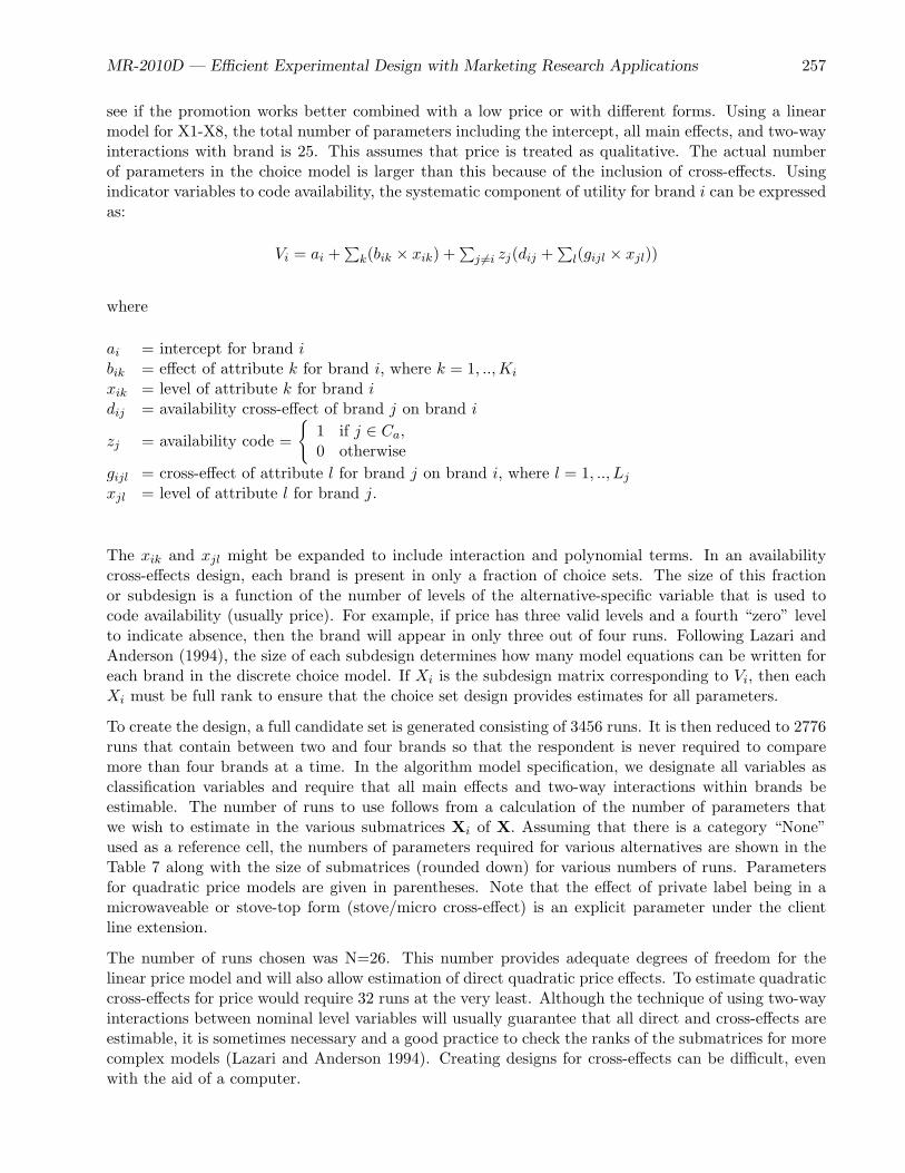
Table A9Consumer Food Product Design Creation Code

*-----------------------------------------------------*| Construct the Design. |*-----------------------------------------------------;

%macro bad;bad = (x1 < 4) + (x2 < 4) + (x5 < 3) + (x6 < 3) + (x8 < 3);bad = abs(bad - 3) * ((bad < 2) | (bad > 4));%mend;

%mktex(4 4 2 2 3 3 2 3, n=26, interact=x2*x3 x2*x4 x3*x4 x6*x7,restrictions=bad, outr=sasuser.choicdes)

*-----------------------------------------------------*| Print the Design. |*-----------------------------------------------------;

proc format;value yn 1 = ’No’ 2 = ’Talker’;value micro 1 = ’Micro’ 2 = ’Stove’;run;

data key;missing N;input x1-x8;format x1 x2 x5 x6 x8 dollar5.2

x4 yn. x3 x7 micro.;label x1 = ’Client Brand’

x2 = ’Client Line Extension’x3 = ’Client Micro/Stove’x4 = ’Shelf Talker’x5 = ’Regional Brand’x6 = ’Private Label’x7 = ’Private Micro/Stove’x8 = ’National Competitor’;

datalines;1.29 1.39 1 1 1.99 1.49 1 1.991.69 1.89 2 2 2.49 2.29 2 2.392.09 2.39 . . N N . NN N . . . . . .;

%mktlab(data=sasuser.choicdes, key=key)

proc sort out=sasuser.finchdes; by x4; run;

proc print label; id x4; by x4; run;

eﬃcient experimental design with marketing research...

Documents