gaussian processes for sample efficient reinforcement
TRANSCRIPT

To appear in The European Conference on Machine Learning (ECML 2010),Barcelona, Spain, September 2010.
Gaussian processes for sample efficient
reinforcement learning with RMAX-like
exploration
Tobias Jung1 and Peter Stone1
tjung,[email protected]
Department of Computer ScienceUniversity of Texas at Austin
Abstract. We present an implementation of model-based online rein-forcement learning (RL) for continuous domains with deterministic tran-sitions that is specifically designed to achieve low sample complexity. Toachieve low sample complexity, since the environment is unknown, anagent must intelligently balance exploration and exploitation, and mustbe able to rapidly generalize from observations. While in the past a num-ber of related sample efficient RL algorithms have been proposed, to al-low theoretical analysis, mainly model-learners with weak generalizationcapabilities were considered. Here, we separate function approximationin the model learner (which does require samples) from the interpolationin the planner (which does not require samples). For model-learning weapply Gaussian processes regression (GP) which is able to automaticallyadjust itself to the complexity of the problem (via Bayesian hyperpa-rameter selection) and, in practice, often able to learn a highly accu-rate model from very little data. In addition, a GP provides a naturalway to determine the uncertainty of its predictions, which allows us toimplement the “optimism in the face of uncertainty” principle used toefficiently control exploration. Our method is evaluated on four commonbenchmark domains.
1 Introduction
In reinforcement learning (RL), an agent interacts with an environment andattempts to choose its actions such that an externally defined performance mea-sure, the accumulated per-step reward, is maximized over time. One definingcharacteristic of RL is that the environment is unknown and that the agent hasto learn how to act directly from experience. In practical applications, e.g., inrobotics, obtaining this experience means having a physical system interact withthe physical environment in real time. Therefore, RL methods that are able tolearn quickly and minimize the amount of time the robot needs to interact withthe environment until good or optimal behavior is learned, are highly desirable.
In this paper we are interested in online RL for tasks with continuous statespaces and smooth transition dynamics that are typical for robotic control do-mains. Our primary goal is to have an algorithm which keeps sample complexityas low as possible.
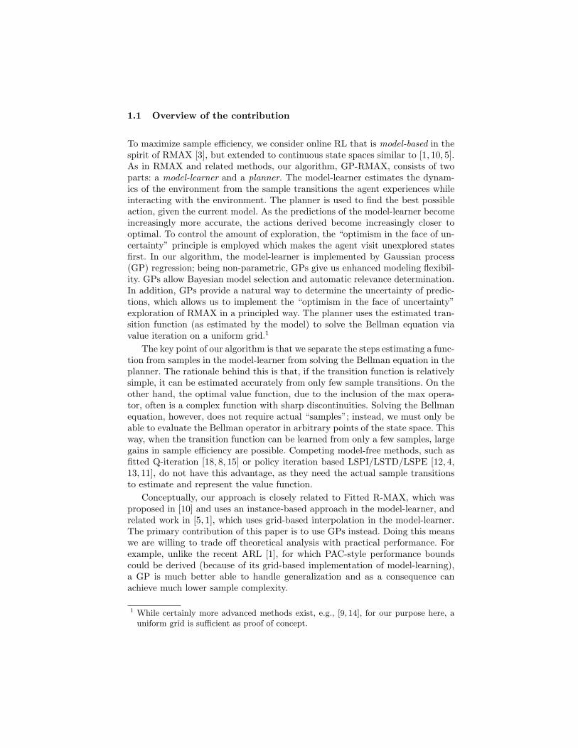
1.1 Overview of the contribution
To maximize sample efficiency, we consider online RL that is model-based in thespirit of RMAX [3], but extended to continuous state spaces similar to [1, 10, 5].As in RMAX and related methods, our algorithm, GP-RMAX, consists of twoparts: a model-learner and a planner. The model-learner estimates the dynam-ics of the environment from the sample transitions the agent experiences whileinteracting with the environment. The planner is used to find the best possibleaction, given the current model. As the predictions of the model-learner becomeincreasingly more accurate, the actions derived become increasingly closer tooptimal. To control the amount of exploration, the “optimism in the face of un-certainty” principle is employed which makes the agent visit unexplored statesfirst. In our algorithm, the model-learner is implemented by Gaussian process(GP) regression; being non-parametric, GPs give us enhanced modeling flexibil-ity. GPs allow Bayesian model selection and automatic relevance determination.In addition, GPs provide a natural way to determine the uncertainty of predic-tions, which allows us to implement the “optimism in the face of uncertainty”exploration of RMAX in a principled way. The planner uses the estimated tran-sition function (as estimated by the model) to solve the Bellman equation viavalue iteration on a uniform grid.1
The key point of our algorithm is that we separate the steps estimating a func-tion from samples in the model-learner from solving the Bellman equation in theplanner. The rationale behind this is that, if the transition function is relativelysimple, it can be estimated accurately from only few sample transitions. On theother hand, the optimal value function, due to the inclusion of the max opera-tor, often is a complex function with sharp discontinuities. Solving the Bellmanequation, however, does not require actual “samples”; instead, we must only beable to evaluate the Bellman operator in arbitrary points of the state space. Thisway, when the transition function can be learned from only a few samples, largegains in sample efficiency are possible. Competing model-free methods, such asfitted Q-iteration [18, 8, 15] or policy iteration based LSPI/LSTD/LSPE [12, 4,13, 11], do not have this advantage, as they need the actual sample transitionsto estimate and represent the value function.
Conceptually, our approach is closely related to Fitted R-MAX, which wasproposed in [10] and uses an instance-based approach in the model-learner, andrelated work in [5, 1], which uses grid-based interpolation in the model-learner.The primary contribution of this paper is to use GPs instead. Doing this meanswe are willing to trade off theoretical analysis with practical performance. Forexample, unlike the recent ARL [1], for which PAC-style performance boundscould be derived (because of its grid-based implementation of model-learning),a GP is much better able to handle generalization and as a consequence canachieve much lower sample complexity.
1 While certainly more advanced methods exist, e.g., [9, 14], for our purpose here, auniform grid is sufficient as proof of concept.

1.2 Assumptions and limitations
Our approach makes the following assumptions (most of which are also made inrelated work, even if it is not always explicitly stated):
– Low dimensionality of the state space. With a uniform grid, the numberof grid points for solving the Bellman equation scales exponentially withthe dimensionality. While more advanced methods, such as sparse grids oradaptive grids, may allow us to somewhat reduce this exponential increase, atthe end they do not break the curse of dimensionality. Alternatively, one canuse nonlinear function approximation; however, despite some encouragingresults, it is unclear as to whether this approach would really do any betterin general applications. Today, breaking the curse of dimensionality is stillan open research problem.
– Discrete actions. While continuous actions may be discretized, in practice,for higher dimensional action spaces this becomes infeasible.
– Smooth transition function. Performing an action from states that are “close”must lead to successor states that are “close”. (Otherwise both the gener-alization in the model learner and the interpolation in the value functionapproximation would not work).
– Deterministic transitions. This is not a fundamental requirement of our ap-proach, since GPs can also learn noisy functions (either due to observationnoise or random disturbances with small magnitude), and the Bellman op-erator can be evaluated in the resulting predictive distribution. Rather it isone taken for convenience.
– Known reward function. Assuming that the reward function is known andonly the transition function needs to be learned is what is different from mostcomparable work. While it is not a fundamental requirement of our approach(since we could learn the reward function as well), it is an assumption thatwe think is well justified: for one, reward is the performance criterion andspecifies the goal. For the type of control problems we consider here, rewardis always externally defined and never something that is “generated” fromwithin the environment. Two, reward sometimes is a discontinuous function,e.g., +1 at the goal state and 0 elsewhere. Which makes it not very amenablefor function approximation.
2 Background: Planning when the model is exact
Consider the reinforcement learning problem for MDPs with continuous statespace, finite action space, discounted reward criterion and deterministic dynam-ics [19]. In this section we assume that dynamics and rewards are available to thelearning agent. Let state space X be a hyperrectangle in Rd (this assumption isjustified if, for example, the system is a motor control task), A be the finite ac-tion space (assuming continuous controls are discretized), xt+1 = f(xt, at) be thetransition function (assuming that continuous time problems are discretized intime), and r(x, a) be the reward function. For the following theoretical argument

ξ00
ξ10 ξ11
ξ01
Q(z, a′) =?
z := f(ξi, a)
ξi
transition f
dx
dy
hx
hy
z = (x, y)
x0
x1
(ξ00, qa′
00)
(ξ10, qa′
10) (ξ11, qa′
11)
(ξ01, qa′
01)
Fig. 1. Bilinear interpolation to determine Q(f(ξi, a), a′) in R2.
we require that both transition and reward function are Lipschitz continuous inthe actions; i.e., there exist constants Lf , Lr such that ‖f(x, a) − f(x′, a)‖ ≤Lf ‖x − x′‖, and |r(x, a) − r(x′, a)| ≤ Lr ‖x − x′‖, ∀x, x′ ∈ X , a ∈ A. In addi-tion, we assume that the reward is bounded, |r(x, a)| ≤ RMAX, ∀x, a. Note thatin practice, while the first condition, continuity in the transition function, is usu-ally fulfilled for domains derived from physical systems, the second condition,continuity in the rewards, is often violated (e.g. in the mountain car domain,reward is 0 in the goal and −1 everywhere else). Despite that we find that inmany of these cases the outlined procedure may still work well enough.
For any state x, we are interested in determining a sequence of actionsa0, a1, a2, . . . such that the accumulated reward is maximized,
V ∗(x) := maxa0,a1,...
∞∑
t=0
γtr(xt, at) | x0 = x, xt+1 = f(xt, at)
,
where 0 < γ < 1. Using the Q-notation, where Q∗(x, a) := r(x, a)+γV ∗(f(x, a)),the optimal decision policy π∗ is found by first solving the Bellman equation inthe unknown function Q,
Q(x, a) = r(x, a) + γ maxa′
Q(f(x, a), a′) ∀x ∈ X , a ∈ A (1)
to yield Q∗, and then choosing the action with the highest Q-value,
π∗(x) = argmaxa′
Q∗(x, a′).
The Bellman operator T related to (1) is defined by
(
TQ)
(x, a) := r(x, a) + γ maxa′
Q(f(x, a), a′). (2)
It is well known that T is a contraction and Q∗ the unique bounded solution tothe fixed point problem Q(x, a) =
(
TQ)
(x, a), ∀x, a.

In order to solve the infinite dimensional problem in (1) numerically, wehave to reduce it to a finite dimensional problem. This is done by introducinga discretization Γ of X into a finite number of elements, applying the Bellmanoperator to only the nodes and interpolating in between.
In the following we will consider a uniform grid Γh with N vertices ξi andd-dimensional tensor B-spline interpolation of order 1. The solution of (1) isthen obtained in the space of piecewise affine functions.
For a fixed action a′, the value QΓh(z, a′) of any state z with respect togrid Γh can be written as a convex combination of the vertices ξj of the gridcell enclosing z with coefficients wij (see Figure 1a). For example, consider the2-dimensional case (bilinear interpolation) in Figure 1b. Let z = (x, y) ∈ R2.To determine QΓh(z, a′), we find the four vertices ξ00, ξ01, ξ10, ξ11 ∈ R2 of theenclosing cell with known function values qa′
00 := QΓh(ξ00, a′), . . . etc. We then
perform two linear interpolations along the x-coordinate (order invariant) in theauxilary points x0, x1 to obtain
QΓh(x0, a′) = (1 − λ0)q
a′
00 + λ0qa′
01
QΓh(x1, a′) = (1 − λ0)q
a′
10 + λ0qa′
11
where λ0 := dx/hx (see Figure 1b for a definition of dx, hx, x0, x1). We thenperform another linear interpolation in x0, x1 along the y-coordinate to obtain
QΓh(z, a′) = (1− λ1)(1− λ0)qa′
00 + (1− λ1)λ0qa′
01 + λ1(1− λ0)qa′
10 + λ1λ0qa′
11 (3)
where λ1 := dy/hy. Weights wij now correspond to the coefficients in (3). Ananalogous procedure applies to higher dimensions.
Let Qa′
be the N×1 vector with entries [Qa′
]i = QΓh(ξi, a′). Let za
1 , . . . , zaN ∈
Rd denote the successor state we obtain when we apply the transition function
f to vertices ξi using action a, i.e., zai := f(ξi, a). Let [wa
i ]j = waij denote the
1 × N vector of coefficients for zai from (3). The Q-value of za
i for any action a′
with respect to grid Γh can thus be written as QΓh(zai , a′) =
∑N
j=1[wai ]j [Q
a′
]j .Let W a with rows [wa
i ] be the N × N matrix of all coefficients. (Note that thismatrix is sparse: each row contains only 2d nonzero entries).
Let Ra be the N × 1 vector of associated rewards, [Ra]i := r(ξi, a). Now wecan use (2) to obtain a fixed point equation in the vertices of the grid Γh,
QΓh(ξi, a) =(
TΓhQΓh)
(ξi, a) i = 1, . . . , N, a = 1, . . . , |A|, (4)
where(
TΓhQΓh)
(ξi, a) := r(ξi, a) + γ maxa′
QΓh(f(ξi, a), a′).
Slightly abusing the notation, we can write this more compactly in terms ofmatrices and vectors,
TΓhQΓh := Ra + γ maxa′
W aQa′
∀a. (5)
The Q-function is now represented by |A| N -dimensional vectors Qa′
, each con-taining the values for the vertices ξi. The discretized Bellman operator TΓh is

xt+1 = f(xt, at)
xt
xt at
(xt, at, xt+1)
f(x, a), c(x, a)
Fig. 2. High-level overview of the GP-RMAX framework
a contraction in Rd × A and therefore has a unique fixed point Q∗ ∈ Rd × A.Let function Q∗,Γh : (Rd × A) → R be the Q-function obtained by linear in-terpolation of vector Q∗ along states. The function Q∗,Γh can now be used todetermine (approximately) optimal control actions: for any state x ∈ X , wesimply determine
π∗,Γh(x) = argmaxa′
Q∗,Γh(x, a′).
In order to estimate how well function Q∗,Γh approximates the true Q∗, a poste-
riori estimates can be defined that are based on local errors, i.e. the maximumof residual in each grid cell. The local error in a grid cell in turn depends on thegranularity of the grid, h, and the modulus of continuity Lf , Lg (e.g., see [9, 14]for details).
3 Our algorithm: GP-RMAX
In the last section we have seen how, for a continuous state space, optimalbehavior of an agent can be obtained in a numerically robust way, given thatthe transition function xt+1 = f(xt, at) is known.2
For model-based RL we are now interested in solving the same problem forthe case that the transition function is not known. Instead, the agent has tointeract with the environment, and only use the samples it observes to computeoptimal behavior. Our goal in this paper is to develop a learning framework
2 Remember our working assumption: reward as a performance criterion is externallygiven and does not need to be estimated by the agent. Also note that discretization(even with more advanced methods like adaptive or sparse grids) is likely to befeasible only in state spaces with low to medium dimensionality. Breaking the curseof dimensionality is an open research problem.
where this number is kept as small as possible. This will be done by using thesamples to learn an estimate f(x, a) of f(x, a) and then use this estimate f inplace of f in the numerical procedure outlined in the previous section.
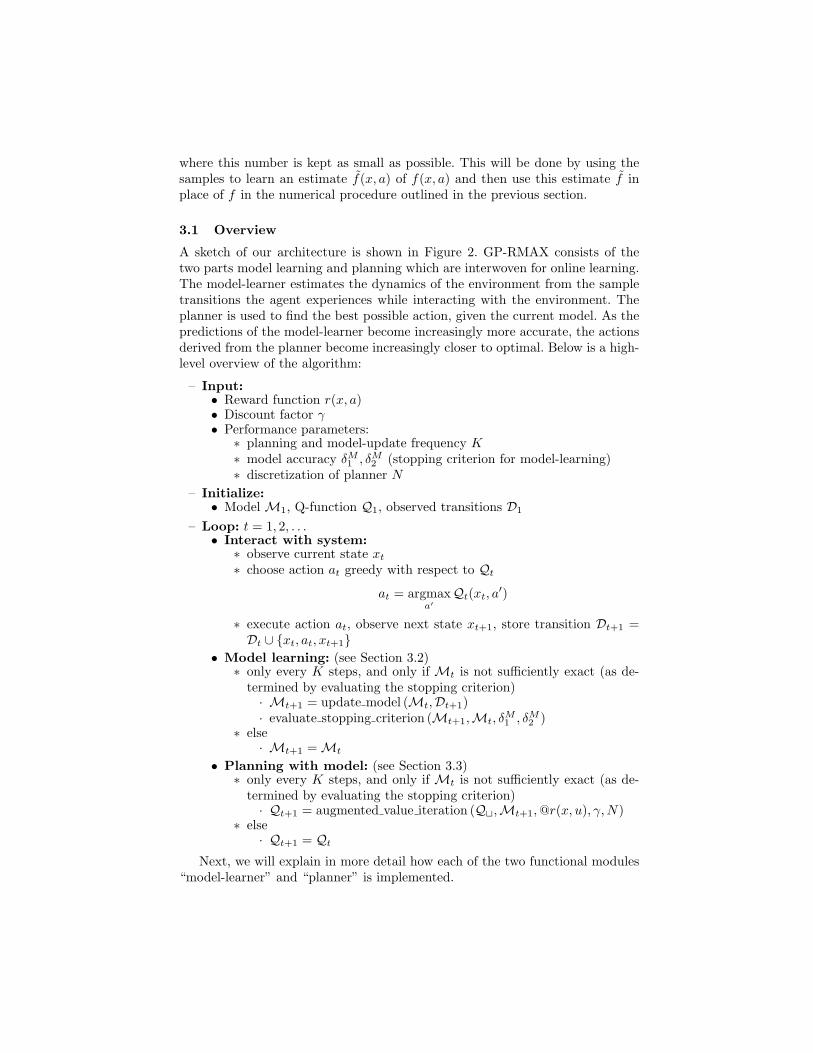
3.1 Overview
A sketch of our architecture is shown in Figure 2. GP-RMAX consists of thetwo parts model learning and planning which are interwoven for online learning.The model-learner estimates the dynamics of the environment from the sampletransitions the agent experiences while interacting with the environment. Theplanner is used to find the best possible action, given the current model. As thepredictions of the model-learner become increasingly more accurate, the actionsderived from the planner become increasingly closer to optimal. Below is a high-level overview of the algorithm:
– Input:• Reward function r(x, a)• Discount factor γ• Performance parameters:
∗ planning and model-update frequency K∗ model accuracy δM
1 , δM2 (stopping criterion for model-learning)
∗ discretization of planner N
– Initialize:• Model M1, Q-function Q1, observed transitions D1
– Loop: t = 1, 2, . . .• Interact with system:
∗ observe current state xt
∗ choose action at greedy with respect to Qt
at = argmaxa′
Qt(xt, a′)
∗ execute action at, observe next state xt+1, store transition Dt+1 =Dt ∪ xt, at, xt+1
• Model learning: (see Section 3.2)∗ only every K steps, and only if Mt is not sufficiently exact (as de-
termined by evaluating the stopping criterion)· Mt+1 = update model (Mt,Dt+1)· evaluate stopping criterion (Mt+1,Mt, δ
M1 , δM
2 )∗ else
· Mt+1 = Mt
• Planning with model: (see Section 3.3)∗ only every K steps, and only if Mt is not sufficiently exact (as de-
termined by evaluating the stopping criterion)· Qt+1 = augmented value iteration (Q⊔,Mt+1,@r(x, u), γ,N)
∗ else· Qt+1 = Qt
Next, we will explain in more detail how each of the two functional modules“model-learner” and “planner” is implemented.
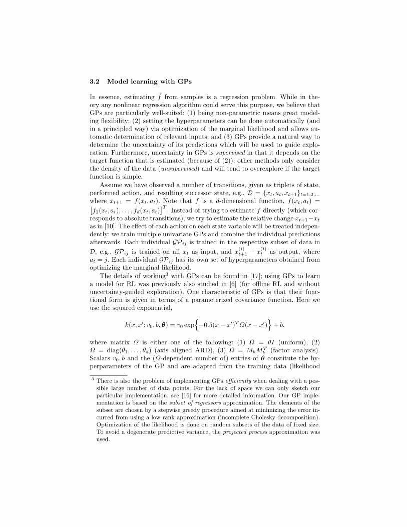
3.2 Model learning with GPs
In essence, estimating f from samples is a regression problem. While in the-ory any nonlinear regression algorithm could serve this purpose, we believe thatGPs are particularly well-suited: (1) being non-parametric means great model-ing flexibility; (2) setting the hyperparameters can be done automatically (andin a principled way) via optimization of the marginal likelihood and allows au-tomatic determination of relevant inputs; and (3) GPs provide a natural way todetermine the uncertainty of its predictions which will be used to guide explo-ration. Furthermore, uncertainty in GPs is supervised in that it depends on thetarget function that is estimated (because of (2)); other methods only considerthe density of the data (unsupervised) and will tend to overexplore if the targetfunction is simple.
Assume we have observed a number of transitions, given as triplets of state,performed action, and resulting successor state, e.g., D = xt, at, xt+1t=1,2,...
where xt+1 = f(xt, at). Note that f is a d-dimensional function, f(xt, at) =[
f1(xt, at), . . . , fd(xt, at)]T
. Instead of trying to estimate f directly (which cor-responds to absolute transitions), we try to estimate the relative change xt+1−xt
as in [10]. The effect of each action on each state variable will be treated indepen-dently: we train multiple univariate GPs and combine the individual predictionsafterwards. Each individual GPij is trained in the respective subset of data in
D, e.g., GPij is trained on all xt as input, and x(i)t+1 − x
(i)t as output, where
at = j. Each individual GPij has its own set of hyperparameters obtained fromoptimizing the marginal likelihood.
The details of working3 with GPs can be found in [17]; using GPs to learna model for RL was previously also studied in [6] (for offline RL and withoutuncertainty-guided exploration). One characteristic of GPs is that their func-tional form is given in terms of a parameterized covariance function. Here weuse the squared exponential,
k(x, x′; v0, b,θ) = v0 exp
−0.5(x − x′)T Ω(x − x′)
+ b,
where matrix Ω is either one of the following: (1) Ω = θI (uniform), (2)Ω = diag(θ1, . . . , θd) (axis aligned ARD), (3) Ω = MkMT
k (factor analysis).Scalars v0, b and the (Ω-dependent number of) entries of θ constitute the hy-perparameters of the GP and are adapted from the training data (likelihood
3 There is also the problem of implementing GPs efficiently when dealing with a pos-sible large number of data points. For the lack of space we can only sketch ourparticular implementation, see [16] for more detailed information. Our GP imple-mentation is based on the subset of regressors approximation. The elements of thesubset are chosen by a stepwise greedy procedure aimed at minimizing the error in-curred from using a low rank approximation (incomplete Cholesky decomposition).Optimization of the likelihood is done on random subsets of the data of fixed size.To avoid a degenerate predictive variance, the projected process approximation wasused.

optimization). Note that variant (2) and (3) implement automatic relevance de-
termination: relevant inputs or linear projections of inputs are automaticallyidentified, whereby model complexity is reduced and generalization sped up.
Once trained, for any testpoint x, GPij provides a distribution over targetvalues, N (µij(x), σ2
ij(x)), with mean µij(x) and variance σ2ij(x) (exact formulas
for µ and σ can be found in [17]). Each individual mean µij predicts the changein the i-th coordinate of the state under the j-th action. Each individual varianceσ2
ij can be interpreted as the associated uncertainty; it will be close to 0 if GPij
is certain, and close to k(x, x) if it is uncertain (the value of k(x, x) depends onthe hyperparameters of GPij). Stacking the individual predictions together, ourmodel-learner produces in summary
f(x, a) :=
x(1)
...x(d)
+
µ1a(x)...
µda(x)
, c(x, a) := max
i=1,...,d
(
normalizeia(σ2ia)
)
, (6)
where f(x, a) is the predicted successor state and c(x, a) the associated un-certainty (taken as maximum over the normalized per-coordinate uncertainties,where normalization ensures that the values lie between 0 and 1).
3.3 Planning with a model
At any time t, the planner receives as input model Mt. For any state x andaction a, model Mt can be evaluated to “produce” the transition f(x, a) alongwith normalized scalar uncertainty c(x, a) ∈ [0, 1], where 0 means maximallycertain and 1 maximally uncertain (see Section 3.2)
Let Γh be the discretization of the state space X with nodes ξi, i = 1, . . . , N .We now solve the planning stage by plugging f into the procedure described inSection 2. First, we compute za
i = f(ξi, a), c(ξi, a) from (6) and the associatedinterpolation coefficients wa
ij from (3) for each node ξi and action a.Let Ca denote the N × 1 vector corresponding to the uncertainties, [Ca]i =
c(ξi, a); and Ra be the N×1 vector corresponding to the rewards, [Ra]i = r(ξi, a).To solve the discretized Bellman equation in Eq. (4), we perform basic Jacobiiteration:
– Initialize [Qa0 ]i, i = 1, . . . , N , a = 1, . . . , |A|
– Repeat for k = 0, 1, 2, . . .
[Qak+1]i = [Ra]i + γ max
a′
N∑
j=1
waij [Q
a′
k ]j
∀i, a (7)
until |Qak+1−Qa
k|∞ < tol, ∀a, or a maximum number of iterations is reached.
To reduce the number of iterations necessary, we adapt Grune’s increasing
coordinate algorithm [9] to the case of Q-functions: instead of Eq. (7), we perform

updates of the form
[Qak+1]i = [1 − γwa
ii]−1
[Ra]i + γ maxa′
N∑
j=1,j 6=i
waij [Q
a′
k ]j
. (7’)
In [9] it was proved that Eq. (7’) converges to the same fixed point as Eq. (7), andit was empirically demonstrated that convergence can occur in significantly feweriterations. The exact reduction is problem-dependent, savings will be greater forsmall γ and large cells where self-transitions occur (i.e., ξi is among the verticesof the cell enclosing za
i ).To implement the “optimism in the face of uncertainty” principle, that is, to
make the agent explore regions of the state space where the model predictionsare uncertain, we employ the heuristic modification of the Bellman operatorwhich was suggested in [15] and shown to perform well. Instead of Eq. (7’), theupdate rule becomes
[Qak+1]i = (1 − [Ca]i)[1 − γwa
ii]−1
[Ra]i + γ maxa′
N∑
j=1,j 6=i
waij [Q
a′
k ]j
+
+ [Ca]iVMAX (7”)
where VMAX := RMAX/(1 − γ). Eq. (7”) can be seen as a generalization ofthe binary uncertainty in the original RMAX paper to continuous uncertainty;whereas in RMAX a state was either “known” (sufficiently explored), in whichcase the unmodified update was used, or “unknown” (not sufficiently explored),in which case the value VMAX was assigned, here the shift from exploration toexploitation is more gradual.
Finally we can take advantage of the fact that the planning function will becalled many times during the process of learning. Since the discretization Γh iskept fixed, we can reuse the final Q-values obtained in one call to plan as initialvalues for the next call to plan. Since updates to the model often affect onlystates in some local neighborhood (in particular in later stages), the number ofnecessary iterations in each call to planning will be further reduced.
A summary of our model-based planning function is shown below.
– Input:• Model Mt, initial [Qa
0 ]i, i = 1, . . . , N , a = 1, . . . , |A|
– Static inputs:• Grid Γh with nodes ξ1, . . . , ξN , discount factor γ, reward function r(x, a)
evaluated in nodes giving [Ra]i
– Initialize:• Compute za
i = f(ξi, a) and [Ca]i from Mt (see Eq. (6))• Compute weights wa
ij for each zai (see Eq. (3))
– Loop:• Repeat update Eq. (7”) until |Qa
k+1 − Qak|∞ < tol, ∀a, or the maximum
number of iterations is reached.

4 Experiments
We now examine the online learning performance of GP-RMAX in various well-known RL benchmark domains.
4.1 Description of domains
In particular, we choose the following domains (where a large number of com-parative results is available in the literature):
Mountain car: In mountain car, the goal is to drive an underpowered car fromthe bottom of a valley to the top of one hill. The car is not powerful enough toclimb the hill directly, instead it has to build up the necessary momentum byreversing throttle and going up the hill on the opposite side first. The problemis 2-dimensional, state variable x1 ∈ [−1.2, 0.5] describes the position of the car,x2 ∈ [−0.07, 0.07] its velocity. Possible actions are a ∈ −1, 0,+1. Learning isepisodic: every step gives a reward of −1 until the top of the hill at x1 ≥ 0.5is reached. Our experimental setup (dynamics and domain specific constants) isthe same as in [19], with the following exceptions: maximal episode length is 500steps, discount factor γ = 0.99 and every episode starts with the agent being atthe bottom of the valley with zero velocity, xstart = (−π/6, 0).
Inverted pendulum: The next task is to swing up and stabilize a single-linkinverted pendulum. As in mountain car, the motor does not provide enoughtorque to push the pendulum up in a single rotation. Instead, the pendulumneeds to be swung back and forth to gather energy, before being pushed up andbalanced. This creates a more difficult, nonlinear control problem. The statespace is 2-dimensional, θ ∈ [−π, π] being the angle, θ ∈ [−10, 10] the angularvelocity. Control force is discretized to a ∈ −5,−2.5, 0,+2.5,+5 and heldconstant for 0.2sec. Reward is defined as r(x, a) := −0.1x2
1 − 0.01x22 − 0.01a2.
The remaining experimental setup (equations of motion and domain specificconstants) is the same as in [6]. The task is made episodic by resetting the systemevery 500 steps to the initial state xstart = (0, 0). Discount factor γ = 0.99.
Bicycle: Next we consider the problem of balancing a bicycle that rides at aconstant speed [8],[12]. The problem is 4-dimensional: state variables are theroll angle ω ∈ [−12π/180, 12π/180], roll rate ω ∈ [−2π, 2π], angle of the handlebar α ∈ [−80π/180, 80π/180], and the angular velocity α ∈ [−2π, 2π]. The ac-tion space is inherently 2-dimensional (displacement of rider from the verticaland turning the handlebar); in RL it is usually discretized into 5 actions. Ourexperimental setup so far is similar to [8]. To allow a more conclusive compar-ison of performance, instead of just being able to keep the bicycle from falling,we define a more discriminating reward r(x, a) = −x2
1, and r(x, a) = −10 for|x1| < 12π/180 (bicycle has fallen). Learning is episodic: every episode starts inone of two (symmetric) states close to the boundary from where recovery is im-possible: xstart = (10π/180, 0, 0, 0) or xstart = (−10π/180, 0, 0, 0), and proceedsfor 500 steps or until the bicycle has fallen. Discount factor γ = 0.98.

Acrobot: Our final problem is the acrobot swing-up task [19]. The goal is toswing up the tip of the lower link of an underactuated two-link robot over agiven height (length of first link). Since only the lower link is actuated, this is arather challenging problem. The state space is 4-dimensional: θ1 ∈ [−π, π], θ1 ∈[−4π, 4π], θ2 ∈ [−π, π], θ2 ∈ [−9π, 9π]. Possible actions are a ∈ −1,+1. Ourexperimental setup and implementation of state transition dynamics is similarto [19]. The objective of learning is to reach a goal state as quickly as possible,thus r(x, a) = −1 for every step. The initial state for every episode is xstart =(0, 0, 0, 0). An episode ends if either a goal state is reached or 500 steps havepassed. The discount factor was set to γ = 1, as in [19].
4.2 Results
We now apply our algorithm GP-RMAX to each of the four problems. Thegranularity of the discretization Γh in the planner is chosen such that for the 2-dimensional problems, the loss in performance due to discretization is negligible.For the 4-dimensional problems, we ran offline trials with the true transitionfunction to find the best compromise of granularity and computational efficiency.As result, we use a 100 × 100 grid for mountain car and inverted pendulum, a20 × 20 × 20 × 20 grid for the bicycle balancing task, and a 25 × 25 × 25 × 25grid for the acrobot. The maximum number of value iterations was set to 500,tolerance was < 10−2. In practice, running the full planning step took between0.1-10 seconds for the small problems, and less than 5 min for the large problems(where often more than 50% of the CPU time was spent on computing the GPpredictions in all the nodes of the grid). Using the planning module offline withthe true transition function, we computed the best possible performance for eachdomain in advance. We obtained: mountain car (103 steps), inverted pendulum(-18.41 total cost), bicycle balancing (-3.49 total cost), and acrobot (64 steps).4
For the GP-based model-learner, we set the maximum size of the subset to1000, and ICD tolerance to 10−2. The hyperparameters of the covariance werenot manually tuned, but found from the data by likelihood optimiziation.
Since it would be computationally too expensive to update the model andperform the full planning step after every single observation, we set the planningfrequency K to 50 steps. To gauge if optimal behavior is reached and furtherlearning becomes unnessecary, we monitor the change in the model predictionsand uncertainties between successive updates and stop if both fall below a thresh-old (test points in a fixed coarse grid).
We consider the following variations of the base algorithm: (1) GP-RMAXexp,which actively explores by adjusting the Bellman updates in Eq. (7”) accordingto the uncertainties produced by the GP prediction; (2) GP-RMAXgrid, whichdoes the same but uses binary uncertainty by overlaying a uniform grid on topof the state-action space and keeping track which cells are visited; and (3) GP-
RMAXnoexp, which does not actively explore (see Eq. (7’)). For comparison,
4 Note that 64 steps is not the optimal solution, [2] demonstrated swing-up with 61steps.

we repeat the experiments using the standard online model-free RL algorithmSarsa(λ) with tile coding [19], where we consider two different setup of the tilings(one finer and one coarser).
Figure 3 shows the result of online learning with GP-RMAX and Sarsa. Inshort, the graphs show us two things in particular: (1) GP-RMAX learns veryquickly; and (2) GP-RMAX learns a behavior that is very close to optimal. Incomparison, Sarsa(λ) has a much higher sample complexity and does not alwayslearn the optimal behavior (exception is the acrobot). While direct comparisonwith other high performance RL algorithms, such as fitted value iteration [18,8, 15], policy iteration based LSPI/LSTD/LSPE [12, 4, 13, 11], or other kernel-based methods [7, 6] is difficult, because they are either batch methods or handleexploration in a more ad-hoc way, from the respective results given in the litera-ture it is clear that for the domains we examined GP-RMAX performs relativelywell.
Examining the plots in more detail, we find that, while GP-RMAXgrid
is somewhat less sample efficient (explores more), GP-RMAXexp and GP-
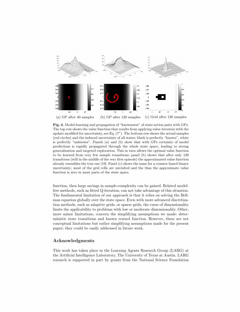
RMAXnoexp perform nearly the same. Initially, this appears to be in contrastwith the whole point of RMAX, which is efficient exploration guided by the un-certainty of the predictions. Here, we believe that this behavior can be explainedby the good generalization capabilities of GPs. Figure 4 illustrates model learn-ing and certainty propagation with GPs in the mountain car domain (predictingacceleration as function of state). The state of the model-learner is shown fortwo snapshots: after 40 transitions and after 120 transitions. The top row showsthe value function that results from applying value iteration with the updatemodified for uncertainty, see Eq. (7”). The bottom row shows the observed sam-ples and the associated certainty of the predictions. As expected, certainty ishigh in regions where data was observed. However, due to the generalizationof GPs and data-dependent hyperparameter selection, certainty is also high inunexplored regions; and in particular it is constant along the y-coordinate. Tounderstand this, we have to look at the state transition function of the moun-tain car: acceleration of the car indeed only depends on the position, but not onvelocity. This shows that certainty estimates of GPs are supervised and take theproperties of the target function into account, whereas prior RMAX treatmentsof uncertainty are unsupervised and only consider the density of samples to de-cide if a state is “known”. For comparison, we also show what GP-RMAX withgrid-based uncertainty would produce in the same situation.
5 Summary
We presented an implementation of model-based online reinforcement learningsimilar to RMAX for continuous domains by combining GP-based model learn-ing and value iteration on a grid. Doing so, our algorithm separates the problemfunction approximation in the model-learner from the problem function approx-imation/interpolation in the planner. If the transition function is easier to learn,i.e., requires only few samples relative to the representation of the optimal value

0 5 10 15 20100
150
200
250
300
350
400
450
500
Episodes
Ste
ps to g
oal (low
er
is b
etter)
Mountain car (GP−RMAX)
optimal
GP−RMAX exp
GP−RMAX noexp
GP−RMAX grid5
GP−RMAX grid10
0 200 400 600 800 1000100
150
200
250
300
350
400
450
500
Episodes
Ste
ps to g
oal (low
er
is b
etter)
Mountain car (Sarsa)
optimal
Sarsa(λ) Tilecoding 10
Sarsa(λ) Tilecoding 20
0 5 10 15 20−600
−500
−400
−300
−200
−100
0
Episodes
Tota
l re
ward
(hig
her
is b
etter)
Inverted pendulum (GP−RMAX)
optimal
GP−RMAX exp
GP−RMAX noexp
GP−RMAX grid5
GP−RMAX grid10
0 100 200 300 400 500−450
−400
−350
−300
−250
−200
−150
−100
−50
0
Episodes
Tota
l re
ward
(hig
her
is b
etter)
Inverted pendulum (Sarsa)
optimal
Sarsa(λ) Tilecoding 10
Sarsa(λ) Tilecoding 40
0 10 20 30 40 50−14
−12
−10
−8
−6
−4
−2
Episodes
Tota
l re
ward
(hig
her
is b
etter)
Bicycle balancing (GP−RMAX)
Bicycle not balanced
optimal
GP−RMAX exp
GP−RMAX noexp
GP−RMAX grid5
0 50 100 150 200 250−14
−12
−10
−8
−6
−4
−2
Episodes
Tota
l re
ward
(hig
her
is b
etter)
Bicycle balancing (Sarsa)
Bicycle not balanced
optimal
Sarsa(λ) Tilecoding 7
Sarsa(λ) Tilecoding 10
0 20 40 60 80 10050
100
150
200
250
300
350
400
450
500
Episodes
Ste
ps to g
oal (low
er
is b
etter)
Acrobot (GP−RMAX)
optimal**
GP−RMAX exp
GP−RMAX noexp
GP−RMAX grid5
0 100 200 300 400 50050
100
150
200
250
300
350
400
450
500
Episodes
Ste
ps to g
oal (low
er
is b
etter)
Acrobot (Sarsa)
optimal**
Sarsa(λ) Tilecoding 7
Sarsa(λ) Tilecoding 20
Fig. 3. Learning curves of our algorithm GP-RMAX (left column) and the standardmethod Sarsa(λ) with tile coding (right column) in the four benchmark domains. Eachcurve shows the online learning performance and plots the total reward as a function ofthe episode (and thus sample complexity). The black horizontal line denotes the bestpossible performance computed offline. Note the different scale of the x-axis betweenGP-RMAX and Sarsa.
−1
−0.5
0
0.5
−0.05
0
0.05
0
5
10
15
20
25
(a) GP after 40 samples
−1
−0.5
0
0.5
−0.05
0
0.05
20
40
60
80
(b) GP after 120 samples
−1
−0.5
0
0.5
−0.05
0
0.05
0
2
4
6
8
(c) Grid after 120 samples
Fig. 4. Model-learning and propagation of “knownness” of state-action pairs with GPs.The top row shows the value function that results from applying value iteration with theupdate modified for uncertainty, see Eq. (7”). The bottom row shows the actual samples(red circles) and the induced uncertainty of all states: black is perfectly “known”, whiteis perfectly “unknown”. Panels (a) and (b) show that with GPs certainty of modelpredictions is rapidly propagated through the whole state space, leading to stronggeneralization and targeted exploration. This in turn allows the optimal value functionto be learned from very few sample transitions: panel (b) shows that after only 120transitions (still in the middle of the very first episode) the approximated value functionalready resembles the true one [19]. Panel (c) shows the same for a counter-based binaryuncertainty; most of the grid cells are unvisited and the thus the approximate valuefunction is zero in most parts of the state space.
function, then large savings in sample-complexity can be gained. Related model-free methods, such as fitted Q-iteration, can not take advantage of this situation.The fundamental limitation of our approach is that it relies on solving the Bell-man equation globally over the state space. Even with more advanced discretiza-tion methods, such as adaptive grids, or sparse grids, the curse of dimensionalitylimits the applicability to problems with low or moderate dimensionality. Other,more minor limitations, concern the simplifying assumptions we made: deter-ministic state transitions and known reward function. However, these are notconceptual limitations but rather simplifying assumptions made for the presentpaper; they could be easily addressed in future work.
Acknowledgments
This work has taken place in the Learning Agents Research Group (LARG) atthe Artificial Intelligence Laboratory, The University of Texas at Austin. LARGresearch is supported in part by grants from the National Science Foundation
(IIS-0917122), ONR (N00014-09-1-0658), DARPA (FA8650-08-C-7812), and theFederal Highway Administration (DTFH61-07-H-00030).
References
1. A. Bernstein and N. Shimkin. Adaptive-resolution reinforcement learningwith efficient exploration. Machine Learning (published online: 5 May 2010).DOI:10.1007/s10994-010-5186-7, 2010.
2. G. Boone. Minimum-time control of the acrobot. Proc. of IEEE InternationalConference on Robotics and Automation, 4:3281–3287, 1997.
3. R. Brafman and M. Tennenholtz. R-MAX, a general polynomial time algorithmfor near-optimal reinforcement learning. JMLR, 3:213–231, 2002.
4. L. Busoniu, D. Ernst, B. De Schutter, and R. Babuska. Online least-squares pol-icy iteration for reinforcement learning control. In American Control Conference(ACC-10), 2010.
5. S. Davies. Multidimensional triangulation and interpolation for reinforcementlearning. In NIPS 9. Morgan, 1996.
6. M. P. Deisenroth, C. E. Rasmussen, and J. Peters. Gaussian process dynamicprogramming. Neurocomputing, 72(7-9):1508–1524, 2009.
7. Y. Engel, S. Mannor, and R. Meir. Bayes meets Bellman: The Gaussian processapproach to temporal difference learning. In Proc. of ICML 20, pages 154–161,2003.
8. D. Ernst, P. Geurts, and L. Wehenkel. Tree-based batch mode reinforcement learn-ing. JMLR, 6:503–556, 2005.
9. L. Grune. An adaptive grid scheme for the discrete Hamilton-Jacobi-Bellmanequation. Numerische Mathematik, 75:319–337, 1997.
10. N. K. Jong and P. Stone. Model-based exploration in continuous state spaces. InThe 7th Symposium on Abstraction, Reformulation and Approximation, 2007.
11. T. Jung and D. Polani. Learning robocup-keepaway with kernels. JMLR: Workshopand Conference Proceedings (Gaussian Processes in Practice), 1:33–57, 2007.
12. M. G. Lagoudakis and R. Parr. Least-squares policy iteration. JMLR, 4:1107–1149,2003.
13. L. Li, M. L. Littman, and C. R. Mansley. Online exploration in least-squares policyiteration. In Proc. of 8th AAMAS, 2009.
14. R. Munos and A. Moore. Variable resolution discretization in optimal control.Machine Learning, 49:291–323, 2002.
15. A. Nouri and M. L. Littman. Multi-resolution exploration in continuous spaces.In NIPS 21, 2008.
16. J. Quinonero-Candela, C. E. Rasmussen, and C. K. I. Williams. Approximationmethods for gaussian process regression. In Leon Bottou, Olivier Chapelle, DennisDeCoste, and Jason Weston, editors, Large Scale Learning Machines, pages 203–223. MIT Press, 2007.
17. C. E. Rasmussen and C. K. I. Williams. Gaussian Processes for Machine Learning.MIT Press, 2006.
18. M. Riedmiller. Neural fitted q-iteration. In Proc. of 16th ECML, 2005.19. R. Sutton and A. Barto. Reinforcement Learning: An Introduction. MIT Press,
1998.