ecm-cointegration test with garch(1,1)...
TRANSCRIPT

1
ECM-Cointegration test with GARCH(1,1) Errors.
Panagiotis Mantalos
Department of Science and Health Blekinge Institute of Technology
Sweden
ABSTRACT
By using Monte Carlo experiment, we study the robustness of the ECM-Cointegration tests when the first difference of the series follow a GARCH(1,1) process and the behaviour of the ARCH-tests of ECM residuals for variation of GARCH parameters. We found that if two series are individually I(1) and follow a GARCH (1,1), then ECM-Cointegration test tend to overreject for small samples but the problem is not very serious for large sample except when the errors´s GARCH process is nearly integrated and the volatility parameter is not small. Finally the Wild Bootstrap is robust on GARCH(1,1) without lost of power.
Keywords: ARCH, Bootstrap, Cointegration, GARCH, Wild Bootstrap.
Communications should be sent to: Panagiotis Mantalos, Department of Science and Health, Blekinge Institute of Technology, 371 79 Karlskrona, Sweden. E-mail : [email protected]
2
1. Introduction
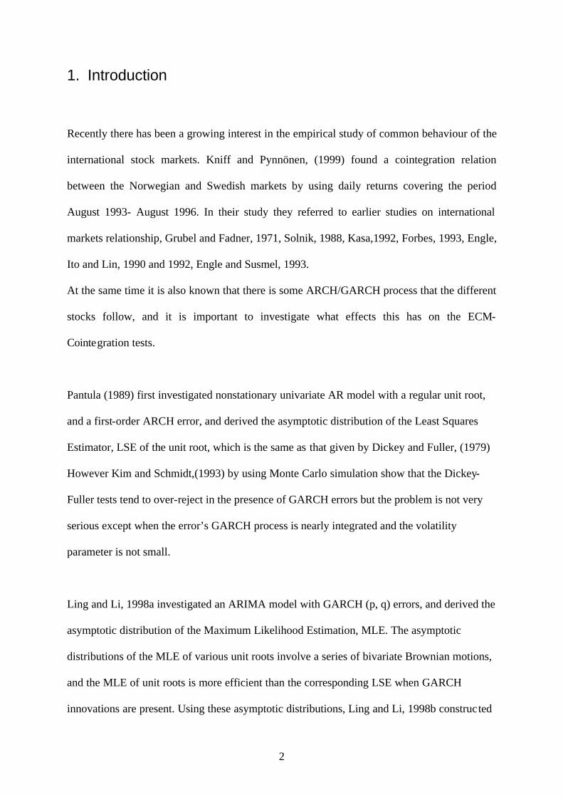
Recently there has been a growing interest in the empirical study of common behaviour of the
international stock markets. Kniff and Pynnönen, (1999) found a cointegration relation
between the Norwegian and Swedish markets by using daily returns covering the period
August 1993- August 1996. In their study they referred to earlier studies on international
markets relationship, Grubel and Fadner, 1971, Solnik, 1988, Kasa,1992, Forbes, 1993, Engle,
Ito and Lin, 1990 and 1992, Engle and Susmel, 1993.
At the same time it is also known that there is some ARCH/GARCH process that the different
stocks follow, and it is important to investigate what effects this has on the ECM-
Cointegration tests.
Pantula (1989) first investigated nonstationary univariate AR model with a regular unit root,
and a first-order ARCH error, and derived the asymptotic distribution of the Least Squares
Estimator, LSE of the unit root, which is the same as that given by Dickey and Fuller, (1979)
However Kim and Schmidt,(1993) by using Monte Carlo simulation show that the Dickey-
Fuller tests tend to over-reject in the presence of GARCH errors but the problem is not very
serious except when the error’s GARCH process is nearly integrated and the volatility
parameter is not small.
Ling and Li, 1998a investigated an ARIMA model with GARCH (p, q) errors, and derived the
asymptotic distribution of the Maximum Likelihood Estimation, MLE. The asymptotic
distributions of the MLE of various unit roots involve a series of bivariate Brownian motions,
and the MLE of unit roots is more efficient than the corresponding LSE when GARCH
innovations are present. Using these asymptotic distributions, Ling and Li, 1998b constructed
3
some new unit root tests, and show by using Monte Carlo simulation, that the new tests can
have a better performance than the Dickey-Fuller tests.
In the cointegration case Hansen and Rahbek (1999) based on an operational drift criterion
from Markov chain theory, showed that Cointegration analysis of vector autoregressive
models is robust with respect to ARCH innovations.
Li, Ling and Wong (1998) by studying an m-dimensional autoregressive process with
GARCH(p,q) innovations, showed that the full rank and the reduced rank MLE are more
efficient than the LSE.
However, as the ECM procedure is a special case of Johansen’s procedure for a system in
which the Cointegrating vectors appear only in the equation of interest, KED suggested
analysing only the equation of interest as a conditional equation. And Mantalos (1999) in an
empirical investigation of the Cointegration relationship between French and German stock
markets, under period 1.11.1997- 31.3.1999 found that even when the series individually
follow a GARCH(1,1) (nearly integrated GARCH process with small volatility parameter ),
all the ARCH test showed that there is no ARCH in variance of the ”ECM-Cointegration tests
regressions” residuals.
That is, there is a need for study of the ECM-Cointegration tests in the presence of conditional
heteroskedasticity of the GARCH(1,1) form.
The purpose of this paper is to study the robustness of the ECM-Cointegration tests when the
first difference of the series follow a GARCH(1,1) process and the behaviour of the ARCH-
tests of ECM residuals nearly integrated GARCH process with small volatility parameter.
4
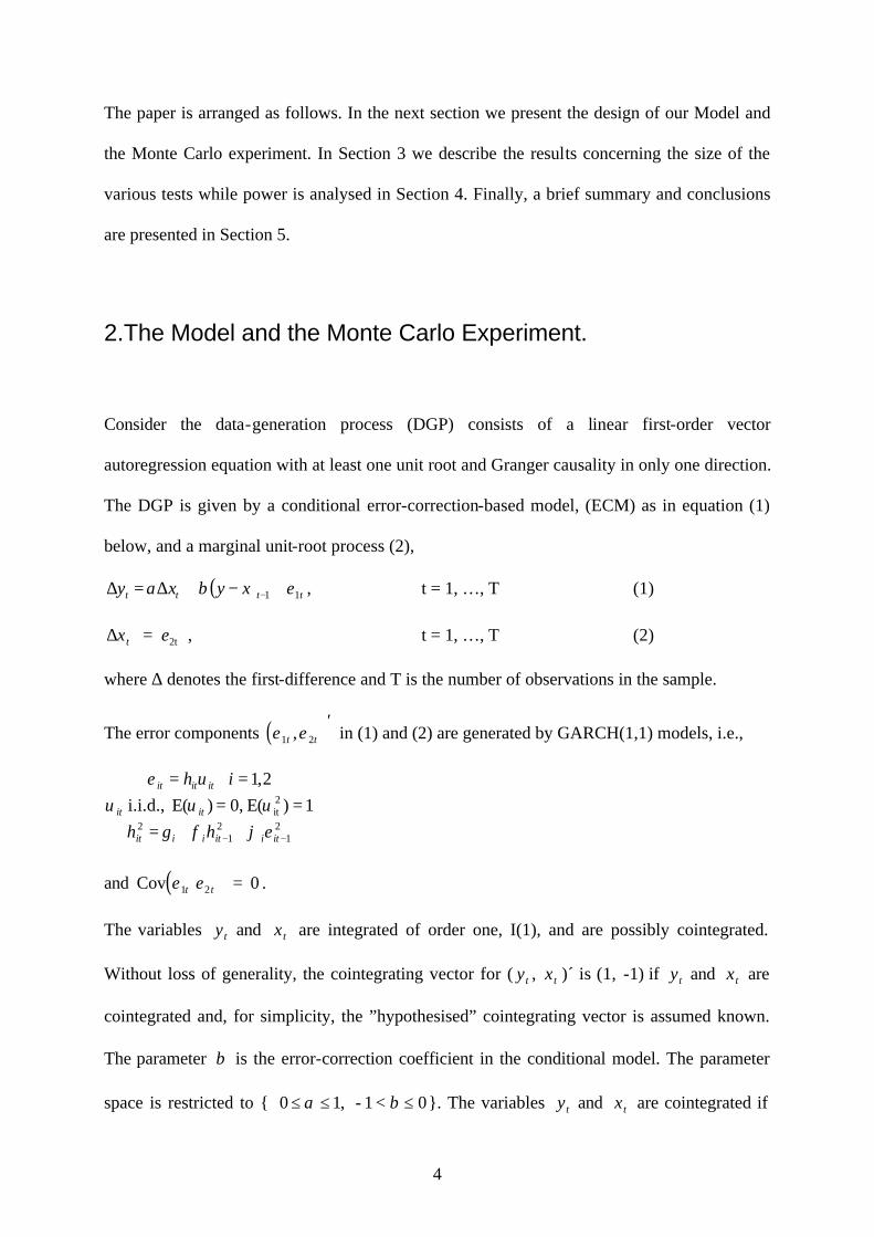
The paper is arranged as follows. In the next section we present the design of our Model and
the Monte Carlo experiment. In Section 3 we describe the results concerning the size of the
various tests while power is analysed in Section 4. Finally, a brief summary and conclusions
are presented in Section 5.
2.The Model and the Monte Carlo Experiment.
Consider the data-generation process (DGP) consists of a linear first-order vector
autoregression equation with at least one unit root and Granger causality in only one direction.
The DGP is given by a conditional error-correction-based model, (ECM) as in equation (1)
below, and a marginal unit-root process (2),
( ) tttt xyxy 11 = εβα +−+∆∆ − , t = 1, …, T (1)
∆x t 2t = ε , t = 1, …, T (2)
where ∆ denotes the first-difference and T is the number of observations in the sample.
The error components ( )ε ε1 2t t,′ in (1) and (2) are generated by GARCH(1,1) models, i.e.,
21
21
2
2it 1) E(0, ) E(i.i.d.,
2,1
−− ++===
==
itiitiiit
itit
ititit
hh
ih
εϕφγυυυ
υε
and ( )Cov = 0ε ε1 2t t .
The variables y t and x t are integrated of order one, I(1), and are possibly cointegrated.
Without loss of generality, the cointegrating vector for ( y t , x t )´ is (1, -1) if y t and x t are
cointegrated and, for simplicity, the ”hypothesised” cointegrating vector is assumed known.
The parameter β is the error-correction coefficient in the conditional model. The parameter
space is restricted to { 0 , - 1 < 0≤ ≤ ≤α β1 }. The variables y t and x t are cointegrated if

5
β < 0 , and non-cointegrated if β = 0 . Thus, in the ECM approach as in equation (1), the t-
ratio based upon the Least Squares (OLS) estimate β , denoted $βOLS , is the ECM statistic
(denoted TECM). That is, the estimated equation (1) is:
( ) tttt xyxy 11 ˆˆˆ = εβα +−+∆∆ − . (3)
The ECM statistic is TECM = $β / ese( $β ), where ese(.) denotes the estimated standard error
of its argument, to be used in testing the null hypothesis that β = 0 , i.e., that y t and x t are
not cointegrated.
The condition for finite variance is 1<+ ii ϕφ and the condition for finite fourth moment is
.123 221 <++ iiii ϕϕφφ And if 0>iγ and 1<+ ii ϕφ , then the unconditional variance of the
iε exist and equals ( )iiii ϕφγσ ε −−= 1/2 .
Note that when 0== ϕφ , the itε reduced to iid white noises.
In the case when the error components ( )ε ε1 2t t,′ in (1) and (2) are iid as bivariate normal
with ( ) ( ) ( )Ε Εε ε ε σ ε1 2 1 12
t t t = = 0 and Var = , ( )Var = ε σ ε2 22
t and ( )Cov = 0ε ε1 2t t ,
∀ t, studied by Kremers, Ericsson and Dolado (1992), KED.
KED examine the reason for the low power of the Dickey-Fuller test, (DF) and by using
Monte Carlo methods studied the small sample properties of two different versions of the
cointegration test, DF and ECM. KED found also by defining a ”signal-to-noise” ratio:
q = - (α -1)s, where s denote the ratio σ ε 2 / σ ε1 (assumed strictly positive), and q 2 is the
variance of ( )α −1 ∆x t relative to ε1t (see KED Section 3, p. 330) and using three different
sets of asymptotic critical values, that the size of the ECM tests is relative to q. That is, the
size of the ECM test in the KED study shows that there is a need for a set of robust critical
values.

6
One way to solve this problem and produce a set of robust critical values for ECM test is to
use bootstrap technique. Mantalos and Shukur (1998), MS, by using the same DGP as in
KED, improved the critical values of the ECM test statistic by employing residual based
bootstrap technique and they showed with Monte Carlo experiment that the size of the test
approaches its nominal value without loss of power. However here we use the Wild
Bootstrap, Wu (1986) that is robust against heteroskedasticity.
Before we describe our Monte Carlo Experiment we have to explain why we study the near
Integrated GARCH model that the residual from ECM model (3) follows.
Because the unconditional variance equal ( )iii ϕφγ −−1/ , one might expect that γ is close to
zero when ϕφ + is close to one, and vice versa, so that the unconditional variance is not too
large or too small.
Moreover as Kim and Schmidt (1993) point out in their study that Nelson (1990,1992)
considers GARCH model as an approximation to an underlying continuous-time diffusion
process. Letting L 0→ if the parameters follow the sequence:
φϕφωγ -1 and ,La , === L ,
with “ω ” and “a “ fixed. According to this result we might expected GARCH model applied
to high-frequency data to be nearly integrated and exhibit small values of γ and φ and finally
ϕ near unity.
Furthermore the ECM is an extension to Dickey-Fuller test for unit roots in system of
variables, and is interesting to compare the Kim and Schmidt (1993) results with our study.
And also because the GARCH model applied to stock market data, in Mantalos (1999) study,
was nearly integrated and exhibit small values of γ and φ and ϕ near unity.
The Monte Carlo experiment has been performed by generating data according to the model
defined by (1) and (2), we simulate also three near integrated GARCH with L equal to 0.25,

7
0.09 and 0.0064 and three GARCH with a) high persistence (0.01,0.09,0.9), b) medium
persistence (0,05, 0.05, 0.9) and c) low persistence (0.20,0,05,0.75).
We chose the parameter values, by fixing 1, = 22εσ and leaving the parameters
( 21εσ , ϕφγβα ,,, , ) and the sample size T as experimental design variables.
About the significance levels to be used when judging the properties of the tests, different
authors have put forward reasons for using both larger and smaller significance levels.
Maddala (1992) suggests using significance levels of as much as 25% in diagnostic testing,
while MacKinnon (1992) suggest going in the other direction.
To reduce this problem, in this study, we use mainly graphical methods that may provide
more information about the size and the power of the tests. We use simple graphical methods
that developed and illustrated by Davidson and MacKinnon (1997) and are easy to interpret,
the ”P value plot” to study the size and the ”Size-Power curves” to study the power of the
tests.
Furthermore to judge the reasonability of the results we use a 95% confidence interval for the
actual size (p) as : N
)1( 2 00
0
πππ −± , where N is the number of replications. Results that
lie between these bounds will be considered satisfactory.
For each time series 20 presample values are generated with zero initial conditions, taking net
sample sizes of T = 100, 500.
Tabel 1 shows the different parameters of our Monte Carlo design. The number of replications
per model is 10,000, for the size and 1000 for the power of the tests. The calculations were
performed using GAUSS 3.2.

8
Table 1 Monte Carlo Parameter Size
α
b γ φ ϕ 21ε
σ
Near Integrated 1/0.5 0 0.005 0.3 L ( )φγ −−1 1/16
High Persistence 1/0.5 0 0.01 0.09 0.90 1/16 Medium 1/0.5 0 0.05 0.05 0.90 1/16
Low 1/0.5 0 0.20 0.05 0.75 1/16
Power Near Integrated 1/0.5 0.02 0.005 0.3 L ( )φγ −−1 1/16
High Persistence 1/0.5 0.02 0.01 0.09 0.90 1/16 Medium 1/0.5 0.02 0.05 0.05 0.90 1/16
Low 1/0.5 0.02 0.20 0.05 0.75 1/16 Where L is 0.25, 0.09, 0.0064
The estimated equation (1) :
( ) tttt xyxy 11 ˆˆˆ = εβα +−+∆∆ − . (3)
and the ECM statistic TECM is used in testing the null hypothesis that β = 0 , i.e., that y t and
x t are not cointegrated.
The ARCH LM procedure test for autoregressive conditional heteroskedasticity (ARCH) is
used. And particularly the test is based on the regression of squared residuals from equation
(3) on one lagged, squared residuals and a constant.
The output from the test is a TR2 statistic, distributed as 2χ , with degrees of freedom equal to
the number of lagged, squared residuals, that is in our case one. Each statistic provides a test
of the hypothesis that the coefficients of the lagged squared residuals are all zero that is no
ARCH.
About our Bootstrap procedure we use the wild Bootstrap technique. A direct wild Bootstrap
gives:
** ˆˆ tttt uxy εα +∆=∆ (4)
to test if the variables are cointegrated. Where *tu are i.i.d observations drawn from some
distribution with c.d.f F, defined so as to satisfy:

9
.1)|( and 1)|( ,0)|( 3*2** === FuEFuEFuE ttT (5)
Let us denote by Ts the ECM test statistics, and by Ts* the ”Bootstrap test statistics”.
A Bootstrap estimate of the P-value for testing is P*{ Ts* ≥ Ts } and this approach we use to
examine the size of the Bootstrap test with the help of the ”P-value plot” .
The number of the Bootstrap sample used to estimate Bootstrap critical values and P-values in
our study is Νb = 199.
3.Results of the Size of the Tests
In this section we present the results of our Monte Carlo experiment concerning the sizes of
the tests.
Now for the P value plots, we have that if the distribution used to compute the ps is correct,
each of the ps should be distributed as uniform (0,1). Therefore the resulting graph should be
close to the 45o line i.e. as Figure 1a shows.
Figure 1 shows the ARCH LM test for different “L”, and we see that the test has the right size
for white noise residuals and has adequate power with ARCH parameter larger than 0,09.
Note also that the Figure 1a for ARCH parameter 0,024 shows that the power of the test is
very low and is almost equal to the size. This result explains why the ARCH tests in Mantalos
(1999) shows no ARCH effects on the ECM residuals. That is if two series are individually
I(1) and follow a GARCH(1,1) process that is nearly Integrated with the same GARCH
parameter and the small volatility parameter(<0,03), then the ARCH-tests show that there is
no ARCH effect on the least squares residual by regress the first difference of the series.

10
Figure 1 ARCH test with different L
Figure 1a White Noise
0,00 0,05 0,10 0,15 0,20 0,25
0,00
0,05
0,10
0,15
0,20
0,25
Nominal Size
Act
ual S
ize
Figure 1a L=0,0064
0,00 0,05 0,10 0,15 0,20 0,25
0,00
0,05
0,10
0,15
0,20
0,25
Nominal Size
Act
ual S
ize
Figure 1a L=0,09
0,00 0,05 0,10 0,15 0,20 0,25
0,00
0,08
0,16
0,24
0,32
0,40
Nominal Size
Act
ual S
ize
Figure 1a L=0,25
0,00 0,05 0,10 0,15 0,20 0,25
0,0
0,1
0,2
0,3
0,4
0,5
Nominal Size
Act
ual S
ize
Note that the whole lines for the figures are the approximate 95% confidence interval for actual size
Figure 2 shows some of the advantages of the P value plots, since they make easy to
distinguish between tests that work badly, and tests that work well. We see that in almost all
the cases, for large sample (500 observations), the ECM cointegration tests with least squares
estimation seems to be robust for GARCH innovations. However ECM test over-rejects the
null hypothesis for small sample. Note also in the near integrated case it is a tendency to over-
rejects null hypothesis even for large sample when the ARCH parameter is not small.

11
Figure 2: P Value Plots for ECM-Cointegration (GARCH innovations). Figure 2a: High Persistence GARCH
0,00 0,05 0,10 0,15 0,20 0,25
0,00
0,05
0,10
0,15
0,20
0,25
Nominal Size
100 Obs
500 Obs
Figure 2d: Near Integrated : L=0.25
0,00 0,05 0,10 0,15 0,20 0,25
0,00
0,05
0,10
0,15
0,20
0,25
Nominal Size
500 Obs
100 Obs
Figure 2b: Medium Persistence GARCH
0,00 0,05 0,10 0,15 0,20 0,25
0,00
0,05
0,10
0,15
0,20
0,25
Nominal Size
100 Obs
500 Obs
Figure 2e: Near Integrated : L=0.09
0,00 0,05 0,10 0,15 0,20 0,25
0,00
0,05
0,10
0,15
0,20
0,25
Nominal Size
100 Obs
500 Obs
Figure 2c: Low Persistence GARCH
0,00 0,05 0,10 0,15 0,20 0,25
0,00
0,05
0,10
0,15
0,20
0,25
Nominal Size
100 Obs
500 Obs
Figure 2f: Near Integrated : L=0.0064
0,00 0,05 0,10 0,15 0,20 0,25
0,00
0,05
0,10
0,15
0,20
0,25
Nominal Size
100 Obs
500 Obs
Note that the dot lines for the figures are the approximate 95% confidence interval for actual size

12
Figure 3: P Value Plots for ECM-Cointegration (GARCH innovations), q Effect.
Figure 3a: High Persistence GARCH
0,00 0,05 0,10 0,15 0,20 0,25
0,00
0,05
0,10
0,15
0,20
0,25
Nominal Size
Act
ual S
ize
q=0
q=2
Figure 2d: Near Integrated : L=0.25
0,00 0,05 0,10 0,15 0,20 0,25
0,00
0,05
0,10
0,15
0,20
0,25
Nominal Size
Act
ual S
ize
q=2
q=0
Figure 3b: Medium Persistence GARCH
0,00 0,05 0,10 0,15 0,20 0,25
0,00
0,05
0,10
0,15
0,20
0,25
Nominal Size
Act
ual S
ize
q=0
q=2
Figure 2e: Near Integrated : L=0.09
0,00 0,05 0,10 0,15 0,20 0,25
0,00
0,05
0,10
0,15
0,20
0,25
Nominal Size
Nom
inal
Siz
e
q=2
q=0
Figure 3c: Low Persistence GARCH
0,00 0,05 0,10 0,15 0,20 0,25
0,00
0,05
0,10
0,15
0,20
0,25
Nominal Size
Act
ual S
ize
q=2
q=0
Figure 2df Near Integrated : L=0.0064
0,00 0,05 0,10 0,15 0,20 0,25
0,00
0,05
0,10
0,15
0,20
0,25
Nominal Size
Actu
al S
ize
q=0
q=2
White noise q=2
Note that the dot lines for the figures are the approximate 95% confidence interval for actual size
Now, Figure 3 shows the combination of the GARCH and q effect on the ECM-cointegration
test. Remind the results from KED and MS studies; that for large q the ECM tests
systematically under-reject the null hypothesis. However, it seems to be a small tendency that
the over-reject from the GARCH effect to cancel the under-reject effect from large q, note
also that we q is only 2 in our experiment. Moreover the q effects it is obviously that dominate
over the GARCH effects.

13
By study the Figure 4, which shows the rejection of the tests on 5% nominal size, we can
summarise the results about the size of the tests, in our experiment.
Without q effect ECM cointegration test rejects about the right proportion of the time the null
hypothesis for large sample and for small ARCH parameter in near integrated case and over
reject for small sample even when there is low persistence effects.
With q=2 there is no large effect from the GARCH effects on ECM tests it seems that the q
effect dominates.
Figure 4. Comparison of The “q” and “GARCH” on 5% confidence interval
0,074
0,070
0,066
0,062
0,058
0,054
0,050
0,046
0,042
0,038
0,034
High Medium Low L=0,25 L=0,09 L=0,0064NoiseWhite
q=0 100 OBS
q=0 500 Obs
q=2 100 Obs
The Bootstrap test rejects about the right proportion of the time the null hypothesis, as Figure
5 shows, in the 95% confidence interval for both case without q effect and with q=2. Note that
we use only 100 Bootstrap-resample in our experiment more Bootstrap-resample makes the
line smooth without change the result.

14
Figure 5 Bootsttrap Test Figure 5a Bootstrap High
0,00 0,05 0,10 0,15 0,20 0,25
0,000
0,025
0,050
0,075
0,100
0,125
0,150
0,175
0,200
0,225
0,250
Nominal Size
Act
ual S
ize
q=2
q=1
Figure 5b Bootstrap Medium
0,00 0,05 0,10 0,15 0,20 0,25
0,000
0,025
0,050
0,075
0,100
0,125
0,150
0,175
0,200
0,225
0,250
Nominal Size
Act
ual S
ize
q=1
q=2
Figure 5c Bootstrap Low
0,00 0,05 0,10 0,15 0,20 0,25
0,000
0,025
0,050
0,075
0,100
0,125
0,150
0,175
0,200
0,225
0,250
Nominal Size
Act
ual S
ize
q=2
q=1

15
Finally, Figure 6 for 100 observations summarise all the above results for high, medium and
low persistence GARCH with or without q effects and results is that the wild Bootstrap is
robust. The ECM-cointegration test tend to over-reject in the presence of GARCH errors but
the problem is not very serious in large samples except when the error’s GARCH process is
nearly integrated and the volatility parameter is not small. And this result is the same with
Kim and Schmidt (1993) results.
Figure 5d: Near Integrated : L=0.25
0,00 0,05 0,10 0,15 0,20 0,25
0,000
0,025
0,050
0,075
0,100
0,125
0,150
0,175
0,200
0,225
0,250
Nominal Size
Act
ual S
ize q=1
q=2
Figure 5 f: Near Integrated : L=0.0064
0,00 0,05 0,10 0,15 0,20 0,25
0,000
0,025
0,050
0,075
0,100
0,125
0,150
0,175
0,200
0,225
0,250
Nominal Size
Act
ual S
ize
q=1
q=2
Figure 5e: Near Integrated : L=0.09
0,00 0,05 0,10 0,15 0,20 0,25
0,000
0,025
0,050
0,075
0,100
0,125
0,150
0,175
0,200
0,225
0,250
Nominal Size
Act
ual S
ize
q=2
q=1
Figure 5q: White noise
0,00 0,05 0,10 0,15 0,20 0,25
0,000
0,025
0,050
0,075
0,1000,125
0,150
0,1750,200
0,2250,250
Nominal Size
Act
ual S
ize
q=2
q=1

16
Figure 6. Comparison of The “q” and “GARCH” on 5% confidence interval
High Medium Low L=0,25 L=0,9 L=0,0064 Whitenoise
0,034
0,038
0,042
0,046
0,050
0,054
0,058
0,062
0,066
0,070
0,074
Index
Siz
e
q=1
q=2
Bot q=1
Bot q=2
4. Analysis of the Power of the Tests
In this section we discuss the most interesting results of our Monte Carlo experiment,
designed to gather evidence concerning the power of the various test versions. We analysed
the power of the ECM tests using sample sizes of, 100, and 500 observations and Bootstrap
tests using sample sizes of, 100, observations. The power function is estimated by calculating
the rejection frequencies in 1000 replications using values of the β coefficients = 0,2. The
estimated power functions of the tests have been compared only graphically as in the size
case. We use the Size-Power Curves to compare the power of alternative test statistics. This
has proved to be quite adequate, since the tests that gave reasonable results as regard size
usually differed very little regarding power. We follow the same procedure as for the size
investigation to evaluate the EDF’s denoted ( )$F x j⊕ , by using the same sequence of random
numbers as the one that we used to estimate the size of the tests.
Plotting the estimated power functions against the nominal size, we have the Size-Power
Curves. Note that the Size-Power Curves on a correct size-adjusted basis i.e plotting the
estimated power functions against the true size, that is ( )$F x j⊕ against ( )$F x j , do not show
much different than the standard Size-Power Curves and we do not show here.

17
Figure 7 Power –Size Plots of the ECM Test Figure 7a Power of High Persistence
0,0 0,2 0,4 0,6 0,8 1,0
0,0
0,2
0,4
0,6
0,8
1,0
Nominal Size
Pow
er
100 Obs
500 Obs
Figure 7d Power with L=0,25
0,0 0,2 0,4 0,6 0,8 1,0
0,0
0,2
0,4
0,6
0,8
1,0
Nominal Size
Pow
er 100 Obs
500 Obs
Figure 7b Power of Medium Persistence
0,0 0,2 0,4 0,6 0,8 1,0
0,0
0,2
0,4
0,6
0,8
1,0
Nominal Size
Pow
er 100 Obs
500 Obs
Figure 7e Power with L=0,09
0,0 0,2 0,4 0,6 0,8 1,0
0,0
0,2
0,4
0,6
0,8
1,0
Nominal Size
Pow
er W
N 5
00
100 Obs
500 Obs
Figure 7c Power of Low Persistence
0,0 0,2 0,4 0,6 0,8 1,0
0,0
0,2
0,4
0,6
0,8
1,0
Nominal Size
Pow
er
100 Obs
500 Obs
Figure 7f Power with L=0,0064
0,0 0,2 0,4 0,6 0,8 1,0
0,0
0,2
0,4
0,6
0,8
1,0
Nominal Size
Pow
er
100 Obs
500 Obs
18
Figure 7 presents the Size-Power Curves for the tests for different GARCH models in all
cases we see that it is a sample effect, higher power with large sample. We do not notice any
GARCH effect (solid line is the White noise model).
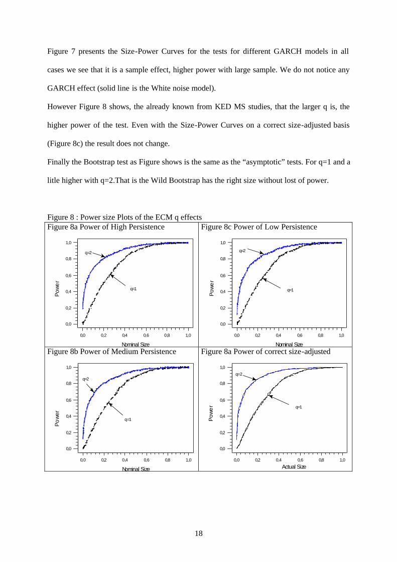
However Figure 8 shows, the already known from KED MS studies, that the larger q is, the
higher power of the test. Even with the Size-Power Curves on a correct size-adjusted basis
(Figure 8c) the result does not change.
Finally the Bootstrap test as Figure shows is the same as the “asymptotic” tests. For q=1 and a
litle higher with q=2.That is the Wild Bootstrap has the right size without lost of power.
Figure 8 : Power size Plots of the ECM q effects Figure 8a Power of High Persistence
0,0 0,2 0,4 0,6 0,8 1,0
0,0
0,2
0,4
0,6
0,8
1,0
Nominal Size
Pow
er
q=1
q=2
Figure 8c Power of Low Persistence
0,0 0,2 0,4 0,6 0,8 1,0
0,0
0,2
0,4
0,6
0,8
1,0
Nominal Size
Pow
er
q=1
q=2
Figure 8b Power of Medium Persistence
0,0 0,2 0,4 0,6 0,8 1,0
0,0
0,2
0,4
0,6
0,8
1,0
Nominal Size
Po
wer
q=1
q=2
Figure 8a Power of correct size-adjusted
0,0 0,2 0,4 0,6 0,8 1,0
0,0
0,2
0,4
0,6
0,8
1,0
Actual Size
Pow
er q=1
q=2

19
Figure 9 Bootstrap Power size Plots of the ECM
Bootstrap q=1
0,0 0,2 0,4 0,6 0,8 1,0
0,0
0,2
0,4
0,6
0,8
1,0
Nominal Size
Pow
er Bootstrap
Bootstrap q=2
0,0 0,2 0,4 0,6 0,8 1,0
0,0
0,2
0,4
0,6
0,8
1,0
Nominal Size
Pow
er Bootstrap
white noise
5. Summary and conclusions
By using Monte Carlo experiment, we study the robustness of the ECM-Cointegration tests
when the first difference of the series follow a GARCH(1,1) process and the behaviour of the
ARCH-tests of ECM residuals for variation of GARCH parameters. We defining a ”signal-to-
noise” ratio: q = - (α -1)s, where s denote the ratio σ ε 2 / σ ε1 (assumed strictly positive),
and q 2 is the variance of ( )α −1 ∆x t relative to ε1t (see Section 2).
We use simple graphical methods that developed and illustrated by Davidson and MacKinnon
(1997) and are easy to interpret, the ”P value plot” to study the size and the ”Size-Power
curves” to study the power of the tests.
Without q effect ECM cointegration test rejects about the right proportion of the time the null
hypothesis for large sample and for small ARCH parameter in near integrated case and over
reject for small sample even when there is low persistence effects.

20
With q=2 there is no large effect from the GARCH effects on ECM tests it seems that the q
effect dominates.
The Bootstrap test rejects about the right proportion of the time the null hypothesis, as Figure
5 shows, in the 95% confidence interval for both case without q effect and with q=2.
About the power of the tests the Size-Power Curves for different GARCH models in all cases
shows that there is a sample effect, higher power with large sample. We do not notice any
GARCH effect .
However Fig the Size-Power Curves show, the already known from KED MS studies, that the
larger q is, the higher power of the test. Even with the Size-Power Curves on a correct size-
adjusted basis (Figure 8c) the result does not change.
Finally the Bootstrap test as Figure shows is the same as the “asymptotic” tests. For q=1 and a
litle higher with q=2.
That is the Wild Bootstrap has the right size without lost of power.

21
References
Davidson, R and J.G. MacKinnon (1997): “ Graphical Methods for Investigating the Size and Power of Hypothesis Tests,” Working Paper, Department of Economics, University of Queen’s, Canada. Dickey, D. A, and Fuller W.A (1979): “ Distribution of the Estimators for Autoregressive Time Series with a Unit Root.” J.Amer.Statist. Assoc. 74, 427-431. Engle, Robert, F., and Susmel, Raul. (1993): “Common volatility in informational equity markets.” Journal of Business & Economic Statistics, 11. N0 2, 167-176. Engle, Robert, F., Tatkatoshi Ito, and Wen-Ling Lin (1990). “Meteor shower or heat waves? Intra-daily volatility in the foreign exchange market.” Econometrica, 58, No. 3, 525-542. Engle, Robert, F., Tatkatoshi Ito, and Wen-Ling Lin (1992): “Where does the meteor shower come from?. The role of stochastic policy coordination.” Journal of International Economics 32, 221-240. Forbes, William, P. (1993): “ The integration of European stock markets: The case of the banks.” Journal of Bisiness Finance & Acounting, 20, No 3, 427-439. Grubel, H.G., and K. Fadner (1971): “ The inteterdependence of international equity markets.” Journal of Finance XXVI, 89-94. Hansen, E and Rahbek, A. (1999): “ Stationarity and asymptotics of multivariate ARCH time series with an application to robustness of cointegration analysis. “ Technical report. Department of Theoretical Statistics University of Copenhagen Kasa, K. (1992): “ Common stochastic trends in international stock markets.” Journal of Monetary Economics, 29,95-124. Kim, K and Schmidt, P (1993): “ Unit Root Tests with Conditional Heteroskedasticity.” J. Econometrics 59, 287-300. Knif J and S. Pynnönen (1999): “ Local and global price memory of international stock markets. “ Journal of Inter. Financial Markets, Institutions & Money Vol. 9(2)129-147 Kremers, J. J. M., Ericsson, N. R. and Dolado, J. J. (1992) :” The power of Cointegration Tests.” Oxford Bullettin of Economics and Statistics, 54: 325-346. Li, W.K, Ling, S. And Wong, H. (1998): “ Estimation for Partially Nonstationary Multivariate Autoregressive Models with Conditional Heteroskedasticity.” Technical report. Department of Statistics, University of Hong Kong. Ling, S and Li, W.K (1998a): “Limiting Distributions of Maximum Likelihood Estimators for Unstable ARMA Models with GARCH Errors.” Ann.Statist. 26, 84-125
22
Ling, S and Li, W.K (1998b): “Estimation and Testing for Unit Root Processes with GARCH(1,1) Errors.” Technical report. Department of Statistics, University of Hong Kong. MacKinnon, J. G (1992): “ Model Specification Tests and Artificial Regressions, ” Journal of Economic Literature, 30, 102-146.” Maddala, G. S. (1992): Introduction to Econometrics, Second Edition, New York, Maxwell Macmillan. Mantalos, P (1999): “An Investigation of the Cointegration and Granger-cause Relationship Between French and German Stock Markets. Under Period 1.11.1997- 31.3.1999.” Technical report. Department of Statistics, University of Lund. Mantalos, P. and G. Shukur (1998): “ Size and Power of the Error Correction Model (ECM) Cointegration Test- A Bootstrap Approach, ” Oxford Bulletin of Economics and Statistics : Vol 60 (1998). Nelson, D. B (1990) : “Stationary and Persistence in the GARCH(1,1) Model.” Econometric Theory 6:318-34. Pantula, S.G. (1989): “ Estimation of Autoregressive Models with ARCH Errors. “ Sankhya B, 50, 119-138 Solnik, B.(1988) International Investments. Addinson-Wesley, United States. Wu, C.F.J. (1986): “Jackknife, bootstrap and other resampling methods in regression analysis, Ann.Statist., 14, 1261-1350