eco-efficiency and convergence in oecd countries
TRANSCRIPT
Environ Resource Econ (2013) 55:87–106DOI 10.1007/s10640-012-9616-9
Eco-Efficiency and Convergence in OECD Countries
Mariam Camarero · Juana Castillo ·Andrés J. Picazo-Tadeo · Cecilio Tamarit
Accepted: 6 November 2012 / Published online: 19 November 2012© Springer Science+Business Media Dordrecht 2012
Abstract This paper assesses the convergence in eco-efficiency of a group of 22 OECDcountries over the period 1980–2008. In doing so, three air pollutants representing the impacton the environment of economic activities are considered, namely, carbon dioxide (CO2),nitrogen oxides (NOX) and sulphur oxides (SOX); furthermore, eco-efficiency scores atboth country and air-pollutant-specific level are computed using Data Envelopment Analysistechniques. Then, convergence is evaluated using the recent approach by Phillips and SulEconometrica 75:1771–1855 (2007), which tests for the existence of convergence groups.First, we find that eco-efficiency has improved over the period, with the exception of NOX
emissions. Second, Switzerland is the most eco-efficient country, followed by some Scan-dinavian economies, such as Sweden, Iceland, Norway and Denmark. In contrast, SouthernEuropean countries such as Portugal, Spain and Greece, in addition to Hungary, Turkey,Canada and the United States, are among the worst performers. Finally, we find that both themost eco-efficient countries and the worst tend to form clubs of convergence.
Keywords Air pollutants · Eco-efficiency · Data Envelopment Analysis ·Convergence clubs · OECD
JEL classification C15 · C22 · C61 · F15 · Q56
1 Introduction
The concept of economic and ecological efficiency, more popularly known as eco-efficiency,emerged in the nineties as a practical approach to the more encompassing notion of sus-tainability (Schaltegger 1996). The OECD provided a broad definition of eco-efficiency as
M. CamareroDpto. Economía, Universidad Jaume I, Campus del Riu Sec, 12071 Castellón, Spain
J. Castillo · A. J. Picazo-Tadeo (B)· C. TamaritDpto. Economía Aplicada II, Universidad de Valencia, Campus de Tarongers, 46022 Valencia, Spaine-mail: [email protected]
123
88 M. Camarero et al.
‘the efficiency with which ecological resources are used to meet human needs’ (OECD 1998)and the concept was afterwards popularised by the World Business Council for SustainableDevelopment (WBCSD 2000). More specifically, eco-efficiency refers to the ability of firms,industries, regions or economies to produce more goods and services with fewer impacts onthe environment and less consumption of natural resources, thus bringing together economicand ecological issues. Furthermore, in recent years, firm managers, researchers and policy-makers are paying particular attention to the issue of eco-efficiency. While firms have realisedthat taking the lead in environmental behaviour could give them a competitive advantage(Porter and van der Linde 1995), researchers face the challenge of providing policymak-ers with sound information to improve the design of their environmental policies aimed atupholding longer-term sustainability.
Eco-efficiency starts at firm level with recommendations to reduce material requirements,the energy intensity of commodities and services, toxic dispersion and to maximise thesustainable use of renewable resources (WBCSD 2000). However, as human societies aspireto satisfy increasing levels of consumption and the simultaneous attainment of reasonableenvironmental quality, the eco-efficiency concept should be extended to an economy-wideand macro-level beyond the business sector and production patterns (United Nations 2009).Likewise, environmental policies aimed at boosting eco-efficiency at micro level are relevantfor improving firms’ competitiveness, but do not necessarily guarantee sustainability.
The indicators created to implement the notion of eco-efficiency are based on ratios thatrelate the economic value of goods and services produced to the environmental pressuresor impacts involved in production processes, the larger the ratio the higher the level of eco-efficiency attained (see Schmidheiny and Zorraquin 1996; Figge and Hahn 2004; Huppesand Ishikawa 2005). The literature in this field of research suggests different approaches tothis eco-efficiency ratio depending on factors such as the scale of the analysis, the adoptionof a short or a long-term perspective and the broadness of scope in the definition of botheconomic value and environmental impact.
The assessment of eco-efficiency was initially approached by simple indicators, such asGDP over CO2 at macro-level or units of output per unit of waste or environmental pressure atmicro-level. The main advantage of these indicators is that they can be easily understood bypolicymakers as well as by the general public. However, in spite of their straightforwardness,these simple indicators have significant shortcomings, ignoring, for example, that a giveneconomic value can be obtained with different combinations of pressures or impacts onthe environment. Instead, more sophisticated approaches to assessing eco-efficiency havebeen developed in recent years, including benchmarking techniques in the framework ofconventional efficiency analysis.
In this context, the aim of our paper is to analyse the degree of eco-efficiency convergencein 22 OECD countries during the period 1980–2008. In a first stage, we assess eco-efficiencyusing the recent proposal by Picazo-Tadeo et al. (2011) and Data Envelopment Analysis(DEA) techniques or activity models, which make it possible to incorporate several envi-ronmental pressures as well as to assess eco-efficiency at specific environmental pressurelevel. Furthermore, we focus on three air pollutants because of their transnational impor-tance and cross-border nature, namely, carbon dioxide (CO2), nitrogen oxides (NOX) andsulphur oxides (SOX). Secondly, we study convergence in eco-efficiency making use of themethodological approach proposed by Phillips and Sul (2007), which tests for the existenceof convergence clubs. This approach studies relative convergence which is especially suitedto the case of efficiency, also defined in relative terms.
Convergence in air emissions is at present a core concern for policymakers. This is amatter of particular importance in developed countries that are currently working towards
123
Eco-Efficiency and Convergence in OECD Countries 89
the long-run objective of achieving a fair distribution of emission among countries. As notedby Westerlund and Basher (2008), ‘… For this to happen evidence of convergence is a must,while lack of emissions convergence may protract the process of emissions allocation tomaterialize’. Convergence in developed economies should also be a good example to followfor developing countries, facilitating the fulfilment of their commitments of abating pollution.Moreover, projections on air emissions carried out by international organisations are mostlybased on the assumption of convergence (IPCC 2007).
Several papers have analysed convergence in emissions using variables such as per capitaCO2 emissions (representative papers include Lanne and Liski 2004; Aldy 2006, 2007;Ezcurra 2007; Westerlund and Basher 2008; Romero-Ávila 2008; Lee and Chang 2008,2009; Barassi et al. 2008, 2011; Jobert et al. 2010; Ordás Criado and Grether 2011) or,in fewer cases, CO2 emissions over GDP (Camarero et al. 2013). However, most of thesestudies have only accounted for the environmental side of production processes, i.e., analysesbased on variables such as per capita emissions, and/or they have only considered a singleemission to represent the impact of economic activity on the environment. In our opinion,the joint use of a DEA-based assessment of eco-efficiency with the Phillips and Sul (2007)approach to convergence might provide new insights into this burgeoning literature in thefield of emission convergence.
Firstly, eco-efficiency indicators based on activity models account not only for the envi-ronmental side of production processes but also for economic issues, thus providing a morecomprehensive view of the relationship between the economy and the environment. Sec-ondly, beyond simple indicators considering a single emission, by using activity models wecan obtain indicators of eco-efficiency that account simultaneously for several emissions orpressures exerted by production processes on the environment; moreover, performance canbe assessed at the level of specific environmental emissions. To the best of our knowledge,no previous paper has analysed convergence in eco-efficiency using composite indicatorsof environmental performance.1,2 In the third place, unlike most previous research in thefield of environmental convergence, the approach by Phillips and Sul (2007) used in thispaper identifies groups of countries that converge to different equilibria, allowing individualcountries to diverge.3
Accordingly, analysing emission convergence with DEA-based indicators that considerjointly both ecological and economic aspects of production processes as well as severalemissions on the environment could provide policymakers with useful information that goesbeyond the results of more conventional convergence analyses based on ratios such as emis-sions of single pollutants per capita or emissions over GDP. Moreover, results from renewedapproaches to convergence assessment might help policymakers to design more effective reg-
1 Camarero et al. (2008) tested for convergence in the environmental performance of 22 OECD countries duringthe period 1970–2002 using a series of indicators computed within the framework of the production theory. Inaddition, Nourry (2009) analysed the hypothesis of stochastic convergence for CO2 and SO2 emissions usinga pair-wise approach that considers all the pairs of per capita gas emission gaps across a sample of 127 and81 countries for carbon dioxide and sulfur dioxide, respectively.2 Furthermore, although some recent papers such as Zhang et al. (2008) and Wursthorn et al. (2011) haveassessed eco-efficiency using aggregate data at sector or regional level, no previous paper has addressed, tothe best of our knowledge, the assessment of eco-efficiency at pressure-specific and country level, as we doin our paper. Only Kortelainen (2008) constructed a dynamic environmental performance index based on thestandard definition of eco-efficiency at macro-level for 20 European Union members.3 Only a few papers have used this approach to convergence assessment in the field of environmental studies.Panopoulou and Pantelidis (2009) explains club convergence in per capita CO2 emissions among 128 countriesin 1960–2003; Camarero et al. (2013) studies convergence among OECD countries in 1960–2008 in CO2emission intensity and its determinants, namely, energy intensity and the so-called carbonisation index.
123
90 M. Camarero et al.
ulations on air pollution, which are the most important environmental policies in developedcountries. In addition, some light might be shed on relevant questions such as: Has the eco-efficiency of developed countries improved since the eighties? If so, are there differences ineco-efficiency depending on the management of different pollutants? Have developed coun-tries achieved eco-efficiency convergence? If this is the case, have some countries sharedcommon convergence patterns, thus forming convergence clubs? Are differences in conver-gence paths according to pollutants important?
Following this Introduction, Sect. 2 describes the data and sources of information andexpounds the main insights of the methodology. Section 3 discusses the results and a finalsection summarises and concludes.
2 Data and Methodological Issues
2.1 Data and Sources of Information
In this paper, we use a dataset of 22 OECD countries that covers the period 1980–2008.4
These countries are: Austria (Aus), Belgium (Bel), Canada (Can), Denmark (Dnk), Finland(Fin), France (Fra), Germany (Deu), Greece (Grc), Hungary (Hun), Iceland (Isl), Ireland(Ire), Italy (Ita), Luxembourg (Lux), Netherlands (Nld), Norway (Nor), Portugal (Prt),Spain (Esp), Sweden (Swe), Switzerland (Che), Turkey (Tur), the United Kingdom (GBr)and, finally, the United States (USA).
The economic value of the goods and services produced by these countries, i.e., theireconomic performance, is measured by real GDP in constant dollars (millions US$, baseyear 2000), with data from the World Bank.5 Concerning ecological performance, as alreadynoted, three air pollutants are considered, namely, CO2 emissions, NOX emissions and SOX
emissions, all measured in Kt. These pollutants account for nearly 80 % of total air pollution.Carbon dioxide is mostly released through the combustion of fossil fuels and is by far thelargest contributor to worsening greenhouse effects.6 Nitrogen and sulphur oxides also con-tribute to global warming and generate acid rain that affects forests, agriculture and fishing.Data on CO2 emissions come from the World Bank, while data on NOX and SOX emissionshave been obtained from the Centre on Emission Inventories and Projections (CEIP) hostedby the Austrian Environment Agency.7
2.2 Computing Specific Environmental Pressure Scores of Eco-Efficiency
We assess eco-efficiency using the proposal by Picazo-Tadeo et al. (2011) based on previouswork by Torgersen et al. (1996) and Kuosmanen and Kortelainen (2005). This provides the
4 The extent of our dataset regarding both countries included and years is determined by the availability ofstatistical information.5 Accessed through http://databank.worldbank.org.6 The Intergovernmental Panel on Climate Change considers carbon dioxide to be responsible for more thansixty percent of the global warming expected in the twentyfirst century (IPCC 1990).7 The CEIP (http://www.ceip.at) provides official data on air-pollution emissions, as well as the data usedin the models of the European Monitoring and Evaluation Programme (EMEP, http://www.emep.int). Whilethe former are directly reported for individual countries, the latter are harmonised by the CEIP. This is whyharmonised data are strongly recommended for modelling and cross-country comparisons. The EMEP seriesinclude data on air pollutants for 1980 and 1985 and annual data from 1990 onwards. Conversely, officialreported data start in 1980. We have completed the series of harmonised data for the 1980s by applying thegrowth rates of official data to harmonised data from 1980 and 1985. These series are available upon request.Finally, the data for Canada and the United States are the original officially reported data.
123
Eco-Efficiency and Convergence in OECD Countries 91
basis to compute scores of overall eco-efficiency for the developed countries in our sample,but also the scores of eco-efficiency in terms of the emission of each particular air pollutant.
Therefore, let g be the observed GDP of each OECD country c = 1, . . . , 22 in the sample.Moreover, we also observe the volume of CO2, NOX and SOX emissions that exert a series ofpressures on the environment represented by the vector p = (
pC O2 , pN OX , pSOX
). The Pres-
sure Generating Technology set (PGT) indicating all the feasible combinations of GDP andenvironmental pressures is (see Kuosmanen and Kortelainen 2005; Picazo-Tadeo et al. 2011):
PGT =[(g, p) ∈ R1+3+ | GDP g can be generated with environmental pressures p
](1)
Next, we borrow the definition of eco-efficiency from Kuosmanen and Kortelainen (2005) asthe ratio between an indicator of economic performance, measured in our case by GDP, and anaggregate environmental pressure composite indicator. This ratio is defined for country co as:
Eco − efficiencyco= GDPco
Aggregate environmental pressureco
= gco
F(
pco
) = gco
wC O2co pC O2co +wN OX co pN OX co + wSOX co pSOX co
(2)
where F is a function that aggregates the pressures exerted on the environment by the threeair-polluting gases into a single environmental pressure score, whereas wC O2co , wN OX co andwSOX co are the weights assigned to CO2, NOX and SOX emissions in computing the aggre-gate pressure.
As in Picazo-Tadeo et al. (2011), eco-efficiency is assessed using Data EnvelopmentAnalysis (DEA), which is a well-known non-parametric approach to efficiency measurementpioneered by Charnes et al. (1978). This technique uses mathematical programming to con-struct, on the basis of observed data, a technological frontier representing the best practicesand then compares particular observations to the frontier in order to obtain a measure of theirrelative performance (see Cooper et al. 2007 for the foundations of DEA).8 One practicaladvantage of DEA is that the weights that individual emissions are assigned for the compu-tation of the aggregate environmental pressure score involved in the denominator of the ratioof eco-efficiency in expression (2) are determined endogenously at country level, allowingfor the possibility of substitution between environmental pressures.9 Formally, the indicatorof overall eco-efficiency for country co is computed using the following program:10
Minimize φco , zc Eco − efficiencyco = φco
subject to:
gco ≤22∑
c=1zc · gc (i)
φco · pnco ≥22∑
c=1zc · pnc n = CO2, NOX and SOX (i i)
zc ≥ 0 c = 1, . . . , 22 (i i i)
(3)
8 DEA has been widely used for the analysis of environmental performance; Zhou et al. (2008) review theempirical applications of these techniques in energy and environmental studies.9 The weight assigned to each environmental pressure is calculated in such a way that it rates each countryin the most favourable light in relation to all the other countries in the sample when those same weights areused. Nonetheless, as pointed out by Kuosmanen and Kortelainen (2005), additional a priori restrictions onthe relative importance of environmental pressures could also be accounted for (Allen and Thanassoulis 2004review the techniques used to introduce these weight restrictions in DEA).10 Constant returns to scale are assumed in this program; Kuosmanen and Kortelainen (2005) and Picazo-Tadeo et al. (2011) justify this assumption.
123

92 M. Camarero et al.
where zc is a set of intensity variables which represents the weights assigned to each observedcountry c in the construction of the eco-efficient frontier.
The parameter obtained as the solution to program (3) measures the amount by whichcountry co could proportionally reduce CO2, NOX and SOX emissions without decreasingits GDP and is upper-bounded to one, the score that represents the best performance. More-over, the lower the score, the worse the level of eco-efficiency; e.g., a score of, say, 0.7would mean that all three emissions could be decreased by 30 % while maintaining GDP.Making a parallelism with conventional literature on DEA, this parameter would measureeco-efficiency in a Farrell-Debreu sense (Farrell 1957). Nonetheless, once the greatest radialor proportional reduction in emissions of our three air pollutants has been attained, addi-tional non radial reductions might be still possible in some cases, leading to eco-efficiencyin a Pareto–Koopmans sense (Koopmans 1951). Pressure-specific potential reductions areobtained from the following program:
Maximize sgco ,s p
nco ,zcSco = sg
co +3∑
n=1s p
nco
subject to:
gco + sgco =
22∑
c=1zc · gc (i)
φ∗co · pnco − s p
nco =22∑
c=1zc · pnc n = CO2, NOX and SOX (i i)
sgco , s p
nco ≥ 0 n = CO2, NOX and SOX (i i i)zc ≥ 0 c = 1, . . . , 22 (iv)
(4)
where s pnco and sg
co represent pressure slacks (excesses) and GDP slacks (shortfalls), respec-tively, and φ∗
cois the solution obtained from program (3) for country co.
Adding up both proportional potential contractions and non-radial reductions or pressureexcesses makes it possible to compute the aggregate reduction in emission n required to bringcountry co into a Pareto–Koopmans efficient status. Formally:
Pareto − K oopmans efficient pressurenco= pnco − [(
1 − φ∗co
) · pnco + s pnco
]
= φ∗co
· pnco − s pnco (5)
Finally, the indicator of pressure-specific eco-efficiency is computed simply by comparingthe level of pressure exerted by emission n that would result if country co were eco-efficientin a Pareto–Koopmans sense to the pressure actually observed. In formal terms:
Pressure specific eco − efficiencynco= Pareto − K oopmans efficient pressurenco
pnco
= φ∗co
− s pnco
pnco
(6)
The scores of pressure-specific eco-efficiency computed from expression (6) are units-invariant and, by construction, are equal to or lower than the scores of overall eco-efficiency.Likewise, scores of less than one represent eco-inefficiency, the lower the score the greaterthe eco-inefficiency; a computed score of 0.6 for CO2, for example, means that by addingtogether radial and specific potential reductions in this pollutant, emissions could be cut by40 % without decreasing GDP.
123
Eco-Efficiency and Convergence in OECD Countries 93
2.3 Econometric Approach to Convergence: Phillips and Sul (2007, 2009)Convergence Tests
In a second stage of our research, we test for the existence of convergence clubs in eco-efficiency using the methodology of Phillips and Sul (2007). These authors consider thatheterogeneity is a crucial element to be considered in the context of panel data econometrics.In order to capture heterogeneous behaviour they choose an empirical model based on acommon factor structure and idiosyncratic effects. They start from a simple single factormodel such as:
Xit = δiμt + εi t (7)
where δi measures the idiosyncratic distance between the common factor μt and the sys-tematic part of Xit . μt can have different interpretations, either representing the aggregatecommon behaviour of Xit or any common variable that may influence individual economicbehaviour. This model aims to capture the evolution of the elements of Xit in relation to μt
using two idiosyncratic elements: a systematic term (δi ) and an error term (εi t ).Phillips and Sul (2007) make two contributions to this simple model. First, they extend
Eq. (7) by allowing the systematic idiosyncratic element to evolve over time (in order toaccommodate the heterogeneous evolution of agents). They also allow δi t to have a randomcomponent, which absorbs εi t and permits possible convergence behaviour in δi t over timein relation to the common factor μt . In this case, the new model has a time varying factorrepresentation:
Xit = δi tμt (8)
They represent the model accounting for special behaviour in the idiosyncratic element δi t
that they model in semi parametric form:
δi t = δi + σiξi t L(t)−1t−α (9)
where δi is fixed, ξi t ∼ i id (0, 1) across i but weakly dependent on t , and L(t) is a slowlyvarying function (like log t) for which L(t) → ∞ as t → ∞. This formulation ensures thatδi t converges to δi for all α ≥ 0 (the null hypothesis of interest). The parameter of interest isδi t and they focus on its temporal evolution and convergence behaviour.
The second contribution that Phillips and Sul (2007) make is that this setting makes itpossible to develop an econometric test of convergence for the time varying idiosyncraticcomponents. Using a simple regression, the hypothesis to test is:
H0 : δi t → δi for some δ as t → ∞ (10)
Some characteristics make it very useful in applied work: first, the test does not rely onany particular assumption concerning trend stationarity or stochastic non stationarity in Xit
or μt ; second, the nonlinear form of (9) is sufficiently general to include many possibletime paths for δi t and their heterogeneity over i , e.g., it allows for transitionally divergentindividual behaviour.
From an economic point of view, δi t measures the relative share in μt (a common trendcomponent in the panel) of individual i at time t . Thus, δi t is a form of individual economicdistance between the common trend component μt and Xit . μt trending behaviour dominatesthe transitory component.
In this context, we can test for convergence by assessing whether the factor loadings δi t
converge. For this purpose, Phillips and Sul (2007) define the relative transition parameterhit as:
123
94 M. Camarero et al.
hit = Xit
N−1∑N
i=1 Xit= δi t
N−1∑N
i=1 δi t(11)
which measures the loading coefficient δi t in relation to the panel average at time t . Phillipsand Sul (2007) assume that the panel average and its limit as N → ∞ differ from zero. Thecross sectional mean of hit is unity by definition. Moreover, if the factor loading coefficientsconverge to δ, the relative transition parameters hit converge to unity. Then, in the long-run,the cross sectional variance of hit converges to zero.
Next, Phillips and Sul (2007) construct the cross-sectional mean square transition differ-ential H1/Ht where:
Ht = N−1N∑
i=1
(hit − 1)2 (12)
which measures the distance of the panel from the common limit.Using the semi parametric model represented in Eq. (9) above, the null hypothesis is:
H0 : δi = δ and α ≥ 0 (13)
and the alternative:
HA : δi = δ for some i and/or α < 0 (14)
The null hypothesis is tested using the following log t regression:
log (H1/Ht ) − 2 log L (t) = c + γ log t + ut (15)
where L(t) = log(t + 1). The coefficient of log t is γ = 2α, where α is the estimate of α inH0. Using the t-statistic tb, the null hypothesis of convergence is rejected when tb < −1.65.In empirical analysis, the practice is to remove part of the sample. Phillips and Sul (2007)recommend starting the regression at point t = [rT ], where [rT ] is the integer part of rt andr = 0.3.
The parameter of log t above, denoted γ = 2α, has a relevant economic interpretation,not only concerning its sign, but also its magnitude. It measures the speed of convergenceof δ. According to Phillips and Sul (2009), if γ ≥ 2 (i.e., α ≥ 1) and the common growthcomponent follows a random walk or a trend stationary process, large values of gamma implyconvergence in levels. In contrast, if 2 ≥ γ ≥ 0 there is evidence of conditional convergence.Significant negative values imply divergence.
In the empirical application of the log t statistic to test for convergence, Phillips and Sul(2007) suggest using the following club convergence algorithm:
1. Step 1 (Ordering): Order the panel members according to the last observation.2. Step 2 (Core Group Formation): Calculation of the convergence t-statistic, tk ; for sequen-
tial log t regressions based on the k highest members (Step 1) with 2 ≤ k ≤ N . The sizeof the group is determined on the basis of the maximum tk with tk > −1.65.
3. Step 3 (Club Membership): Selection of the members of the core group (Step 2) by addingone at a time. A new country is included if the associated t-statistic is greater than zero.
4. The non-selected countries in Step 3 form the complement group. Then the log t regres-sion is applied to this set of countries. If they converge, they form a second convergenceclub. If not, Steps 1–3 are repeated to detect sub-convergence clusters. If no core groupis found in Step 2, these countries display divergent behaviour.
123
Eco-Efficiency and Convergence in OECD Countries 95
Furthermore, we complement this analysis with the application of the Phillips and Sul(2009) test of club merging. This consists of a reformulation of the Phillips and Sul (2007)tests that is applied to adjacent subgroups. For this purpose, we consider another formulationof the alternative hypothesis in Eq. (14):
HA : bit →{
b1 and α ≥ 0 if i ∈ G1
b2 and α ≥ 0 if i ∈ G2(16)
where the number of individuals G1 and G2 aggregates to N .This can also be extended to the case of multiple clubs. The relative transition coefficient
is then defined as:
hit = bit
N−1∑N
i=1 bit→
{ b1λb1+(1−λ)b2
i ∈ G1
b2λb1+(1−λ)b2
i ∈ G2(17)
and:
Ht = N−1N∑
i=1
(hit − 1)2 → λ(1 − λ){λb2
1 + (1 − λ)b22
}
{λb1 + (1 − λ)b2}2 (18)
for all λ = 0, 1 and b1 = b2, and we finally arrive at a log t regression model of the form ofEq. (15) above.
3 Results and discussion
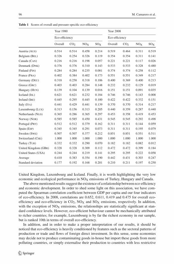
3.1 Some Comments on Eco-Efficiency
Table 1 displays several descriptive statistics for both overall and pressure-specific scoresof eco-efficiency in the years 1980 and 2008. First of all, the average of the eco-efficiencyindicators shows an upward trend over the sample period in all the definitions, except for NOX
emissions; furthermore, the highest average eco-efficiency scores at specific air pollutantlevel correspond to CO2 emissions. This seems quite reasonable if we bear in mind that thispollutant is the main contributor to global warming and that environmental regulations aimedat reducing carbon dioxide emissions have been in force the longest and in most cases arethe most restrictive.11
Secondly, Switzerland is the only economy that remains on the eco-efficient frontierthroughout the entire period studied. In other words, Switzerland is always the most eco-efficient country in the sample. Where overall eco-efficiency is concerned, the second bestperforming country in 2008 was Sweden, followed by Iceland, France, Norway and Denmark,that is, mostly Scandinavian countries. Conversely, Southern European economies such asPortugal, Spain and Greece, in addition to Hungary, Turkey, Canada and the United States,record the worst eco-efficiency scores. It is also interesting to highlight that overall eco-efficiency in countries such as Portugal, Spain, Greece and Turkey is lower in 2008 thanin 1980.12 In contrast, the largest improvements correspond to Sweden, Denmark, France,
11 Our scores of overall eco-efficiency are in fact largely determined by eco-efficiency in CO2 emissions, asthe proportional reduction in all three emissions is constrained in most countries by these emissions. In moretechnical words, due to greater effort being made to reduce CO2 emissions, restrictions on this pollutant inprogram (3) have more binding power.12 Kortelainen (2008) obtains the same result for Spain and Greece as regards the evolution of environmentalperformance between 1990 and 2003.
123
96 M. Camarero et al.
Table 1 Scores of overall and pressure-specific eco-efficiency
Year 1980 Year 2008
Eco-efficiency Eco-efficiency
Overall CO2 NOX SOX Overall CO2 NOX SOX
Austria (Aus) 0.514 0.514 0.458 0.214 0.519 0.464 0.311 0.519
Belgium (Bel) 0.326 0.254 0.326 0.119 0.354 0.354 0.311 0.141
Canada (Can) 0.216 0.216 0.198 0.057 0.221 0.221 0.117 0.026
Denmark (Dnk) 0.376 0.376 0.310 0.143 0.533 0.533 0.328 0.480
Finland (Fin) 0.284 0.284 0.235 0.081 0.374 0.374 0.258 0.112
France (Fra) 0.402 0.384 0.402 0.173 0.551 0.551 0.349 0.217
Germany (Deu) 0.318 0.258 0.318 0.106 0.400 0.369 0.400 0.213
Greece (Grc) 0.403 0.403 0.284 0.148 0.232 0.232 0.129 0.019
Hungary (Hun) 0.139 0.104 0.139 0.016 0.151 0.151 0.091 0.035
Iceland (Isl) 0.621 0.621 0.232 0.184 0.746 0.746 0.143 0.008
Ireland (Ire) 0.445 0.295 0.445 0.100 0.422 0.422 0.332 0.151
Italy (Ita) 0.441 0.429 0.441 0.139 0.370 0.370 0.314 0.217
Luxembourg (Lux) 0.313 0.156 0.313 0.205 0.440 0.359 0.287 0.440
Netherlands (Nld) 0.365 0.286 0.365 0.297 0.453 0.358 0.419 0.453
Norway (Nor) 0.585 0.585 0.450 0.431 0.545 0.545 0.292 0.498
Portugal (Prt) 0.512 0.512 0.379 0.162 0.311 0.311 0.144 0.059
Spain (Esp) 0.345 0.345 0.291 0.073 0.311 0.311 0.195 0.079
Sweden (Swe) 0.507 0.507 0.377 0.212 0.851 0.851 0.551 0.511
Switzerland (Che) 1.000 1.000 1.000 1.000 1.000 1.000 1.000 1.000
Turkey (Tur) 0.332 0.332 0.290 0.070 0.182 0.182 0.082 0.012
United Kingdom (GBr) 0.328 0.328 0.309 0.112 0.472 0.472 0.399 0.184
United States (USA) 0.244 0.244 0.219 0.141 0.295 0.295 0.222 0.058
Average 0.410 0.383 0.354 0.190 0.442 0.431 0.303 0.247
Standard deviation 0.177 0.192 0.168 0.201 0.210 0.211 0.197 0.250
United Kingdom, Luxembourg and Iceland. Finally, it is worth highlighting the very loweconomic and ecological performance in NOX emissions of Turkey, Hungary and Canada.
The above mentioned results suggest the existence of a relationship between eco-efficiencyand economic development. In order to shed some light on this association, we have com-puted the Spearman correlation coefficient between GDP per capita and our four indicatorsof eco-efficiency. In 2008, correlations are 0.652, 0.611, 0.419 and 0.475 for overall eco-efficiency and eco-efficiency in CO2, NOX and SOX emissions, respectively. In addition,with the exception of NOX emissions, the relationships are statistically significant at stan-dard confidence levels. However, eco-efficient behaviour cannot be mechanically attributedto richer countries; for example, Luxembourg is by far the richest economy in our sample,but is ranked 10th in terms of overall eco-efficiency.
In addition, and in order to make a proper interpretation of our results, it should benoticed that eco-efficiency is heavily conditioned by features such as the sectoral patterns ofproduction or trade and flows of foreign direct investment. In this sense, some economiesmay decide not to produce contaminating goods in-house but import these goods from morepolluting countries, or simply externalise their production to countries with less restrictive
123

Eco-Efficiency and Convergence in OECD Countries 97
Table 2 Convergence club classification
Overall eco-efficiency Eco-efficiencyin CO2 emissions
Eco-efficiencyin NOX emissions
Eco-efficiencyin SOX emissions
Club 1 Club 1 Club 1 Divergence
[Isl, Che, Swe] [Isl, Che, Swe] [Che, Swe]
log t t-stat log t t-stat log t t-stat log t t-stat
0.002 0.030 0.002 0.030 0.079 1.313 −0.366 −5.76∗∗Club 2 Club 2 Club 2 Club 1 (excluding
Dnk)[Aus, Dnk, Fra,
Deu, Ire, Lux,Nld, Nor, GBr]
[Aus, Dnk, Fra,Deu, Ire, Lux,Nor, GBr]
[Aus, Fra, Deu,Nld, GBr]
[Aus, Deu, Lux,Nld, Nor, Che,Swe]
log t t-stat log t t-stat log t t-stat log t t -stat
0.012 0.108 0.254 2.603 0.440 2.174 0.173 1.751
Club 3 Club 3 Club 3 Club 2 (excludingDnk)
[Bel, Fin, Ita, Prt,Esp, USA]
[Bel, Fin, Ita, Nld,Prt, Esp, USA]
[Bel, Dnk, Fin, Ire,Ita, Lux, Nor,USA]
[Fin, Fra, Ire, Ita,GBr]
log t t-stat log t t-stat log t t-stat log t t-stat
0.166 9.048 0.121 2.526 0.081 1.126 0.087 0.544
Club 4 Club 4 Club 4 Club 3 (excludingDnk)
[Can, Grc] [Can, Grc, Hun, Tur] [Can, Isl, Esp, Prt,Grc, Tur, Hun]
[Can, Hun, Prt,USA]
log t t-stat log t t-stat log t t-stat log t t-stat
0.404 12.04 0.315 5.744 0.331 1.162 0.219 2.790
Club 5 Non converging
[Hun, Tur] [Bel, Grc, Isl, Esp,Tur, Dnk]
log t t-stat log t t-stat
0.471 3.84 −2.285 −29.526∗∗
The clubs reported in this table have been obtained from the application of the algorithm proposed by Phillipsand Sul (2007). ‘log t’ stands for the parameter γ in Eq. (15), which is twice the speed of convergence, denotedas α, of this club towards the average; ‘t-stat’ is the convergence test statistic, distributed as a simple one-sidedt test (i.e. the critical value is −1.65). ** denote rejection
environmental regulations while retaining the ownership of the production. Nonetheless,an in-depth analysis of the factors behind differences in eco-efficiency among countries isbeyond the scope of this research.
3.2 Is there eco-efficiency convergence among OECD countries?
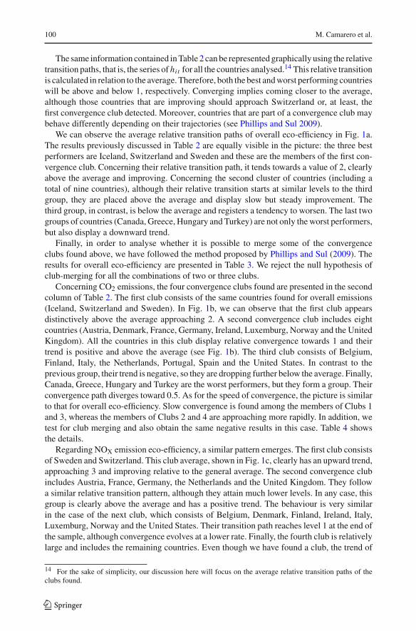
In this section we test for the existence of eco-efficiency convergence clubs using the indica-tors computed in Sect. 3.1 and the Phillips and Sul (2007) convergence algorithm described inSect. 3. The results for overall eco-efficiency emissions as well as for specific eco-efficiencyin CO2, NOX and SOX emissions are presented in Table 2 and Fig. 1.
123

98 M. Camarero et al.
0
0.5
1
1.5
2
CLUB 1 CLUB 2 CLUB 3 CLUB 4 CLUB 5
0
0.5
1
1.5
2
CLUB 1 CLUB 2 CLUB 3 CLUB 4
a
b
Fig. 1 Relative transition paths. Averages for the convergence clubs obtained in the Phillips and Sul (2007)analysis. a Overall eco-efficiency. b Eco-efficiency in CO2 emissions. c Eco-efficiency in NOx emissions.d Eco-efficiency in SOx emissions
Concerning overall eco-efficiency, the first column of Table 2 presents the five convergenceclubs obtained. We should take into account that the variable of interest is bounded betweenzero and one, where one denotes the most eco-efficient country, which was Switzerland inall cases. We proceed as follows: we find a first convergence club (Club 1) that consists ofIceland, Sweden and Switzerland. The other nineteen countries do not form a complementaryclub,13 so we look for a new and smaller convergence club (Club 2) which in this case containsnine countries (Austria, Denmark, France, Germany, Ireland, Luxemburg, the Netherlands,Norway and the United Kingdom). The next club (Club 3) consists of Belgium, Finland,Italy, Portugal, Spain and the United States, whereas Club 4 includes Canada and Greece.
13 The statistic was −28.527 (log t equal to −0.862), so we reject convergence for the group of countries.
123

Eco-Efficiency and Convergence in OECD Countries 99
0
0.5
1
1.5
2
2.5
3
CLUB 1 CLUB 2 CLUB 3 CLUB 4
0
0.5
1
1.5
2
2.5
CLUB 1 CLUB 2 CLUB 3
c
d
Fig. 1 continued
Finally, Club 5 has also two members: Hungary and Turkey. We should note that all countriesanalysed are classified in one of the five convergence clubs.
It is also worth mentioning that the speed of convergence is relatively slow for all theemissions considered in Table 2. This information can be gathered from the parameter pre-sented under the heading ‘log t’. This parameter is γ which is twice the value of α, the speedof convergence towards the average, and α ≥ 0 in the case of convergence. Regarding overalleco-efficiency, the first group, the best performers, records a value of α = 0.001. Convergenceis faster among other groups, implying that they are approaching one another more rapidlyin relative terms. We should bear in mind that the absolute best performer, Switzerland, isincluded in the first group.
123
100 M. Camarero et al.
The same information contained in Table 2 can be represented graphically using the relativetransition paths, that is, the series of hit for all the countries analysed.14 This relative transitionis calculated in relation to the average. Therefore, both the best and worst performing countrieswill be above and below 1, respectively. Converging implies coming closer to the average,although those countries that are improving should approach Switzerland or, at least, thefirst convergence club detected. Moreover, countries that are part of a convergence club maybehave differently depending on their trajectories (see Phillips and Sul 2009).
We can observe the average relative transition paths of overall eco-efficiency in Fig. 1a.The results previously discussed in Table 2 are equally visible in the picture: the three bestperformers are Iceland, Switzerland and Sweden and these are the members of the first con-vergence club. Concerning their relative transition path, it tends towards a value of 2, clearlyabove the average and improving. Concerning the second cluster of countries (including atotal of nine countries), although their relative transition starts at similar levels to the thirdgroup, they are placed above the average and display slow but steady improvement. Thethird group, in contrast, is below the average and registers a tendency to worsen. The last twogroups of countries (Canada, Greece, Hungary and Turkey) are not only the worst performers,but also display a downward trend.
Finally, in order to analyse whether it is possible to merge some of the convergenceclubs found above, we have followed the method proposed by Phillips and Sul (2009). Theresults for overall eco-efficiency are presented in Table 3. We reject the null hypothesis ofclub-merging for all the combinations of two or three clubs.
Concerning CO2 emissions, the four convergence clubs found are presented in the secondcolumn of Table 2. The first club consists of the same countries found for overall emissions(Iceland, Switzerland and Sweden). In Fig. 1b, we can observe that the first club appearsdistinctively above the average approaching 2. A second convergence club includes eightcountries (Austria, Denmark, France, Germany, Ireland, Luxemburg, Norway and the UnitedKingdom). All the countries in this club display relative convergence towards 1 and theirtrend is positive and above the average (see Fig. 1b). The third club consists of Belgium,Finland, Italy, the Netherlands, Portugal, Spain and the United States. In contrast to theprevious group, their trend is negative, so they are dropping further below the average. Finally,Canada, Greece, Hungary and Turkey are the worst performers, but they form a group. Theirconvergence path diverges toward 0.5. As for the speed of convergence, the picture is similarto that for overall eco-efficiency. Slow convergence is found among the members of Clubs 1and 3, whereas the members of Clubs 2 and 4 are approaching more rapidly. In addition, wetest for club merging and also obtain the same negative results in this case. Table 4 showsthe details.
Regarding NOX emission eco-efficiency, a similar pattern emerges. The first club consistsof Sweden and Switzerland. This club average, shown in Fig. 1c, clearly has an upward trend,approaching 3 and improving relative to the general average. The second convergence clubincludes Austria, France, Germany, the Netherlands and the United Kingdom. They followa similar relative transition pattern, although they attain much lower levels. In any case, thisgroup is clearly above the average and has a positive trend. The behaviour is very similarin the case of the next club, which consists of Belgium, Denmark, Finland, Ireland, Italy,Luxemburg, Norway and the United States. Their transition path reaches level 1 at the end ofthe sample, although convergence evolves at a lower rate. Finally, the fourth club is relativelylarge and includes the remaining countries. Even though we have found a club, the trend of
14 For the sake of simplicity, our discussion here will focus on the average relative transition paths of theclubs found.
123
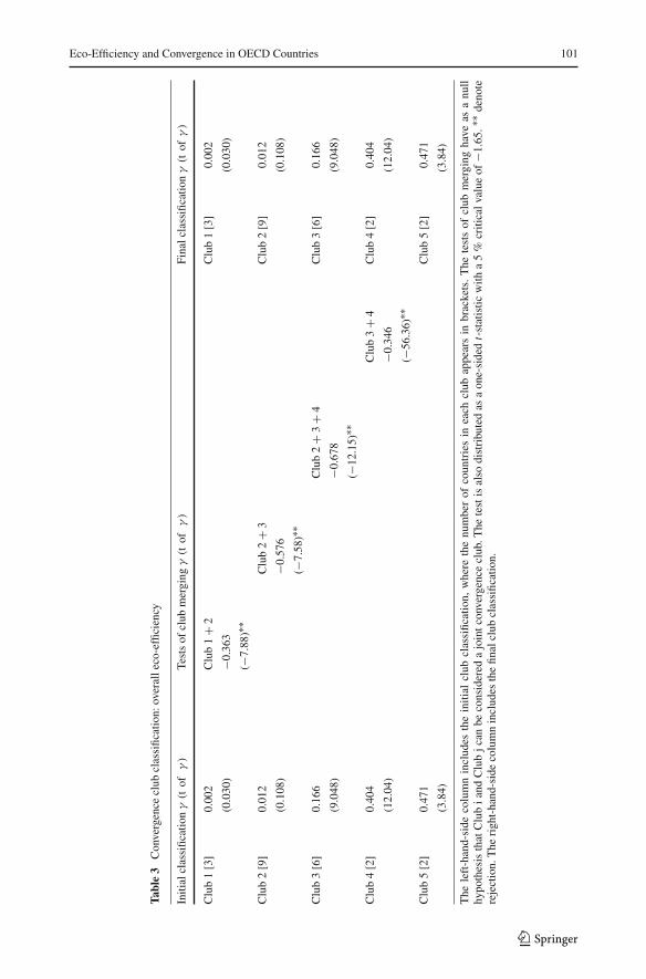
Eco-Efficiency and Convergence in OECD Countries 101
Tabl
e3
Con
verg
ence
club
clas
sific
atio
n:ov
eral
leco
-effi
cien
cy
Initi
alcl
assi
ficat
ion
γ(t
ofγ)
Test
sof
club
mer
ging
γ(t
ofγ)
Fina
lcla
ssifi
catio
nγ
(tof
γ)
Clu
b1
[3]
0.00
2C
lub
1+
2C
lub
1[3
]0.
002
(0.0
30)
−0.3
63(0
.030
)
(−7.
88)∗∗
Clu
b2
[9]
0.01
2C
lub
2+
3C
lub
2[9
]0.
012
(0.1
08)
−0.5
76(0
.108
)
(−7.
58)∗∗
Clu
b3
[6]
0.16
6C
lub
2+
3+
4C
lub
3[6
]0.
166
(9.0
48)
−0.6
78(9
.048
)
(−12
.15)
∗∗C
lub
4[2
]0.
404
Clu
b3
+4
Clu
b4
[2]
0.40
4
(12.
04)
−0.3
46(1
2.04
)
(−56
.36)
∗∗C
lub
5[2
]0.
471
Clu
b5
[2]
0.47
1
(3.8
4)(3
.84)
The
left
-han
d-si
deco
lum
nin
clud
esth
ein
itial
club
clas
sific
atio
n,w
here
the
num
ber
ofco
untr
ies
inea
chcl
ubap
pear
sin
brac
kets
.T
hete
sts
ofcl
ubm
ergi
ngha
veas
anu
llhy
poth
esis
that
Clu
bia
ndC
lub
jcan
beco
nsid
ered
ajo
intc
onve
rgen
cecl
ub.T
hete
stis
also
dist
ribu
ted
asa
one-
side
dt-
stat
istic
with
a5
%cr
itica
lval
ueof
−1.6
5.∗∗
deno
tere
ject
ion.
The
righ
t-ha
nd-s
ide
colu
mn
incl
udes
the
final
club
clas
sific
atio
n.
123

102 M. Camarero et al.
Table 4 Convergence club classification: eco-efficiency in CO2 emissions
Initial classification γ (t of γ ) Tests of club merging γ (t of γ ) Final classification γ (t of γ )
Club 1 [3] 0.002 Club 1 + 2 Club 1 [3] 0.002
(0.030) −0.21 (0.030)
(−14.13)∗∗Club 2 [8] 0.254 Club 2 + 3 Club 2 [8] 0.254
(2.603) −0.369 (2.603)
(−7.157)∗∗Club 3 [7] 0.121 Club 2 + 3 + 4 Club 3 [7] 0.121
(2.526) −0.507 (2.526)
(−11.78)∗∗Club 4 [4] 0.315 Club 4 [4] 0.315
(5.744) (5.744)
The left-hand-side column includes the initial club classification, where the number of countries in each clubappears in brackets. The tests of club merging have as a null hypothesis that Club i and Club j can be considereda joint convergence club. The test is also distributed as a one-sided t statistic with a 5 % critical value of −1.65.∗∗ denote rejection. The right-hand-side column includes the final club classification
Table 5 Convergence club classification: eco-efficiency in NOX emissions
Initial classification γ (t of γ ) Tests of club merging γ (t of γ ) Final classification γ (t of γ )
Club 1 [2] 0.079 Club 1 + 2 Club 1 [2] 0.079
(1.313) −5.109 (1.313)
(−10.495)∗∗Club 2 [5] 0.404 Club 2 + 3 Club 2 [5] 0.404
(2.174) −0.338 (2.174)
(−6.291)∗∗Club 3 [8] 0.081 Club 3 [8] 0.081
(1.126) (1.126)
Club 4 [7] 0.331 Club 4 [7] 0.331
(1.162) (1.162)
The left-hand-side column includes the initial club classification, where the number of countries in each clubappears in brackets. The tests of club merging have as a null hypothesis that Club i and Club j can be considereda joint convergence club. The test is also distributed as a one-sided t statistic with a 5 % critical value of −1.65.∗∗ denote rejection. The right-hand-side column includes the final club classification.
their transition path is clearly negative and attains such low levels that we may consider themalmost a diverging group. In Table 5 we present the club-merging results for NOX emissions.Inter-group convergence is again rejected for all the combinations analysed. As for the speedof convergence, the fastest is found in Club 2 (0.22) and the slowest again in Club 1 (0.04).
Finally, in the case of SOX emissions, we have found just one convergence club, whichincludes the majority of the countries. The only exceptions are Iceland, Greece and Por-tugal. However, although the algorithm has detected a convergence club, we should becautious: log t is negative (−0.366) and the t-statistic is −5.76, so convergence shouldbe rejected. Looking closely at the output obtained, the core group is very large: Switzer-land, the Netherlands, Sweden, Germany, France, Italy, the United States, Finland, Belgium,
123
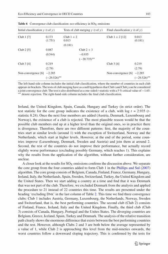
Eco-Efficiency and Convergence in OECD Countries 103
Table 6 Convergence club classification: eco-efficiency in SOX emissions
Initial classification γ (t of γ ) Tests of club merging γ (t of γ ) Final classification γ (t of γ )
Club 1 [7] 0.173 Club 1 + 2 Club 1 + 2 [12] 0.013(1.751) 0.013 (0.181)
(0.181)
Club 2 [5] 0.087 Club 2 + 3
(0.544) −0.935
(−20.735)∗∗Club 3 [4] 0.219 Club 3 [4] 0.219
(2.79) (2.79)
Non-convergence [6] −2.285 Non-convergence [6] −2.285
(−29.526)∗∗ (−29.526)∗∗
The left-hand-side column includes the initial club classification, where the number of countries in each clubappears in brackets. The tests of club merging have as a null hypothesis that Club i and Club j can be considereda joint convergence club. The test is also distributed as a one-sided t-statistic with a 5 % critical value of −1.65.∗∗ denote rejection. The right-hand-side column includes the final club classification.
Ireland, the United Kingdom, Spain, Canada, Hungary and Turkey (in strict order). Thetest statistic for the core group indicates the existence of a club, with log t = 2.935 (t-statistic 8.24). Once the next four members are added (Austria, Denmark, Luxembourg andNorway), the existence of a club is rejected. The most plausible reason would be that thepossible club members end up at a higher level than the original ones, so in practice thereis divergence. Therefore, there are two different patterns: first, the majority of the coun-tries start at similar levels (around 1) with the exception of Switzerland, Norway and theNetherlands, which start at higher levels. However, at the end of the period, some coun-tries improve (Luxembourg, Denmark, Sweden and Austria) and join them at around 2.Second, the rest of the countries do not improve their performance, but actually recordslightly worse performance (excluding possibly Germany, which reaches 1). This explainswhy the results from the application of the algorithm, without further consideration, areunclear.
A closer look at the results for SOX emissions confirms the discussion above. We separatethe core group from the four countries added to form Club 1 in the Phillips and Sul (2007)algorithm. The core group consists of Belgium, Canada, Finland, France, Germany, Hungary,Ireland, Italy, the Netherlands, Spain, Sweden, Switzerland, Turkey, the United Kingdom andthe United States. Then we start adding a country at a time and find that it was Denmarkthat was not part of the club. Therefore, we excluded Denmark from the analysis and appliedthe procedure to 21 instead of 22 countries this time. The results are presented under theheading ‘excluding Dnk’ in the last column of Table 2. This time we find three convergenceclubs: Club 1 includes Austria, Germany, Luxembourg, the Netherlands, Norway, Swedenand Switzerland, that is, the best performing countries. The second club (Club 2) consistsof Finland, France, Ireland, Italy and the United Kingdom. Finally, the third club (Club3) consists of Canada, Hungary, Portugal and the Unites States. The diverging countries areBelgium, Greece, Iceland, Spain, Turkey and Denmark. The analysis of the relative transitionpath clearly shows the enormous difference that exists between the best performing countriesand the rest. However, although Clubs 2 and 3 are both below the average represented bya value of 1, while Club 2 is approaching this level from the mid-nineties onwards, theworst countries follow a downward sloping trajectory. This is confirmed by the tests for
123
104 M. Camarero et al.
club-merging: the hypothesis is accepted for the case of Clubs 1 and 2 (see Table 6). Theseclubs exhibit the lowest values for speed of convergence. The merger between Clubs 1 and2 results in even slower convergence, whereas for Club 3 α = 0.110.
4 Summary and Concluding Remarks
The simplicity of the concept of economic and ecological efficiency and its inbuilt advantageof considering economics and ecology jointly has received increasing attention in political,academic and business circles. In addition, the assessment of eco-efficiency can be consid-ered a new instrument to provide policymakers with sound information to support decisionsthat contribute to longer-term sustainable development. Accordingly, a burgeoning literaturehas emerged in the last fifteen years aimed at assessing eco-efficiency at firm, industry oreconomy-wide level.
Starting from the most common definition of eco-efficiency as a relationship betweeneconomic performance and ecological performance, our aim is to study the existence ofconvergence in eco-efficiency among developed economies. For this purpose, we use a sampleof 22 OECD countries with data for the period 1980–2008. Concerning the methodology, in afirst stage we apply the recent approach to eco-efficiency measurement by Picazo-Tadeo et al.(2011) to compute scores of overall eco-efficiency as well as eco-efficiency in the emission ofthree specific air pollutants, namely, carbon dioxide, nitrogen oxides and sulphur oxides. In asecond stage, we follow Phillips and Sul (2007) to test for the existence of convergence clubsin eco-efficiency. To the best of our knowledge, the study of convergence in eco-efficiency atspecific environmental pressure and macro level constitutes our main contribution to previousliterature in this field.
Our main findings are summarised as follows. First, we find an upward trend in all oureco-efficiency indicators, with the only exception of nitrogen oxide emissions. Greater eco-efficiency corresponds to carbon dioxide emissions, probably due to the more demandingregulations in developed economies regarding this air pollutant. Switzerland is always the bestperforming country, while other economies that perform well are Sweden, Iceland, Norwayand Denmark. In contrast, the worst-performing economies are mostly Southern Europeancountries such as Portugal, Spain and Greece, in addition to Hungary, Turkey, Canada and theUnited States. A positive and statistically significant relationship between income per capitaand economic-ecological performance is also found. In addition, eco-efficiency is greatlyinfluenced by features such as the composition of a country’s economic activity and flowsof international trade and direct foreign investment. However, an analysis of these aspects isbeyond the scope of this paper.
Concerning the analysis of convergence, we find that the most eco-efficient countries tendto form convergence clubs by themselves, whereas the worst performers also tend to formclubs of convergence. Where overall eco-efficiency is concerned, five convergence clubsare found. While Iceland, Sweden and Switzerland form the first club of best performers,Hungary and Turkey form the fifth and last convergence club. Similar patterns are foundfor eco-efficiency in carbon dioxide and nitrogen oxide emissions, whereas in the case ofsulphur emissions we find three convergence clubs including the majority of the countries inthe sample.
The main policy implication of our results is that more stringent regulations on air pol-luting emissions are required in developed economies, particularly in countries displayinglower eco-efficiency levels. Furthermore, while the environmental regulations and inter-governmental agreements put into practice to date have mainly focused on carbon dioxide
123

Eco-Efficiency and Convergence in OECD Countries 105
emissions, future regulations and accords should pay close attention to reducing nitrogenand sulphur oxide emissions, for which developed countries record lower eco-efficiencyscores.
Finally, we would like to highlight that our research analyses convergence in eco-efficiencyat country and environmental pressure level, but further work is required in a topic of suchinterest to society and with great potential to help policymakers to design better environ-mental policies. In this sense, incorporating appropriate sectoral disaggregation of economicactivity in the assessment of eco-efficiency or relating eco-efficiency scores to foreign directinvestment flows, particularly those related to the vertical integration of production processes,are interesting avenues for further research. Accounting for more comprehensive and precisemeasures of pollution, the construction of composite indicators of environmental pressureswith non-linear structures, including some weight restrictions in line with recent work byZhou et al. (2010), developing more powerful methods to assess convergence or investigatinginto the determinants of eco-efficiency convergence are also interesting topics for future work.Broadening our knowledge in these directions is undoubtedly one of the greatest challengesfor future research in relation to sustainability.
Acknowledgments The authors thank the comments and suggestions from two anonymous referees. Thisresearch has been financed by the Spanish Ministry of Science and Technology (projects ECO2011-30260-C03-01 and ECO2012-32189). The authors also thank the financial aid received from the Generalitat Valenciana(program PROMETEO 2009/098).
References
Aldy JE (2006) Per capita carbon dioxide emissions: convergence or divergence? Environ Resour Econ33:533–555
Aldy JE (2007) Divergence in state-level per capita carbon dioxide emissions. Land Econ 83:353–369Allen R, Thanassoulis E (2004) Improving envelopment in data envelopment analysis. Eur J Oper Res 154:
363–379Barassi MR, Cole MA, Elliott RJR (2008) Stochastic divergence or convergence of per capita carbon dioxide
emissions: re-examining the evidence. Environ Resour Econ 40:121–137Barassi MR, Cole MA, Elliott RJR (2011) The stochastic convergence of CO2 emissions: a long memory
approach. Environ Resour Econ 49:367–385Camarero M, Picazo-Tadeo AJ, Tamarit C (2008) Is the environmental performance of industrialized countries
converging? A ‘SURE’ approach to testing for convergence. Ecol Econ 66:653–661Camarero M, Picazo-Tadeo AJ, Tamarit C (2013) Are the determinants of CO2 emissions converging among
OECD countries? Econ Lett 118:159–162Charnes A, Cooper WW, Rhodes E (1978) Measuring the efficiency of decision making units. Eur J Oper Res
2:429–444Cooper WW, Seiford LM, Tone K (2007) Data envelopment analysis. A comprehensive text with models,
applications, references and DEA-Solver software. Springer, New YorkEzcurra R (2007) Is there cross-country convergence in carbon dioxide emissions? Energ Policy 35:1363–1372Farrell MJ (1957) The measurement of productive efficiency. J R Stat Soc Ser A 120:253–281Figge F, Hahn T (2004) Sustainable value added-measuring corporate contributions to sustainability beyond
eco-efficiency. Ecol Econ 48:173–187Huppes G, Ishikawa M (2005) A framework for quantified eco-efficiency analysis. J Ind Ecol 9:25–41IPCC, Intergovernmental Panel on Climate Change (1990) Climate change: the IPCC scientific assessment.
In: Houghton JT, Jenkins GJ, Ephraums JJ (eds) The IPCC scientific assessment. Cambridge UniversityPress, Cambridge
IPCC, Intergovernmental Panel on Climate Change (2007) Climate change 2007: synthesis report. Switzerland,Geneva
Jobert T, Karanfil F, Tykhonenko A (2010) Convergence of per capita carbon dioxide emissions in the EU:legend or reality? Energy Econ 32:1364–1373
123
106 M. Camarero et al.
Koopmans T (1951) Analysis of production as an efficient combination of activities. In: Koopmans T (ed)Activity analysis of production and allocation. Wiley, New York
Kortelainen M (2008) Dynamic environmental performance analysis: a Malmquist index approach. Ecol Econ64:701–715
Kuosmanen T, Kortelainen M (2005) Measuring eco-efficiency of production with data envelopment analysis.J Ind Ecol 9:59–72
Lanne M, Liski M (2004) Trends and breaks in per-capita carbon dioxide emissions, 1870–2028. Energy J25:41–65
Lee C, Chang C (2008) New evidence on the convergence of per capita carbon dioxide emissions from panelseemingly unrelated regressions augmented Dickey-Fuller tests. Energy 33:1468–1475
Lee C, Chang C (2009) Stochastic convergence of per capita carbon dioxide emissions and multiple structuralbreaks in OECD countries. Econ Model 26:1375–1381
Nourry M (2009) Re-examining the empirical evidence for stochastic convergence of two air pollutants witha pair-wise approach. Environ Resour Econ 44:555–570
Organization for Economic Cooperation and Development, OECD (1998) Eco-efficiency. OECD, ParisOrdás Criado C, Grether JM (2011) Convergence in per capita CO2 emissions: a robust distributional approach.
Resour Energy Econ 33:637–665Panopoulou E, Pantelidis T (2009) Club convergence in carbon dioxide emissions. Environ Resour Econ
44:47–70Phillips PCB, Sul D (2007) Transition modeling and econometric convergence tests. Econometrica 75:
1771–1855Phillips PCB, Sul D (2009) Economic transition and growth. J Appl Econom 24:1153–1185Picazo-Tadeo AJ, Reig-Martínez E, Gómez-Limón JA (2011) Assessing farming eco-efficiency: a data envel-
opment analysis approach. J Environ Manag 92:1154–1164Porter ME, van der Linde C (1995) Toward a new conception of the environment-competitiveness relationship.
J Econ Perspect 9:97–118Romero-Ávila D (2008) Convergence in carbon dioxide emissions among industrialized countries revisited.
Energy Econ 30:2265–2282Schaltegger S (1996) Corporate environmental accounting. Wiley, ChichesterSchmidheiny S, Zorraquin FJL (1996) Financing change, the financial community, eco-efficiency and sustain-
able development. MIT Press, CambridgeTorgersen A, Førsund F, Kittelsen S (1996) Slack-adjusted efficiency measures and ranking of efficient units.
J Prod Anal 7:379–398United Nations (2009) Eco-efficiency indicators: measuring resource-use efficiency and the impact of eco-
nomic activities on the environment. Greening of Economic Growth Series, ST/ESCAP/2561WBCSD, World Business Council for Sustainable Development (2000) Eco-efficiency: creating more value
with less impact. WBSCD, GenevaWesterlund J, Basher S (2008) Testing for convergence in carbon dioxide emissions using a century of panel
data. Environ Resour Econ 40:109–120Wursthorn S, Poganietz WR, Schebek L (2011) Economic-environmental monitoring indicators for European
countries: a disaggregated sector-based approach for monitoring eco-efficiency. Ecol Econ 70:487–496Zhang B, Bi J, Fan Z, Yuan Z, Ge J (2008) Eco-efficiency analysis of industrial system in China: a data
envelopment analysis approach. Ecol Econ 68:306–316Zhou P, Ang BW, Poh KL (2008) A survey of data envelopment analysis in energy and environmental studies.
Eur J Oper Res 189:1–18Zhou P, Ang BW, Zhou DQ (2010) Weighting and aggregation in composite indicator construction: a multi-
plicative optimization approach. Soc Indic Res 96:169–181
123

Reproduced with permission of the copyright owner. Further reproduction prohibited withoutpermission.