econometria ii. curso 2009/2010 lab # 3 box-jenkins ... · econometria ii. curso 2009/2010 lab # 3...

2

ECONOMETRIA II. CURSO 2009/2010 LAB # 3 BOX-JENKINS’ METHODOLOGY

The Box Jenkins’ approach combines the moving average and the

autorregresive models. Although both models were already known, the contribution

of Box and Jenkins was in developing a systematic methodology for identifying and

estimating models that could incorporate both approaches.

There are three primary stages in building a Box-Jenkins time series model:

o Model identification

o Model Estimation o Model Validation

MODEL IDENTIFICATION: It consists to determine the adequate model from ARIMA family models. At

this step, the parameters of the ARIMA model,

ARIMA (p,d,q) x (P,D,Q)s

will be identified.

The first step in developing a Box-Jenkins model is to determine if the series

is stationary and if there is any significant seasonality that needs to be modelled. If

the time series is not stationary, Box-Jenkins proposed to find its stationary

transformation by differencing the time series:

Zt = (1-B)d (1-Bs ) D

3

where d is the number of regular differences and D corresponds to the Lumber of

seasonal differences. Generally, D = 0 ó 1 and 0 ≤ d+D ≤ 2.

This phase is founded on the study of the autocorrelation (acf) and partial

autocorrelation (pacf), and unit root tests (we will use the Augmented Dickey Fuller

test, ADF)

Once d and D are fixed, the acf and pacf are used to determined the orders

of the autorregresive process (p) and the moving average process (q). Next table

summarizes the features of the fac and the pacf for each type of model:

The type of stationary model Process ACF PACF

AR (p) Exponential, decaying to zero P spikes, rest are essentially

zero

MA (p) q spikes, rest are essentially

zero Exponential, decaying to zero

ARMA (p, q) Decay exponentially, starting

alter few lags

Decay exponentially, starting

alter few lags

In the Identification step, more than one model will be usually proposed (there

will be several tentative models that could be fitted to the time series). All these

models will be estimated (second step) and, finally, according to the third step

(Model Validation), we will apply some tests on the coefficients and the residuals

that allow us to choose the ‘best’ model.

MODEL ESTIMATION: Maximum likelihood estimation is generally the preferred technique to fit Box-

Jenkins models. However, Eviews has not implemented this technique and it uses

the method of least squares (LS).

MODEL VALIDATION: o The estimates of the coefficients should be significantly different of 0.

o The AR and MA parameters should satisfy stationary and invertibility

conditions.

o No multicolinearity

4

o The residuals should be white noise

o Akaike and Schwartz criteria

In this practice, we will use three univariate time series: ‘ventas’, ‘empleo’,

and ‘puros’.

1. Ventas ‘Ventas’ is a time series that corresponds to the annual sales of a particular

company. It is available annually (then, it has not seasonal component) and it has

51 observations (from 1949 to 1999).

We have the workfile where the variable of interest is ventas. First of all, we

verify if the time series is stationary or not. If it is not stationary, we transform it to

achieve stationarity.

First of all, we plot the time series:

Quik/Graph /ventas/Line Graph

500

600

700

800

900

1000

1100

1200

50 55 60 65 70 75 80 85 90 95

VENTAS

Evolución de las ventas

It is continuously increasing (not constant mean) and the logarithm

transformation is not needed.

We look at its correlogram

Quick/Series Statistics/Correlogram/ventas

5

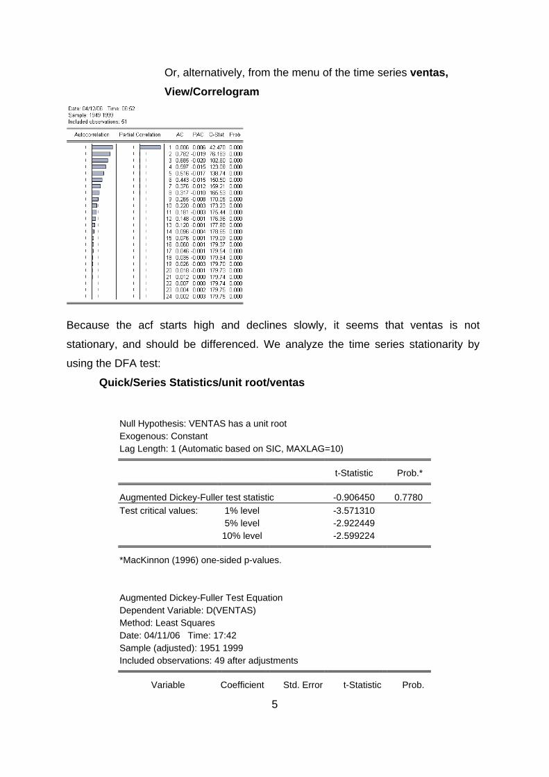
Or, alternatively, from the menu of the time series ventas, View/Correlogram

Because the acf starts high and declines slowly, it seems that ventas is not

stationary, and should be differenced. We analyze the time series stationarity by

using the DFA test:

Quick/Series Statistics/unit root/ventas

Null Hypothesis: VENTAS has a unit root Exogenous: Constant Lag Length: 1 (Automatic based on SIC, MAXLAG=10)

t-Statistic Prob.*

Augmented Dickey-Fuller test statistic -0.906450 0.7780 Test critical values: 1% level -3.571310

5% level -2.922449 10% level -2.599224

*MacKinnon (1996) one-sided p-values.

Augmented Dickey-Fuller Test Equation Dependent Variable: D(VENTAS) Method: Least Squares Date: 04/11/06 Time: 17:42 Sample (adjusted): 1951 1999 Included observations: 49 after adjustments

Variable Coefficient Std. Error t-Statistic Prob.

6

VENTAS(-1) -0.001026 0.001132 -0.906450 0.3694 D(VENTAS(-1)) 0.577317 0.111009 5.200645 0.0000

C 5.282546 1.831241 2.884682 0.0059

R-squared 0.454475 Mean dependent var 10.49688 Adjusted R-squared 0.430757 S.D. dependent var 1.402848 S.E. of regression 1.058424 Akaike info criterion 3.010708 Sum squared resid 51.53198 Schwarz criterion 3.126534 Log likelihood -70.76235 F-statistic 19.16125 Durbin-Watson stat 2.399094 Prob(F-statistic) 0.000001

According to the results the null hipótesis is not rejected. Then, ventas is not

stationary. First to remove the trend of ventas, we propose to fit a linear

deterministic trend:

ventas = c +β t + εt (1)

and estimate this model as:

Quick /estimate equation ventas c @trend+1

Dependent Variable: VENTAS Method: Least Squares Date: 04/09/06 Time: 19:17 Sample: 1949 1999 Included observations: 51


C 605.9019 1.299179 466.3730 0.0000 @TREND+1 10.39500 0.043483 239.0563 0.0000


7

-16

-12

-8

-4

0

4

8

12

50 55 60 65 70 75 80 85 90 95

VENTAS Residuals

We see that the residuals are not a White Boise process, then model (1) is

not a good model for ventas.

We take the first difference of ventas, Dventas =ventas-ventas(-1), and

transform the time series according to:

Zt =(1-B)ventas

The plot and the correlograms of the transformed time series, dventas, are:

7

8

9

10

11

12

13

14

15

50 55 60 65 70 75 80 85 90 95

D VENTAS

P rimera diferencia de la serie venta s

8

Both, the Plot and the acf indicate that dventas could be stationary. We

complete the analysis using the DFA test for dventas

D-F Aumentado test for Dventas

Null Hypothesis: DVENTAS has a unit root Exogenous: Constant Lag Length: 0 (Automatic based on SIC, MAXLAG=10)

t-Statistic Prob.*


5% level -2.922449 10% level -2.599224


Augmented Dickey-Fuller Test Equation Dependent Variable: D(DVENTAS) Method: Least Squares Date: 04/11/06 Time: 21:55 Sample (adjusted): 1951 1999 Included observations: 49 after adjustments


DVENTAS(-1) -0.381068 0.100878 -3.777505 0.0004

9

C 3.942637 1.078866 3.654428 0.0006

R-squared 0.232898 Mean dependent var -0.092714 Adjusted R-squared 0.216577 S.D. dependent var 1.193536 S.E. of regression 1.056413 Akaike info criterion 2.987596 Sum squared resid 52.45244 Schwarz criterion 3.064813 Log likelihood -71.19611 F-statistic 14.26955 Durbin-Watson stat 2.473364 Prob(F-statistic) 0.000445

The null hipótesis is rejected. Then the series dventas is sationary, and

Zt = (1-B) ventas o ventas ∼I (1)

Is the stationary transformation of ventas.

Next, we analyze the correlogram of dventas in order to determine the

tentative ARMA models. Two models are proposed: AR(2) and MA(3).

1.1) ARIMA(2,1,0) : (1-φ1B- φ2B2 ) (1-B) ventas = C+at

1.2) ARIMA(0,1,3) : (1-B) ventas = C+ (1+ θ1B+ θ2B2+ θ3B3)at

Estimation Both alternative models are estimated using Eviews:

Model 1.1: Quick/Estimate Equation/ LS d(ventas,1) c ar(1) ar(2) Model 1.2: Quick/Estimate Equation/ LS d(ventas,1) c ma(1) ma(2) ma(3) The results are:

Model1.1

Dependent Variable: DVENTAS Method: Least Squares Date: 04/09/06 Time: 19:10 Sample (adjusted): 1952 1999 Included observations: 48 after adjustments Convergence achieved after 3 iterations


C 10.11214 0.616994 16.38936 0.0000 AR(1) 0.368149 0.135783 2.711310 0.0095 AR(2) 0.388732 0.127968 3.037719 0.0040

R-squared 0.525916 Mean dependent var 10.45896 Adjusted R-squared 0.504846 S.D. dependent var 1.392085

10

S.E. of regression 0.979571 Akaike info criterion 2.857057 Sum squared resid 43.18014 Schwarz criterion 2.974007 Log likelihood -65.56936 F-statistic 24.95999 Durbin-Watson stat 1.991277 Prob(F-statistic) 0.000000

Inverted AR Roots .83 -.47

Model 1.2

Dependent Variable: DVENTAS Method: Least Squares Date: 04/09/06 Time: 19:02 Sample (adjusted): 1950 1999 Included observations: 50 after adjustments Convergence achieved after 13 iterations Backcast: 1946 1948


C 10.43083 0.392970 26.54353 0.0000 MA(1) 0.497157 0.101433 4.901323 0.0000 MA(2) 0.564666 0.097743 5.777057 0.0000 MA(3) 0.632436 0.086339 7.324991 0.0000


Inverted MA Roots .15-.88i .15+.88i -.79

Validation: In this step, we make the diagnostic of the two models, based on several tests. We

focus on the estimation results, the analysis of the residuals, and the Akaike and

Schwatz criteria to compare the models.

o Estimation Results The coefficients of the model should be significantly different of zero (the t-test).

Furthermore, the AR and MA coefficients should satisfy the stationary and

invertibility conditions of the model. Finally, in order to guarantee the stability of

the estimates, the correlation coefficients among the estimated parameters

11

should be close to zero (no multicollinearity). Then, in the MENU of the equation

(where we estimate the model)

View/Correlation Matrix

mode 1.1:

C AR(1) AR(2) C 0.380682 -0.005342 -0.015880

AR(1) -0.005342 0.018437 -0.011620 AR(2) -0.015880 -0.011620 0.016376

Low values for the model 1.2. too. No multicollinearity.

o Residuals analysis. Are the residuals white noise? We look the plot and the correlogram of the

residuals, and the Box-Pierce Q statistic. In the menu of the equation:

View/ Residual Tests/Correlogram-Q-Statistics Correlogram of the residuals (model 1)

The autocorrelation coefficients are not significantly different of 0. Furthermore,

according to the values of the Q statistic, the null hypothesis of joint dependence

among the residuals is rejected.

Plot the residuals: View/Actual, Fitted, residuals

12

-3

-2

-1

0

1

2

6

8

10

12

14

16

55 60 65 70 75 80 85 90 95

Residual Actual Fitted

It shows that there is not autocorrelation in the residuals (only the observation of

1962 is out of the confidence bands). Then, it seems that the residuals are White

noise.

The same analysis for the model 2 provides equivalent results.

o Criteria to compare the models The residual variance and the values of both, Akaike and Schwarz criteria, are

lower for the Model 1. Then Model 1 is the ‘optimal’ model for ventas.

2. Employment index The data are the employment indexo f a particular country. The time series is

seasonally adjusted. It is available quarterly from 1962:1 1993:4. It is called empleo. The procedure is similar to the previous one for the time series ventas. Then,

there are some stops that will not be repeated here

First, we plot the data: Quick/ Graph/ Graph Line/empleo

13

The time series is increasing during the first 20 years 20 and then there is a cyclical

components (the 10 last years). It seems to have constant variance but, in order to

analyze that point, we generate the logarithmic transformation of empleo

GENR Lempleo =LOG(empleo) And Plot it

Quick/ Graph/ Graph Line/ empleo

Grafico 1 a Gráfico 1b

80

85

90

95

100

105

110

115

1965 1970 1975 1980 1985 1990

EMPLEO

4.40

4.45

4.50

4.55

4.60

4.65

4.70

4.75

1965 1970 1975 1980 1985 1990

LEMPLEO

There is no difference between the two grapas, then we will consider the original

time series, empleo

Correlogram of empleo. In the menu of the variable empleo, View/Correlogram

14

The acf starts high and declines slowly, then it seems that empleo is not stationary,

and should be differenced. We analyze the time series stationarity by using the DFA

test:

Quick/ SERIES STATISTIC/ Unit root / empleo

DFA test empleo

Null Hypothesis: EMPLEO has a unit root Exogenous: Constant Lag Length: 1 (Automatic based on SIC, MAXLAG=12)

t-Statistic Prob.*


5% level -2.884477 10% level -2.579080


Augmented Dickey-Fuller Test Equation Dependent Variable: D(EMPLEO) Method: Least Squares Date: 04/19/08 Time: 21:29 Sample (adjusted): 1962Q3 1993Q4 Included observations: 126 after adjustments


EMPLEO(-1) -0.039278 0.017807 -2.205738 0.0293 D(EMPLEO(-1)) 0.478736 0.078727 6.080986 0.0000

C 3.982081 1.807249 2.203394 0.0294


15

El test DFA does not reject the null hyphotesis. Then, empleo should be

differentiated. We take the first differences of empleo, and show the Plot and the

correlogram of the transformation (dempleo) Genr DEMPLEO =D(EMPLEO,1) Quick/Graph/Line Graph/DEMPLEO

Quick/Series Statistic/Correlogram

-6

-4

-2

0

2

4

6

8

1965 1970 1975 1980 1985 1990

D(EMPLEO,1)

16

The graph and the correlogram (that decays exponentially) show that DEMPLEO.

The DFA test for DEMPLEO confirms this result.

DFA test DEMPLEO

Null Hypothesis: D(EMPLEO,1) has a unit root Exogenous: Constant Lag Length: 0 (Automatic based on SIC, MAXLAG=12)

t-Statistic Prob.*


5% level -2.884477 10% level -2.579080


Augmented Dickey-Fuller Test Equation Dependent Variable: D(EMPLEO,2) Method: Least Squares Date: 04/19/08 Time: 21:28 Sample (adjusted): 1962Q3 1993Q4 Included observations: 126 after adjustments


D(EMPLEO(-1),1) -0.537417 0.079598 -6.751657 0.0000 C 0.006063 0.131846 0.045988 0.9634


Then, EMPLEO has one regular unit root and, its stationary transformation is given

by

Zt =(1-B)EMPLEO o EMPLEO ∼I(1)

17

Next, we analyze the correlogram of DEMPLEO in order to determine the

tentative ARMA models. Three models are proposed: ARIMA (1,1,0), ARIMA(1;1,2) y

ARIMA(2,1,1). It seems that dempleo has zero men, then we do not include the

constant term in the estimation of the models

2.1. ARIMA(1,1,0) o (1- φ1 B)(1-B)EMPLEO = at

2.2. ARIMA(1,1,2) ) o (1- φ1 B )(1-B)EMPLEO= (1+ θ1B+θ2B2)at

2.3. ARIMA(2,1,1) ) o (1- φ1 B- φ2 B2) (1-B)EMPLEO= (1+ θ1B) at

Estimation In Eviews,

2.1. Quick/ Estimate Equation/ LS EMPLEO ar(1) 2.2. Quick/ Estimate Equation/ LS EMPLEO ar(1) ma(1) ma(2) 2.3. Quick/ Estimate Equation/ LS EMPLEO ar(1) ar(2) ma(1) Results: Model 2.1

Dependent Variable: D(EMPLEO,1) Method: Least Squares Date: 04/21/08 Time: 00:48 Sample (adjusted): 1962Q3 1993Q4 Included observations: 126 after adjustments Convergence achieved after 2 iterations


AR(1) 0.462622 0.079275 5.835666 0.0000

R-squared 0.214051 Mean dependent var 0.014150 Adjusted R-squared 0.214051 S.D. dependent var 1.662605 S.E. of regression 1.473962 Akaike info criterion 3.621689 Sum squared resid 271.5704 Schwarz criterion 3.644200 Log likelihood -227.1664 Durbin-Watson stat 2.029500

Inverted AR Roots .46

18

Model 2.2

Dependent Variable: D(EMPLEO,1) Method: Least Squares Date: 04/21/08 Time: 01:37 Sample (adjusted): 1962Q3 1993Q4 Included observations: 126 after adjustments Convergence achieved after 8 iterations Backcast: 1961Q3 1961Q4


AR(1) 0.515070 0.312357 1.648981 0.1017 MA(1) -0.070881 0.324334 -0.218544 0.8274 MA(2) 0.008407 0.170031 0.049446 0.9606


Inverted AR Roots .52 Inverted MA Roots .04+.08i .04-.08i

Model 2.3

Dependent Variable: D(EMPLEO,1) Method: Least Squares Date: 04/21/08 Time: 01:12 Sample (adjusted): 1962Q4 1993Q4 Included observations: 125 after adjustments Convergence achieved after 19 iterations Backcast: 1961Q4


AR(1) -0.459695 0.094065 -4.886990 0.0000 AR(2) 0.426099 0.082802 5.145983 0.0000 MA(1) 0.956981 0.046168 20.72805 0.0000


Inverted AR Roots .46 -.92 Inverted MA Roots -.96

19

Validation Model 2.1 and Model 2.3: all the coefficients are significantly different of 0. However,

in the Model 2.2., the MA parameters are not significantly different of 0. Then, model

2.2. is discarded. In the Model 2.1 and Model 2.3 the stationary and invertibility

conditions are satisfied. Additionally there is not multicollinearity in both models.

The residuals for model 2.1. and 2.3. are White noise. (see the correlograms of the

residuals, the plots, and the values of the Q-statistic). The residuals of both model,

2.1. and 2.3., have two aoutliers: 1987:01 and 1992:01.

Correlogram of the residuals (model 2.1)

20

Residuals graph (model 2.1)

-4

0

4

8

-8

-4

0

4

8

1965 1970 1975 1980 1985 1990



21

Residuals graph (model 2.3)

-4

0

4

8

-8

-4

0

4

8

1965 1970 1975 1980 1985 1990


The estándar error in Model 2.1 (1,4739) is lower than the corresponding to model

2.3 (1,4628). The value of Akaike is the same for both models (3,622).

3. Cigars sales

The tirad time series is a monthly time series from 1989:01 to 1996:12 that

represents the cigars sales of a particular company. It has clear trend and seasonal

pattern. It is called puros

Plot the time series: Quick/Graph/ puros/Line graph

200

300

400

500

600

700

800

1989 1990 1991 1992 1993 1994 1995 1996

PUROS

Ventas de puros de una empresa tabaquera

22

The level of puros decreases. It exhibits a clear trend (then its mean is not

constant over time ans the time series is not stationary) and a regular seasonal

pattern. Probably puros needs a regular and a seasonal differences in order to be

stationary. It is not clear if puros has constant variance (the vaiance is higher at the

beginning of the sample). We take logs, plot the log transformation, and analyze the

situation:

GENR Lpuros= log(puros) Quick/Graph/ Lpuros/Line graph

5.4

5.6

5.8

6.0

6.2

6.4

6.6

1989 1990 1991 1992 1993 1994 1995 1996

LPUROS

Evolución logaritmica de las ventas de puros

Lpuros is similar to puros then we decide to work with the original time

series.

Make the correlogram. In the menu of the variable puros, View/ Correlogram

23

The correlogram decays slowly in the regular lags (1,2,3,etc) and in the seasonal too

(12,24,36,etc). Then, the seasonal pattern of puros is clear. First, we take ine regular

difference, and plot the transformation, dpuros. Additionally, we make the

correlogram of dpuros Genr dpuros=D(puros,1) Quick/Graph/dpuros/Line graph Quick/series statistic/correlogram/dpuros

-250

-200

-150

-100

-50

0

50

100

150

1990 1991 1992 1993 1994 1995 1996

DPUROS

24

The regular difference, d(puros,1), does not remove the non-satitonarity in the

seasonal part( the acf for the seasonal lags decays slowly and takes very high

values). Then, we should differentiate the time series again, and take a seasonal

difference for dpuros. The new transformation, denoted by dd12puros, is plotted

and we analyze its correlogram:

Genr dd12puros=d(puros,1,12) Quick/Graph/Line Graph/dd12puros Quick/series statistic/correlogram/dd12puros

-150

-100

-50

0

50

100

150

1990 1991 1992 1993 1994 1995 1996

DD12PUROS

25

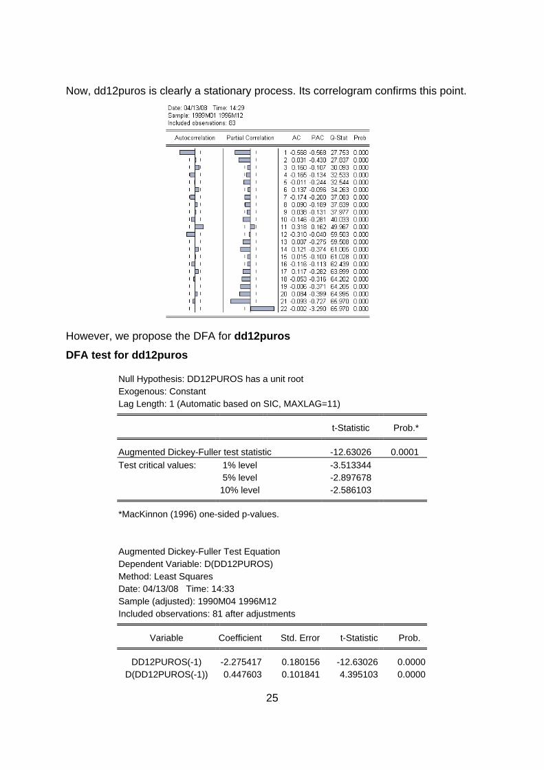
Now, dd12puros is clearly a stationary process. Its correlogram confirms this point.

However, we propose the DFA for dd12puros DFA test for dd12puros

Null Hypothesis: DD12PUROS has a unit root Exogenous: Constant Lag Length: 1 (Automatic based on SIC, MAXLAG=11)

t-Statistic Prob.*


5% level -2.897678 10% level -2.586103


Augmented Dickey-Fuller Test Equation Dependent Variable: D(DD12PUROS) Method: Least Squares Date: 04/13/08 Time: 14:33 Sample (adjusted): 1990M04 1996M12 Included observations: 81 after adjustments


DD12PUROS(-1) -2.275417 0.180156 -12.63026 0.0000 D(DD12PUROS(-1)) 0.447603 0.101841 4.395103 0.0000

26

C -0.630273 4.413679 -0.142800 0.8868


The results of the DFA confirms that dd12puros is stationary (t-statistic, -12.630 is

higher than the critical values of the DFA distribution). Then, the stationary

transformation of puros is:

Zt =(1-B) (1-B12)puros Now, we should decide the values of p,q, P, and Q for the general ARIMA model

(multiplicative ARIMA model)

ARMA (p,q) Χ ARMA(P,Q)S

According to the correlogram of dd12puros, the regular part could be model by a

MA(1) or AR(2) process, while the seasonal part is clearly a MA(1)12 . Then, the two

alternative models that we will consider are:

3.1. ARIMA(0,1,1)×(0,1,1)12 o (1-B)(1-B12)puros= (1+ θ1B)(1+θ12B12)at

3.2. ARIMA(2,1,0)×(0,1,1)12 ,, (1- φ1B-φ2B2) (1-B)(1-B12) puros= (1+θ12B12)at Estimation (model 3.1)

Dependent Variable: DD12PUROS Method: Least Squares Date: 04/13/08 Time: 18:09 Sample (adjusted): 1990M02 1996M12 Included observations: 83 after adjustments Convergence achieved after 14 iterations Backcast: 1987M12 1988M12


MA(1) -0.677779 0.066918 -10.12847 0.0000 SMA(12) -0.867044 0.034549 -25.09612 0.0000

R-squared 0.662434 Mean dependent var -0.481928 Adjusted R-squared 0.658267 S.D. dependent var 52.83531 S.E. of regression 30.88643 Akaike info criterion 9.722312

27

Sum squared resid 77271.69 Schwarz criterion 9.780597 Log likelihood -401.4760 Durbin-Watson stat 2.546859

Inverted MA Roots .99 .86-.49i .86+.49i .68 .49-.86i .49+.86i .00+.99i -.00-.99i -.49-.86i -.49+.86i -.86+.49i -.86-.49i -.99

Residual Graph (model 3.1)

-80

-40

0

40

80

1990 1991 1992 1993 1994 1995 1996

DD12PUROS Residuals


28

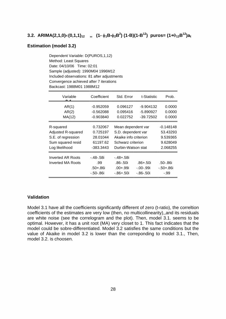
3.2. ARIMA(2,1,0)×(0,1,1)12 ,, (1- φ1B-φ2B2) (1-B)(1-B12) puros= (1+θ12B12)at Estimation (model 3.2)

Dependent Variable: D(PUROS,1,12) Method: Least Squares Date: 04/10/06 Time: 02:01 Sample (adjusted): 1990M04 1996M12 Included observations: 81 after adjustments Convergence achieved after 7 iterations Backcast: 1988M01 1988M12

Variable Coefficient Std. Error t-Statistic Prob. 3 1

AR(1) -0.952059 0.096127 -9.904132 0.0000 AR(2) -0.562088 0.095416 -5.890927 0.0000

MA(12) -0.903840 0.022752 -39.72502 0.0000

R-squared 0.732067 Mean dependent var -0.148148 Adjusted R-squared 0.725197 S.D. dependent var 53.43293 S.E. of regression 28.01044 Akaike info criterion 9.539365 Sum squared resid 61197.62 Schwarz criterion 9.628049 Log likelihood -383.3443 Durbin-Watson stat 2.068255

Inverted AR Roots -.48-.58i -.48+.58i Inverted MA Roots .99 .86-.50i .86+.50i .50-.86i

.50+.86i .00+.99i -.00-.99i -.50+.86i -.50-.86i -.86+.50i -.86-.50i -.99

Validation Model 3.1 have all the coefficients significantly different of zero (t-ratio), the correltion coefficients of the estimates are very low (then, no multicollinearity),,and its residuals are white noise (see the correlogram and the plot). Then, model 3.1. seems to be optimal. However, it has a unit root (MA) very closet to 1. This fact indicates that the model could be sobre-differentiated. Model 3.2 satisfies the same conditions but the value of Akaike in model 3.2 is lower than the correponding to model 3.1., Then, model 3.2. is choosen.

econometria ii. curso 2009/2010 lab # 3 box-jenkins ... · econometria ii. curso 2009/2010 lab # 3...

Documents