Economic and Social Networks: Lecture 6

Adam Szeidl

November 2, 2016

Outline for today

1 Input-output networks and aggregate fluctuations

2 Interfirm relationships: evidence

1 / 24

1. Firm networks

• Classic diversification argument: micro shocks cannot haveaggregate effects.

• Independent sectoral shocks’ impact proportional to√n, negligible at

high disaggregation.

• Acemoglu, Carvalho, Ozdaglar, Tahbaz-Salehi (2012): argumentmay fail with intersectoral linkages.

• Example: in 2008 Ford chief requested govt support for GM andChrysler.

• Because Ford worried about competitors’ default seriously hurtingcommon suppliers.

• How does input-output network structure shape impact of microshocks?

2 / 24

Example networks

NETWORK ORIGINS OF AGGREGATE FLUCTUATIONS 1979

(a) (b)

FIGURE 1.—The network representations of two symmetric economies. (a) An economy inwhich no sector relies on other sectors for production. (b) An economy in which each sectorrelies equally on all other sectors.

all others. In this case, as n increases, sectoral shocks do not average out: evenwhen n is large, shocks to sector 1 propagate strongly to the rest of the econ-omy, generating significant aggregate fluctuations.

Even though the “star network” in Figure 2 illustrates that, in the presence ofinterconnections, sectoral shocks may not average out, it is also to some extentan extreme example. A key question, therefore, is whether the effects of mi-croeconomic shocks can be ignored in economies with more realistic patternsof interconnections. The answer naturally depends on whether the intersec-toral network structures of actual economies resemble the economies in Fig-ure 1 or the star network structure in Figure 2. Figure 3 gives a first glimpse ofthe answer by depicting the input–output linkages between 474 U.S. industriesin 1997. It suggests that even though the pattern of sectoral interconnectionsis not represented by a star network, it is also significantly different from thenetworks depicted in Figure 1. In fact, as our analysis in Section 4 shows, inmany ways the structure of the intersectoral input–output relations of the U.S.economy resembles that of Figure 2, as a small number of sectors play a dis-proportionately important role as input suppliers to others. Consequently, theinterplay of sectoral shocks and the intersectoral network structure may gen-erate sizable aggregate fluctuations.

FIGURE 2.—An economy where one sector is the only supplier of all other sectors.

NETWORK ORIGINS OF AGGREGATE FLUCTUATIONS 1979

(a) (b)

FIGURE 1.—The network representations of two symmetric economies. (a) An economy inwhich no sector relies on other sectors for production. (b) An economy in which each sectorrelies equally on all other sectors.

all others. In this case, as n increases, sectoral shocks do not average out: evenwhen n is large, shocks to sector 1 propagate strongly to the rest of the econ-omy, generating significant aggregate fluctuations.

Even though the “star network” in Figure 2 illustrates that, in the presence ofinterconnections, sectoral shocks may not average out, it is also to some extentan extreme example. A key question, therefore, is whether the effects of mi-croeconomic shocks can be ignored in economies with more realistic patternsof interconnections. The answer naturally depends on whether the intersec-toral network structures of actual economies resemble the economies in Fig-ure 1 or the star network structure in Figure 2. Figure 3 gives a first glimpse ofthe answer by depicting the input–output linkages between 474 U.S. industriesin 1997. It suggests that even though the pattern of sectoral interconnectionsis not represented by a star network, it is also significantly different from thenetworks depicted in Figure 1. In fact, as our analysis in Section 4 shows, inmany ways the structure of the intersectoral input–output relations of the U.S.economy resembles that of Figure 2, as a small number of sectors play a dis-proportionately important role as input suppliers to others. Consequently, theinterplay of sectoral shocks and the intersectoral network structure may gen-erate sizable aggregate fluctuations.

FIGURE 2.—An economy where one sector is the only supplier of all other sectors.

• With symmetry, all shocks contribute equally, diversificationargument applies.

• Absent symmetry some sectoral shocks can have large aggregateeffects.

3 / 24

Model setup

• Preferences areu(c1, ..., cn) = A

∏n

i=1c1/ni

• The output of sector i is

xi = zαi lαi

∏n

j=1x(1−α)wij

ij

where∑

j wij = 1. Let log(zi ) = εi and∑

j wji = di the outdegree.• The economy is competitive: firms and consumers are price takers

and maximize profits respectively utility.• Define the influence vector

v =α

n

[I − (1− α)W ′]−1 1.

• Note that 1′v = 1 because

(I − (1− α)W )1 = α1 and (I − (1− α)W )−11 = 1/α.

• Proposition. The log of real aggregate value added is

y = µ+ v ′ · ε.• Intuition: shocks diffuse downstream, path count shapes impact. 4 / 24

Deriving the equilibrium

• Denoting the wage by h, firms set

li = αpixi/h and xij = (1− α)wijpixi/pj .

• Substituting into the production function and taking logs yields

log pi = ki + α log h − αεi + (1− α)∑

jwij log pj .

• Price depends on productivity and input cost.

• In matrix form, suppressing logs in notation

(I − (1− α)W ) · P = K + αh1− αε.• Pre-multiplying by (α/n)1′(I − (1− α)W )−1 = v ′:

(α/n)1′P = K + αh − αv ′ε.• Normalizing so that price of composite consumption good is

constant 1′P/n = 0, real value added is proportional to wage.

5 / 24

Volatility bounds 1

• Suppose n grows and sectoral variances are σ2, then

stdev(y) = (∑

iσ2v2i )1/2 = O(|v |2).

• Define the coefficient of variation of degrees

CV =1

d

[1

n − 1

∑i(di − d)2

]1/2and in our case average degree d = 1.

• Theorem 2. For some constant k

stdev(y) ≥ k

(1 + CV√

n

).

• Heterogeneity in degrees increases aggregate volatility.

• For star network CV ∼ √n hence no convergence.

• With power law 1− P(d) ∼ d−β we get stdev(y) ≥ kn1/β−1, slowconvergence when β ∈ (1, 2).

6 / 24

Volatility bound 1: proof

• We have

v ′ =α

n1′ [I − (1− α)W ]−1 =

α

n1′∑

k[(1− α)W ]k ≥ α

n1′(1−α)W

• Because 1′W = d′ the vector of degrees,

|v |22 ≥ k11

n2

∑id2i .

• Note that1

n2

∑id2i =

n − 1

n2CV 2 +

1

n.

• Also note that for any q ≥ 0 we have q ≤ (1 + q2). Hence

|v |22 ≥ k11

n2

∑id2i ≥

k2n

(CV 2 + 1

)≥ k2

3

1

n(CV + 1)2 .

7 / 24

Higher-order interconnectivity

1992 ACEMOGLU, CARVALHO, OZDAGLAR, AND TAHBAZ-SALEHI

at which aggregate volatility vanishes. Thus, even if the shape parameter of thepower law structure is large, higher-order structural properties of the intersec-toral network may still prevent the output volatility from decaying at rate

√n,

as we show next.

3.4. Second-Order Interconnections and Cascades

First-order interconnections provide only partial information about thestructure of the input–output relationships between different sectors. In par-ticular, as the next example demonstrates, two economies with identical degreesequences may have significantly distinct structures, and thus, exhibit consid-erably different levels of network-originated aggregate volatility.

EXAMPLE 2: Consider two sequences of economies {En}n∈N and {En}n∈N, withcorresponding intersectoral networks depicted in Figure 4, (a) and (b), respec-tively. Each edge shown in the figures has weight 1 and all others have weightzero. Clearly, the two network structures have identical degree sequences forall n ∈ N. In particular, the economy indexed n in each sequence contains asector of degree dn (labeled sector 1), dn − 1 sectors of degree dn (labeled 2through dn), with the rest of sectors having degree zero.17 However, the twoeconomies may exhibit very different levels of aggregate fluctuations.

(a) (b)

FIGURE 4.—The two structures have identical degree sequences for all values of n. However,depending on the rates of dn and dn, aggregate output volatility may exhibit considerably differentbehaviors for large values of n. (a) En: high degree sectors share a common supplier. (b) En: highdegree sectors do not share a common supplier.

17Since the total number of sectors in economy En is equal to n, it must be the case that (dn −1)dn +dn = n. Such a decomposition in terms of positive integers dn and dn is not possible for alln ∈ N. However, the main issue discussed in this example remains valid, as only the rates at whichdn and dn change as functions of n are relevant for our argument.

• Same degree distribution but different aggregate volatility.

• Intuition: cascade effects that go beyond immediate downstreamsectors.

8 / 24

Volatility bounds 2

• Define second-order interconnectivity as

τ2(W ) =∑n

i=1

∑j 6=i

∑k 6=i ,j

wjiwkidjdk .

• High if high-degree sectors j and k share common suppliers i .

• Partially captures automaker example: Ford, GM, Chrysler areimportant (dj , dk high) and share suppliers (wji · wki high).

• Theorem 3. For some constant k

stdev(y) ≥ k

(1 + CV√

n+

√τ2(W )

n

).

• Proof idea: look at length-2 paths as well

|v |2 ≥ k3|1′W + 1′W 2|2 ≥ k4|1′W |2 + k4|1′W 2|2.• Number of length-2 paths from i is qi =

∑j wjidj , second-order

degree.

• Computing square and summing over i gives the result.

9 / 24

Empirical application with US input-output table1998 ACEMOGLU, CARVALHO, OZDAGLAR, AND TAHBAZ-SALEHI

FIGURE 7.—Empirical densities of first- and second-order degrees.

(intermediate) input-intensive than others, the indegrees of most sectors areconcentrated around the mean: on average, 71% of the sectors are within onestandard deviation of the mean input share.22

Recall that in our model we assumed that the intermediate input share is thesame and equal to 1−α across all sectors. Thus, to obtain the data counterpartof our W matrix, we renormalized each entry in the direct requirements tablesby the total input requirement of the corresponding sector and then computedthe corresponding first- and second-order degrees, di and qi, respectively.23

Figure 7 shows the nonparametric estimates of the corresponding empiricaldensities in 2002.24

Unlike their indegree counterpart, the empirical distributions of both first-and second-order (out)degrees are noticeably skewed, with heavy right tails.Such skewed distributions are indicative of presence of commodities that are(i) general purpose inputs used by many other sectors; (ii) major suppliers tosectors that produce the general purpose inputs.25 In either case, the fraction ofcommodities whose weighted first-order (resp., second-order) degrees are an

22This is again stable over different years, ranging from 0.74 in 1977 to 0.67 in 2002. Equiva-lently, 95% of the sectors are within two standard deviations of the mean input share.

23We checked that all results below still apply when we do not perform this normalization.24In Figure 7, we excluded commodities with zero outdegree, that is, those that do not enter as

intermediate inputs in the production of other commodities.25The top five sectors with the highest first-order degrees are management of companies and

enterprises, wholesale trade, real estate, electric power generation, transmission, and distribu-tion, and iron and steel mills and ferroalloy manufacturing. The top five sectors with the highestsecond-order degrees are management of companies and enterprises, wholesale trade, real es-tate, advertising and related services, and monetary authorities and depository credit intermedi-ation.

• Estimate power law for second-order degree distribution ξ = 1.18.• Thm 3: aggregate volatility decays no faster than n(ξ−1)/ξ = n0.15.• Stdev of average 4-digit manufacturing industry is σ = 0.058.• Manufacturing is 20% of GDP, 459 manufacturing sectors, so same

level of disaggregation implies 5× 459 = 2295 sectors.• Standard aggregation: 0.058/(2295)0.5 = 0.001.• Using implied bound: 0.058/(2295)0.15 = 0.018.

10 / 24

2. Interfirm relationships and business performance

• How do managerial networks affect business outcomes?

• Cai and Szeidl (2016): explore this with a field experiment in China.

• Design: organize regular meetings for groups of randomly selectedmanagers and compare outcomes to a “no-meetings” control group.

• Context: city of Nanchang in Jiangxi province.• Over 30,000 microenterprises and SMEs established during

2010-2013.

• In summer 2013 invited these firms to participate in businessmeetings.

• Around 5,400 firms expressed interest, we randomly selected 2,800firms as the study sample.

• Sample: Young firms interested in business meetings.

11 / 24

Main intervention

• Treatment group: 1480 randomly chosen managers, randomized intobusiness groups with 10 managers each.

• Each group expected to meet once a month, every month, for a year.• Meetings were intensive: managers would typically tour the firm of a

group member, and then spend hours discussing business issues.

• Control group: 1,320 managers, no meetings.• They were informed that there was no room in the meetings.

• All firms were offered a government certificate as incentive to attendmeetings and complete surveys.

• Surveys:• Baseline: 2013 summer, before the intervention.• Midline: 2014 summer, after the (1-year) intervention.• Endline: 2015 summer.• Data on firm characteristics, business networks, and management

practices (in midline and endline).

12 / 24

Summary statistics

All Sample Treatment Control DifferenceNumber of Observations 2646 1409 1237Firm Age 2.34 2.39 2.29 0.1

(1.75) (1.72) (1.77) (0.068)Ownership - Private non-SOE 0.98 0.98 0.98 0

(0.15) (0.15) (0.15) (0.006)Industry - Manufacturing 0.5 0.51 0.48 0.03

(0.01) (0.013) (0.014) (0.019)Number of Employees 36.19 36.33 36.01 0.32

(86.49) (90.63) (81.55) (3.37)Number of Clients 45.89 45.58 46.23 -0.65

(57.37) (56.16) (58.74) (2.24)Number of Suppliers 16.38 16.7 16.02 0.68

(19.23) (20.3) (17.94) (0.75)Bank Loan (1=Yes, 0=No) 0.25 0.25 0.25 0

(0.43) (0.44) (0.43) (0.017)Sales (10,000 RMB) 1593.62 1510.7 1686.19 -175.57

(6475.18) (5291.86) (7603.11) (252.32)Net Profit (10,000 RMB) 79.23 77.26 81.52 4.25

(205.35) (199.92) (211.55) (8.09)Percentage of Firms Shut Down 10.92 10.86 10.99 -0.001

(31.11) (31.12) (31.29) (0.012)

Table 1. Summary Statistics

13 / 24

Distribution of log sales

0.0

5.1

.15

.2kd

ensi

ty ln

part5

reve

nue

-5 0 5 10 15x

Control Baseline Treatment Baseline

0.0

5.1

.15

.2kd

ensi

ty ln

part5

reve

nue

-5 0 5 10 15x

Control Midline Treatment Midline

0.0

5.1

.15

.2kd

ensi

ty ln

part5

reve

nue

-5 0 5 10 15x

Control Endline Treatment Endline

• Suggest that the meetings had persistent positive effect on sales.14 / 24

Effect of meetings: Regression

• Main specification:

yit = α + β1 ·Midlinet + β2 · Endlinet+ γ1 ·Midlinet ×Meetingi + γ2 · Endlinet ×Meetingi

+ Firm f . e.+ εit

• Midline and Endline are indicators for the midline and endlinesurveys; Meeting is indicator for business group treatment.

• Firm fixed effects remove time-invariant heterogeneity.

15 / 24

Effect of meetings: Firm performance

Dependent var.: log Sales Profit (10,000 RMB)

log Number of Employees

log Total Assets

log Material Cost

log Productivity

(1) (2) (3) (4) (5) (6)Midline 0.00431 11.89** 0.0176 0.0171 0.0258 0.0277***

(0.0197) (5.402) (0.0166) (0.0191) (0.0224) (0.0103)Endline 0.0134 12.21 0.0286 0.0404 0.02579 0.0116

(0.0286) (8.278) (0.0243) (0.0345) (0.0296) (0.016)Meetings*Midline 0.0780** 25.75** 0.0524** 0.0645** 0.08245 0.0038

(0.0359) (12.59) (0.0264) (0.0308) (0.052) (0.0171)Meetings*Endline 0.0984** 32.60* 0.0768* 0.1156** 0.1227*** 0.0356

(0.0497) (18.52) (0.0438) (0.047) (0.0402) (0.0252)Observations 7,857 7,664 7,857 7,851 7791 7851Firm FE Yes Yes Yes Yes Yes YesR-squared 0.004 0.005 0.004 0.005 0.0007 0.004

• Meetings were overall beneficial.

16 / 24

Intermediate outcomes and alternative explanations

Dependent var.: log Number of Clients

log Number of Suppliers Bank Loan Innovation

log Reported - log Book Sales Tax/Sales

(1) (2) (3) (4) (5) (6)Midline 0.0150 0.0265 -0.0396*** 0.00027 0.000592

(0.0201) (0.0210) (0.0108) (0.007) (0.000976)Endline 0.0442 0.0487* 0.00769 -0.0067 0.00187

(0.0290) (0.0286) (0.0136) (0.0057) (0.00115)Meetings*Midline 0.0898*** 0.0851*** 0.0907*** 0.003 0.000728

(0.0299) (0.0308) (0.0156) (0.0117) (0.00149)Meetings*Endline 0.118** 0.0897** 0.0790*** 0.0566*** 0.00056 -0.00193

(0.0459) (0.0406) (0.0191) (0.0202) (0.0094) (0.00155)Observations 7,841 7,826 7,857 2646 7777 7,849Firm FE Yes Yes Yes No Yes YesR-squared 0.011 0.009 0.014 0.0701 0.0016 0.001

• Access to partners, access to finance, and improved productivity arecandidate impacts of meetings.

• Misreporting due to experimenter demand effects and improved taxevasion are unlikely.

17 / 24

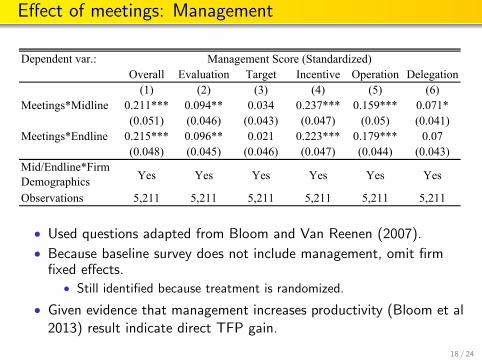
Effect of meetings: Management

Dependent var.:Overall Evaluation Target Incentive Operation Delegation

(1) (2) (3) (4) (5) (6)Meetings*Midline 0.211*** 0.094** 0.034 0.237*** 0.159*** 0.071*

(0.051) (0.046) (0.043) (0.047) (0.05) (0.041)Meetings*Endline 0.215*** 0.096** 0.021 0.223*** 0.179*** 0.07

(0.048) (0.045) (0.046) (0.047) (0.044) (0.043)Mid/Endline*Firm Demographics Yes Yes Yes Yes Yes Yes

Observations 5,211 5,211 5,211 5,211 5,211 5,211

Table 5. Effect of Meetings on Firm Management

Management Score (Standardized)

• Used questions adapted from Bloom and Van Reenen (2007).

• Because baseline survey does not include management, omit firmfixed effects.

• Still identified because treatment is randomized.

• Given evidence that management increases productivity (Bloom et al2013) result indicate direct TFP gain.

18 / 24

Group composition and peer effects

Dependent var.: log Sales Profit (10,000 RMB)

log Num of Employees

log Productivity

log Num of Clients

log Num of Suppliers

Management

(1) (2) (3) (4) (5) (6) (7)Midline*log Peer Size 0.118*** 36.66*** 0.037 0.117*** 0.044* -0.03 0.21***

(0.0322) (11.47) (0.023) (0.036) (0.024) (0.03) (0.035)Endline*log Peer Size 0.166*** 52.25*** 0.015 0.166*** 0.108*** -0.035 0.111***

(0.0464) (17.27) (0.038) (0.043) (0.034) (0.037) (0.035)Firm FE Yes Yes Yes Yes Yes Yes NoMid/Endline*Firm Demographics Yes Yes Yes Yes Yes Yes Yes

Observations 4,183 4,076 4,183 4,029 4,173 4,170 2,774

Table 6. Effect of Peer Firm Size on Performance

• Internal consistency test: if meetings matter, composition shouldalso affect performance.

• Conditional on being in the same region, size category and industrycategory, firms were randomly allocated into groups.

• Control for Midline and Endline interacted with these demographicsand all their interactions.

• For management we do not include firm fixed effects.

19 / 24

Discussion

• Concerns with identification and interpretation.1 Experimenter demand effects.

• Book sales agree with self-reported sales.• Peer effects only compare within treatment group.

2 Side-effects of meetings: better access to government officials.• Peer effects only compare within treatment group.

3 Collusion versus improved performance.• Positive effects on innovation, management score, employment,

number of partners suggest genuine performance gains.

• Broad channels suggested by results so far:

1 Learning from peers (possible channel for management/productivity).2 Improved access to partners.3 Improved access to finance.

20 / 24

Mechanism 1: learning

Dependent var.:(1) (2) (3) (4) (5)

Sample:Info 0.300*** 0.370***

(0.0208) (0.0227)No Info * Meetings 0.202***

(0.0247)Info * Meetings 0.0721**

(0.0323)Having Informed Group Members 0.315*** 0.402***

(0.0340) (0.0470)Competition -0.155*** -0.0715**

(0.0497) (0.0344)Having Informed Group Members -0.173*** *Competition (0.0605)Firm Demographics No No Yes Yes YesObservations 2,646 2,646 846 846 846

Applied for the Firm Funding Product

All Firms Uninformed Firms in Meetings

• Distributed information to randomly chosen managers about:• A funding opportunity for the firm, likely perceived to be rival.• A savings opportunity for the manager, likely less rival.

• Created variation in share of informed managers. 21 / 24

Learning about a savings product

Dependent var.:(1) (2) (3) (4) (5)

Sample:Info 0.398*** 0.542***

(0.0182) (0.0232)No Info * Meetings 0.276***

(0.0276)Info * Meetings 0.00697

(0.0217)Having Informed Group Members 0.328*** 0.311***

(0.0310) (0.0462)Competition -0.00781 -0.0224

(0.0416) (0.0380)Having Informed Group Members 0.0456 *Competition (0.0615)Firm Demographics No No Yes Yes YesObservations 2,646 2,646 835 835 835

Applied for the Private Saving Product

All Firms Uninformed Firms in Meetings

• For less rival private savings product, competition was notsignificantly related to diffusion.

22 / 24

Mechanism 2: partnering

Panel A DifferenceIn Regular Group In Cross Group

Mean 2.18 0.06 2.13***Standard Deviation (0.083) (0.62) (0.079)

Panel B DifferenceIn Regular Group In Cross Group

Mean 1.44 0.29 1.15***Standard Deviation (1.49) (1.52) (0.07)

Panel C DifIn Regular Group In Cross Group

Mean 3.52 0.94 2.58***Standard Deviation (0.13) (0.12) (0.12)

Number of Referrers

Number of Direct Partners

Choice in Trust game

• We also conducted one-time cross-group meetings.• Direct evidence on partnering: more partners in regular than in cross

group.• Consistent with repeated interactions and social capital helping

create relationships.23 / 24

Mechanism 3: access to finance

Dependent var.:Access to

Credit OLS Discussion of

CreditAccess to Credit IV

(1) (2) (3)Post 0.1036* -0.0571

(0.0603) (0.0941)Discussion of Credit*Post 0.0732*** 0.2517*

(0.0283) (0.1417)Share of peers with credit demand at baseline 0.1891***

(0.0673)Share of peers with a loan at baseline 0.3944***

(0.0805)Observations 4,183 1,409 4,183Firm FE Yes No YesFirm Demographics No Yes NoR-squared 0.062 0.1348 0.012Robust standard errors clustered by meeting group in parentheses.*** p<0.01, ** p<0.05, * p<0.1

access to credit =1 if have bank or informal loan

Table 13. Effect of Discussing Credit on Credit

• Measure in logs whether group discussed finance at least twice.• Instrument with share of peers that have credit demand.• When more peers have credit demand, finance discussed more often,

and firm is more likely to borrow.24 / 24